Resolution Study for three-dimensional Supernova Simulations with the Prometheus-Vertex Code

Abstract

We present a carefully designed, systematic study of the angular resolution dependence of simulations with the Prometheus-Vertex neutrino-hydrodynamics code. Employing a simplified neutrino heating-cooling scheme in the Prometheus hydrodynamics module allows us to sample the angular resolution between 4^∘ and 0.5^∘. With a newly-implemented static mesh refinement (SMR) technique on the Yin-Yang grid, the angular coordinates can be refined in concentric shells, compensating for the diverging structure of the spherical grid. In contrast to previous studies with Prometheus and other codes, we find that higher angular resolution and therefore lower numerical viscosity provides more favorable explosion conditions and faster shock expansion. We discuss the possible reasons for the discrepant results. The overall dynamics seem to converge at a resolution of about $1^{\circ}$. Applying the SMR setup to marginally exploding progenitors is disadvantageous for the shock expansion, however, because kinetic energy of downflows is dissipated to internal energy at resolution interfaces, leading to a loss of turbulent pressure support and a steeper temperature gradient. We also present a way to estimate the numerical viscosity on grounds of the measured turbulent kinetic-energy spectrum, leading to smaller values that are better compatible with the flow behavior witnessed in our simulations than results following calculations in previous literature. Interestingly, the numerical Reynolds numbers in the turbulent, neutrino-heated postshock layer (some 10 to several 100) are in the ballpark of expected neutrino-drag effects on the relevant length scales. We provide a formal derivation and quantitative assessment of the neutrino drag terms in an appendix.

1 Introduction

The explosion mechanism of core-collapse supernovae, whether energized by neutrino heating or mediated by magnetic fields, is a generically multi-dimensional phenomenon, in which hydrodynamic instabilities play a crucial role. They do not only foster the explosion but also create initial asymmetries that determine the emerging geometry of the stellar blast. Three-dimensional (3D) hydrodynamical simulations are therefore indispensable, and because of the increasing power of modern massively parallel supercomputers they have recently become possible in combination with elaborate energy-dependent three-flavor neutrino transport (for a review of recent developments, see Janka et al., 2016). Correspondingly, the pool of 3D stellar core-collapse and explosion simulations with substantially different treatments of neutrino transport and physics is growing rapidly (e.g., Takiwaki et al., 2012, 2014; Melson et al., 2015a, b; Lentz et al., 2015; Roberts et al., 2016; Müller et al., 2017, 2019; Summa et al., 2018; Ott et al., 2018; O’Connor & Couch, 2018; Kuroda et al., 2018; Glas et al., 2019; Vartanyan et al., 2019; Burrows et al., 2019).

These simulations were conducted with different grid geometries (Cartesian grids with static or adaptive mesh refinement, cubed-sphere multi-block grids, polar coordinates, Yin-Yang spherical grids, spherical grids with polar mesh coarsening) and with largely different numerical resolutions. While a number of resolution studies have already been performed by varying, within rather close limits, the mesh spacing for fixed grid geometries (e.g., Hanke et al., 2012; Couch & O’Connor, 2014; Abdikamalov et al., 2015; Roberts et al., 2016; Radice et al., 2016; Summa et al., 2018; O’Connor & Couch, 2018), possible numerical artifacts of the grid geometries themselves are still completely unexplored in 3D supernova calculations.

The recognition that nonradial mass motions and buoyant bubble rise in the neutrino-heating layer have an impact on the shock evolution that can be coined in terms of turbulent (pressure, energy transport, dissipation) effects (e.g., Murphy et al., 2013; Couch & Ott, 2015; Müller & Janka, 2015; Radice et al., 2016; Mabanta & Murphy, 2018), has led to increasing interest in the resolution dependence of the turbulent kinetic-energy cascade for the postshock flow in supernova models (Abdikamalov et al., 2015; Radice et al., 2015, 2016, 2018). Low resolution can be imagined to cause enhanced numerical viscosity, which might quench the growth of convective buoyancy, damp nonradial flows, and lead to viscous dissipation of kinetic energy and associated numerical heating. In the regime where growth of the standing accretion-shock instability (SASI; Blondin et al., 2003; Blondin & Mezzacappa, 2007) rather than neutrino-driven convection is favored (see Foglizzo et al., 2006, 2007), low radial resolution can suppress the growth of SASI (Sato et al., 2009), whereas reduced angular resolution can strengthen SASI activity because of weaker or absent parasitic Kelvin-Helmholtz and Rayleigh-Taylor instabilities, which would redistribute kinetic energy from the large SASI scales to vortex flows on smaller scales (Guilet et al., 2010). These expectations from theoretical and toy-model considerations are in line with full-fledged supernova simulations (Summa et al., 2018).

Moreover, Radice et al. (2015, 2016) diagnosed the so-called bottleneck effect, where the lack of resolution prevents kinetic-energy cascading to small scales and leads to an accumulation of kinetic energy on scales larger than the dissipation scale. For this reason the turbulent energy spectra exhibit enhanced power on these scales and display a more shallow decline than expected in the inertial range from Kolmogorov’s classical theory. The authors argued that this circumstance might explain why in previous studies by Hanke et al. (2012) with the Prometheus supernova code—and confirmed by others (e.g., Couch & O’Connor, 2014; Abdikamalov et al., 2015; Roberts et al., 2016) with different numerical methods—lower resolution had fostered earlier and stronger explosions in 3D simulations.

In the present work we report results of a recent, carefully designed resolution study with the Prometheus-Vertex code, sampling angular cell sizes between $4^{\circ}$ and $0.5^{\circ}$ in full-$4\pi$ simulations of the post-bounce evolution of collapsing and exploding 9 $M_{\odot}$ and 20 $M_{\odot}$ stars. We employ full-fledged ray-by-ray neutrino transport with state-of-the-art neutrino interactions, or, alternatively for systematic resolution variations, a simple neutrino-heating and cooling scheme in the form of an improved version of the treatment by Hanke et al. (2012).

Our results reveal exactly the opposite resolution dependence compared to previous investigations, namely that better resolution leads to improved explosion conditions and faster shock expansion in 3D. Our results challenge the interpretation of the previous findings as discussed by Couch & O’Connor (2014), Abdikamalov et al. (2015), and Radice et al. (2016). We understand the behavior witnessed in our models as a consequence of the fact that lower numerical viscosity in the case of higher resolution permits an enhanced level of nonradial (turbulent) kinetic energy in the postshock layer. The conflict with the simulations by Hanke et al. (2012) can be resolved when one takes into account the numerical artifacts associated with the polar axis of the spherical coordinate grid used in those older simulations. In contrast, the supernova models generated in the present work employed the axis-free Yin-Yang grid (Kageyama & Sato, 2004; Wongwathanarat et al., 2010). The Yin-Yang grid reduces numerical artifacts to a much lower level by avoiding axis features as well as effects caused by the nonuniform sizes of azimuthal grid cells at different latitudes, which implies finer spatial resolution near the poles. The question arises why Cartesian 3D simulations reproduced the polar-axis-triggered resolution trend seen by Hanke et al. (2012). We speculate, however without having any foundation by own results, that numerical noise induced on radial flows by Cartesian grids could play an important role. A decreased level of such perturbations when the resolution was improved, might have delayed the onset of explosions in the better-resolved simulations performed by Couch & O’Connor (2014), Abdikamalov et al. (2015), Roberts et al. (2016) and O’Connor & Couch (2018).

We also discuss results obtained with a static mesh refinement (SMR) technique that we implemented on the Yin-Yang grid of the Prometheus-Vertex code. Despite offering enhanced angular resolution in the turbulent postshock layer, it turned out to have an unfavorable influence on the onset and development of explosions in cases that were marginally hitting success. We could trace this back to a conversion of kinetic energy to thermal energy (with the sum of both conserved) in mass flows crossing the borders from grid domains with better to those with coarser resolution. This might suggest additional artifacts that could be associated with the use of static or adaptive mesh refinement procedures used in most applications of Cartesian grids.

Our resolution study indicates that convergence of the shock evolution might be approached at an angular resolution of about $1^{\circ}$. An even more detailed realization of the turbulent power spectrum than it is possible with this resolution seems to have a minor impact on the overall post-bounce dynamics in the supernova core, as most of the energy is contained on the largest scales. Increasing the resolution beyond this point to accurately follow the turbulent energy cascade needs to take into account the effects of neutrino drag, because even for our lowest-resolved simulations neutrino-drag effects begin to compete with the consequences of numerical viscosity on all scales that yield relevant contributions to the turbulent kinetic energy. We provide detailed estimates of the numerical viscosity and Reynolds number (deduced from the numerically realized turbulent kinetic energy spectrum) as well as, in an extended appendix, a detailed discussion of the neutrino-drag effects in the gain layer behind the supernova shock.

Our paper is structured as follows. In Section 2, we briefly describe the numerical setup of our models. The results of our 3D simulations with Vertex neutrino transport are discussed in Section 3. Our systematic resolution study employing the simple neutrino-heating and cooling scheme is presented in Section 4. In Section 5, we focus on a discussion of turbulence in our models and present our method of deducing the numerical viscosity. An assessment of our results in a broader context is the contents of Sect. 6, followed by our summary and conclusions in Section 7. Appendix A provides a concise description of our SMR technique, and Appendix B contains a detailed derivation of the neutrino-drag terms with order-of-magnitude estimates for supernova conditions as well as an evaluation based on simulation results with full neutrino transport.

2 Numerical setup

We performed one-dimensional (1D), two-dimensional (2D), and three-dimensional (3D) core-collapse supernova simulations using two neutrino treatments. The first set of models was computed with the Prometheus-Vertex code (Rampp & Janka, 2002; Buras et al., 2006), whereas the second model set was simulated using only the hydrodynamics module Prometheus (Fryxell et al., 1989, 1991; Müller et al., 1991) with a simplified heating-cooling (HTCL) scheme, based on an improved version of the treatment applied by Hanke et al. (2012). Prometheus is an implementation of the Piecewise Parabolic Method (PPM; Colella & Woodward, 1984)—a Godunov-type scheme being second-order accurate in space and second-order in time.

In all simulations presented in this work, the collapse phase was computed in spherical symmetry with the Prometheus-Vertex code using multi-group neutrino transport and state-of-the-art neutrino interactions. Gravity was treated in spherical symmetry with general-relativistic corrections (Marek et al., 2006, Case A). The high-density equation of state by Lattimer & Swesty (1991) with a nuclear incompressibility of $K=220\,\mathrm{MeV}$ was employed.

For the present study, we selected various angular grid resolutions, while the radial grid was kept unchanged for a given progenitor for comparison. In addition to 3D simulations with uniform angular resolution in the whole computational domain, we also made use of a newly-implemented static mesh refinement (SMR) procedure. It allows us to change the angular resolution in radial layers of the spherical grid. A detailed description of this method can be found in Appendix A.

Table 1: Overview of the simulations discussed in this work.

Model	Progenitor mass	Neutrino scheme	Dimensionality	Angular resolution	1D core
s9.0	$9\,M_{\odot}$	Full transport	3D (Yin-Yang grid)	$3.5^{\circ}$	1.6 km
			3D (Yin-Yang grid)	SMR (up to $0.5^{\circ}$)	1.6 km
s20	$20\,M_{\odot}$	Full transport	3D (Spherical polar grid)	$2^{\circ}$	10 km
			3D (Yin-Yang grid)	SMR (up to $0.5^{\circ}$)	1.6 km
HTCL_4.0	$20\,M_{\odot}$	HTCL with $L_{\nu,52}=4$	1D	-	-
			2D	$0.5^{\circ}$ to $4^{\circ}$	$10^{12}\,\mathrm{g\,cm^{-3}}$
			3D (Yin-Yang grid)	$0.5^{\circ}$ to $4^{\circ}$	$10^{12}\,\mathrm{g\,cm^{-3}}$
			3D (Yin-Yang grid)	SMR (up to $0.5^{\circ}$)	$10^{12}\,\mathrm{g\,cm^{-3}}$
HTCL_3.96	$20\,M_{\odot}$	HTCL with $L_{\nu,52}=3.96$	1D	-	-
			2D	$0.5^{\circ}$ to $4^{\circ}$	$10^{12}\,\mathrm{g\,cm^{-3}}$
			3D (Yin-Yang grid)	$0.5^{\circ}$ to $4^{\circ}$	$10^{12}\,\mathrm{g\,cm^{-3}}$
			3D (Yin-Yang grid)	SMR (up to $0.5^{\circ}$)	$10^{12}\,\mathrm{g\,cm^{-3}}$

In Table 1, we present an overview of all simulations discussed in this work.

2.1 Models with neutrino transport

The first model set was computed using the Prometheus-Vertex code with three-flavor, energy-dependent, ray-by-ray-plus neutrino transport including state-of-the art neutrino interactions. We simulated the post-bounce evolution of a $9\,M_{\odot}$ star (s9.0; Woosley & Heger, 2015) and a $20\,M_{\odot}$ progenitor (s20; Woosley & Heger, 2007). When mapping from 1D to 3D at 10 ms after bounce, random cell-to-cell density perturbations of 0.1 % were imposed to break spherical symmetry.

Besides a setup with uniform angular resolution of $3.5^{\circ}$ and $2^{\circ}$, respectively, we also used an SMR setup with a first refinement step from $2^{\circ}$ to $1^{\circ}$ at the bottom of the gain layer. To maintain a high resolution in the gain layer over time, this SMR interface follows the contraction of the gain radius. A second refinement region with a resolution of $0.5^{\circ}$ was added at 70 ms after bounce exterior to a fixed radius of 160 km. Thus, the resolution was improved twice by a factor of two.

The s20 simulation with a constant $2^{\circ}$ angular resolution was published before in Melson et al. (2015a) and computed on a spherical polar grid with a core of 10 km treated spherically symmetrically. All other runs in this model set were evolved on the Yin-Yang grid (Kageyama & Sato, 2004; Wongwathanarat et al., 2010) with a smaller 1D core of 1.6 km radius. The radial grid was gradually refined from 400 zones to more than 600 to account for the steepening of the density gradient at the proton-neutron star surface.

2.2 Models with simplified heating-cooling scheme

For the HTCL model set, the $20\,M_{\odot}$ progenitor from Woosley & Heger (2007) was selected. The multi-dimensional simulations were started from a 1D collapse run and mapped to 2D/3D at 15 ms after bounce. At this stage, random cell-to-cell density perturbations were imposed with an amplitude of 0.1 %.

The radial grid was set to 400 zones in all models and kept constant in time. Since the proto-neutron star remains larger in the HTCL simulations and no transport is applied, this radial grid yields sufficient resolution, compatible with what is used in Prometheus-Vertex for neutron stars of similar radius. Note that the simplified HTCL scheme is not subject to the same resolution constraints as detailed neutrino transport. Moreover, the purpose of our simulations with the HTCL treatment is not a most accurate description of the neutron star and its near-surface layers, but instead the goal is a study of turbulence and resolution effects in the postshock domain.

The central region enclosed by the density contour of $10^{12}\,\mathrm{g\,cm^{-3}}$ was treated in spherical symmetry, corresponding to a radius of 42–46 km. This radius is considerably larger than in the simulations with full-fledged neutrino transport, because the simplified HTCL scheme weakens the contraction of the proto-neutron star. We will comment on the consequences of this fact at several places in the discussion of our results.

All 3D simulations in this model set were computed on the Yin-Yang grid. Besides the runs with a constant angular resolution in the entire computational domain, we used the SMR grid with a resolution of $2^{\circ}$ up to a radius of 123 km and $1^{\circ}$ outside. At 150 ms after bounce, an additional layer of $0.5^{\circ}$ angular resolution was added outside a radius of 162 km, thus improving the resolution a second time by a factor of two. Note that the imposed initial perturbation patterns were identical in the SMR case and the $2^{\circ}$ run.

The HTCL scheme was used already in a 3D study by Hanke et al. (2012). However, our implementation of this scheme and other aspects of our presented study differ in some details. First, Hanke et al. (2012) used a spherical polar grid instead of the Yin-Yang grid. Second, they employed a Newtonian gravitational potential without general-relativistic corrections. Third, the high-density equation of state of Lattimer & Swesty (1991) with $K=180\,\mathrm{MeV}$ was used in their work. Also our formulation of the heating and cooling terms was modified compared to theirs. Our heating and cooling terms read, respectively,

$$\begin{split}\dot{q}_{\mathrm{heat}}=&1.544\times 10^{20}\left(\frac{L_{\nu}}{10^{52}\,\mathrm{erg\,s^{-1}}}\right)\left(\frac{100\,\mathrm{km}}{r}\right)^{2}\\ &\times\left(\frac{T_{\nu}}{4\,\mathrm{MeV}}\right)^{2}\left(Y_{n}+Y_{p}\right)e^{-\tau_{\mathrm{eff}}/2}\,\mathrm{erg\,g^{-1}\,s^{-1}},\end{split}$$ (1)

and

$$\begin{split}\dot{q}_{\mathrm{cool}}=&1.399\times 10^{20}\left(\frac{T}{2\,\mathrm{MeV}}\right)^{6}\left(Y_{n}+Y_{p}\right)\\ &\times e^{-\tau_{\mathrm{eff}}/2}\,\mathrm{erg\,g^{-1}\,s^{-1}},\end{split}$$ (2)

where $r$ is the radius and $T$ is the temperature. $Y_{n}$ and $Y_{p}$ are the neutron and proton number fractions, respectively. $L_{\nu,52}\equiv L_{\nu}/(10^{52}\,\mathrm{erg\,s^{-1}})$ is a free parameter with two different values of 3.96 and 4.0 in this work. The neutrino temperature $T_{\nu}$ is set to 4 MeV. The exponential term $\tau_{\mathrm{eff}}$ is given by

$$\tau_{\mathrm{eff}}(r)=\int_{r}^{\infty}\mathrm{d}r^{\prime}\,\kappa_{\mathrm{eff}}(r^{\prime}),$$ (3)

with

$$\kappa_{\mathrm{eff}}=7.5\times 10^{-8}\left(\frac{\rho}{10^{10}\,\mathrm{g\,cm^{-3}}}\right)\left(\frac{T_{\nu}}{4\,\mathrm{MeV}}\right)^{2}\,\mathrm{cm^{-1}},$$ (4)

where $\rho$ is the mass density.

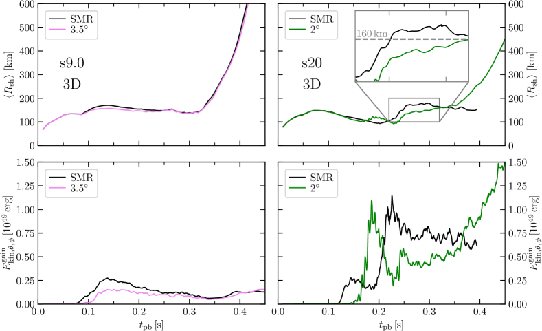
Figure 1: Post-bounce evolution of the 3D models computed with full neutrino transport, s9.0 (left) and s20 (right), for different angular grid resolutions. Top: Angle-averaged shock radius, $\left<R_{\mathrm{sh}}\right>$. The gray dashed line in the zoom inset of the right panel indicates the location of the outer SMR refinement interface. Bottom: Nonradial kinetic energy in the gain layer, $E^{\mathrm{gain}}_{\mathrm{kin},\theta,\phi}$.

Because of the combination of all differences, the parameter $L_{\nu,52}$ in our scheme is about a factor of four higher than in the work by Hanke et al. (2012) in order to trigger shock revival.

3 Models with neutrino transport

In Fig. 1, we show the angle-averaged shock radii as functions of post-bounce time for the two progenitors evolved with full neutrino transport. In the s9.0 case, the temporal evolution of the shock remains nearly unaffected by a change of the angular resolution from a uniform $3.5^{\circ}$ grid to the SMR setup. Only between $\sim$100 ms and $\sim$250 ms after bounce, the shock in the SMR case has a slightly larger radius. However, the time of shock revival and also the shock expansion velocity are nearly identical in both setups. The reason for this is the robustness of the explosion in the s9.0 model. It is well beyond the critical explosion threshold, because the mass-accretion rate in this low-mass progenitor decreases rapidly at the silicon/silicon+oxygen interface leading to a significant drop in the ram pressure at the shock.

In the s20 model, the simulation with a uniform grid behaves entirely differently from the SMR case. The former explodes, while the latter does not experience shock revival until we stopped the simulation at 400 ms after core bounce. Between 200 and 300 ms, the SMR model seems to have more favorable explosion conditions because of a larger shock radius. Also the nonradial kinetic energy in the gain layer, defined by

$$E_{\mathrm{kin},\theta,\phi}^{\mathrm{gain}}\equiv\int_{R_{\mathrm{gain}}<r<R_{\mathrm{sh}}(\theta,\phi)}\mathrm{d}V\,\frac{1}{2}\rho\left(v_{\theta}^{2}+v_{\phi}^{2}\right)$$ (5)

and shown in the lower row of Fig. 1, is much higher during this time interval, because of a strong SASI spiral mode being present in the SMR model. $R_{\mathrm{gain}}$ is the angle-averaged gain radius. At about 350 ms, however, this picture changes and the simulation with a fixed resolution of $2^{\circ}$ explodes, whereas the kinetic energy in the gain layer decreases continuously in the SMR case.

In contrast, the s9.0 simulations do not differ much in their lateral kinetic energies in the gain layer at the time when the explosions set it. Although the SMR model develops higher values transiently, convective overturn becomes similar in both simulations after 250 ms.

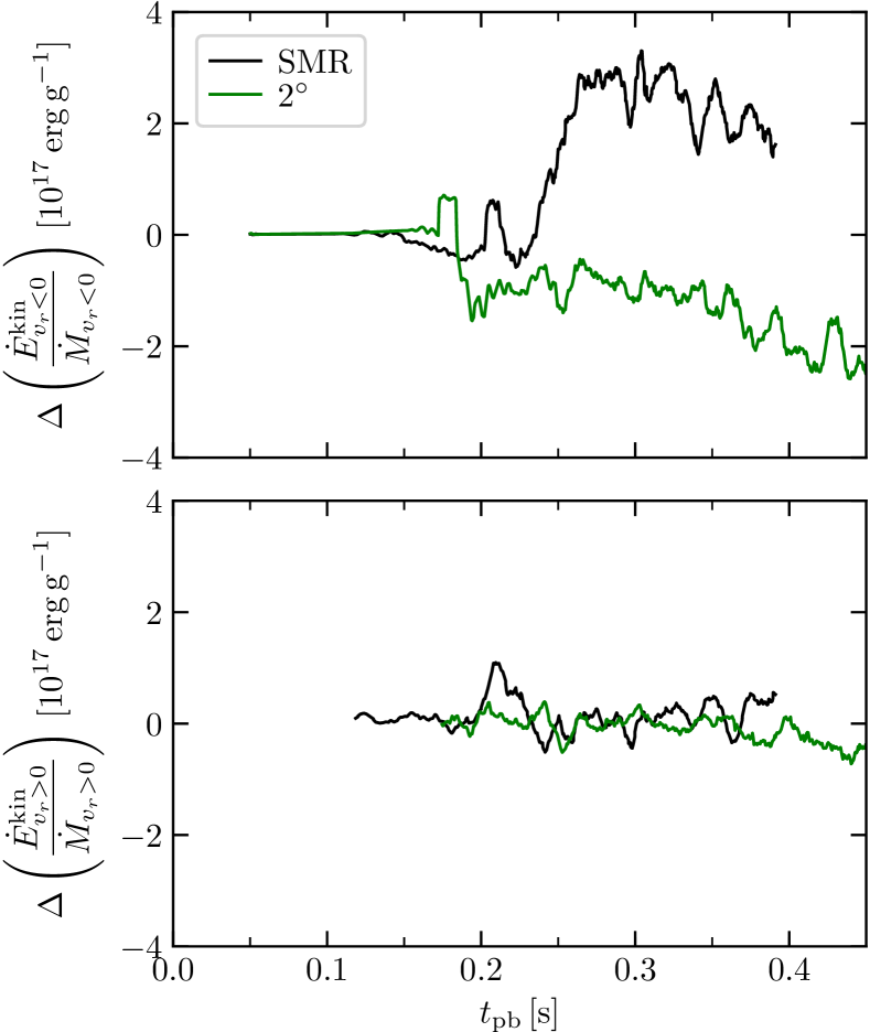
Figure 2: Difference of the radial kinetic energy flux divided by the radial mass flux as a function of post-bounce time, $t_{\mathrm{pb}}$, for the s20 models computed with full neutrino transport. The values at a radius 1 km below the inner SMR resolution interface are subtracted from the values at a radius 1 km above it, thus probing the flux conservation at this interface, which is moved inward from initially 105 km to 64 km during the simulation. At this radius, the angular resolution increases outward from $2^{\circ}$ to $1^{\circ}$ in the SMR run. Note that both the minuend and the subtrahend are always positive. The plotted values are time-averaged with a window of 10 ms. We differentiate between inflows (top) and outflows (bottom).

In order to understand why the SMR setup with its angular resolution of $1^{\circ}$ in the gain layer and even $0.5^{\circ}$ above 160 km prevents shock revival in the s20 model despite the higher nonradial kinetic energy over a period of 200 ms, we investigate the dissipation of kinetic energy at the interfaces between resolution layers. We speculate that this effect might be crucial especially in regions close to the gain radius, where neutrino heating is strongest and its interplay with the turbulent flow dynamics most pronounced.

In Fig. 2, we thus show differences of the radial fluxes of kinetic energy across the inner SMR interface (which is located at the bottom of the gain layer) for inflowing and outflowing material for the s20 models. The kinetic energy fluxes are computed according to

$$\dot{E}^{\mathrm{kin}}_{v_{r}<0} \equiv r^{2}\int\mathrm{d}\Omega\,\Theta(-v_{r})\,\frac{1}{2}\rho\left(v_{r}^{2}+v_{\theta}^{2}+v_{\phi}^{2}\right)v_{r},$$ (6)

$$\dot{E}^{\mathrm{kin}}_{v_{r}>0} \equiv r^{2}\int\mathrm{d}\Omega\,\Theta(v_{r})\,\frac{1}{2}\rho\left(v_{r}^{2}+v_{\theta}^{2}+v_{\phi}^{2}\right)v_{r},$$ (7)

and the mass fluxes are given by

$$\dot{M}_{v_{r}<0} \equiv r^{2}\int\mathrm{d}\Omega\,\Theta(-v_{r})\,\rho v_{r},$$ (8)

$$\dot{M}_{v_{r}>0} \equiv r^{2}\int\mathrm{d}\Omega\,\Theta(v_{r})\,\rho v_{r},$$ (9)

where $\Theta(x)$ is the Heaviside step function. Both quantities are evaluated as integrals over inflows ($v_{r}<0$) and outflows ($v_{r}>0$) separately. The differences are calculated by subtracting the specific kinetic energy fluxes at a radius 1 km below the inner SMR resolution interface, $r_{1}$, from their values at a radius 1 km above it, $r_{2}$. For outflows, for example, we get

$$\Delta\left(\frac{\dot{E}^{\mathrm{kin}}_{v_{r}>0}}{\dot{M}_{v_{r}>0}}\right)=\frac{\dot{E}^{\mathrm{kin}}_{v_{r}>0}(r_{2})}{\dot{M}_{v_{r}>0}(r_{2})}-\frac{\dot{E}^{\mathrm{kin}}_{v_{r}>0}(r_{1})}{\dot{M}_{v_{r}>0}(r_{1})}\,.$$ (10)

This allows us to investigate the flux conservation at this resolution interface, which is moved inward during the simulation from initially 105 km down to 64 km, roughly following the contraction of the gain radius. The individual terms in Eq. (10) are always positive at both radii so that a positive difference represents a higher flux at the outer radius for both flow directions.

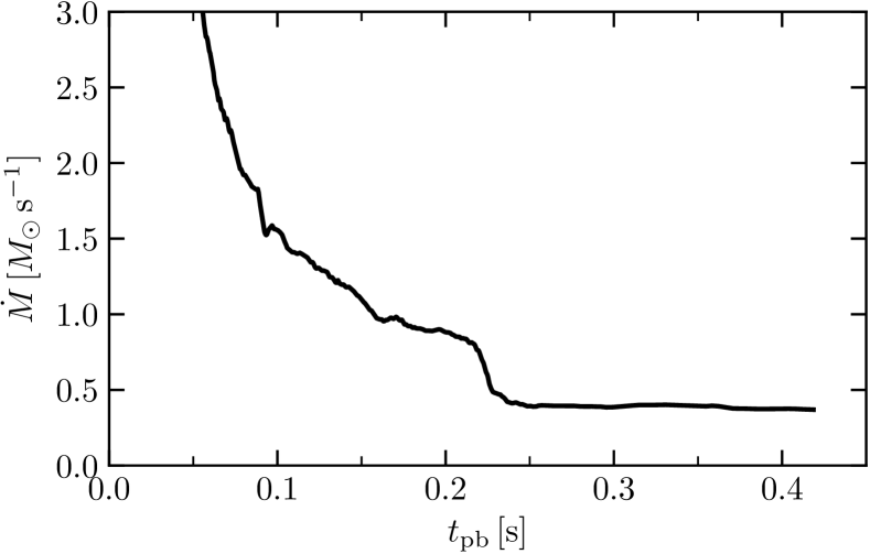
Figure 3: Mass-accretion rate, $\dot{M}$, of the s20 progenitor as a function of post-bounce time, $t_{\mathrm{pb}}$, measured at a radius of $400\,\mathrm{km}$.

On the SMR grid, matter flowing inwards is passing from the region with an angular resolution of $1^{\circ}$ to the layer with a grid spacing of $2^{\circ}$ at the inner SMR interface. We wonder whether dissipation of kinetic energy occurs as a consequence of the averaging over neighboring grid cells when the grid resolution decreases (see Appendix A). Especially, investigating this effect at the arrival time of the silicon/silicon+oxygen interface is important, because this is the crucial phase for shock revival. At that time, the preshock mass-accretion rate defined (at 400 km) by

$$\dot{M}\equiv-r^{2}\int\mathrm{d}\Omega\,\rho v_{r}$$ (11)

and thus also the ram pressure at the shock drops significantly, which happens at about 230 ms in the s20 progenitor (cf. Fig. 3). Until about that time, the energy differences are very similar in both models (Fig. 2, upper panel). But shortly after that, at about 240 ms, the difference in the specific kinetic energy fluxes as displayed in the top panel of Fig. 2 starts to rise steeply in the SMR simulation. In contrast, it remains even below zero in the model with uniform $2^{\circ}$ resolution, meaning that the absolute value of the inward flux of kinetic energy per unit of mass at the inner radius, $r_{1}$, is higher than at the outer radius, $r_{2}$. The negative value points to a gravitational acceleration of the inward flow. In the SMR model, the steep rise of the energy difference to positive values implies that kinetic energy is dissipated in this case at the resolution interface, which is crossed by matter flow into the coarser-resolved region. Such a dissipation of kinetic energy does not happen in the non-SMR case.

In the bottom panel of Fig. 2, we present the same analysis for outflowing material. Because matter is propagating into the finer-resolved layer in the SMR model, we do not expect kinetic energy to be dissipated into thermal energy. Indeed, the difference of the specific kinetic energy fluxes around the resolution interface remains close to zero for outflowing material, both in the SMR and in the $2^{\circ}$ simulation.

Analogously, dissipation of kinetic energy (of downflows) should also occur at the outer resolution interface of the SMR model, which is located at a fixed radius of 160 km. However, performing the same analysis at this position is complicated by the presence of the deformed shock over an extended period of time. The shock decelerates the radially infalling pre-shock material and thus accounts for most of the reduction in $\dot{E}^{\mathrm{kin}}_{v_{r}<0}/\dot{M}_{v_{r}<0}$ during this phase, covering the dissipation effect of the grid geometry. Nevertheless, it is suspicious that the average shock radius in the SMR run stagnates just after the shock has passed the interface at 160 km (see zoom inset in Fig. 1). This possibly points towards the dissipation effect associated with the SMR grid.

The question remains, why the dissipation of kinetic energy in the SMR simulation of the s20 model hampers shock revival. Radice et al. (2015) discussed the effects of thermal and turbulent pressure contributions in comparison. With the energy density $e$ and the adiabatic index $\gamma$, the pressure is given by $p=(\gamma-1)e$. For the thermal pressure in the radiation ($e^{\pm}$ pairs and photons) dominated postshock layer, $\gamma\approx 4/3$, whereas for anisotropic turbulence as characteristic for the postshock layer, one has $\gamma=2$. When turbulent kinetic energy is dissipated into thermal energy, the pressure contribution therefore decreases per unit of energy density. For this reason, energy dissipation at SMR resolution interfaces reduces the pressure support behind the shock and possibly prohibits shock revival.

4 Models with simplified heating-cooling scheme

As described in the previous section, the usage of the SMR grid impeded the revival of the shock in the s20 model, although the angular grid resolution was effectively enhanced with this setup. It is therefore crucial to disentangle the influence of a higher uniform grid resolution from the possible detrimental effects of the SMR procedure. We thus performed simulations of the s20 progenitor with a simplified heating-cooling (HTCL) scheme replacing the computing-intense neutrino transport.

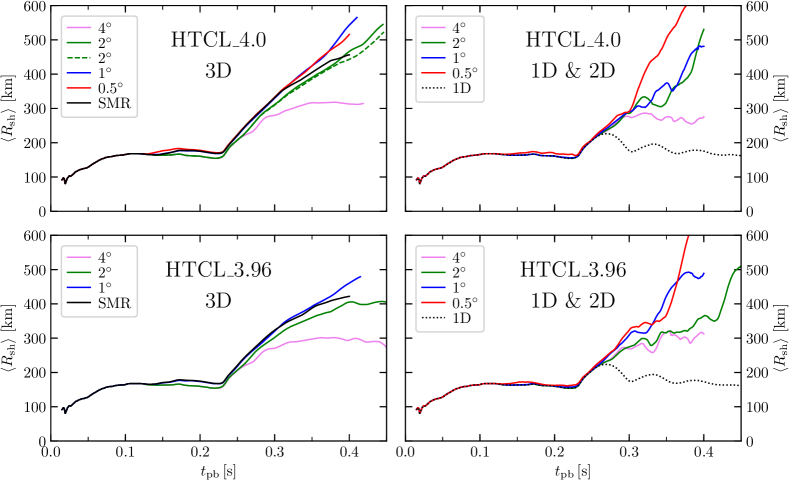
Figure 4: Angle-averaged shock radii of the HTCL models as a function of time with parameter choices $L_{\nu,52}=4$ (top) and $L_{\nu,52}=3.96$ (bottom) in 3D (left), as well as 1D and 2D (right). The 3D model with $L_{\nu,52}=4$ and an angular resolution of $2^{\circ}$ was repeated twice with different initial random perturbation patterns. The model sequences for $L_{\nu,52}=3.96$ exhibit a stronger sensitivity and wider spread in dependence on the angular resolution (in particular for the 2^∘ cases), because the runs are closer to the explosion threshold.

In Fig. 4, we present the angle-averaged shock radii of the entire model set. We selected two different choices for the HTCL parameter $L_{\nu,52}$, 3.96 and 4.0, to control the tendency to get an explosion, namely the strength of neutrino heating to overcome the ram pressure of infalling material.

In almost all simulations of this set, shock revival occurs at the arrival time of the silicon/silicon+oxygen interface (cf. Fig. 3). Only the simulations with a very coarse angular resolution of $4^{\circ}$ and the 1D models do not explode. The latter show the well-known oscillating behavior of the shock radius during the shock stagnation phase. It needs to be pointed out that the simple cooling prescription reduces lepton-number and energy losses by the proto-neutron star and thus weakens its contraction. This, in turn, allows for a larger shock-stagnation radius than in our full-fledged supernova simulations and disfavors SASI activity, in particular in 3D.

The shock expansion velocity at $t_{\mathrm{pb}}\gtrsim 230\,\mathrm{ms}$ is basically a monotonic function of the angular resolution. Higher angular resolution accelerates the propagation of the shock after its revival. This is true both in 2D and 3D, although the angle-averaged shock in 2D propagates in a more oscillatory manner. Note that the presence of the symmetry axis in the 2D models collimates the flow along this axis and enhances the tendency for shock-sloshing motions (see, e.g., Glas et al., 2019). The axial symmetry fosters shock expansion predominantly along the axis, leading to a prolate shape of the shock surface, and because of the importance of shock-sloshing motions it leads to large statistical variations of the angle-averaged shock radius in 2D.

Both simulation sets with $L_{\nu,52}=4$ and $L_{\nu,52}=3.96$ show the same behavior and resolution dependence. Explosions in the latter runs are weaker with a lower shock expansion velocity. In the following discussion, we will focus on the $L_{\nu,52}=4$ model set, because we were able to perform a simulation with a uniform resolution of $0.5^{\circ}$ for this choice of the heating parameter, which was not possible for $L_{\nu,52}=3.96$ due to computing time limitations.

In the 3D models with $1^{\circ}$ and $0.5^{\circ}$ resolution of the $L_{\nu,52}=4$ model set, the shock trajectories behave very similarly until 370 ms. The difference between these two cases is much smaller than relative deviations between any other simulations. We recommend not to overinterpret the difference of the shock trajectories in Fig. 4 between the $1^{\circ}$ and $0.5^{\circ}$ simulations after 370 ms. This difference may be a transient feature connected to the faster rise of a buoyant bubble, which would be a stochastic phenomenon that can change from model to model. To clarify this issue, however, the simulations would have to be continued to later times. For these two cases, we are therefore tempted to conclude that the overall dynamics in 3D converge at about $1^{\circ}$ angular resolution, in particular because most of the kinetic energy is contained in the turbulent flow on the largest scales. However, a final confirmation of convergence would require simulations with increased radial resolution and significantly better angular resolution than $0.5^{\circ}$.

The 3D SMR simulations follow their corresponding highest-resolved uniformly gridded counterparts for a long time. Only after about 300 ms for $L_{\nu,52}=4$ and 350 ms for $L_{\nu,52}=3.96$, the shock velocity decreases. The reason for this behavior is the dissipation of kinetic energy at resolution interfaces, similarly to our findings for the model set with full neutrino transport discussed above. We will analyze this effect in more detail later.

To prove that our analysis does not suffer from stochastical variations in 3D, we repeated the $2^{\circ}$ model in the $L_{\nu,52}=4$ set with a different random cell-to-cell perturbation pattern. Until more than 350 ms, the shock trajectories of the two $2^{\circ}$ simulations remain nearly identical. Only in the very last phase, they start to differ slightly. The resolution trend we see in our models is therefore unlikely to be simply a manifestation of stochastical differences.

Figure 5: Cross-sectional cuts through the 3D HTCL models of the $L_{\nu,52}=4$ model set at 300 ms, 350 ms, and 400 ms after bounce with the color-coded entropy per baryon, $s$.

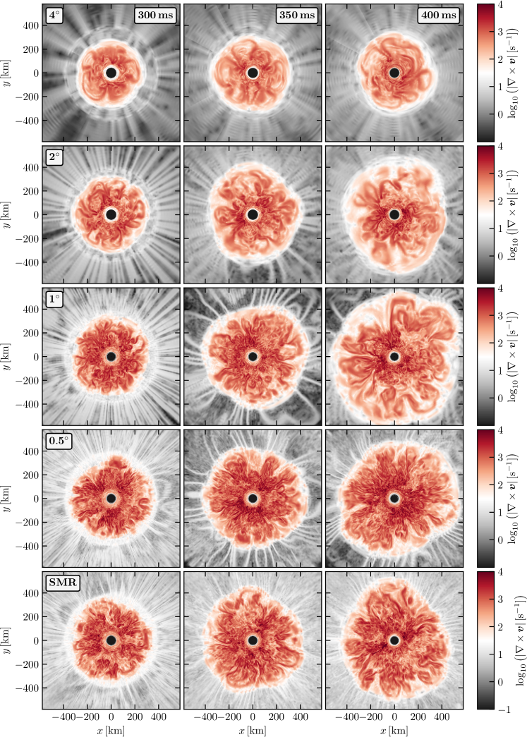
Figure 6: Same as Fig. 5, but with the color-coded vorticity, $|\nabla\times\boldsymbol{v}|$.

In Fig. 5, we show cross-sectional slices through the 3D models with $L_{\nu,52}=4$ at 300 ms, 350 ms, and 400 ms after bounce. All models are dominated by convection and do not develop visible SASI activity, because the shock does not retreat far enough during its stagnation phase to provide suitable conditions for SASI growth.

The color-coded entropy clearly shows that the vortex structures become finer with increasing angular resolution, and downflows develop smaller-structured Kelvin-Helmholtz flow patterns. Especially a comparison of the $0.5^{\circ}$ model with the SMR case does not reveal any noticeable difference. The SMR grid setup seems to provide enough resolution where necessary to allow for the small structures to develop.

In all simulations, we observe clearly separated high-entropy plumes. This is in contrast to the work by Radice et al. (2016), who argued that high-entropy bubbles are embedded in a low-entropy surrounding medium only if the resolution is too low, and that these bubbles should instead form diffuse “clouds”. In our models, we also see that the laminar layer behind the shock surface is similarly structured in all cases and its thickness does not depend on the angular resolution.

The vorticity, $|\nabla\times\boldsymbol{v}|$, shown in Fig. 6 depicts turbulence in the gain layer, with typical values of $\sim 10^{2}-10^{4}\,\mathrm{s^{-1}}$ (red colors). With increasing angular resolution, the volume filled with small-scale turbulent eddies grows. The magnitude of the vorticity, however, does not depend strongly on the resolution. Again, a clear difference between the highest-resolved uniform grid of $0.5^{\circ}$ and the SMR setup cannot be spotted. The radially infalling material ahead of the shock has significantly smaller values of the vorticity compared to the neutrino-heated postshock matter (grey colors). The filament-like structures in this region are a consequence of the random density perturbations of 0.1 % amplitude, which are imposed in the whole computational volume at 15 ms after bounce to break the spherical symmetry of the progenitor model.

At around 150 ms, the higher-resolved 3D models experience a phase of slight shock expansion by about 15 km on average. This is due to convection in the neutrino-heating layer, which gains strength at this time. The nonradial kinetic energy in the gain layer plotted in Fig. 7 shows that postshock convection starts early at $\sim$120 ms in the models with an angular resolution of at least $1^{\circ}$. In lower-resolved cases, this occurs about 100 ms later. The onset of turbulent convection depends on the angular resolution, because low resolution corresponds to a higher numerical viscosity that dampens the rise of buoyant bubbles. In this context, the SMR models behave similarly to the cases with $1^{\circ}$ angular resolution, because this is precisely the resolution of the gain layer during the shock stagnation phase in the SMR setup. Note that our simulations do not develop strong SASI activity, because the shock radius does not retreat, disfavoring SASI growth. This is another reason why the lower-resolution models do not develop postshock turbulence before the shock expands after the passage of the silicon/silicon+oxygen interface.

After shock revival, there remains a less pronounced dependence of the lateral kinetic energy on the angular resolution, except for the lowest-resolved models of $4^{\circ}$, which falls clearly behind the others. This relative insensitivity to the resolution is compatible with the fact that most of the kinetic energy is contained by vortex flows on the largest scales.

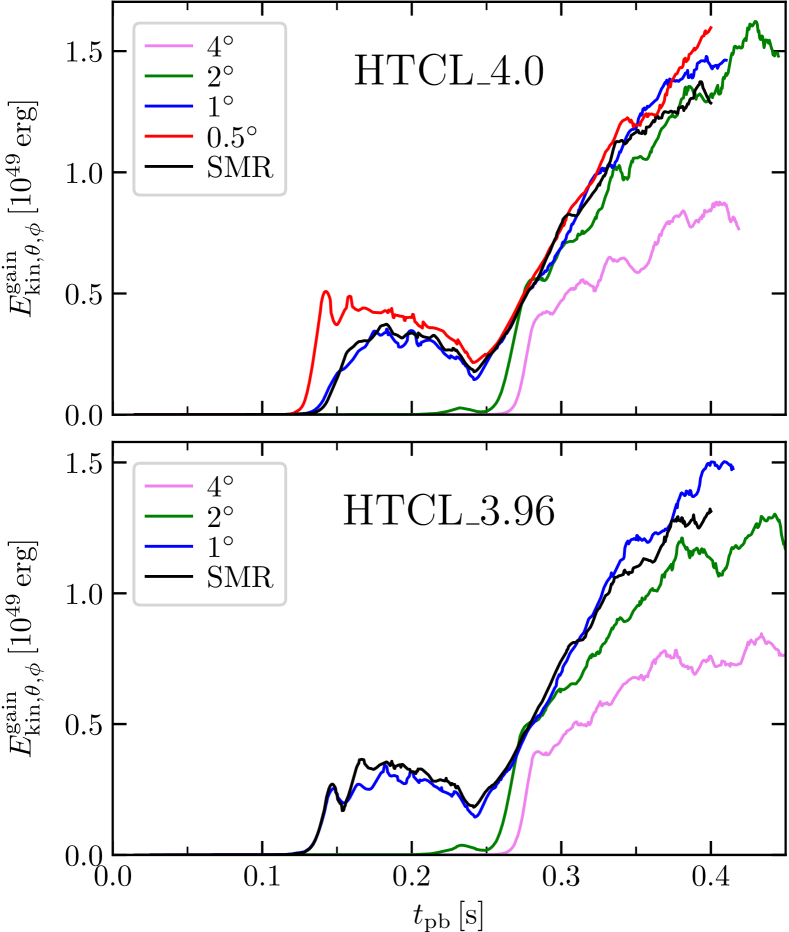
Figure 7: Nonradial kinetic energy in the gain layer as a function of time for the two HTCL model sets with $L_{\nu,52}=4$ (top) and $L_{\nu,52}=3.96$ (bottom).

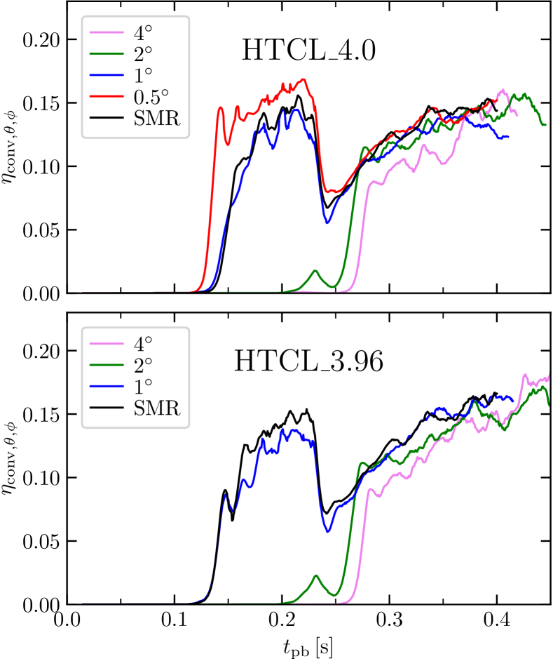
Figure 8: Efficiency factor for the conversion of heating into (nonradial) turbulent kinetic energy as a function of time for the two HTCL model sets with $L_{\nu,52}=4$ (top) and $L_{\nu,52}=3.96$ (bottom).

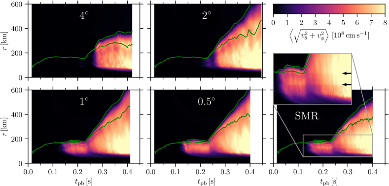
Figure 9: Minimum and maximum shock radii as functions of post-bounce time (green lines) for the HTCL models with $L_{\nu,52}=4$. Color-coded is the density-weighted angle-average of the lateral velocity, $\left<(v_{\theta}^{2}+v_{\phi}^{2})^{0.5}\right>$. The zoom inset attached to the lower right panel shows the positions of the two SMR resolution interfaces (123 and 162 km, black arrows), where nonradial kinetic energy of downflows is converted to thermal energy. The loss of nonradial kinetic energy is visible as faint discontinuities in the color shading at the radial locations of the two black arrows.

As in Müller et al. (2017), we analyze the efficiency for the conversion of neutrino energy deposited in the gain layer into turbulent kinetic energy,

$$\eta_{\mathrm{conv},\theta,\phi}=\frac{E_{\mathrm{kin},\theta,\phi}^{\mathrm{gain}}}{\left[\dot{Q}_{\mathrm{gain}}\left(\left<R_{\mathrm{sh}}\right>-R_{\mathrm{gain}}\right)\right]^{2/3}M_{\mathrm{gain}}^{1/3}},$$ (12)

where $R_{\mathrm{gain}}$ and $M_{\mathrm{gain}}$ are the average gain radius and the gain-layer mass, respectively. The net heating term is given by

$$\dot{Q}_{\mathrm{gain}}\equiv\int_{R_{\mathrm{gain}}<r<R_{\mathrm{sh}}(\theta,\phi)}\mathrm{d}V\,\rho\left(\dot{q}_{\mathrm{heat}}-\dot{q}_{\mathrm{cool}}\right).$$ (13)

The values of $\eta_{\mathrm{conv},\theta,\phi}$ are shown in Fig. 8. Before the arrival of the silicon/silicon+oxygen interface, we see the same dependence on the resolution as in Fig. 7. The models with a resolution of at least $1^{\circ}$ reach an efficiency of about 0.15, while the lower-resolved cases remain convectively less vigorous. After the onset of shock runaway, the conversion efficiency $\eta_{\mathrm{conv},\theta,\phi}$ loses its dependency on the angular resolution if the grid spacing is at least $2^{\circ}$.

The time evolution of the lateral velocities is presented in Fig. 9 as a radius-time diagram. It can be clearly seen that the onset of convection in the gain layer occurs earlier with higher angular resolution, which we have discussed already before. The slight shock expansion at 150 ms after bounce in the models with at least $1^{\circ}$ resolution can be explained by the growing strength of convection at that time. Models that remain convectively quiet do not show this effect. After the revival of the shock, the convective strength, i.e., the magnitude of the lateral velocity is roughly equal in all models presented in Fig. 9. This is in line with the finding that the nonradial kinetic energy does not depend on the angular resolution after the arrival of the silicon/silicon+oxygen interface except for still lower values in the 4^∘ model.

Figure 10: Same as Fig. 2, but for the HTCL model set with $L_{\nu,52}=4$. The difference of the radial specific kinetic energy flux is evaluated around a radius of 123 km, i.e., the specific energy flux at 122 km is subtracted from its value at 124 km. We differentiate between inflows (top) and outflows (bottom).

We have shown above that the SMR setup resembles a uniform grid with a resolution of $0.5^{\circ}$ in the overall fluid structures. Also the temporal evolution of the angle-averaged shock is identical until at least 70 ms after shock revival. Afterwards, however, the expansion velocity of the shock decreases and falls below the case of $1^{\circ}$ resolution. This can again be explained by the dissipation of kinetic energy at the interfaces between layers of different angular resolution (see black arrows in the zoom inset of Fig. 9).

In Fig. 10, the radial specific kinetic energy fluxes are evaluated at two different radii. The value at 122 km is subtracted from the value at 124 km, to investigate the flux conservation at the SMR interface at 123 km. This analysis is performed in the same way as for the model set with full neutrino transport above, but now with $r_{1}=122\,\mathrm{km}$ and $r_{2}=124\,\mathrm{km}$ in Eq. (10). Note that the individual values are always positive for infalling and outflowing fluid elements so that a larger flux at the outer radius results in a positive flux difference.

Again, we see that the outflowing fluxes do not show any evidence for dissipation of kinetic energy. This is assuring especially for the SMR model, where matter flowing outwards is propagating from a coarser grid spacing of $2^{\circ}$ into a finer grid of $1^{\circ}$ resolution. Infalling material, however, behaves differently in this comparison. The flux differences in the models with a uniform grid spacing are rather similar and stay close to zero, whereas in the SMR simulation they are distinctly higher by factors of a few during times of increased nonradial velocities in the gain layer. Kinetic energy is therefore dissipated on the SMR grid with its resolution interface at 123 km as matter flows from 124 km to 122 km. This effect can also be spotted in the bottom right panel of Fig. 9, where the boundaries of the different resolution layers of the SMR grid display as faint horizontal discontinuities in the color shading (see associated zoom inset). The magnitude of the lateral velocity decreases visibly at 162 and 123 km from outside inwards, which would not be the case without kinetic energy dissipation.

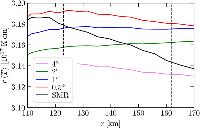
Figure 11: Angle- and time-averaged temperature multiplied with radius for the HTCL simulations with $L_{\nu,52}=4$. The time average was calculated in the interval from 300 to 400 ms. The angular resolution in the SMR model is $2^{\circ}$, $1^{\circ}$, and $0.5^{\circ}$ for $r<123\,\mathrm{km}$, $123\,\mathrm{km}<r<162\,\mathrm{km}$, and $r>162\,\mathrm{km}$, respectively. The boundaries of these regions are indicated by vertical dashed lines.

When kinetic energy is dissipated into thermal energy in the SMR model, the temperature should increase directly below a resolution interface. To analyze this, we show radial profiles of the angle- and time-averaged temperature multiplied with the radius in Fig. 11. This visualization roughly compensates for the $r^{-1}$ scaling of the temperature and allows us to closely analyze temperature gradients.

The temperature profile in the SMR case clearly differs from all other models. It is much steeper and shows an even further increased gradient directly below the inner resolution interface at a radius of 123 km. Between the two resolution layers, i.e. between the two dashed lines in Fig. 11, the SMR profile does not flatten, because the dissipation of kinetic energy does not happen instantaneously as the flow moves inwards. With a radial velocity of about $-3\times 10^{8}\,\mathrm{cm\,s^{-1}}$, a fluid element needs only about 15 ms to propagate through the region of $1^{\circ}$ angular resolution.

We have thus shown that the dissipation of kinetic energy in downflows increases the thermal energy and changes the average temperature profile at the expense of turbulent kinetic energy. For the anisotropic postshock turbulence in the supernova core, kinetic energy and turbulent pressure are coupled by an effective adiabatic index of $\gamma_{\mathrm{turb}}=2$ (Radice et al., 2015). In contrast, thermal energy of the plasma in the postshock layer, where relativistic electron-positron pairs and photons dominate the energy density, provides thermal pressure only with a thermodynamical adiabatic index of $\gamma_{\mathrm{thermal}}\approx 4/3$. This suggests that the conversion of turbulent kinetic energy to thermal energy reduces the ability of the postshock layer to provide outward push to the supernova shock. This explains why at later times, $t_{\mathrm{pb}}\gtrsim 300$ ms, the expansion of the shock in the SMR models begins to slightly lag behind the shock of the $1^{\circ}$ and $0.5^{\circ}$ simulations (see Fig. 4).

5 Resolution dependence of turbulence

In this section, we will investigate how the angular grid resolution influences the turbulent cascade, following the discussion in Melson (2016).

5.1 Turbulent kinetic energy spectra

A fluid transitions from the laminar to the turbulent regime above a certain critical Reynolds number $\mathrm{Re}$. Turbulence is described phenomenologically and understood as a superposition of eddies on various scales (Landau & Lifshitz, 1987; Pope, 2000). In the common picture sharpened by Kolmogorov (1941), kinetic energy is steadily injected at some large scale $L$, which is similar to the size of the largest turbulent eddies. These eddies break up into smaller structures and thus transport energy to successively smaller scales. Eventually, below some small scale $\mathcal{L}$, kinetic energy is dissipated into internal energy by viscous effects.

Kolmogorov (1941) assumed that this turbulent energy cascade only depends on the energy dissipation rate and the viscosity. In the inertial range roughly between $L$ and $\mathcal{L}$, kinetic energy is carried to smaller scales without losses. From a self-similarity ansatz, it follows that the kinetic energy spectrum $E(k)$—with $k$ being the wave number—has a universal shape of $E(k)\propto k^{-5/3}$ in the inertial range. These findings only hold if the fluid structures are locally isotropic, i.e., large-scale anisotropies due to boundary effects can be neglected for sufficiently small scales below $L$ (Pope, 2000). Moreover, ideal conditions require that the fluid is incompressible and the flow is stationary. The last two aspects are certainly not fulfilled in the supernova environment. It is also not clear whether the first assumption is valid during the shock stagnation phase, because the accretion flow through the gain layer might impose a preferred direction not only on the largest turbulent eddies but also on smaller-scale structures (see, e.g., Murphy et al., 2013; Couch & Ott, 2015).

Here, we assume that Kolmogorov’s theory of turbulence is applicable to the core-collapse supernova conditions. In order to quantify the turbulent transport of energy across various scales, the kinetic energy spectra are calculated for the 3D HTCL models with $L_{\nu,52}=4$ at different times after core bounce. Since we consider stellar cores, which are spherical objects to first order, the kinetic energy is decomposed into spherical harmonics instead of Cartesian wave numbers.

Let the complex spherical harmonics be defined as

$$Y_{\ell}^{m}(\theta,\phi)=N_{\ell}^{m}\,P_{\ell}^{m}(\cos\theta)\,e^{im\phi}$$ (14)

with normalization factors

$$N_{\ell}^{m}=\sqrt{\frac{2\ell+1}{4\pi}\,\frac{(\ell-m)!}{(\ell+m)!}}$$ (15)

and associated Legendre polynomials $P_{\ell}^{m}(\cos\theta)$. The decomposition of the nonradial kinetic energy density at a given radius is then determined by

$$E_{\ell}=\frac{1}{2}\sum_{m=-\ell}^{\ell}\left|\int\mathrm{d}\Omega\,\sqrt{\rho\left(v_{\theta}^{2}+v_{\phi}^{2}\right)}\,Y_{\ell}^{m}(\theta,\phi)\right|^{2}.$$ (16)

This spectrum is normalized such that the total nonradial kinetic energy density on a spherical shell is the sum over all components of the spectrum,

$$E\equiv\frac{1}{2}\int\mathrm{d}\Omega\,\rho\left(v_{\theta}^{2}+v_{\phi}^{2}\right)=\sum_{\ell=0}^{\infty}E_{\ell}.$$ (17)

The decomposition applied here was similarly used in other works that analyzed the turbulent cascade, for example, Hanke et al. (2012), Couch & O’Connor (2014), Hanke (2014), and Abdikamalov et al. (2015). Note that from a numerical perspective, accurate results of the integrals in Eq. (16) can only be achieved by applying Gauss-Legendre quadrature, thus ensuring that the spherical harmonics are sampled on a finer grid than the computational mesh of the simulation.

For the discussion later in this chapter, we also define the spectrum of the specific kinetic energy as

$$\mathcal{E}_{\ell}=\frac{1}{2}\sum_{m=-\ell}^{\ell}\left|\int\mathrm{d}\Omega\,\sqrt{v_{\theta}^{2}+v_{\phi}^{2}}\,Y_{\ell}^{m}(\theta,\phi)\right|^{2}.$$ (18)

Again, the sum over the coefficients gives the total nonradial specific kinetic energy on a spherical shell,

$$\frac{1}{2}\int\mathrm{d}\Omega\,\left(v_{\theta}^{2}+v_{\phi}^{2}\right)=\sum_{\ell=0}^{\infty}\mathcal{E}_{\ell}.$$ (19)

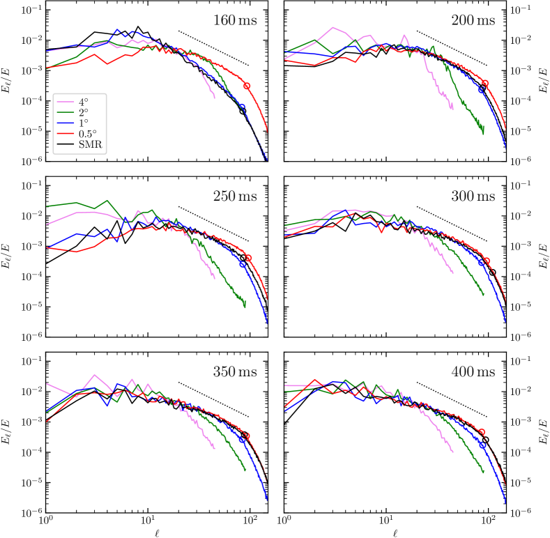
Figure 12: Normalized spectra of the nonradial turbulent kinetic energy for the HTCL model set with $L_{\nu,52}=4$, measured between the gain radius and the minimum shock radius. The spectra are averaged over 10 km around $R_{0}$ and a time interval of 5 ms. Open circles mark the beginning of the dissipation range, $\ell_{\mathrm{diss}}$. The dotted lines indicate the $(-5/3)$-power-law slope expected for Kolmogorov turbulence in the inertial range. At 300 ms the spectra of the simulations with SMR grid and 0.5^∘ resolution become very similar, whereas at earlier times the spectra of SMR and 1^∘ simulations are more similar. This is fully compatible with the growing resolution of the SMR grid as the shock moves to larger radii.

In Fig. 12, we present energy spectra for the HTCL simulations with $L_{\nu,52}=4$ at certain times after core bounce. The spectra are measured at a radius $R_{0}$ between the angle-averaged gain radius, $R_{\mathrm{gain}}$, and the minimum shock radius, i.e.,

$$R_{0}=\frac{1}{2}\left(R_{\mathrm{gain}}+\min(R_{\mathrm{sh}})\right).$$ (20)

This choice assures that we do not include contributions from pre-shock material in our analysis. In order to smooth the data, we computed volume-weighted spatial averages of the energy spectra in the range $R_{0}\pm 5\,\mathrm{km}$ with an additional time-averaging in the interval $t\pm 2.5\,\mathrm{ms}$. To guarantee consistency, this procedure is also applied to the total kinetic energy density $E$ used for the normalization of the spectra.

From the angular grid resolution $\alpha$ of the 3D models, we can calculate the maximum multipole order $\ell_{\mathrm{max}}$ roughly according to $\ell_{\mathrm{max}}\approx 180^{\circ}/\alpha$. In the SMR simulation, $\alpha=1^{\circ}$ until $\sim$250 ms and $\alpha=0.5^{\circ}$ at later times, depending on the location of $R_{0}$ at the time when the spectrum is measured. However, due to round-off errors caused by limited computational accuracy, we are not able to compute spherical harmonics for $\ell>150$.

We can estimate the multipole order of the largest eddies $\ell_{L}$ from simple considerations about their size. The largest possible extension of turbulent vortex structures in the gain layer depends on the thickness of this shell and is

$$L=\left<R_{\mathrm{sh}}\right>-R_{\mathrm{gain}}.$$ (21)

As explained, for example, by Foglizzo et al. (2006), this can be translated into a multipole order according to

$$\ell_{L}=\frac{\pi R_{0}}{L}.$$ (22)

In the HTCL model set with $L_{\nu,52}=4$, we find $\ell_{\mathrm{L}}\sim 7-10$ during the phase of shock stagnation and $\ell_{\mathrm{L}}\sim 2-5$ towards the end of the simulations, which roughly coincides with the peak positions, $\ell_{\mathrm{peak}}$, of the kinetic power spectra. The multipole order of the largest eddies is nearly the same in all models, which is expected on grounds of the geometrical considerations for determining $\ell_{L}$.

An important aspect of Kolmogorov’s theory of turbulence is the presence of a $k^{-5/3}$ scaling in the inertial range of the energy spectrum. As we will show below, this translates into an $\ell^{-5/3}$ behavior in our decomposition. Hence, we added dotted lines of this slope in Fig. 12 to visualize the inertial range. The power spectra of our highest-resolved models are indeed close to a $(-5/3)$ power law for $\ell\gtrsim 30$, whereas for $10\lesssim\ell\lesssim 30$ the spectra are better described by a $(-1)$-power-law slope.

The value of $\ell$, above which kinetic energy is dissipated into internal energy, $\ell_{\mathrm{diss}}$, depends strongly on the grid resolution. It is visualized by a circle in Fig. 12 and also given in Table 2. In models with a resolution of $2^{\circ}$ or worse, we do not see any clear Kolmogorov regime. In better resolved models, the $\ell^{-5/3}$ behavior breaks down near $\ell\sim 100$, i.e. on an angular scale of about $2^{\circ}$, which means that dissipation sets in at the level of a few grid cells. According to Porter et al. (1998) and Sytine et al. (2000), the Piecewise Parabolic Method (PPM; Colella & Woodward, 1984) that is applied in Vertex-Prometheus dissipates kinetic energy below 2 to 12 grid cells, which is roughly consistent with our finding.

To sum up, the similarity of our numerical spectra to Kolmogorov’s theory of steady-state isotropic turbulence can be used as a motivation to (approximately) apply relations from this theory during phases of shock stagnation in our models. This seems justified in conditions where SASI does not introduce global large-amplitude variations by pumping kinetic energy into the lowest modes $\ell\lesssim 2$. In the high-resolution simulations of at least $1^{\circ}$, we see a clear separation between the inertial range with its characteristic slope of $-5/3$ and the dissipation range with a steeper decay.

5.2 Numerical viscosity and effective Reynolds number

The kinematic shear viscosity of the stellar medium in the gain layer is of the order of $0.1\,\mathrm{cm^{2}\,s^{-1}}$ and thus extremely low (e.g., Abdikamalov et al., 2015). Because the corresponding Reynolds numbers are extremely high, of order $\sim 10^{17}$, the evolution of the stellar plasma is described by the Euler equations instead of solving the Navier-Stokes equations, which include terms that account for viscous effects. However, the viscosity associated with the numerical scheme is many orders of magnitude larger than the physical viscosity of the stellar plasma (see., e.g., Müller, 1998). Interestingly, the interaction of neutrinos with matter in the gain layer produces a damping force on fluid motions—a neutrino drag—whose influence on the plasma flow is in the ballpark of the effects of numerical viscosity on the relevant scales (see Appendix B for a derivation and discussion of the neutrino drag in detail).

As in all other state-of-the-art core-collapse supernova models, we rely on the implicit large eddy simulation (ILES; Grinstein et al., 2007) paradigm. It assumes that dissipative effects on the smallest scales are implicitly accounted for by the numerical viscosity. Instead of solving filtered hydrodynamic equations and creating a sub-grid model for the dissipation of kinetic energy (Boris et al., 1992), the ILES approach assumes that such a sub-grid model is implicitly included at the level of the grid cell size.

Estimating the effective viscosity of a numerical scheme, $\nu_{\mathrm{N}}$, is difficult. It depends not only on the algorithm itself, but also on its implementation. Even if the numerical viscosity is known for one simulation code, it is not justified to assume an equal viscosity for all codes that make use of the same algorithm for treating the hydrodynamics. Consequently, the numerical viscosity and the effective Reynolds number must be determined for every code separately in order to estimate the influence of dissipative effects. This can only be achieved by measuring characteristic quantities from the output data.

In the following two sections, we will discuss two methods for determining the numerical viscosity and the effective Reynolds number from properties of the kinetic energy spectrum. Both approaches will be applied to our 3D simulations. The first procedure was proposed by Abdikamalov et al. (2015), while the second method has been developed by us and was presented in Melson (2016) before. As in the previous section, the energy spectra are averaged over $10\,\mathrm{km}$ and $5\,\mathrm{ms}$, and measured at a radius $R_{0}$ halfway between the angle-averaged gain radius and the minimum shock radius.

5.2.1 Based on the Taylor microscale

The method of Abdikamalov et al. (2015) is based on determining the so-called Taylor microscale, which is given by (Frisch, 1995; Pope, 2000)

$$\lambda=\sqrt{\frac{5E}{Z}},$$ (23)

where $E$ is the total kinetic energy density of nonradial fluid motions,

$$E\approx\sum_{\ell=0}^{\ell_{\mathrm{max}}}E_{\ell},$$ (24)

and $Z$ is the enstrophy, which can be approximated by

$$Z\approx\frac{1}{R_{0}^{2}}\sum_{\ell=0}^{\ell_{\mathrm{max}}}\ell(\ell+1)\,E_{\ell}.$$ (25)

For the upper bound $\ell_{\mathrm{max}}$, Abdikamalov et al. (2015) picked a value of $120$, while we calculate it from the angular resolution of the model.

The Taylor microscale $\lambda$ has no direct physical interpretation. It is situated somewhere between the characteristic scale of the smallest eddies—the Kolmogorov scale—and the size of the largest structures (Pope, 2000).

Abdikamalov et al. (2015) derived a relation for the effective Reynolds number,

$$\mathrm{Re}=5\frac{\tilde{L}^{2}}{\lambda^{2}},$$ (26)

which is, however, not fully consistent with the literature. Commonly, a factor of $10$ (Pope, 2000; Schmidt, 2014) or even $15$ (Tennekes & Lumley, 1972) instead of $5$ is applied. Nevertheless, in order to compare with the results of Abdikamalov et al. (2015), we also use their factor $5$ here. At the end of this section, we will further discuss this issue.

The size of the energy-containing eddies $\tilde{L}$ is calculated by Abdikamalov et al. (2015) from the energy spectrum according to (motivated by Eq. (22))

$$\tilde{L}=\pi R_{0}\left(1+\frac{1}{E}\sum_{\ell=0}^{\ell_{\mathrm{max}}}\ell\,E_{\ell}\right)^{-1}.$$ (27)

Finally, the kinematic numerical viscosity can be determined from the fundamental relation

$$\nu_{\mathrm{N}}=\frac{v_{0}\tilde{L}}{\mathrm{Re}}.$$ (28)

The characteristic velocity $v_{0}$ of the largest eddies is deduced from the total kinetic energy density (Eq. (17)) by

$$v_{0}^{2}\equiv\frac{1}{4\pi}\int\mathrm{d}\Omega\,\left(v_{\theta}^{2}+v_{\phi}^{2}\right)\approx\frac{E}{2\pi\rho_{0}}.$$ (29)

Note that in addition to $E$, also the density $\rho_{0}$ is averaged over a radial shell defined by $R_{0}\pm 5\,\mathrm{km}$ and a time interval of $t\pm 2.5\,\mathrm{ms}$.

The method of Abdikamalov et al. (2015) suffers from the uncertainty in Eq. (26) and in the scale defined in Eq. (27). Their application is debatable, because there might be factors of 2 or even 3 missing. This issue will be discussed later in this section. Furthermore, this approach yields Reynolds numbers being implausibly low and showing only a weak resolution dependence (see Table 2), which suggests a marginally turbulent flow for all resolutions tested, in obvious conflict with the situation observed in Figs. 5 and 6, and the presence of a Kolmogorov-like power spectrum over roughly one order of magnitude of $\ell$ in Fig. 12.

For the reasons mentioned, we have developed a different procedure, which yields more realistic values of the numerical viscosity and the effective Reynolds number.

5.2.2 Based on the energy dissipation rate

Our method for measuring the numerical viscosity and the Reynolds number is based on more fundamental properties of the turbulent energy cascade. In the inertial range, the kinetic energy spectrum only depends on the specific energy dissipation rate $\varepsilon$ and is given by (Landau & Lifshitz, 1987; Pope, 2000)

$$\mathcal{E}_{k}=C\,\varepsilon^{2/3}\,k^{-5/3},$$ (30)

where $\mathcal{E}_{k}\,\mathrm{d}k$ is the specific turbulent kinetic energy of the fluid in the interval $[k,k+\mathrm{d}k]$.

In order to be consistent with the literature, we employ the spectrum of the specific kinetic energy as defined in Eq. (18) rather than that of the kinetic energy density. The factor $C$ is a universal constant of $C=1.62$ and independent of the Reynolds number (Sreenivasan, 1995; Yeung & Zhou, 1997).

Since we decompose the spectrum by making use of spherical harmonics, it must be written as a function of the multipole order $\ell$ instead of the wave number $k$. This transformation reads

$$k=\frac{\sqrt{\ell(\ell+1)}}{R_{0}}\approx\frac{\ell}{R_{0}},$$ (31)

where the latter approximation is valid for sufficiently high values of $\ell$. The energy spectrum as a function of $k$,

$$\mathcal{E}_{k}\,\mathrm{d}k=C\,\varepsilon^{2/3}\,k^{-5/3}\,\mathrm{d}k,$$ (32)

can then be written as

$$\mathcal{E}_{\ell}\,\mathrm{d}\ell=C\,\varepsilon^{2/3}\,R_{0}^{5/3}\ell^{-5/3}\,\frac{\mathrm{d}\ell}{R_{0}}.$$ (33)

From this relation, we obtain an equation for the specific energy dissipation rate,

$$\varepsilon(\ell)=\sqrt{\frac{\mathcal{E}_{\ell}^{3}\,\ell^{5}}{R_{0}^{2}\,C^{3}}},$$ (34)

which allows for directly measuring its value from the spectrum, using Eq. (18) for $\mathcal{E}_{\ell}$ and Eq. (20) for $R_{0}$. Together with the specific enstrophy $\mathcal{Z}$ calculated approximately (becoming exact for $\ell_{\mathrm{max}}\longrightarrow\infty$) according to

$$\mathcal{Z}\approx\frac{1}{R_{0}^{2}}\sum_{\ell=0}^{\ell_{\mathrm{max}}}\ell(\ell+1)\,\mathcal{E}_{\ell},$$ (35)

we can determine the numerical viscosity from the equation (Tennekes & Lumley, 1972; Pope, 2000)

$$\nu_{\mathrm{N}}=\frac{\varepsilon}{2\mathcal{Z}}.$$ (36)

Note that the enstrophies defined in Eqs. (25) and (35) are connected to each other by the relation $Z\approx\rho_{0}\mathcal{Z}$.

The question arises, at which multipole order $\ell$ the energy dissipation rate should be measured for our purposes. If ideal Kolmogorov turbulence would apply, $\varepsilon$ would actually by constant in the inertial range. Because of deviations from this perfect Kolmogorov case, the most conservative approach is taking the peak value of $\varepsilon$ to evaluate Eq. (36), since we want to maximize our estimate of the numerical viscosity, which is known to be large. In practice, however, the spectra $\varepsilon(\ell)$ turn out to possess a very broad maximum, compatible with the Kolmogorov-like behavior.

Ultimately, we can calculate the effective Reynolds number as

$$\mathrm{Re}=\frac{v_{0}L}{\nu_{\mathrm{N}}},$$ (37)

where $L$ is taken from Eq. (21) and $v_{0}$ is the characteristic velocity of the largest eddies given by (see Eq. (19))

$$v_{0}^{2}=\frac{1}{2\pi}\sum_{\ell=0}^{\infty}\mathcal{E}_{\ell}\approx\frac{1}{2\pi}\sum_{\ell=0}^{\ell_{\mathrm{max}}}\mathcal{E}_{\ell}.$$ (38)

In contrast to the previous method, $L$ is assumed to be equal to the radial thickness of the gain layer (Eq. (21)). The values of $v_{0}$ obtained with Eqs. (38) and (29) are extremely similar (see Table 2).

5.2.3 Comparison of the methods

Table 2: Numerical Reynolds numbers and corresponding numerical viscosities evaluated using the AOR+ and MKJ methods for the 3D simulations of the HTCL model set with $L_{\nu,52}=4$.

		Abdikamalov et al. (2015, AOR+)				This work (MKJ)
160	$4^{\circ}$	(41)	(0.05)	134	0.02	(40)	(0.02)	46	0.02	-	141
	$2^{\circ}$	(50)	(0.03)	87	0.02	(60)	(0.01)	46	0.02	-	141
	$1^{\circ}$	47	8.4	99	3.9	87	2.6	56	4.0	83	140
	$0.5^{\circ}$	58	5.7	61	5.4	195	1.8	65	5.5	93	144
	SMR ($1^{\circ}$)	43	11.0	103	4.6	55	4.8	56	4.7	85	141
200	$4^{\circ}$	(35)	(0.6)	137	0.2	(12)	(0.6)	45	0.2	-	139
	$2^{\circ}$	(46)	(0.6)	96	0.3	(21)	(0.6)	44	0.3	-	139
	$1^{\circ}$	54	6.8	68	5.3	153	2.2	61	5.4	86	141
	$0.5^{\circ}$	58	5.9	57	5.9	199	1.9	64	6.0	93	142
	SMR ($1^{\circ}$)	59	6.4	68	5.6	163	2.1	61	5.7	88	141
225	$4^{\circ}$	(18)	(1.2)	97	0.2	(10)	(0.9)	41	0.2	-	134
	$2^{\circ}$	22	6.0	83	1.6	13	5.6	43	1.6	-	134
	$1^{\circ}$	54	6.1	67	4.9	132	2.1	57	5.0	81	137
	$0.5^{\circ}$	59	5.5	54	6.0	197	1.8	59	6.1	97	138
	SMR ($1^{\circ}$)	57	6.4	66	5.5	129	2.5	57	5.6	83	137
250	$4^{\circ}$	(39)	(0.8)	159	0.2	(48)	(0.4)	92	0.2	-	161
	$2^{\circ}$	39	4.1	124	1.3	46	2.6	92	1.3	-	160
	$1^{\circ}$	54	6.8	77	4.7	230	2.2	106	4.8	85	163
	$0.5^{\circ}$	60	5.3	62	5.1	306	1.8	109	5.1	96	165
	SMR ($0.5^{\circ}$)	61	6.0	73	5.0	279	2.0	108	5.0	86	163
300	$4^{\circ}$	36	25.5	173	5.3	101	8.8	168	5.3	-	182
	$2^{\circ}$	47	19.6	137	6.6	183	7.3	198	6.7	-	197
	$1^{\circ}$	55	11.4	97	6.4	368	3.8	216	6.5	86	206
	$0.5^{\circ}$	59	9.3	83	6.7	443	3.3	219	6.7	96	204
	SMR ($0.5^{\circ}$)	62	10.2	92	6.9	515	3.0	217	7.0	110	207
350	$4^{\circ}$	34	33.6	184	6.2	97	13.2	206	6.2	-	198
	$2^{\circ}$	47	23.3	150	7.3	322	6.4	281	7.3	-	220
	$1^{\circ}$	56	15.9	121	7.3	413	5.6	312	7.4	84	238
	$0.5^{\circ}$	57	12.8	96	7.6	631	3.8	313	7.7	92	229
	SMR ($0.5^{\circ}$)	63	13.3	109	7.7	535	4.3	293	7.8	88	231
400	$4^{\circ}$	35	35.8	172	7.3	132	11.5	208	7.3	-	175
	$2^{\circ}$	45	27.6	168	7.3	286	9.5	362	7.5	-	240
	$1^{\circ}$	58	20.8	156	7.6	549	6.2	437	7.8	88	279
	$0.5^{\circ}$	59	14.5	111	7.7	682	4.6	400	7.9	86	250
	SMR ($0.5^{\circ}$)	63	14.6	111	8.3	715	4.1	348	8.4	94	233

We present the Reynolds numbers and numerical viscosities calculated with the two methods described above in Table 2. The procedure of Abdikamalov et al. (2015) based on the Taylor microscale is denoted by AOR+ and compared to our method (denoted by MKJ) based on the energy dissipation rate.

The Reynolds numbers computed with the AOR+ method have only a very weak resolution dependence and exhibit only marginal changes after 200 ms post bounce in models with developed postshock turbulence. Note that in Table 2, numbers for Re and $\nu_{\mathrm{N}}$ are set in parentheses when the corresponding models had not yet developed such turbulent conditions in the postshock layer.

While the grid spacing in our model with $0.5^{\circ}$ angular resolution is a factor of eight finer in each angular direction than in the $4^{\circ}$ case, the Reynolds number for the AOR+ estimate increases only by a factor of $\sim$2 to values around 60. Such values of the Reynolds numbers seem to be too low in view of the well developed Kolmogorov-like turbulent cascade witnessed over roughly one order of magnitude of $\ell$ in Fig. 12, and they appear to be underestimated also in comparison to other results discussed in the literature. Based on a systematic study of Porter & Woodward (1994), Keil et al. (1996), for example, estimated values of $\mathrm{Re}\sim 1000$ for 2D simulations with $1.5^{\circ}$ resolution performed with Prometheus.

With our method (MKJ), we obtain values for $\mathrm{Re}$ that are more consistent with the observed flow behavior in the neutrino-heated postshock layer. During the shock-stagnation phase (which lasts until $\sim$230 ms after bounce), Reynolds numbers of up to $\sim$200 are reached in the models with at least $1^{\circ}$ angular resolution.

From 200 ms to 225 ms, the Reynolds numbers remain relatively constant for fixed resolution in our analysis. This indicates that the turbulent cascade is in steady-state conditions during this period. We do not witness any evidence that the scaling relations of classical turbulence theory might not be applicable here. After 250 ms, the shock expansion leads to an increasing value of $L$ and a corresponding increase of the Reynolds number, in contrast to values obtained with the AOR+ approach.

With increasing angular resolution of the simulations, we see also increasing Reynolds numbers because of decreasing values of the numerical viscosity, as expected from the point of view that better resolution should reduce viscous damping of the turbulent flow by dissipative effects associated with the grid discretization. Models that do not follow this trend have not yet fully developed turbulence in the postshock layer, for which reason the MKJ estimates become unreliable. The corresponding numerical results are set in parentheses in Table 2. The numbers of Re and $\nu_{\mathrm{N}}$ for the SMR models are close to those models with fixed resolution that match the resolution of the SMR models at the radius of evaluation, $R_{0}$.

The two approaches, AOR+ and MKJ, described above yield Reynolds numbers and numerical viscosities that differ significantly. In order to analyze why this is the case, we divide Eqs. (26) and (28) by Eqs. (37) and (36), respectively, i.e., we divide the values calculated with the method of Abdikamalov et al. (2015, AOR+) by the values obtained with our procedure (MKJ). The ratio of the Reynolds numbers reads

$$R_{\mathrm{Re}}\equiv\frac{\mathrm{Re}^{\mathrm{AOR+}}}{\mathrm{Re}^{\mathrm{MKJ}}}=\frac{\tilde{L}^{2}Z/E}{2\mathcal{Z}v_{0}L/\varepsilon}=\frac{\varepsilon\tilde{L}^{2}}{4\pi v_{0}^{3}L},$$ (39)

and the ratio of the numerical viscosities is given by

$$R_{\nu_{\mathrm{N}}}\equiv\frac{\nu_{\mathrm{N}}^{\mathrm{AOR+}}}{\nu_{\mathrm{N}}^{\mathrm{MKJ}}}=\frac{v_{0}E/\tilde{L}Z}{\varepsilon/2\mathcal{Z}}=\frac{4\pi v_{0}^{3}}{\varepsilon\tilde{L}},$$ (40)

where in addition to the mentioned equations we also made use of Eqs. (23) and (29), and of $Z\approx\rho_{0}\mathcal{Z}$. Ideally, both quantities —$R_{\mathrm{Re}}$ and $R_{\nu_{\mathrm{N}}}$— should be unity. However, the ratio $R_{\mathrm{Re}}$ can be as small as 0.1, while $R_{\nu_{\mathrm{N}}}$ can reach values of 3–4 (see Table 2). Since the estimates of $v_{0}$ from both methods are basically identical and $\tilde{L}$ and $L$ do not differ by more than 2–3 in most cases (see Table 2), we conclude that our MKJ appoach yields lower estimates for the numerical energy-dissipation rate, $\varepsilon$. In other words, the method of AOR+ intrinsically overestimates the numerical energy-dissipation rate.

In our approach, the energy-dissipation rate $\varepsilon$ is directly measured from the energy spectrum according to Eq. (34). The only term in Eq. (34) being not precisely known is the constant $C$. However, it was determined to satisfactory accuracy and even the largest possible reduction of $C$ within the error bars mentioned by Sreenivasan (1995) would enhance $\varepsilon$ only by $18\%$. For the proposed best value of $C$, we have measured the peak amplitude of $\varepsilon(\ell)$ to maximize the numerical viscosity. Hence, we conclude that a significant underestimation of the energy dissipation rate is unlikely.

Another ambiguity concerns the length scales of the relevant turbulent eddies. The values in Table 2 suggest that $\tilde{L}$ according to Abdikamalov et al. (2015) is sometimes too large, especially in cases where $\tilde{L}$ is larger than the gain-layer width. Our calculated values of $L$ are often more than a factor of two different from $\tilde{L}$ (smaller at early times and larger towards the end of our simulations). These values of $L$ represent the true size of the largest eddies, which marks an upper limit for the energy-containing eddy scale, i.e. for $\tilde{L}$. Determining the relevant length scale from the spectral shape as done by Abdikamalov et al. (2015) seems problematic, because $\tilde{L}$ varies significantly with grid resolution, whereas on grounds of physics one would expect that the size of the energy-containing eddies, corresponding to the energy-weighted mean of the multipole order, should hardly depend on the grid resolution. Since the energy-injection scale is determined by the thickness of the layer of main neutrino-energy deposition, this scale should be very similar between all simulations within the HTCL model set. Also the location of the peak of the power spectrum is fairly similar in all models with fully developed turbulence, as can be seen in Fig. 12. Moreover, solely the radial thickness of the gain layer constrains the diameter of the largest turbulent structures, which is exactly the motivation for our choice of $L$ in Eq. (21). For all these reasons, it does not seem plausible that the relevant scale for estimating the Reynolds number, as in the approach of Abdikamalov et al. (2015), exhibits a strong variation with the angular resolution of the model.

We therefore suspect that the misjudgment of the relevant turbulent eddy scale in the AOR+ method might be the underlying cause for the counterintuitively weak variation of the Reynolds number with angular resolution and for the strange fact that Re is basically independent of the growing radial diameter of the postshock layer at later times (Table 2). Furthermore, note that due to the quadratic dependence in Eq. (26), the Reynolds number in the AOR+ approach is more sensitive to the length scale than in our method.

Besides these considerations of over- and underestimated eddy scales, the numerical constant used in the calculations of the Reynolds numbers in the approach of Abdikamalov et al. (2015) appears to be too low in general. The factor $5$ in Eq. (26) is disputable, because it is smaller than what is reported in the literature. Tennekes & Lumley (1972) formulated Eq. (26) in a different way, namely as

$$\mathrm{Re}=\frac{15}{A}\frac{\tilde{L}^{2}}{\lambda^{2}},$$ (41)

where $A$ is an “undetermined constant” of order unity. Pope (2000) and Schmidt (2014) used $A=3/2$, whereas Abdikamalov et al. (2015) and also Couch & Ott (2015) applied $A=3$. Obviously, there is some ambiguity with respect to the value of this constant. The Reynolds numbers of Abdikamalov et al. (2015) are therefore likely to be more than a factor of two too small. This highlights an important aspect of turbulence theory. Many equations are obtained from self-similarity considerations and therefore based only on proportionalities. Scaling factors are then derived from further assumptions or they remain undetermined.

Our approach to calculate the numerical viscosity relies on the fundamental relations of Kolmogorov’s theory and avoids the usage of other equations. Although our values computed for the Reynolds numbers might be slightly overestimated due to their sensitive dependence on $v_{0}$ and $L$, the numerical viscosities deduced from the measured turbulent power spectra with our formalism are not subject to corresponding uncertainties and can therefore be considered as solid measures, provided that turbulence is fully developed and that Kolmogorov’s theory is applicable.

6 Discussion

The main result of our resolution study, namely that higher angular resolution is beneficial for stronger shock expansion and shock revival in 3D simulations, is in contradiction with results of a previous investigation by Hanke et al. (2012), whose 3D models with higher angular resolution showed the tendency to explode later or not at all, in spite of the success of lower-resolution cases.

Both generations of simulations differ in several aspects (see Section 2.2), namely in the use of slightly different versions of the high-density equation of state of Lattimer & Swesty (1991), minor modifications in the neutrino-cooling description, general relativistic corrections in the gravitational potential instead of the Newtonian gravity used by Hanke et al. (2012), and the replacement of the previously employed spherical polar grid by the axis-free Yin-Yang grid. While the first three aspects have the effect of changing the value of the neutrino luminosity needed to trigger shock revival, they cannot explain the opposite dependence of the explosion behavior on resolution.

The crucial change was the introduction of the Yin-Yang grid, which allows for numerically cleaner resolution tests due to less grid-associated effects. The polar axis of regular spherical coordinate grids does not only possess a coordinate singularity that can induce artifacts, but also the nonuniform cell sizes of the angular grid with smaller azimuthal cells near the polar axis (and thus lower numerical viscosity) may have perturbative effects. In all 3D simulations with a standard polar grid, we can observe postshock convection appearing earlier near the polar axis and becoming first visible by a buoyant plume that expands along the axis and deforms the shock. This shock deformation creates vorticity and entropy perturbations in the postshock flow and thus triggers the development of neutrino-driven convection or SASI mass motions, depending on which of these instabilities is favored to grow faster by the physical conditions. Therefore, in all of the 3D simulations performed by Hanke et al. (2012), even in the runs with the lowest angular resolution of $3^{\circ}$, shock asphericity and nonradial kinetic energy were found to rise already at 80–130 ms after bounce. This is in sharp contrast to our current set of models, where due to numerical viscosity in the low-resolution ($2^{\circ}$ and $4^{\circ}$) cases, nonradial kinetic energy in the gain layer does not appear on a visible level before 200 ms after bounce (see Figs. 7, 8, and 9).

For this reason, the shock expansion and revival in the simulations by Hanke et al. (2012) were strongly influenced by the presence of the polar grid axis and the variable cell sizes of the angular grid, which had the consequence of enhancing nonradial mass motions in the postshock region. With higher resolution (in 3D it could be improved only moderately to 2^∘ instead of 3^∘) this influence seems to have lost strength, which is why the better resolved models showed a reduced tendency to produce explosions. In the models of the current study the angular cells of the Yin-Yang grid are basically uniform and a polar axis is absent. Therefore, grid-induced irregularities occur on a much lower level and do not determine the development of nonradial flows in the postshock layer. Consequently, our models with higher angular resolution and correspondingly lower numerical viscosity exhibit stronger turbulence, which supports shock expansion and fosters explosions.

From this discussion another consequence arises: Comparisons of our results based on the Prometheus code to resolution studies discussed in the literature require great caution and are by no means straightforward. Code-specific aspects such as the order of the employed hydro solver and different grid setups used by different groups could play a role. It is, for example, conspicuous that the result of Hanke et al. (2012) of low resolution yielding more favorable conditions for explosions in 3D, was reproduced by studies that employed Cartesian grids with static or adaptive mesh refinement (AMR) (Couch & O’Connor, 2014; Couch & Ott, 2015; Roberts et al., 2016) or with a combination of overlapping grid blocks in a cubed-sphere multi-block AMR system (Abdikamalov et al., 2015), or, as in the study by Radice et al. (2016), with a spherical mesh but a computational domain that was constrained to an octant with inner and outer radial boundaries, using periodicity in the angular directions and a reflecting boundary condition at the inner boundary. While possible artificial effects of such a constrained simulation volume with polar coordinates have not been explored yet (Roberts et al. 2016 and O’Connor & Couch 2018 also investigated cases with octant symmetry but employed Cartesian AMR), it is known that Cartesian grids impose perturbations on radial flows. Even the boundaries between AMR or grid domains with different resolutions or geometry could have problematic numerical consequences, similar to what we observed at the resolution boundaries of our SMR grid. One might speculate that Cartesian grids with higher resolution create a lower level of numerical noise, thus leading to weaker driving of postshock turbulence and therefore less beneficial conditions for explosions. This might be the reason why Cartesian setups with lower resolution produced faster explosions, while the authors of the corresponding papers attributed this result to greater nonradial kinetic energy on the lowest-order multipolar scales because of suppressed cascading of turbulent energy to high-$\ell$ scales.

While more extended speculations about the possible impact of grid effects do not appear very productive in default of investigations of how different codes with different grid setups perform on the same well-controlled test problems, it is clear from all of what was said above that Cartesian results cannot be contrasted with results from polar grids by simply identifying the size of the Cartesian cells with an effective angular resolution of a spherical grid (see, e.g., Couch, 2013; Ott et al., 2013; Abdikamalov et al., 2015; Couch & Ott, 2015; O’Connor & Couch, 2018). Numerical artifacts associated with Cartesian grids and polar grids are too different and may even govern the solutions. Moreover, changes of the resolution in radial and angular directions can have different consequences (see Hanke et al., 2012), but in Cartesian simulations they cannot be varied independently. Correspondingly, in 3D supernova simulations with Cartesian grids the minimum cell size in the vicinity of the steep density decline near the surface of the proto-neutron star is typically around 500 m or even more (e.g., Couch, 2013; Couch & O’Connor, 2014; Couch & Ott, 2015; Dolence et al., 2013; Ott et al., 2013; Kuroda et al., 2016; Roberts et al., 2016; O’Connor & Couch, 2018), similar to what was employed in recent 3D calculations with the Fornax code using spherical (dendritic) coordinates (Vartanyan et al., 2019; Burrows et al., 2019). In contrast, in applications of the Prometheus code with simplified neutrino treatment as well as the Prometheus-Vertex code with elaborate and computationally expensive neutrino transport, the radial resolution in the same region is chosen to be much finer, and it is improved with time as the density gradient gradually steepens, to become as good as 50–100 m after 500 ms post bounce. It is evident that more studies, including direct comparisons of different codes with different grids, applied on the same test problems, are needed to disentangle numerical and physical effects in the growing suite of 3D supernova models.

7 Summary and Conclusions

7.1 Summary

In this paper, we investigated the resolution dependence and convergence properties of 3D simulations with the Prometheus-Vertex supernova code. Because of limited computational resources, previous neutrino-hydrodynamics calculations with this code, in particular also the successful 3D explosion models reported by Melson et al. (2015a, b) and Summa et al. (2018), were conducted with an angular cell size of $2^{\circ}$ for the employed polar and Yin-Yang grids. However, in regions where hydrodynamic instabilities and turbulent effects play a role, in particular in the convectively unstable neutrino-heating layer behind the stalled supernova shock, more angular resolution is desirable. Therefore we introduced a new static mesh refinement (SMR) procedure in our code, which can compensate the decreasing resolution (in terms of absolute scales) associated with the geometrical widening of the lateral and azimuthal grid zones with growing distance from the coordinate center. This SMR grid allows us to increase the number of angular grid cells in defined radial regions without equally increasing the number of angular zones (also termed radial “rays”) for the ray-by-ray-plus neutrino transport. In the neutrino-heating layer and farther outside, where neutrinos are nearly decoupled from the stellar background (the optical depth of these layers is typically below 0.2), the use of less transport rays than angular zones in the hydrodynamics solver is a viable approximation. Such an approach saves considerable amounts of computer time because the transport module accounts for the dominant part of the required computational resources.

The results presented here show, however, that the SMR technique comes with some downsides. While in the case of a robustly exploding 9 $M_{\odot}$ progenitor we did not observe any significant differences between simulations with uniformly spaced low-resolution ($3.5^{\circ}$) grid and a high-resolution SMR setup, a $20\,M_{\odot}$ model that evolved along the borderline between explosion and failure showed undesirable sensitivity to the chosen grid setup. It developed an explosion with uniform $2^{\circ}$ angular resolution, whereas it did not succeed to blow up when the SMR grid was used. The SMR model failed despite the fact that its average shock radius was transiently larger (reaching up to 170–180 km) than in the case with uniform angular grid, where it was only $\sim$150 km.

We took this finding as a motivation for a systematic study that was intended to clarify the underlying numerical reasons and to disentangle the consequences of higher angular grid resolution from effects associated with the SMR method. To achieve this goal with acceptable investment of computing time, we replaced the Vertex neutrino-transport treatment by a simplified heating and cooling (HTCL) scheme and set up 20 $M_{\odot}$ simulations such that the supernova shock reached a stagnation radius of about 170–180 km as it did temporarily in the 20 $M_{\odot}$ SMR model with full-fledged neutrino transport. All exploding models in this carefully controlled study with SMR grid and uniform resolutions of $4^{\circ}$, $2^{\circ}$, $1^{\circ}$, and $0.5^{\circ}$ experienced shock revival (or temporary shock expansion) at the same time. This fact enabled a particularly clean and conclusive investigation of the influence of varied angular resolution on the shock evolution.

As in the simulations with full neutrino transport, we observed that higher resolution leads to a slightly larger shock stagnation radius. Moreover, better resolved simulations do not only display a considerably earlier onset of postshock convection in the neutrino-heating layer but also show more fine structure in the postshock flow once turbulent convection has developed. This corresponds to differences in the normalized turbulent power spectra with relatively less kinetic energy on large multipolar scales ($\ell\lesssim 10$) and relatively more power on small scales, roughly following a Kolmogorov-like $\ell^{-5/3}$ power law from $\ell\sim 30$ up to the dissipation scale around $\ell\sim 100$ in all cases where the resolution is better than $\sim$1^∘. Low resolution obviously delays the growth of nonradial postshock instabilities, and the associated higher numerical viscosity prevents cascading of kinetic energy from the largest scales to turbulent vortex flows on smaller scales. This goes hand in hand with lower nonradial kinetic energy and a reduced efficiency for conversion of neutrino heating to turbulent kinetic energy. During this phase the highest-resolved $0.5^{\circ}$ model still exhibits noticeable differences compared to the SMR and $1^{\circ}$ simulations.

Shock expansion in reaction to the arrival of the infalling silicon/silicon+oxygen interface at the stagnant shock finally enables the onset of postshock convection in all of our HTCL models, also in the coarse-resolved ones, because the decreased accretion velocity in the postshock flow allows buoyant plumes to rise outward. In this phase, the shock develops runaway expansion in all cases except the $4^{\circ}$-degree runs. The expansion velocity of the shock clearly shows a monotonic dependence on the resolution with possible convergence at about $1^{\circ}$. Simulations that are closer to the explosion threshold are more sensitive to resolution changes. Models with a resolution of at least $1^{\circ}$ develop similar fluid structures. The SMR run resembles simulations with a uniform resolution of $0.5^{\circ}$ in this respect. Only towards the end of the SMR simulation, the expansion velocity of the shock drops slightly below the value of the $1^{\circ}$ and $0.5^{\circ}$ models. Our analysis revealed that this effect is caused by the dissipation of kinetic energy at the interfaces of layers with different angular resolutions in the SMR setup. Downflows propagating from the finer grid to the layer with coarser resolution under the constraint of total energy conservation lose kinetic energy that is transformed into internal energy. This leads to reduced pressure support of the expanding shock because thermal energy provides pressure with an adiabatic index of $4/3$, whereas turbulent pressure connects to turbulent kinetic energy with an equivalent adiabatic index of 2 (see Radice et al., 2015).

The bottom line is that the dynamical evolution of our 20 $M_{\odot}$ HTCL models during the shock stagnation and shock revival phases is basically identical in 3D simulations with $1^{\circ}$, $0.5^{\circ}$, and SMR grid, despite remaining resolution-dependent differences in various measures of turbulence (e.g., the initial growth of convective activity, the saturation level of the nonradial kinetic energy during shock stagnation, and the detailed shape of the normalized mode spectrum of the kinetic energy). Even the $2^{\circ}$ run follows closely when the shock expansion sets in, while the $4^{\circ}$ model exhibits a visibly weaker shock expansion because higher numerical viscosity attenuates turbulent mass motions and reduces the turbulent kinetic energy. A similar effect, though less extreme, could also be witnessed at the interfaces of domains of different angular resolution in our SMR setup, where kinetic energy of flows crossing boundaries from higher to lower resolution is converted to thermal energy. The grid resolution has a more sensitive influence in cases that marginally overcome the explosion threshold.

In order to quantify the influence of numerical viscosity, we introduced a method of calculation that is based on the energy dissipation rate measured directly from the turbulent energy spectrum. Our method differs from the approach used by Abdikamalov et al. (2015), who derived results based on the Taylor scale. We determined effective numerical Reynolds numbers for the postshock flow in our high-resolution ($0.5^{\circ}$, $1^{\circ}$, and SMR) runs of up to several hundred, and in our $2^{\circ}$ and $4^{\circ}$ models of a few dozens to a few hundred. Such values agree with previous rough estimates for simulations of proto-neutron star convection with the Prometheus code (Keil et al., 1996), and they are consistent with those reported by Handy et al. (2014). Our numerical viscosities, however, are lower by a factor of $\sim$2–4 compared to the results we obtained with the formalism of Abdikamalov et al. (2015), and our numerical Reynolds numbers are considerably higher (by up to a factor of $\sim$10) than those computed according to these authors. We consider our estimates as better compatible with the fine-structured vortex pattern witnessed in the convective postshock flow of our high-resolution models, which is mirrored by a near-Kolmogorov spectrum of the turbulent kinetic energy over an order of magnitude in the spherical harmonics modes $\ell$.

We also presented a detailed evaluation of neutrino-drag terms in the hydrodynamics equations for the conditions between neutrinosphere and supernova shock in Appendix B. Interestingly, the numerical Reynolds numbers of postshock turbulence even in our lowest-resolved simulations, which range between several 10 and some 100 on the relevant scales, are in the ballpark of the damping effects associated with neutrino drag acting on the flow in the gain layer. Concerns were expressed that current full-scale supernova models are severely underresolved and that much higher grid resolution is needed to describe the turbulent energy cascading in the convective postshock layer in order to reproduce the self-similar power-law spectrum of Kolmogorov’s classical theory in the inertial range despite numerical viscosity (Couch & Ott, 2015; Radice et al., 2016, 2018). Such reservations, however, must be confronted with the presence of neutrino drag in this region. Neutrino drag has a non-negligible influence on all structures in the postshock flow that are responsible for significant contributions to the turbulent kinetic energy. It is neither accounted for by the leakage schemes applied for neutrino energy and lepton sources in all previous resolution studies (e.g., Couch & O’Connor, 2014; Couch & Ott, 2015; Abdikamalov et al., 2015; Radice et al., 2016) nor by the simple heating and cooling treatment used in our work, but it requires the inclusion of neutrino-momentum transfer terms in the equation of motion (see Appendix B).

7.2 Conclusions

In our systematic resolution study, designed in a very careful way to avoid numerical perturbations (mainly grid-induced “noise” and fluctuations associated with neutrino effects) as much as possible, we witnessed a beneficial effect of higher angular resolution on shock revival. This can be understood by a lower level of numerical viscosity, allowing for higher turbulent kinetic energy because of reduced viscous damping and dissipation of nonspherical flows. Convergence of the overall shock dynamics in 3D seems to be approached at an angular resolution of about $1^{\circ}$, but simulations with a resolution of $2^{\circ}$ are not far off, despite the fact that properties characterizing turbulence, for example the exact shape of the turbulent energy spectrum and the scale when dissipation sets in, still exhibit differences when improving the resolution to $0.5^{\circ}$. Also in this context, our simulations with $1^{\circ}$ angular resolution match the requirements of convergence to a Kolmogorov-like behavior (at least for $\ell\gtrsim 30$) by displaying a clear separation of inertial range and dissipation range in the turbulent kinetic-energy spectra, contradicting a proposition by Radice et al. (2018) that these two length scales are usually merged in core-collapse supernova simulations and therefore misidentified.

The bottleneck effect pointed out by Radice et al. (2015, 2016, 2018), which is present in the turbulent energy spectra even for the highest feasible resolutions, seems to have a relatively minor influence on the overall shock evolution. Such a possibility was also admitted by Radice et al. (2016). This may be explained by the fact that most of the turbulent kinetic energy, which produces turbulent pressure to support shock expansion, is carried by vortex motions on large scales but not on the smallest scales near the dissipation regime.

The convergence of the supernova dynamics seen around $1^{\circ}$ angular resolution provides some back-up to the successful 3D explosion models computed with the Prometheus-Vertex and Alcar codes by Melson et al. (2015a, b), Summa et al. (2018), and Glas et al. (2019) with a resolution of $2^{\circ}$. Higher angular resolution has been found to be supportive of an explosion, and resolution-dependent differences are mostly relevant for cases whose postbounce evolution proceeds very close to the threshold between successful explosion and failure. Based on our estimates of the magnitudes of numerical viscosity and of neutrino drag acting on the flow in the gain layer, we infer that both effects are in the same ballpark for the numerical resolutions applied in the models of this work. Increasing the resolution significantly beyond an angular resolution of 1^∘–2^∘ is an exercise of direct relevance for the case of core-collapse supernovae only when neutrino viscosity (at high densities where neutrinos diffuse) and neutrino drag (outside of the diffusion regime) are taken into account.

Using our new SMR grid setup for improving the angular resolution in defined computational domains had the drawback that kinetic energy was converted to internal energy in flows crossing the borders from finer to coarser grid under the constraint of total energy conservation. In models evolving very close to the explosion threshold, this undesirable effect was found to weaken the explosion, whereas robustly exploding models remained unaffected. Finally, our result of higher angular resolution being favorable for explosion in 3D contradicts the trend seen by Hanke et al. (2012). The reason for this difference is the use of a polar grid in the previous simulations, whereas an axis-free Yin-Yang grid was applied in the current work. The presence of the polar-axis singularity and smaller azimuthal grid cells in the vicinity of the polar axis caused numerical artifacts that were stronger for lower-resolution runs. Correspondingly enhanced turbulent activity in the postshock region produced more favorable conditions for explosion in the lower-resolved 3D models of Hanke et al. (2012). In contrast, the cleaner setup of the resolution study presented here revealed the opposite behavior. Our findings that grid effects can have a severe influence on the solutions should also be taken as a clear warning that great caution is demanded when resolution studies based on Cartesian grids with AMR (e.g., Couch & O’Connor, 2014; Couch & Ott, 2015; Abdikamalov et al., 2015) or based on constrained volumes with radial and angular boundaries (e.g., the semiglobal setup considered by Radice et al., 2016) are interpreted. Boundary artifacts and unavoidable numerical noise imposed on radial flows on Cartesian grids, whose scale and amplitude differ when the resolution is varied, could affect the results and might provoke misleading trends.

Our work constitutes a very careful investigation of resolution effects in 3D supernova simulations with the Prometheus code for comparison with results and their interpretation in the literature. It suggests that previous studies revealed incorrect trends, namely opposite to our resolution-dependent results, because of numerical artifacts associated with the existence of a polar grid axis or numerical perturbations induced by Cartesian grids. “Realistic” simulations of stellar core collapse and explosions, however, are probably not seriously jeopardized by any of these numerical shortcomings, maybe not even by a moderate overestimation of numerical viscosity in the neutrino-heating layer due to the choice of modest spatial resolution, enforced by limited computational resources. The pre-collapse perturbations in the infalling stellar matter that are caused by fluctuations associated with convective shell burning in the progenitor stars (e.g., Couch & Ott, 2013; Müller & Janka, 2015; Couch et al., 2015; Müller et al., 2016; Yoshida et al., 2019; Yadav et al., 2019), provide a strong driving force of postshock turbulence, which is likely to easily dominate the damping effects of numerical viscosity in the currently best-resolved 3D supernova models (e.g., Müller et al., 2017, 2019).

Appendix

A Static mesh refinement

Both the spherical polar grid and the Yin-Yang grid have a common disadvantage. The surface element $\mathrm{d}A=r^{2}\,\sin\theta\,\mathrm{d}\theta\,\mathrm{d}\phi$ is proportional to the radius squared. For a given constant angular resolution, the effective size of the grid cells grows with increasing radius. Fine angular resolution near the grid center can impose severe constraints on the Courant-Friedrichs-Lewy (CFL) time step, while coarse resolution at large radii (behind the supernova shock) limits the possibility to resolve turbulent flows. Here, we present a static mesh refinement (SMR) technique, which compensates for the diverging structure of these spherical grids.

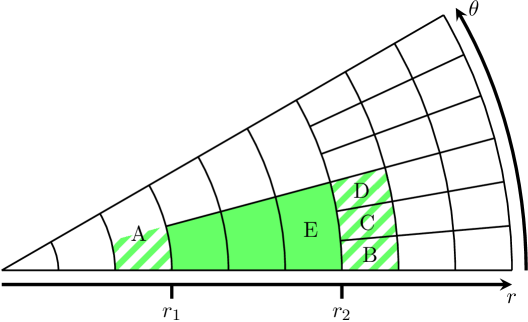
Figure A1: Example of a setup with static mesh refinement (SMR) in two dimensions. The angular resolution increases by a factor of $6$ from the center to the outer edge of the grid. The ghost cells for the green-shaded radial sweep between $r_{1}$ and $r_{2}$ are illustrated as green hatched areas. Note that unlike the exemplary setup shown in this figure, all supernova applications with SMR grid discussed in the main text were performed with doubling of the resolution in each angular direction at both SMR interfaces.

The SMR setup allows us to define certain radial intervals with different angular resolutions. An example for such a setup is given in Fig. A1 in two dimensions for coordinates $(r,\theta)$. Although this was chosen for the sake of simplicity here, the discussion is completely analogue to the 3D case, where it applies to both angular directions, $\theta$ and $\phi$. Let us define the angular resolution in Fig. A1 for $r<r_{1}$ as $\psi$. Then, the resolution between $r_{1}$ and $r_{2}$ is $2\psi$, and further refined to $6\psi$ for $r>r_{2}$.

Generally, arbitrary integer refinement steps and an arbitrary number of concentric layers can be chosen in our implementation. Note that the inner spherically symmetric volume, which is used in our simulations to allow for larger hydrodynamical time steps, can be understood as a special case with the lowest possible angular resolution corresponding to the whole sphere.

The radial locations of the refinement boundaries can be adjusted manually in our implementation at each restart of the code. Such a shift is motivated, for example, by a contraction of the gain radius that should roughly be followed by the grid setup.

Müller (2015) and Skinner et al. (2019) also implemented a similar setup, however, with the motivation of avoiding time-step constraints as the grid cells become smaller towards the grid singularities at the axis and at the origin. In their “dendritic” grid, they coarsen only the polar grid ($\theta$) to compensate for the diverging cell size with increasing radius. The azimuthal mesh ($\phi$) is coarsened towards the axis, which is not required in our setup when we use the axis-free Yin-Yang grid.

A.1 Treatment of the hydrodynamics

Generally, the SMR procedure only affects the radial direction. The computations of $\theta$ and $\phi$ sweeps remain unchanged. Besides the spherical polar grid, using the Yin-Yang grid is thus also possible and only requires a slight modification. As the angular resolution changes in the computational domain, the Yin-Yang ghost cell positions providing the boundary conditions for the angular sweeps are different for each refinement layer, which has to be considered when data is exchanged between both grid patches.

Radial sweeps are computed separately for every resolution layer. For an example, consider the green-filled grid cells in Fig. A1, for which the radial sweep should be calculated. Let us assume that one ghost cell is needed below and one above this sweep, depicted as green-hatched areas. On the lower side, the ghost cell data can directly be taken from cell A. This is because finite-volume methods generally assume that values in a cell always represent averages. At the upper end of the sweep, we need to average over cells B, C, and D to get the required data. Generally, averaging is required for the ghost cells located in the finer neighboring layer. This is the reason why only integer refinement steps are allowed in the SMR construction. Otherwise, computing the averages would be difficult and introduce additional interpolation errors.

A.2 Flux correction

If we naively used the averaged ghost cell data from the finer layer at the outer end of a radial sweep, numerical inaccuracies would occur resulting in the violation of conservation laws. In order to ensure exact conservation of the conserved quantities in our hydrodynamical scheme, a “flux correction” algorithm is applied acting on the outermost cell of each refinement region. We will explain this procedure with the aid of Fig. A1. Note that the flux correction is also done for the spherically symmetric innermost volume, which is usually employed in 3D to mitigate the time step constraints at the grid origin.

In our example illustrated in Fig. A1, the flux correction considers the interface between the cell E and the cells B, C, and D at $r_{2}$. After all radial sweeps have been calculated, the quantity $\mathcal{X}$—a placeholder for a conserved quantity in our hydrodynamical scheme—should be exactly conserved. The considered interface at $r_{2}$ is part of four different radial sweeps: the sweep between $r_{1}$ and $r_{2}$ containing the cell E, and the three sweeps beyond $r_{2}$ containing the cells B, C, and D. In the following, we discuss the different Riemann fluxes of $\mathcal{X}$ at the interfaces between these four cells and their corresponding ghost zones. Let $\mathcal{F}_{\mathrm{E}}$ be the flux density of $\mathcal{X}$ at the upper edge of the cell E. Likewise, $\mathcal{F}_{\mathrm{B}}$, $\mathcal{F}_{\mathrm{C}}$, and $\mathcal{F}_{\mathrm{D}}$, denote the flux densities at the lower boundaries of the cells B, C, and D, respectively. All these fluxes are evaluated at the interface $r_{2}$ with positive values corresponding to the radially outward direction. The areas of the cell interfaces are labeled $A_{\mathrm{E}}$, $A_{\mathrm{B}}$, $A_{\mathrm{C}}$, and $A_{\mathrm{D}}$. Theoretically, it should hold

$$\mathcal{F}_{\mathrm{E}}A_{\mathrm{E}}\stackrel{{\scriptstyle\text{!}}}{{=}}\mathcal{F}_{\mathrm{B}}A_{\mathrm{B}}+\mathcal{F}_{\mathrm{C}}A_{\mathrm{C}}+\mathcal{F}_{\mathrm{D}}A_{\mathrm{D}}.$$ (A1)

This is, however, not guaranteed numerically. In order to cure this problem, the value of $\mathcal{X}$ in cell E is updated to

$$\mathcal{X}_{\mathrm{new}}=\mathcal{X}+\Delta t\,\frac{\mathcal{F}_{\mathrm{E}}A_{\mathrm{E}}-\mathcal{F}_{\mathrm{B}}A_{\mathrm{B}}-\mathcal{F}_{\mathrm{C}}A_{\mathrm{C}}-\mathcal{F}_{\mathrm{D}}A_{\mathrm{D}}}{V_{\mathrm{E}}},$$ (A2)

where $\Delta t$ is the time step length and $V_{\mathrm{E}}$ the volume of cell E. In this way, differences of Riemann fluxes are converted into updates of conserved quantities. This is done for all variables at all interfaces between layers of different angular resolution to ensure that global conservation laws are fulfilled numerically.

A.3 Treatment of the neutrino transport

The implementation of the neutrino transport requires some modifications when the SMR procedure is used. Generally, the computational grids, on which the hydrodynamics and the neutrino transport are computed, should be identical in the regime where neutrinos are tightly coupled to the stellar matter. Otherwise, the source terms given by the transport solution are not well-balanced with the internal energy density of the fluid, for which reason deviations from thermodynamic equilibrium can arise (Rampp & Janka, 2002). These, in turn, can cause numerical fluctuations perturbing the simulation.

In the context of the SMR grid, the coarsest angular grid of the innermost multi-dimensional refinement layer is chosen to coincide with the transport angular grid so that the number of transport rays can remain unchanged throughout the radial grid. For example, the complete wedge shown in Fig. A1 would be one transport ray with the first refinement step at $r_{1}$ being placed in a region where the neutrino opacity is already sufficiently low and neutrinos are not expected to reach equilibrium with the fluid. For $r>r_{1}$, the input for the neutrino transport solver is obtained by angular averages of the hydrodynamical quantities, similar to the filling procedure of the ghost cells of different angular resolution patches. The computed source terms for the hydrodynamical equations are finally applied to all hydrodynamic cells crossed by the particular transport ray.

B Neutrino drag in the gain layer

In the high-density regime of a hot neutron star, neutrino diffusion applies because the neutrino mean free paths are much shorter than the length scales of structures and gradients of the stellar medium. In this limit neutrino momentum transfer by scattering and absorption creates viscosity (e.g., Keil et al., 1996; Guilet et al., 2015, and references therein). Thus it affects shear flows, has a damping influence on velocity fluctuations, and creates viscous dissipation of kinetic energy. In the turbulent neutrino-heating layer, however, the optical depth for neutrinos is typically less than $\sim$0.2. The neutrino mean free paths are much longer than the scales of velocity perturbations. In this case neutrino momentum transfer cannot be treated as a viscous process but neutrinos exert a drag force on the stellar plasma. The drag is connected to Doppler effects seen from the comoving frame of the fluid and acts opposite to the direction of the plasma motion. Since the neutrino-radiation field is highly anisotropic in the gain region, drag calculations available in the literature (e.g., Subramanian & Barrow, 1998; Nio et al., 1998; Agol & Krolik, 1998; Guilet et al., 2015), which assume isotropic radiation in the laboratory, are not directly applicable. We therefore provide a more detailed assessment for the relevant SN conditions in the following.

B.1 Fundamental equations

In the fluid momentum equation the radiation force appears as a source term (Mihalas & Mihalas, 1984; Hubeny & Mihalas, 2014):

$$\frac{\partial(\rho\boldsymbol{v})}{\partial t}+\nabla\cdot\left[\,\rho(\boldsymbol{v}\otimes\boldsymbol{v})+p\,\mathbf{I}-\mathbf{S}\,\right]=\rho\boldsymbol{g}+\boldsymbol{G}\,,$$ (B3)

where $\rho$, $\boldsymbol{v}$, $p$, $\mathbf{S}$, and $\boldsymbol{g}$ are the stellar-fluid density, velocity, pressure, viscous stress tensor, and gravitational acceleration, $\mathbf{I}$ is the unit matrix, $(\boldsymbol{a}\otimes\boldsymbol{b})_{ij}=a_{i}b_{j}$ the outer (dyadic) product of two vectors, and $\boldsymbol{G}$ the net radiative force density on the material, i.e., the rate with which radiation and matter exchange momentum (in both directions) per unit volume:

$$\boldsymbol{G}=\frac{1}{c}\int_{0}^{\infty}\mathrm{d}\epsilon\oint\mathrm{d}\omega\,\,\boldsymbol{n}\,(\chi_{\boldsymbol{n},\epsilon}I_{\boldsymbol{n},\epsilon}-\eta_{\boldsymbol{n},\epsilon})\,.$$ (B4)

Here $I_{\boldsymbol{n},\epsilon}=I(\boldsymbol{r},t;\boldsymbol{n},\epsilon)$ denotes the radiation intensity, which depends on time $t$, spatial position $\boldsymbol{r}$, neutrino energy $\epsilon$, and neutrino momentum direction $\boldsymbol{n}$, $\chi_{\boldsymbol{n},\epsilon}=\chi(\boldsymbol{r},t;\boldsymbol{n},\epsilon)$ is the extinction coefficient (opacity) containing true absorption and scattering contributions, and $\eta_{\boldsymbol{n},\epsilon}=\eta(\boldsymbol{r},t;\boldsymbol{n},\epsilon)$ is the total emissivity including a thermal-emission part and a scattering part. $\boldsymbol{G}=\boldsymbol{G}(\boldsymbol{r},t)$ also appears with the opposite sign on the right-hand side (rhs) of the total radiation momentum equation:

$$\frac{1}{c^{2}}\,\frac{\partial\boldsymbol{F}}{\partial t}+\nabla\cdot\mathbf{P}=-\,\boldsymbol{G}$$ (B5)

with $\boldsymbol{F}=\boldsymbol{F}(\boldsymbol{r},t)$ being the radiation flux density and $\mathbf{P}=\mathbf{P}(\boldsymbol{r},t)$ the radiation pressure tensor.

All radiation quantities in these equations (radiation intensity, radiation moments, energy, direction of motion) are measured in the laboratory frame. For evaluating the radiation force density, it is most convenient to consider $\boldsymbol{G}$ in its mixed-frame form where the material coefficients are computed in the comoving (rest) frame of the stellar fluid while radiation quantities and energies are in the inertial (laboratory) frame. With $\chi_{0}$ and $\eta_{0}$ denoting the fluid-frame quantities, one gets to first order in $(v/c)$ (Mihalas & Mihalas, 1984):

$$\boldsymbol{G}= \frac{1}{c}\int_{0}^{\infty}\mathrm{d}\epsilon\,\chi_{0}^{\mathrm{t}}(\epsilon)\boldsymbol{F}(\epsilon)$$

$$- \frac{\boldsymbol{v}}{c}\int_{0}^{\infty}\mathrm{d}\epsilon\,\frac{4\pi}{c}\,\eta_{0}(\epsilon)$$

$$- \frac{\boldsymbol{v}}{c}\cdot\int_{0}^{\infty}\mathrm{d}\epsilon\,\left[\chi_{0}(\epsilon)+\epsilon\,\frac{\partial\chi_{0}}{\partial\epsilon}\right]\,\mathbf{P}(\epsilon)=$$

$$= \boldsymbol{G}^{(1)}+\boldsymbol{G}^{(2)}+\boldsymbol{G}^{(3)},$$ (B6)

where in contrast to Mihalas & Mihalas (1984) we have accounted for the anisotropy of neutrino-nucleon and neutrino-nuclei scattering, which leads to the transport opacity (indicated by the superscript “t” and defined in Section B.3) appearing in the first term on the rhs instead of the angle-integrated opacity. The first term on the rhs of Eq. (B6) corresponds to the force density of the radiation acceleration, while the fluid-velocity dependent terms denote the force density for the radiation drag. Equation (B6) is compatible with expressions for the radiation drag applied, e.g., by Agol & Krolik (1998); Nio et al. (1998). While these works focused on isotropic radiation fields and (isotropic) Thomson scattering of photons off electrons, we will evaluate Eq. (B6) in Section B.3 for neutrino absorption, emission and scattering in reactions with nucleons and nuclei in the gain layer, taking into account the anisotropy of the neutrino momentum distribution in this region. In Section B.4, we will quantify the neutrino-drag effects in more detail by evaluating results from a 20 $M_{\odot}$ core-collapse simulation with Prometheus-Vertex.

B.2 Order of magnitude estimates

The force density for the neutrino radiation acceleration (first term) on the rhs of Eq. (B6) scales with the product of the total neutrino opacity, $\chi_{0}^{\mathrm{t}}=\kappa^{\mathrm{t}}=\kappa_{\mathrm{a}}+\kappa_{\mathrm{s}}^{\mathrm{t}}$ (absorption opacity plus transport opacity for scattering; see Section B.3), and the total (energy integrated) neutrino flux, $F(r)$, which can be written also in terms of the luminosity, $F=L/(4\pi\,r^{2})$:

$$G_{\mathrm{acc}}\propto\frac{1}{c}\,\langle\kappa^{t}\rangle\,F=\frac{1}{c}\,\frac{\langle\kappa^{t}\rangle\,L}{4\pi\,r^{2}}\,,$$ (B7)

where the angle brackets indicate a suitable average over the radiated neutrino spectrum. Summing up the contributions of all neutrino species $\nu_{i}$ ($i$ running from 1 to 6 for $\nu_{e}$, $\bar{\nu}_{e}$ and the four types of heavy-lepton neutrinos), and setting the neutrino acceleration force in relation to the gravitational force by the neutron star of mass $M$, ${\cal G}M\rho/r^{2}$ (${\cal G}$ being the gravitational constant), one gets

$$\frac{\sum_{i}G_{\mathrm{acc},\nu_{i}}}{{\cal G}M\rho/r^{2}}=\sum_{i}\frac{L_{\nu_{i}}\langle\kappa^{t}\rangle_{\nu_{i}}}{4\pi c\,{\cal G}M\rho}\sim\sum_{i}L_{\nu_{i}}\,\frac{\langle\kappa^{t}\rangle}{4\pi c\,{\cal G}M\rho}\,.$$ (B8)

In the transformation to the final form we have assumed that the opacities off all kinds of neutrinos are (very roughly) similar. This is a valid assumption because the dominant interactions of $\nu_{e}$ and $\bar{\nu}_{e}$ are charged-current absorption as well as neutral-current scattering with free nucleons (and, if present, with nuclei), whereas heavy-lepton neutrinos only undergo scatterings but have significantly higher root mean square energies (the cross sections of all mentioned processes scale with the square of the neutrino energy). Now considering that the optical depth of the gain layer is typically $\tau_{\mathrm{gain}}\approx\langle\kappa^{t}\rangle(R_{\mathrm{sh}}-R_{\mathrm{gain}})$ and the width of the gain layer (difference between average shock radius, $R_{\mathrm{sh}}$, and average gain radius, $R_{\mathrm{gain}}$) is typically around $10^{7}$ cm, we estimate that $\langle\kappa^{t}\rangle\sim 10^{-8}$ cm^-1, i.e., the average neutrino mean free path is roughly ten times larger than the diameter of the gain layer. With that we obtain

$$\frac{G_{\mathrm{acc}}}{{\cal G}M\rho/r^{2}}\lesssim\frac{1}{40}\,\frac{L_{\nu,53}\langle\kappa^{t}\rangle_{-8}}{M_{1.5}\,\rho_{9}}\,,$$ (B9)

where $G_{\mathrm{acc}}=\sum_{i}G_{\mathrm{acc},\nu_{i}}$, $L_{\nu}=\sum_{i}L_{\nu_{i}}$, and $L_{\nu}$, $\langle\kappa^{t}\rangle$, $M$, and the density in the gain region, $\rho$, have been normalized by $10^{53}$ erg s^-1, $10^{-8}$ cm^-1, 1.5 $M_{\odot}$, and $10^{9}$ g cm^-3, respectively. We thus confirm the general understanding that neutrino momentum transfer is a small effect in the gain layer because the neutrino luminosity is far below the Eddington limit. This is just a manifestation of the fact that neutrino-driven supernova explosions are powered by neutrino heating rather than being caused by neutrino-momentum transfer.

In the second and third terms on the rhs of Eq. (B6) the emissivity $\frac{4\pi}{c}\eta_{0}$ as well as the integrand depending on $\mathbf{P}$ scale similarly with the product of neutrino opacity and the specific neutrino-energy density $E(\epsilon)=\partial E/\partial\epsilon$ (see Section B.3). Thus we can recover the scaling relation used by Guilet et al. (2015) for the damping rate $\Gamma$ associated with the neutrino drag:

$$G_{\mathrm{drag}}\propto-\,\rho\,\Gamma\,v$$ (B10)

with

$$\Gamma\sim\frac{E\langle\kappa\rangle}{\rho\,c}=\frac{F\langle\kappa\rangle}{\langle\xi\rangle\rho\,c^{2}}=\frac{L\langle\kappa\rangle}{4\pi r^{2}\langle\xi\rangle\rho\,c^{2}}\,,$$ (B11)

where $\langle\xi\rangle=\langle\xi(r)\rangle=F/(Ec)$ is the spectral average of the flux factor $\xi$. Using $\langle\xi\rangle=\langle\xi(r)\rangle\sim 1$ for the gain layer and applying the same assumptions as employed in the case of the neutrino acceleration term, we derive

$$\Gamma\sim\frac{\sum_{i}L_{\nu_{i}}\langle\kappa\rangle_{\nu_{i}}}{4\pi\,r^{2}\langle\xi\rangle\rho\,c^{2}}\sim\left(1\,\mathrm{s}^{-1}\right)\frac{L_{\nu,53}\langle\kappa\rangle_{-8}}{r_{7}^{2}\,\rho_{9}}\,,$$ (B12)

where $r_{7}=r/(10^{7}\,\mathrm{cm})$ is a radial location between $R_{\mathrm{gain}}$ and $R_{\mathrm{sh}}$. This result can be easily understood when Eq. (B11) is slightly rewritten by introducing $\rho=n_{\mathrm{B}}m_{\mathrm{B}}$ ($n_{\mathrm{B}}$ is the baryon number density and $m_{\mathrm{B}}$ the average baryon mass):

$$\Gamma\sim\frac{\sum_{i}F_{\nu_{i}}\langle\kappa\rangle_{\nu_{i}}}{\langle\xi\rangle n_{\mathrm{B}}}\cdot\frac{1}{m_{\mathrm{B}}\,c^{2}}\,.$$ (B13)

Here, the first factor is a multiple of the neutrino-heating rate per baryon in the gain layer, because it includes not only the heating reactions of $\nu_{e}$ and $\bar{\nu}_{e}$ absorptions by nucleons but also the scattering processes of all kinds of neutrinos with nucleons, which transfer a similar amount of momentum per interaction. The total effect is therefore typically on the order of 1000 MeV s^-1 per nucleon, to be compared with a nucleon rest mass-energy of roughly $m_{\mathrm{B}}c^{2}\approx 940$ MeV.

The Reynolds number for a viscous medium is defined as

$$\mathrm{Re}\equiv\frac{v\,l}{\mu_{\mathrm{vis}}}\,,$$ (B14)

which weighs the importance of the inertial term $\nabla\cdot(\rho\boldsymbol{v}\otimes\boldsymbol{v})$ relative to the viscous term $\nabla\cdot\mathbf{S}$ with components $S_{ij}\propto\rho\mu_{\mathrm{vis}}(\partial v_{i}/\partial x^{j})$. In Eq. (B14) $v$ and $l$ are typical amplitudes and length scales of velocity perturbations and $\mu_{\mathrm{vis}}$ is the kinematic shear viscosity (with units [cm² s^-1]). In analogy to Re one can also define a “drag number”, Dr, to quantify the ratio of inertial term and drag term. With Eq. (B10) this yields

$$\mathrm{Dr}\equiv\frac{\rho\,v\,v}{l\,|G_{\mathrm{drag}}|}=\frac{v}{l\,\Gamma}\,.$$ (B15)

With the value of $\Gamma$ estimated for the gain layer (Eq. (B12)) and typical flow velocities of $v\sim 10^{9}$ cm s^-1 on the largest spatial scales, $l\sim R_{\mathrm{sh}}-R_{\mathrm{gain}}\sim 10^{7}$ cm, we obtain a value for Dr of the order of

$$\mathrm{Dr}\sim 100\,\frac{v_{9}}{l_{7}}\left(\frac{\Gamma}{1\,\mathrm{s}^{-1}}\right)^{-1}\,.$$ (B16)

This means that the neutrino drag can be expected to cause a damping influence on the fluid motions on relevant scales roughly in the ballpark of the numerical viscosity effects discussed in Section 5.2. However, in contrast to the Reynolds number, which decreases with smaller spatial scales, the drag number behaves in the opposite way. Assuming a turbulent flow with a Kolmogorov spectrum, i.e. with a velocity $v_{\lambda}=v(\lambda/l)^{1/3}$ on spatial scales $\lambda$, one can write

$$\mathrm{Re}(\lambda)=\frac{v_{\lambda}\,\lambda}{\mu_{\mathrm{vis}}}=\frac{v\,l}{\mu_{\mathrm{vis}}}\,\left(\frac{\lambda}{l}\right)^{4/3}\,,$$ (B17)

whereas we get

$$\mathrm{Dr}(\lambda)=\frac{v_{\lambda}}{\lambda\,\Gamma}=\frac{v}{l\,\Gamma}\,\left(\frac{l}{\lambda}\right)^{2/3}\,.$$ (B18)

On small scales, i.e. for $\lambda$ decreasing, the neutrino drag loses its damping influence because the long neutrino mean free paths prevent frequent neutrino interactions in small volumes, different from the action of viscous shear in the fluid. While on the largest scales in the gain layer Dr $\sim$ 100 (Eq. (B16)), one expects for $l/\lambda\sim 100$, i.e. on the smallest well-resolved scales in the current simulations (represented by a few grid cells), values of $\mathrm{Dr}(\lambda)\sim 2000$. Overall, these numbers are compatible with numerical Reynolds numbers in our best-resolved 3D simulations (see Section 5.2 and Table 2). We will evaluate the neutrino-drag more quantitatively on grounds of results from full-fledged neutrino transport calculations in Section B.4 and compare it with the magnitude of numerical-viscosity effects.

B.3 Detailed evaluation

For a more accurate quantitative analysis we will now evaluate the terms on the rhs of Eq. (B6) with the conditions in the gain layer in greater detail.

B.3.1 Interaction coefficients

The most relevant neutrino interaction processes for momentum transfer around the gain layer (dominant on a level of $>$95%) are $\nu_{e}$ and $\bar{\nu}_{e}$ absorption on free neutrons and protons, respectively, and, involving neutrinos of all species, neutrino-nucleon scattering, as well as coherent neutrino scattering off nuclei. The last process is relevant only at conditions where nuclei are present, i.e., in the undissociated material in the infall region ahead of the supernova shock and at temperatures $T\lesssim 1$ MeV behind the shock, where nucleons begin to recombine to $\alpha$-particles and later to heavier nuclei.

Accordingly, $\chi_{0}$ and $\chi_{0}^{\mathrm{t}}$ include additive contributions from all of the mentioned reactions, evaluated in the rest frame of the stellar fluid. The corresponding opacities, to lowest order in terms of the ratios of neutrino energy $\epsilon$ to charged-fermion rest-mass energies, are (e.g., Tubbs & Schramm, 1975; Freedman et al., 1977; Bruenn, 1985; Janka, 1991):

$$\kappa_{\mathrm{a}}^{\ast}(\epsilon) \approx \kappa_{\mathrm{a}}(\epsilon)=\frac{1+3g_{\mathrm{A}}^{2}}{4}\,\sigma_{0}\left(\frac{\epsilon}{m_{e}c^{2}}\right)^{\!2}n_{\{n,p\}}\,,$$ (B19)

$$\kappa_{\mathrm{s},n}(\epsilon) = \frac{1+3g_{\mathrm{A}}^{2}}{16}\,\sigma_{0}\left(\frac{\epsilon}{m_{e}c^{2}}\right)^{\!2}n_{n}\,,$$ (B20)

$$\kappa_{\mathrm{s},p}(\epsilon) = \frac{4(2\sin^{2}\!\theta_{\mathrm{W}}\!-\!\frac{1}{2})^{2}+3g_{\mathrm{A}}^{2}}{16}\,\sigma_{0}\!\left(\!\frac{\epsilon}{m_{e}c^{2}}\!\right)^{\!2}\!n_{p}\,,$$ (B21)

$$\kappa_{\mathrm{s},A}(\epsilon) = \frac{A^{2}}{16}\!\left[2\sin^{2}\!\theta_{\mathrm{W}}\!-\!(1\!-\!2\sin^{2}\!\theta_{\mathrm{W}})\!\left(\!2\frac{Z}{A}\!-\!1\!\right)\right]^{\!2}\!\times$$ (B22)

$$\phantom{\frac{A^{2}}{16}}\!\times\sigma_{0}\left(\frac{\epsilon}{m_{e}c^{2}}\right)^{\!2}n_{A}\,,$$

where $m_{e}c^{2}\approx 0.511$ MeV is the rest-mass energy of electrons, $\sigma_{0}\approx 1.76\times 10^{-44}$ cm², $g_{\mathrm{A}}\approx 1.26$, $\theta_{\mathrm{W}}$ the Weinberg angle with $\sin^{2}\theta_{\mathrm{W}}\approx 0.2315$, and $n_{n}$, $n_{p}$, and $n_{A}$ are the number densities of free neutrons, free protons, and nuclei with mass number $A$ and charge number $Z$, respectively. In Eq. (B19) the target particles are neutrons, $n$, for $\nu_{e}$ and protons, $p$, for $\bar{\nu}_{e}$. In the same equation, $\kappa_{\mathrm{a}}$ and $\kappa_{\mathrm{a}}^{\ast}$ are distinguished by a factor $\Psi(\epsilon)$ appearing in the latter quantity. It is defined by (e.g., Cernohorsky et al., 1989)

$$\Psi(\epsilon)=\frac{1-f_{\{e^{-},e^{+}\}}(\epsilon)}{1-f_{\{\nu_{e},\bar{\nu}_{e}\}}(\epsilon)}\,,$$ (B23)

where $f_{i}(\epsilon)=[1+\exp(\epsilon/T-\psi_{i})]^{-1}$ are the equilibrium phase-space distributions of the fermions $i$ with degeneracy parameters $\psi_{i}$ and gas temperature $T$ (measured in energy units). This factor accounts for fermion-phase space blocking (and ensures detailed balance). Because of the high temperatures and relatively low densities, fermions in the gain layer are nondegenerate and therefore $\Psi\approx 1$. For this reason we can use $\kappa_{\mathrm{a}}$ instead of $\kappa_{\mathrm{a}}^{\ast}$.

For the scattering processes, the opacities for momentum transfer (“transport opacities”), which appear in the first term on the rhs of Eq. (B6), are defined by the angle integral of the differential opacity including the additional factor $(1-\mu)$ in the integrand ($\mu=\cos\vartheta_{\mathrm{s}}$ with $\vartheta_{\mathrm{s}}$ being the scattering angle between ingoing and outgoing neutrino):

$$\kappa_{\mathrm{s}}^{\mathrm{t}}\equiv\oint\mathrm{d}\omega\,\frac{\mathrm{d}\kappa_{\mathrm{s}}}{\mathrm{d}\omega}\,(1-\mu)$$ (B24)

(Cernohorsky et al., 1989; Janka, 1991). Performing this integration one gets:

$$\kappa_{\mathrm{s},n}^{\mathrm{t}}(\epsilon) = \frac{1+5g_{\mathrm{A}}^{2}}{24}\,\sigma_{0}\left(\frac{\epsilon}{m_{e}c^{2}}\right)^{\!2}n_{n}\,,$$ (B25)

$$\kappa_{\mathrm{s},p}^{\mathrm{t}}(\epsilon) = \frac{4(2\sin^{2}\!\theta_{\mathrm{W}}\!-\!\frac{1}{2})^{2}+5g_{\mathrm{A}}^{2}}{24}\,\sigma_{0}\!\left(\!\frac{\epsilon}{m_{e}c^{2}}\!\right)^{\!2}\!n_{p}\,,$$ (B26)

$$\kappa_{\mathrm{s},A}^{\mathrm{t}}(\epsilon) = \frac{A^{2}}{24}\!\left[2\sin^{2}\!\theta_{\mathrm{W}}\!-\!(1\!-\!2\sin^{2}\!\theta_{\mathrm{W}})\!\left(\!2\frac{Z}{A}\!-\!1\!\right)\right]^{\!2}\!\times$$ (B27)

$$\phantom{\frac{A^{2}}{24}}\!\times\sigma_{0}\left(\frac{\epsilon}{m_{e}c^{2}}\right)^{\!2}n_{A}\,,$$

Expressing the number densities $n_{i}$ in terms of the number fractions $Y_{i}$ or the mass fractions $X_{i}$, i.e.,

$$n_{i}=\frac{\rho}{m_{\mathrm{B}}}\,Y_{i}=\frac{\rho}{m_{\mathrm{B}}}\,\frac{X_{i}}{A_{i}}\,,$$ (B28)

and using $\sin^{2}\theta_{\mathrm{W}}\approx 0.25$, we can write the total scattering opacity $\kappa_{\mathrm{s}}$ as

$$\kappa_{\mathrm{s}}(\epsilon)=\kappa_{\mathrm{s},n}+\kappa_{\mathrm{s},p}+\kappa_{\mathrm{s},A}=K_{\mathrm{s}}\,\sigma_{0}\,\left(\frac{\epsilon}{m_{e}c^{2}}\right)^{\!2}\frac{\rho}{m_{\mathrm{B}}}$$ (B29)

with

$$K_{\mathrm{s}}=\frac{1}{16}\left[(1+3g_{\mathrm{A}}^{2})X_{n}+3g_{\mathrm{A}}^{2}X_{p}+\sum_{i}N_{i}^{2}\frac{X_{i}}{A_{i}}\right]\,,$$ (B30)

where the sum runs over all nuclear species including and heavier than helium with neutron numbers $N_{i}=A_{i}-Z_{i}$. Analogously, the total transport opacity for neutrino scattering is

$$\kappa_{\mathrm{s}}^{\mathrm{t}}(\epsilon)=\kappa_{\mathrm{s},n}^{\mathrm{t}}+\kappa_{\mathrm{s},p}^{\mathrm{t}}+\kappa_{\mathrm{s},A}^{\mathrm{t}}=K_{\mathrm{s}}^{\mathrm{t}}\,\sigma_{0}\left(\frac{\epsilon}{m_{e}c^{2}}\right)^{\!2}\frac{\rho}{m_{\mathrm{B}}}$$ (B31)

with

$$K_{\mathrm{s}}^{\mathrm{t}}=\frac{1}{24}\left[(1+5g_{\mathrm{A}}^{2})X_{n}+5g_{\mathrm{A}}^{2}X_{p}+\sum_{i}N_{i}^{2}\frac{X_{i}}{A_{i}}\right]\,.$$ (B32)

Introducing the definition

$$K_{\mathrm{a},\{n,p\}}=\frac{1+3g_{\mathrm{A}}^{2}}{4}\,X_{\{n,p\}}\,,$$ (B33)

the absorption opacity is

$$\kappa_{\mathrm{a}}(\epsilon)=K_{\mathrm{a},\{n,p\}}\,\sigma_{0}\left(\frac{\epsilon}{m_{e}c^{2}}\right)^{\!2}\frac{\rho}{m_{\mathrm{B}}}\,,$$ (B34)

where $K_{\mathrm{a},n}$ applies for $\nu_{e}$ and $K_{\mathrm{a},p}$ for $\bar{\nu}_{e}$. Finally, the total opacity $\chi_{0}$ and transport opacity $\chi_{0}^{\mathrm{t}}$, respectively, in the comoving frame of the fluid are

$$\chi_{0}^{(\mathrm{t})}(\epsilon)=K_{\mathrm{tot}}^{(\mathrm{t})}\,\sigma_{0}\left(\frac{\epsilon}{m_{e}c^{2}}\right)^{\!2}\frac{\rho}{m_{\mathrm{B}}}\,,$$ (B35)

where

$$K_{\mathrm{tot}}^{(\mathrm{t})}=K_{\mathrm{a},\{n,p\}}+K_{\mathrm{s}}^{(\mathrm{t})}\,.$$ (B36)

With this we can straightforwardly obtain

$$\chi_{0}(\epsilon)+\epsilon\,\frac{\partial\chi_{0}(\epsilon)}{\partial\epsilon}=3\,K_{\mathrm{tot}}\,\sigma_{0}\left(\frac{\epsilon}{m_{e}c^{2}}\right)^{\!2}\frac{\rho}{m_{\mathrm{B}}}\,,$$ (B37)

which is needed to evaluate the third integrand on the rhs of Eq. (B6).

In terms of the absorption and scattering opacities, the true emission and scattering contributions to the emissivity coefficient in the second integral of Eq. (B6) read as follows (Mihalas & Mihalas, 1984):

$$\frac{4\pi}{c}\,\eta_{0}(\epsilon) = \kappa_{\mathrm{a}}^{\ast}(\epsilon)\,E_{0}^{\mathrm{eq}}(\epsilon)+\kappa_{\mathrm{s}}(\epsilon)\,E_{0}(\epsilon)$$ (B38)

$$\approx \kappa_{\mathrm{a}}(\epsilon)\,E_{0}^{\mathrm{eq}}(\epsilon)+\kappa_{\mathrm{s}}(\epsilon)\,E(\epsilon)\,,$$

where in the final expression we have again assumed that $\kappa_{\mathrm{a}}^{\ast}\approx\kappa_{\mathrm{a}}$ for the absorption opacity of $\nu_{e}$ and $\bar{\nu}_{e}$. $E(\epsilon)=\mathrm{d}E/\mathrm{d}\epsilon$ is the differential energy density in the lab frame and connected to the energy density in the comoving frame of the fluid by $E_{0}(\epsilon)=E(\epsilon)+{\cal O}(v/c)$. The additional term of order $(v/c)$ is omitted because it leads to a second-order correction in $(v/c)$. The equilibrium energy density of $\nu_{e}$ or $\bar{\nu}_{e}$ is computed as

$$E_{0}^{\mathrm{eq}}(\epsilon)=\frac{\mathrm{d}E_{0}^{\mathrm{eq}}(\epsilon)}{\mathrm{d}\epsilon}=\frac{4\pi}{(hc)^{3}}\,\frac{\epsilon^{3}}{1+\exp(\epsilon/T-\psi_{\nu})}$$ (B39)

with the degeneracy parameter $\psi_{\nu}$ of the Fermi-Dirac spectrum ($h$ is Planck’s constant).

B.3.2 Emission model

In the following we assume that the neutron star radiates neutrinos as a spherical source. In this case the radiation field is azimuthally invariant around the radial direction and depends only on the radius as spatial coordinate and on the cosine of the angle $\theta$ relative to the radial direction, $\mu=\cos(\theta)$. Moreover, the pressure tensor $\mathbf{P}$ of the radiation field is diagonal with components $P_{rr}$, $P_{\theta\theta}$ and $P_{\phi\phi}$. This is a good approximation for the situation in the gain layer even in the general 3D case, because the diagonal elements of $\mathbf{P}$ dominate the off-diagonal ones by at least an order of magnitude (see Richers et al., 2017).

With the radiation intensity $I(r;\epsilon,\mu)$ the radiation moments (energy density, flux, and pressure) can be computed as

$$E(r;\epsilon) = \frac{\mathrm{d}E(\epsilon)}{\mathrm{d}\epsilon}=\frac{1}{c}\oint\mathrm{d}\omega\,I=\frac{2\pi}{c}\int_{-1}^{+1}\!\!\mathrm{d}\mu\,I,$$ (B40)

$$F(r;\epsilon) = \frac{\mathrm{d}F(\epsilon)}{\mathrm{d}\epsilon}=\oint\mathrm{d}\omega\,\mu\,I=2\pi\int_{-1}^{+1}\!\!\mathrm{d}\mu\,\mu\,I,$$ (B41)

$$P(r;\epsilon) = \frac{\mathrm{d}P(\epsilon)}{\mathrm{d}\epsilon}=\frac{1}{c}\oint\mathrm{d}\omega\,\mu^{2}I=\frac{2\pi}{c}\!\!\int_{-1}^{+1}\!\!\!\!\mathrm{d}\mu\,\mu^{2}I,~{}~{}~{}$$ (B42)

and the nonvanishing diagonal elements of the pressure tensor are

$$P_{rr}(\epsilon) = P(\epsilon)\,,$$ (B43)

$$P_{\theta\theta}(\epsilon) = P_{\phi\phi}(\epsilon)=\frac{1}{2}\,[E(\epsilon)-P(\epsilon)]\,.$$ (B44)

For simplicity, let us also assume that the angular and energy distributions of the radiated neutrinos can be separated, i.e., we make the following ansatz for the neutrino intensity:

$$I(r;\epsilon,\mu)\equiv\frac{c}{(hc)^{3}}\,{\cal N}(r)\,\epsilon\,f_{\alpha}(\epsilon)\,g(\mu)\,.$$ (B45)

Here ${\cal N}(r)$ is a normalization factor and $f_{\alpha}(\epsilon)$ is the well established normalized alpha-fit for the radiated neutrino-number spectrum (Tamborra et al., 2014, and references therein):

$$f_{\alpha}(\epsilon)=\frac{\epsilon^{\alpha}}{\Gamma_{\alpha+1}}\left(\frac{\alpha+1}{\langle\epsilon\rangle}\right)^{\!\alpha+1}\exp\left[-(\alpha+1)\,\frac{\epsilon}{\langle\epsilon\rangle}\right]$$ (B46)

with the mean energy $\langle\epsilon\rangle$ and the gamma function

$$\Gamma_{\alpha+1}\equiv\int_{0}^{\infty}\mathrm{d}x\,x^{\alpha}\,e^{-x}=\alpha\,\Gamma_{\alpha}\,.$$ (B47)

The first and second energy moments of $f_{\alpha}$ yield the normalization relation and the mean energy:

$$\int_{0}^{\infty}\mathrm{d}\epsilon\,f_{\alpha}(\epsilon)=1\quad\mathrm{and}\quad\int_{0}^{\infty}\mathrm{d}\epsilon\,\epsilon\,f_{\alpha}(\epsilon)=\langle\epsilon\rangle\,.$$ (B48)

To approximate the angular distribution function $g(\mu)$ we assume that the neutrinos stream off isotropically and freely from a sharp neutrinosphere of radius $R_{\nu}$. Therefore at radius $r$ the emitted neutrinos fill a cone with half-opening angle $\theta_{\mathrm{max}}$ isotropically. This angle is subtended by the radiating sphere when observed from distance $r$ and obeys the relation

$$\mu_{\mathrm{min}}(r)=\cos\theta_{\mathrm{max}}(r)=\sqrt{1-\left(\frac{R_{\nu}}{r}\right)^{\!2}}$$ (B49)

for $r\geq R_{\nu}$. We therefore construct $g(\mu)$ by using the Heaviside function $\Theta(\mu-\mu_{\mathrm{min}})$ as

$$g(\mu)=\frac{\Theta(\mu-\mu_{\mathrm{min}})}{2\pi\,(1-\mu_{\mathrm{min}})}\,,$$ (B50)

which satisfies the normalization condition

$$\oint\mathrm{d}\omega\,g(\mu)=\int_{0}^{2\pi}\mathrm{d}\phi\int_{-1}^{+1}\mathrm{d}\mu\,g(\mu)=1\,.$$ (B51)

The normalization factor ${\cal N}(r)$ in Eq. (B45) can be obtained by making use of the constraint that the angle-energy integral of the intensity must yield the total luminosity $L$. In our approximative emission model we assume that the lab-frame luminosity $L$ as well as the corresponding neutrino energy spectrum and thus $\langle\epsilon\rangle$ are conserved quantities exterior to the neutrinosphere:

$$L(r)=4\pi\,r^{2}\int_{0}^{\infty}\mathrm{d}\epsilon\,F(r;\epsilon)=L(R_{\nu})=L=\mathrm{const}\,.$$ (B52)

Using now Eq. (B41) with Eqs. (B45), (B46), and (B50), this yields:

$${\cal N}(r)=\frac{L}{2\pi\,r^{2}\,c\,(hc)^{-3}\,(1+\mu_{\mathrm{min}})\,\langle\epsilon\rangle}\,.$$ (B53)

Introducing this and Eq. (B50) into Eq. (B45), we finally obtain

$$I(r;\epsilon,\mu)=\frac{L}{4\pi^{2}r^{2}}\,\,\frac{\epsilon}{\langle\epsilon\rangle}\,\,f_{\alpha}(\epsilon)\,\,\frac{\Theta(\mu-\mu_{\mathrm{min}})}{1-\mu_{\mathrm{min}}^{2}(r)}\,.$$ (B54)

With the result of Eq. (B54) we can now compute the angular integrals of the radiation intensity in Eqs. (B40)–(B42),

$$E(r;\epsilon) = \frac{L}{4\pi\,r^{2}c}\,\frac{\epsilon}{\langle\epsilon\rangle}\,f_{\alpha}(\epsilon)\,\frac{2}{1+\mu_{\mathrm{min}}}\,,$$ (B55)

$$F(r;\epsilon) = \frac{L}{4\pi\,r^{2}}\,\frac{\epsilon}{\langle\epsilon\rangle}\,f_{\alpha}(\epsilon)\,,$$ (B56)

$$P(r;\epsilon) = \frac{L}{4\pi\,r^{2}c}\,\frac{\epsilon}{\langle\epsilon\rangle}\,f_{\alpha}(\epsilon)\,\,\frac{2}{3}\,\frac{1+\mu_{\mathrm{min}}+\mu_{\mathrm{min}}^{2}}{1+\mu_{\mathrm{min}}}\,,$$ (B57)

as well as the corresponding energy-integrated radiation moments:

$$E(r) = \frac{L}{4\pi\,r^{2}c}\,\frac{2}{1+\mu_{\mathrm{min}}}\,,$$ (B58)

$$F(r) = \frac{L}{4\pi\,r^{2}}\,,$$ (B59)

$$P(r) = \frac{L}{4\pi\,r^{2}c}\,\,\frac{2}{3}\,\frac{1+\mu_{\mathrm{min}}+\mu_{\mathrm{min}}^{2}}{1+\mu_{\mathrm{min}}}\,.$$ (B60)

Because of the separation of energy and angle dependence in $I(r;\epsilon,\mu)$ the flux factor is energy independent,

$$\xi(r) = \frac{F(r;\epsilon)}{E(r;\epsilon)\,c}=\frac{F(r)}{E(r)\,c}=\frac{1}{2}\,\left[1+\mu_{\mathrm{min}}(r)\right]$$ (B61)

$$= \frac{1}{2}\left[1+\sqrt{1-\left(\frac{R_{\nu}}{r}\right)^{\!2}}\right]\,,$$

with the limits $\xi(R_{\nu})=\frac{1}{2}$ and $\xi(\infty)=1$.

In order to evaluate the different terms of the radiation force density, Eq. (B6), we also need to compute the third energy moment of $f_{\alpha}(\epsilon)$:

$$\langle\epsilon^{3}\rangle=\int_{0}^{\infty}\mathrm{d}\epsilon\,\epsilon^{3}\,f_{\alpha}(\epsilon)=\frac{(\alpha+3)(\alpha+2)}{(\alpha+1)^{2}}\,\langle\epsilon\rangle^{3}\,.$$ (B62)

Table 3: Numerical Reynolds numbers and estimates of gain-layer averaged neutrino-drag numbers for model s20.

										$\mathrm{[10^{52}\,erg/s]}$			$\mathrm{[10^{-8}\,cm^{-1}]}$
200	66	88	77	53	1.19	4.0	158	16.2	14	6.58	6.23	4.01	5.99	4.98	2.36
300	54	131	93	94	1.11	4.4	238	9.1	13	4.42	4.56	3.43	1.51	1.37	0.58
400	46	198	122	216	1.28	7.1	389	4.8	12	4.02	4.32	3.20	0.62	0.56	0.24
500	40	513	277	722	1.09	15.4	511	0.5	31	3.29	3.58	2.86	0.05	0.05	0.02

B.3.3 Radiation drag terms

Using the opacities discussed in Section B.3.1 and the neutrino-emission model introduced in Section B.3.2, we now provide the final forms for the three terms of the radiation force density on the rhs of Eq. (B6):

$$\boldsymbol{G}=\boldsymbol{G}^{(1)}+\boldsymbol{G}^{(2)}+\boldsymbol{G}^{(3)}\,.$$ (B63)

Each of the three summands contains components from all neutrino species:

$$\boldsymbol{G}^{(j)}=\boldsymbol{G}_{\nu_{e}}^{(j)}+\boldsymbol{G}_{\bar{\nu}_{e}}^{(j)}+4\,\boldsymbol{G}_{\nu_{x}}^{(j)}\,,$$ (B64)

where $j=1,\,2,\,3$ and we multiply the contribution of an individual type of heavy-lepton neutrino ($\nu_{x}$) by a factor of 4 because of the near-equality of the emission and interaction properties of the four species.

Because of the symmetry assumptions employed by us, the only nonvanishing vector component of the radiation acceleration is the radial one, $G_{r}^{(1)}$. It is given by

$$G_{r,\nu_{i}}^{(1)} = K_{\mathrm{tot,\nu_{i}}}^{\mathrm{t}}\,\frac{\rho}{m_{\mathrm{B}}}\,\sigma_{0}\,\frac{L_{\nu_{i}}}{4\pi\,r^{2}c}\times$$ (B65)

$$\times\left(\frac{(\alpha+3)(\alpha+2)}{(\alpha+1)^{2}}\right)_{\!\nu_{i}}\!\left(\frac{\langle\epsilon\rangle_{\nu_{i}}}{m_{e}c^{2}}\right)^{\!2}\,,$$

where $K_{\mathrm{tot,\nu_{e}}}^{\mathrm{t}}=K_{\mathrm{a},n}+K_{\mathrm{s}}^{\mathrm{t}}$, $K_{\mathrm{tot,\bar{\nu}_{e}}}^{\mathrm{t}}=K_{\mathrm{a},p}+K_{\mathrm{s}}^{\mathrm{t}}$, and $K_{\mathrm{tot,\nu_{x}}}^{\mathrm{t}}=K_{\mathrm{s}}^{\mathrm{t}}$ with $K_{\mathrm{a},\{n,p\}}$ from Eq. (B33) and $K_{\mathrm{s}}^{\mathrm{t}}$ from Eq. (B32).

For the radiation drag associated with the emission term (true emission and outgoing scattering) we obtain

$$\boldsymbol{G}_{\nu_{i}}^{(2)}= - \frac{\boldsymbol{v}}{c}\,K_{\mathrm{a},\nu_{i}}\,\frac{\rho}{m_{\mathrm{B}}}\,\frac{\sigma_{0}}{(m_{e}c^{2})^{2}}\,\frac{4\pi}{(hc)^{3}}\,T^{6}\,{\cal F}_{5}(\psi_{\nu_{i}})$$ (B66)

$$- \frac{\boldsymbol{v}}{c}\,K_{\mathrm{s}}\,\frac{\rho}{m_{\mathrm{B}}}\,\sigma_{0}\,\frac{L_{\nu_{i}}}{4\pi\,r^{2}c}\,\frac{2}{1+\mu_{\mathrm{min}}(r)}\times$$

$$\phantom{\frac{\boldsymbol{v}}{c}\,}\times\left(\frac{(\alpha+3)(\alpha+2)}{(\alpha+1)^{2}}\right)_{\!\nu_{i}}\!\left(\frac{\langle\epsilon\rangle_{\nu_{i}}}{m_{e}c^{2}}\right)^{\!2}$$

with the Fermi integral ${\cal F}_{5}(\psi_{\nu_{i}})=\int_{0}^{\infty}\mathrm{d}x\,x^{5}[1+\exp(x-\psi_{\nu_{i}})]^{-1}$ and the constants $K_{\mathrm{a},\nu_{e}}=K_{\mathrm{a},n}$, $K_{\mathrm{a},\bar{\nu}_{e}}=K_{\mathrm{a},p}$, $K_{\mathrm{a},\nu_{x}}=0$, and $K_{\mathrm{s}}$ from Eq. (B30).

Finally, making use of the diagonal nature of the radiation pressure tensor in our emission model (Eqs. (B43) and (B44) with Eq. (B57)), we find for the force density of the radiation drag caused by momentum transfer through neutrino absorption and ingoing scattering:

$$\boldsymbol{G}_{\nu_{i}}^{(3)}= - \frac{\boldsymbol{v}}{c}\cdot\mathbf{M}\,\,K_{\mathrm{tot},\nu_{i}}\,\frac{\rho}{m_{\mathrm{B}}}\,\sigma_{0}\,\frac{L_{\nu_{i}}}{4\pi\,r^{2}c}\,\frac{1}{1+\mu_{\mathrm{min}}(r)}\times$$ (B67)

$$\phantom{\frac{\boldsymbol{v}}{c}\,\frac{\rho}{m_{\mathrm{B}}}\,}\times\left(\frac{(\alpha+3)(\alpha+2)}{(\alpha+1)^{2}}\right)_{\!\nu_{i}}\!\!\left(\frac{\langle\epsilon\rangle_{\nu_{i}}}{m_{e}c^{2}}\right)^{\!2}\!\!,$$

where $K_{\mathrm{tot,\nu_{e}}}=K_{\mathrm{a},n}+K_{\mathrm{s}}$, $K_{\mathrm{tot,\bar{\nu}_{e}}}=K_{\mathrm{a},p}+K_{\mathrm{s}}$, and $K_{\mathrm{tot,\nu_{x}}}=K_{\mathrm{s}}$ with $K_{\mathrm{a},\{n,p\}}$ from Eq. (B33) and $K_{\mathrm{s}}$ from Eq. (B30). Only the diagonal elements of $\mathbf{M}$ do not vanish; they are

$$M_{rr} = 2(1+\mu_{\mathrm{min}}+\mu_{\mathrm{min}}^{2})\,,$$ (B68)

$$M_{\theta\theta} = M_{\phi\phi}=2-\mu_{\mathrm{min}}-\mu_{\mathrm{min}}^{2}\,.$$ (B69)

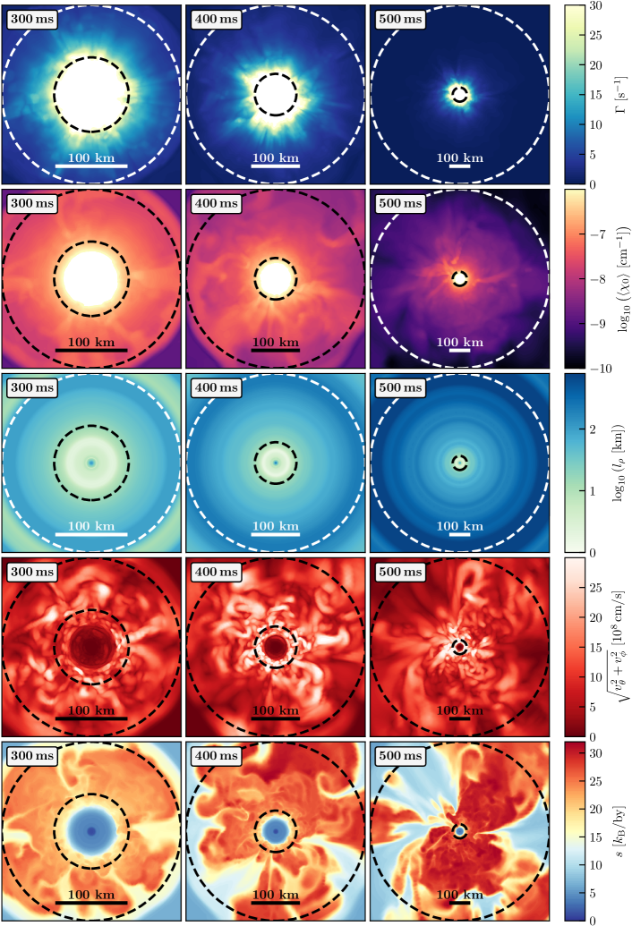
Figure B2: Cross-sectional cuts in the ($x$,$y$)-plane of model s20 with full neutrino transport and uniform $2^{\circ}$ angular resolution at 300 ms, 400 ms, and 500 ms after bounce. From top to bottom, the damping rate associated with the neutrino drag, $\Gamma$ (see Eq. (B70)), the spectrally-averaged neutrino opacity (in the fluid frame) summed over all species, $\langle\chi_{0}\rangle$, the characteristic hydrodynamic length scale, $l_{\rho}$ (see Eq. (B73)), the nonradial velocity, $(v_{\theta}^{2}+v_{\phi}^{2})^{0.5}$, and the entropy per baryon, $s$, are shown. The inner and outer dashed circles indicate the angle-averaged gain radius and the minimum shock radius, respectively.

For the conditions in the gain layer the production of $\nu_{e}$ and $\bar{\nu}_{e}$ plays a subordinated role compared to their absorption. The first summand in Eq. (B66) is therefore negligible. From Eqs. (B68) and (B69) it is clear that in the limit of radially streaming neutrinos at large distances (i.e., $\mu_{\mathrm{min}}\to 1$) the nonradial components vanish and therefore, to first order in $v/c$, radiation drag acts only on the radial velocity component. Nonradial effects depend on Doppler shifts of the neutrino quantities and have dropped out in Eq. (B6), because they are of higher than linear order in $v/c$. During the accretion phase of the stalled supernova shock the spectral shape parameters $\alpha$ are typically between 2 and 3 (Mirizzi et al., 2016; Tamborra et al., 2012). The case of $\alpha=2$ corresponds to a Maxwell-Boltzmann spectrum, $\alpha\approx 2.3$ describes a Fermi-Dirac spectrum with vanishing degeneracy parameter ($\psi=0$), and $\alpha>2.3$ yields pinched spectra with a faster decline beyond the maximum than the Fermi-Dirac distribution.

Table 4: Local evaluation of the neutrino-drag number, Dr, at different radii $R_{\mathrm{ev}}$ for model s20.

						$\mathrm{[10^{-9}\,cm^{-1}]}$
200	76	29	1.19	16.7	24	63.2	52.1	24.7
	78	31	1.19	15.7	25	58.0	48.4	22.9
	$R_{0}$	31	1.19	16.4	24	61.4	50.9	24.1
	avg	30	1.18	16.2	24	59.9	49.8	23.6
300	64	23	1.32	20.5	28	40.7	35.3	14.5
	100	55	1.03	8.1	23	12.7	11.5	4.9
	121	94	0.94	5.4	19	9.4	8.5	3.7
	$R_{0}$	45	1.11	9.5	26	15.0	13.6	5.8
	avg	60	1.07	9.1	20	15.1	13.7	5.8
400	56	19	1.75	30.1	30	46.6	40.4	16.1
	100	48	1.44	8.5	35	10.1	9.2	3.9
	150	101	1.06	3.4	31	4.3	3.9	1.7
	188	215	0.90	1.9	22	2.8	2.6	1.1
	$R_{0}$	69	1.28	5.3	35	6.3	5.8	2.5
	avg	113	1.16	4.8	21	6.2	5.6	2.4
500	50	17	2.34	34.1	41	41.0	36.1	14.1
	100	52	1.55	7.6	39	6.5	6.0	2.5
	150	84	1.35	2.9	55	2.6	2.4	1.0
	200	115	1.25	1.4	79	1.3	1.2	0.5
	250	185	1.15	0.8	82	0.7	0.7	0.3
	300	217	1.03	0.4	118	0.4	0.4	0.2
	350	320	0.96	0.2	123	0.3	0.3	0.1
	400	420	0.89	0.1	142	0.2	0.2	0.1
	450	636	0.82	0.1	125	0.1	0.1	0.1
	500	722	0.77	0.1	165	0.1	0.1	0.1
	$R_{0}$	182	1.09	0.5	112	0.5	0.5	0.2
	avg	438	0.95	0.5	45	0.5	0.5	0.2

B.4 Model-based evaluation

In order to quantify the neutrino-drag effects in numerical simulations, we analyse our 3D model s20 with full neutrino transport and uniform angular resolution of $2^{\circ}$ (see Table 1). Since Prometheus-Vertex contains a Newtonian hydrodynamics solver, we consider —in the spirit of the remark in the footnote in Section B.1— only the third term on the rhs of Eq. (B6). With their ray-by-ray approach to neutrino transport, the simulations provide results compatible with the symmetry assumptions for the neutrino-radiation field considered in Section B.3.

For the quantitative analysis, we apply several simplifications, which ease the evaluation and are acceptable in view of other approximations connected to the ray-by-ray transport, which evolves only the radial components of the neutrino fluxes and assumes the neutrino phase-space distributions to be axially symmetric around the radial direction. First, we focus on the radial term of the neutrino drag, which dominates the nonradial ones, as can be seen by comparing Eq. (B43) with Eq. (B44) and Eq. (B68) with Eq. (B69). Second, we do not transform the radiation quantities, in particular the radiation-pressure tensor, $\mathbf{P}(\epsilon)$, into the laboratory frame. Instead, we evaluate the drag terms with the pressure tensor computed in the comoving frame of the fluid by the transport solver, in line with the available opacities $\chi_{0}$. This simplification is justified because on the one hand the typical fluid velocities in the postshock layer are at most 5–10 % of the speed of light, and on the other hand effects of the transformation between lab frame and comoving frame act in opposite directions in convective downdrafts and outflows and therefore partly compensate each other in the angle-averaged quantities considered here. Third, we use only the nonradial fluid velocities in the postshock layer as a proxy of the turbulent velocities in order to facilitate the direct comparison with the numerical viscosity and Reynolds number along the lines of their evaluation in Sect. 5.

Therefore, using Eq. (B10), we compute the damping rate associated with the neutrino drag according to

$$\Gamma = \frac{|G_{\mathrm{drag}}|}{\rho\,v}=$$ (B70)

$$= \frac{1}{\rho\,c}\sum_{\nu_{i}}\int_{0}^{\infty}\mathrm{d}\epsilon\left[\chi_{0,\nu_{i}}+\epsilon\frac{\partial\chi_{0,\nu_{i}}}{\partial\epsilon}\right]P_{\nu_{i}}(\epsilon)\,,$$

with $P_{\nu_{i}}(\epsilon)$ given by the transport solver as integral of the direction-dependent neutrino intensities according to Eq. (B42). The neutrino-drag number, Dr, can then be calculated with Eq. (B15). To directly compare Dr with the numerical Reynolds numbers, Re, of our simulation, we employ the same definitions for the characteristic turbulent velocity, $v$, and for the length scale of the largest turbulent eddies, $l$, as in Section 5.2.2, namely

$$v^{2}=\frac{1}{4\pi}\int\mathrm{d}\Omega\,(v_{\theta}^{2}+v_{\phi}^{2})\,,$$ (B71)

$$l=R_{\mathrm{sh}}-R_{\mathrm{gain}}\,,$$ (B72)

where $R_{\mathrm{sh}}$ and $R_{\mathrm{gain}}$ are the angle-averaged shock radius and gain radius, respectively. Note that we use a different naming convention here to avoid confusion of the length scale, $l$, with the neutrino luminosity, $L$.

In Table 3 we list the neutrino-drag numbers, averaged over the gain layer of model s20, at different post-bounce times, $t_{\mathrm{pb}}$, as well as the numerical Reynolds numbers, Re, and numerical viscosities, $\nu_{\mathrm{N}}$, obtained with our MKJ method based on the energy dissipation rate (see Section 5.2.2). As in Section 5, all hydrodynamical quantities are measured at radius $R_{0}$ (Eq. (20)) half-way between the average gain radius and the minimum shock radius, $R_{\mathrm{sh,min}}$, and smoothed by performing an average over a radial shell of $R_{0}\pm 5\,\mathrm{km}$ and an additional time average over the interval $t_{\mathrm{pb}}\pm 2.5\,\mathrm{ms}$. The neutrino-drag numbers, Dr, are computed according to Eq. (B15) with the neutrino-damping rate $\Gamma$ from Eq. (B70) and with the same values of $v$ and $l$ as used in the evaluation of the numerical Reynolds numbers. $L_{\nu_{i}}$ are the neutrino luminosities (of species $\nu_{i}=\nu_{e},\bar{\nu}_{e},\nu_{x}$) in the lab frame and $\kappa_{\nu_{i}}\equiv\langle\chi_{0}\rangle_{\nu_{i}}$ the spectrally-averaged neutrino opacities in the comoving frame of the stellar fluid. The neutrino-related quantities, $\Gamma$, $L_{\nu_{i}}$, and $\kappa_{\nu_{i}}$, are spatially averaged over a radial shell extending from $R_{\mathrm{gain}}+10\,\mathrm{km}$ to $R_{\mathrm{sh,min}}-10\,\mathrm{km}$ and time-averaged over $t_{\mathrm{pb}}\pm 2.5\,\mathrm{ms}$.

Since the matter density $\rho$, the neutrino opacities, and the neutrino radiation quantities, all of which enter the computation of the damping rate $\Gamma$ (see Eq. (B70)) and drag number Dr (Eq. (B15)), decline with increasing radius, we also investigate the radial dependence of the neutrino drag in the gain layer. Thus we intend to test ambiguities in the determination of the neutrino-drag effects in terms of the characteristic parameter Dr. Figure B2 displays some of the relevant quantities in a cross-sectional plane at different post-bounce times to demonstrate their spatial variations in connection with the convective vortex flows. In order to perform a radius-dependent analysis, we define a characteristic local hydrodynamic length scale, constrained by the width of the gain layer, as

$$l_{\rho}=\min\left(\frac{\bar{\rho}}{\left|\mathrm{d}\bar{\rho}/\mathrm{d}r\right|}\,,\,R_{\mathrm{sh}}-R_{\mathrm{gain}}\right),$$ (B73)

where $\bar{\rho}$ is the angle-averaged matter density. Moreover, we use local, shell-averaged values of the nonradial (turbulent) velocity, $v$, and of the damping rate, $\Gamma$ (Eq. (B70)), in Eq. (B15) for estimating local values of Dr. The corresponding results are listed in Table 4, where all local quantities are time-averaged over 5 ms and radially averaged over shells of 10 km thickness around the locations of evaluation, $R_{\mathrm{ev}}$.

The data for the neutrino-drag number Dr in Tables 3 and 4 are consistent with our order-of-magnitude estimate of Eq. (B16). Typical values are several 10 up to more than 100 in the gain layer. Naturally, the drag numbers become particularly small when computed with the radial width of the entire gain layer in Table 3, but also the local values of Table 4 are only a factor of $\sim$2 bigger, except at large radii at 500 ms, where the neutrino opacities and neutrino pressure $P(r)$, and correspondingly the neutrino-damping rate, become small. A comparison of the numerical Reynolds numbers, Re, and the neutrino-drag numbers, Dr, in Table 3 confirms that on the scale of large and largest turbulent eddies in our 2^∘ simulation of model s20, the neutrino drag clearly dominates the effects of numerical viscosity. Only on scales smaller than $l\leq\sqrt{\nu_{\mathrm{N}}/\Gamma}$ does damping by numerical viscosity become compatible with the influence of the neutrino drag on fluid motions. This corresponds to vortex flows of less than 10–20 km diameter near the gain radius ($R_{\mathrm{gain}}\sim 50$–70 km) and of less than 50–60 km near the shock at a radius of about 200 km.

Neutrino-damping rates of $\sim 5$–10 s^-1 in the gain layer suggest typical damping timescales of large-scale fluid motions on the order of 100–200 ms. Such timescales may be short enough to slightly delay or hamper the onset of postshock convection. A quantitative assessment of such effects and their potential consequences for the onset of an explosion would require a comparison with the model-specific growth timescales of convection or SASI in the postshock layer. However, with large-scale pre-collapse perturbations in the convective silicon- and oxygen-burning shells of the progenitor (e.g., Couch & Ott, 2013; Müller & Janka, 2015; Couch et al., 2015; Müller et al., 2016; Yoshida et al., 2019; Yadav et al., 2019), the driving force for the growth of instabilities (e.g., Müller et al., 2017; Kazeroni & Abdikamalov, 2019) should be sufficiently strong to render neutrino drag a subdominant effect.

Our conclusions should not be severely affected by the simplifications made in our analysis as mentioned at the beginning of this section. Although considering nonradial velocities might moderately underestimate the neutrino-drag number (because the radial velocities may be somewhat higher), a rigorous evaluation of the neutrino drag requires to sum up all components of the vector-matrix product in the third term on the rhs of Eq. (B6) with nonvanishing offdiagonal matrix components. This would increase the neutrino-damping rate and reduce the drag number, thus countersteering the velocity dependence. However, in order to account for the effects of the neutrino drag fully quantitatively, one needs a transport treatment that does not only include all velocity-dependent terms at least up to first order in $v/c$, but in addition it also requires a scheme that reaches beyond the ray-by-ray approximation and therefore provides reliable values for the offdiagonal elements of the neutrino pressure tensor, too. All of these terms must be included with proper frame dependences in the momentum equation of the stellar plasma as discussed in Section B.1.