Causal comparative effectiveness analysis of dynamic continuous-time treatment initiation rules with sparsely measured outcomes and death

Abstract

Evidence supporting the current World Health Organization recommendations of early antiretroviral therapy (ART) initiation for adolescents is inconclusive. We leverage a large observational data and compare, in terms of mortality and CD4 cell count, the dynamic treatment initiation rules for HIV-infected adolescents. Our approaches extend the marginal structural model for estimating outcome distributions under dynamic treatment regimes (DTR), developed in Robins et al. (2008), to allow the causal comparisons of both specific regimes and regimes along a continuum. Furthermore, we propose strategies to address three challenges posed by the complex data set: continuous-time measurement of the treatment initiation process; sparse measurement of longitudinal outcomes of interest, leading to incomplete data; and censoring due to dropout and death. We derive a weighting strategy for continuous time treatment initiation; use imputation to deal with missingness caused by sparse measurements and dropout; and define a composite outcome that incorporates both death and CD4 count as a basis for comparing treatment regimes. Our analysis suggests that immediate ART initiation leads to lower mortality and higher median values of the composite outcome, relative to other initiation rules.

1 Introduction

1.1 Dynamic treatment regimes and treatment of pediatric HIV infection

HIV/AIDS continues to be one of the leading causes of burdensome disease in adolescents (10–19 years old). Globally, an estimated 2.1 million adolescents were living with HIV in 2013, with most living in sub-Saharan Africa (WHO, 2015). Current World Health Organization (WHO) treatment recommendations for adolescents call for initiation of antiretroviral therapy (ART) upon diagnosis with HIV (WHO, 2015). Previously, and particularly for resource-limited settings (RLS), WHO recommendations called for delaying treatment until a clinical benchmark signaling disease progression was reached. For example, the 2013 guidelines recommended initiating ART when CD4 cell count – a marker of immune system function – fell below 500.

For investigating the effectiveness of ART initiation rules, adolescents are a subpopulation of particular interest, particularly because of issues related to drug adherence (Mark et al., 2017). For adolescents, early initiation of ART can potentially increase the risk of poor adherence, leading to development of drug resistance, while initiating too late increases mortality and morbidity associated with HIV. Evidence from both clinical trials (Luzuriaga et al., 2004; Violari et al., 2008) and observational studies (Berk et al., 2005; Schomaker et al., 2017) supports the immediate ART initiation rule recommended by the WHO for children under 10 years of age. Conclusive evidence is lacking for adolescents. The 2015 WHO guidelines did not identify any study investigating the clinical outcomes of adolescent-specific treatment initiation strategies (WHO, 2015). A recent large-scale study (Schomaker et al., 2017) of HIV-infected children (1–9 years) and adolescents (10–16 years) found mortality benefit associated with immediate ART initiation among children, but inconclusive results for the adolescents, and recommended further study of this group. Evaluating ART initiation rules specific to adolescents therefore remains important.

Prior to 2015, WHO guidelines for treatment initiation were expressed in the form of a dynamic treatment regime (DTR), formulated as “initiate when a specific marker crosses threshold value $q$”. In a DTR, the decision to initiate treatment for an individual can depend on evolving treatment, covariate, and marker history (Chakraborty and Murphy, 2014).

In this paper, we use observational data on 1962 HIV-infected adolescents, collected as part of the East Africa IeDEA Consortium (Egger et al., 2012) to compare the effectiveness of CD4-based DTR, with emphasis on comparisons to the strategy of immediate treatment initiation. Our approach is to emulate a clinical trial in which individuals are randomized at baseline and then followed for for a fixed amount of time, at which point mortality status and, for those remaining alive, CD4 cell count are ascertained. Hence the utility function for our comparison involves both mortality and CD4 count among survivors.

In addition to the usual complication of time-varying confounding caused by treatment not being randomly allocated, the structure of the dataset poses three specific challenges that we address here. First, unlike with many published analyses comparing dynamic treatment regimes, treatment initiation is measured in continuous time; second, the outcome of interest, CD4, is measured infrequently and at irregularly spaced time intervals, leading to incomplete data at the target measurement time; third, some individuals may not complete follow up, leading to censoring of both death time and CD4 count.

We use inverse probability weighting (IPW) to handle confounding, and imputation to address missingness due to sparse measurement and censoring. To deal with continuous-time measurement of treatment initiation, we derive continuous-time versions of the relevant probability weights. To deal with missingness, we rely on imputations from a model of the joint distribution of CD4 count and mortality fitted to the observed data. We take a two-step approach: first, the joint model is fitted to the observed data and used to generate (multiple) imputations of missing CD4 and mortality outcomes; second, we apply IPW to the filled-in datasets to generate causal comparisons between different DTR.

1.2 Comparing dynamic treatment regimes using observational data

Randomized controlled trials can be used to evaluate a DTR of the form described above. (see Violari et al., 2008 for example). Observational data afford large sample sizes and rich information on treatment decisions, but the lack of randomization motivates the need to use specialized methods for drawing valid causal comparisons between regimes. Statistical methods for drawing causal inferences about DTR from observational data include the g-computation algorithm (Robins, 1986), inverse probability weighted estimation of marginal structural models (Robins et al., 2008), and g-estimation of structural nested models (Moodie et al., 2007); see Daniel et al. (2013) for a comprehensive review and comparison.

The g-computation formula was first introduced by Robins (1986) and has been used to deal with time-dependent confounding when estimating the causal effect of a time-varying treatment. The unobserved potential outcomes and intermediate outcomes that would have been observed under different hypothetical treatments are predicted from models for potential outcomes and models for time-varying confounders. The predicted potential outcomes under different hypothetical DTR assignments are then contrasted for causal effect estimates. As the number of longitudinal time points increase, the method more heavily leverages parametric modeling assumptions used for extrapolation of covariates and outcomes, increasing the reliance on these assumptions and introducing potential for bias from model mis-specification.

The IPW approach re-weights each individual inversely by the probability of following specific regimes so that, in the weighted population, treatment can be regarded as randomly allocated to these regimes. Time-varying weights are required for handling time-dependent confounding. This involves specifying a model for treatment trajectory over longitudinal follow-up that can include time-dependent covariates. The IPW approach does not require models for the distribution of outcomes and covariates, which in principle makes it less susceptible to model misspecification than the g-computation formula. The method can however generate unstable parameter estimates if there are extreme weights, raising the possibility of finite-sample bias, which can often be alleviated by using stabilized weights or truncation (Cole and Hernán, 2008; Cain et al., 2010).

1.3 IeDEA data

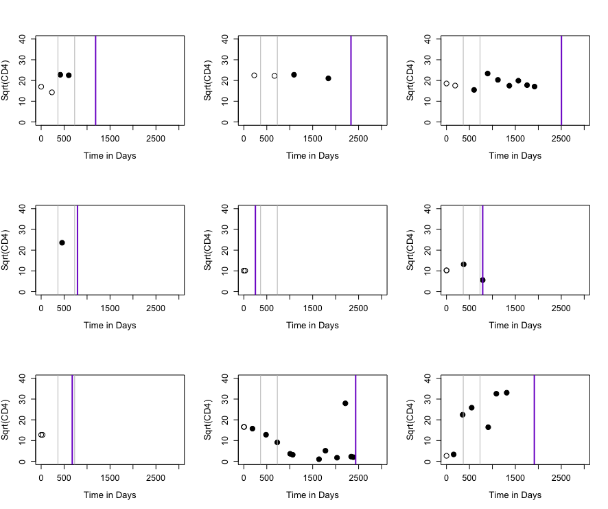
Figure 1: CD4 and ART initiation status during follow up for 9 randomly selected individuals. Empty circles indicate no ART and filled circles represent on ART. Two gray lines denote one year and two years post diagnosis. Purple line corresponds to end of follow up.

The IeDEA consortium, established in 2005, collects clinical and demographic data on HIV-infected individuals from seven global regions, four of which are in Africa. Data from African regions derive from 183 clinics providing ART (Egger et al., 2012). Our analysis makes use of clinical encounter data, drawn from the East Africa region, on 1962 HIV-infected and ART naive adolescents who were diagnosed with HIV between February 20, 2002 and November 19, 2012. The dataset contains individual-level information at diagnosis on the following variables: age, gender, clinic site, CDC class (a 4-level ordinal diagnostic indicator of HIV severity), CD4 count, weight-for-age Z scores (WAZ) and height-for-age Z scores (HAZ). The dataset also includes longitudinal information on ART initiation status, death, CD4 count, WAZ and HAZ. These data were generated before the 2015 WHO guidelines that recommend immediate ART initiation, which yields significant variability in ART initiation patterns observed in our data.  The follow-up visits vary considerably from patient to patient, resulting in irregularly and sparsely measured CD4 cell count (1.71, 1.32, 1.10 per person per year within one, two and three years of diagnosis) and various ART initiation patterns (Figure 1). Kaplan-Meier estimates of mortality one-, two- and three-years post diagnosis are 3.3%, 4.5% and 5.6% respectively.

Our goal is to compare CD4 cell count and mortality rate at one and two years post enrollment under dynamic regimes defined in terms of initiating treatment at specific CD4 threshold values. In the next section we define the randomized trial our analysis is designed to emulate, and the outcome measure (utility) used for the comparisons.

The remainder of the paper is organized as follows: Section 2 describes notation and the statistical problem. Section 3 delineates the approaches to estimating and comparing dynamic continuous-time treatment initiation rules with sparsely measured outcomes and death. Section 4 presents results from our analysis of IeDEA data and highlights new insights relative to previous studies. Section 5 provides a summary and directions for future research.

2 Notation and dynamic regimes

2.1 Randomized trial being emulated to compare dynamic regimes

Ideally, causal comparisons of dynamic regimes should be based on a hypothetical randomized trial (Hernán et al., 2006). In our setting, the trial we are emulating would randomize individuals at time $t=0$ to regimes in a set $\mathscr{Q}=\{0,200,210,220,\ldots,490,500,\infty\}$, where $q=0$ corresponds to ‘never treat’ and $q=\infty$ denotes ‘treat immediately’, and other regimes correspond to initiating treatment when CD4 falls below $q$. Each individual would be followed to a specific time point $t^{*}$, at which point survival status would be ascertained and, for those surviving to $t^{*}$, CD4 would be measured. For those who discontinue follow up prior to $t^{*}$, we assume treatment status (on or off) at the time of discontinuation would still apply at $t^{*}$.

For each individual, let $\{D_{q}:q\in\mathscr{Q}\}$ represent the set of potential outcomes, one for each regime, indicating death at $t^{*}$, such that $D_{q}=1$ if dead and $D_{q}=0$ if alive. Similarly define $\{Y_{q}:q\in\mathscr{Q}\}$ to be the set of potential CD4 counts for an individual who survives to $t^{*}$. Now define, for $q\in\mathscr{Q}$, the composite outcome $X_{q}=(1-D_{q})Y_{q}$, with $X_{q}=0$ for those who die prior to $t^{*}$ and $X_{q}=Y_{q}>0$ for those who survive. We use both mortality rate $P(D_{q}=1)=P(X_{q}=0)$ and quantiles of $X_{q}$ as a basis for comparing treatments. The cumulative distribution function (CDF) of $X_{q}$ is a useful measure of treatment utility because it has point mass at zero corresponding to the mortality rate, and thereby reflects information about both mortality and CD4 cell count among survivors; e.g., $P(X_{q}>0)$ is the survival fraction and $P(X_{q}>x)$, for $x>0$, is proportion of individuals who survive to $t^{*}$ and have CD4 count greater than $x$.

2.2 Defining dynamic treatment regime

Let $\{Z(t):t\geq 0\}$, where $Z(t)>0$, represent CD4 cell count, which is defined for all $t$ but measured only at discrete time points for each individual (see below). Let $T$ denote survival time, with $\{N^{T}(t):t>0\}$ its associated zero-one counting process. Each individual has a $p\times 1$ covariate process $\{L(t):t\geq 0\}$, some elements of which may be time varying. The time-varying covariates may be recorded at times other than those where $Z$ is recorded. Finally let $A$ denote the time of treatment initiation, with associated counting process $\{N^{A}(t):t\geq 0\}$ and intensity function $\lambda^{A}(t)$. Adopting a convention in the DTR literature (Robins et al., 2008), we assume the decision to initiate ART at $t$ is made after observing the covariates and CD4 cell count; that is, for a given $t$, $N^{A}(t)$ occurs after $Z(t)$ and $L(t)$. Finally let $C$ be a censoring (dropout) time, with associated counting process $N^{C}(t)$.

At a fixed time $t$, let $H(t)=\{Z(t),N^{T}(t),L(t),N^{A}(t),N^{C}(t)\}$ represent the most recent values of each process. We use overbar notation to denote the history of a process, so that (e.g.) $\overline{L}(t)=\{L(s):0\leq s\leq t\}$ is the history of $L(t)$ up to $t$. All individuals are observed at baseline and then at a discrete number of time points whose number, frequency and spacing may vary. Hence the observed-data process for individual $i$ $(=1,\ldots,n)$ is denoted by $\overline{H}_{i}(t_{iK_{i}})=\{H_{i}(t):t=0,t_{i1},t_{i2},\ldots,t_{iK_{i}}\}$.

2.3 Mapping observed treatment to dynamic treatment regime

The dynamic treatment regime ‘initiate treatment when $Z(t_{j})$ falls below threshold $q$’ (where $t_{j}$ is time at the $j$th visit) is a deterministic function $r_{q}(\overline{H}(t_{j}))$ that depends on observed values of $\overline{Z}(t_{j})$ and treatment history $\overline{N}^{A}(t_{j})$; for brevity we suppress subscript $j$ and write $r_{q}(t)$, which applies to each individual’s actual visit times. As some patients have missing baseline CD4, let $R^{Z}(t)$ be a binary indicator with $R^{Z}(t)=1$ denoting that CD4 has not been observed by time $t$. At $t=0$, the rule is $r_{q}(0)=I\{R^{Z}(0)=1\text{ or }Z(0)<q\}$, indicating immediate initiation regardless of $Z(0)$ or treat if $Z(0)$ is below $q$. For $t>0$, we define $Z_{\text{min}}(t)=\min_{j:0\leq t_{j}<t}Z(t_{j})$ to be the lowest previously recorded value of $Z$ prior to $t$. Then,

$$r_{q}(t) = \left\{\begin{array}[]{cl}0&\text{ if }\{N^{A}(t^{-})=0\text{ and }Z_{\min}(t)\geq q\text{ and }Z(t)\geq q\}\text{ or }R^{Z}(t)=1,\\ 1&\text{ if }N^{A}(t^{-})=0\text{ and }Z_{\min}(t)\geq q\text{ and }Z(t)<q,\\ 1&\text{ if }N^{A}(t^{-})=1.\end{array}\right.$$

In words, the first line of the rule says not to treat if an individual has not yet initiated treatment and $Z(t)$ has not fallen below $q$ or has not been observed; the second line says to treat if time $t$ represents the first time $Z(t)$ has fallen below $q$; the third line says to keep treating once ART has been initiated.

In addition to the observed data process, we define a regime-specific compliance process $\{\Delta_{q}(t):t\geq 0\}$ where $\Delta_{q}(t)=1$ if regime $q$ is being followed at time $t$ and $\Delta_{q}=0$ otherwise. Written in terms of $\overline{H}(t)$ and $r_{q}(t)$, we have $\Delta_{q}(t)=N^{A}(t)r_{q}(t)+\{1-N^{A}(t)\}\{1-r_{q}(t)\}.$ Hence if an individual’s actual treatment status at time $t$ agrees with the DTR $q$, then this individual is compliant with regime $q$ at time $t$. Thus for each individual and for each $q\in\mathscr{Q}$, we observe, in addition to $\overline{H}(t)$, a regime compliance process $\left\{\Delta_{qi}(t):t=0,t_{i1},\ldots,t_{iK_{i}}\right\}$.

2.4 Missing outcomes due to sparse measurement times and censoring

For those who remain alive at $t^{*}$, the observed $X_{i}$ corresponds to $Z_{i}(t^{*})$. When measurement of $Z_{i}(t)$ is sparse and irregular, $Z_{i}(t^{*})$ will not be directly observed unless $t_{ik}=t^{*}$ for some $k\in\{1,\ldots,K_{i}\}$. In settings like this, it is common to define the observed outcome as the value of $Z_{i}(t)$ closest to $t^{*}$ and falling within a pre-specified interval $[t_{a},t_{b}]$ containing $t^{*}$. Specifically, $X_{i}$ is the value of $Z(t_{ik})$ such that $t_{ik}\in[t_{a},t_{b}]$ and $|t_{ik}-t^{*}|$ is minimized over $k$. Even using this definition, the interval $[t_{a},t_{b}]$ still may not contain any of the measurement times for some individuals; hence $X_{i}$ can be missing even for those who remain in follow up at $t^{*}$. The other cause of missingness in $X_{i}$ is dropout, which occurs when $t_{iK_{i}}<t_{a}$.

For both of these situations, we rely on multiple imputation based on a model for the joint distribution of the CD4 process $Z(t)$ and the mortality process $N^{T}(t)$. The general strategy is as follows: first, we specify and fit a model for the joint distribution $[Z(t),N^{T}(t){\,|\,}\overline{H}(t)]$ of CD4 and mortality, conditional on observed history. For those who are known to be alive but do not have a CD4 measurement within the pre-specified interval $[t_{a},t_{b}]$, we impute $\widetilde{X}_{i}\sim[{Z}(t^{*}){\,|\,}\overline{H}_{i}(t^{*})]$ from the fitted CD4 submodel. For those who are missing $X_{i}$ because of right censoring, we proceed as follows: (i) calculate $P\{N^{T}(t^{*})=1{\,|\,}\overline{H}_{i}(t_{iK_{i}})\}$ from the fitted survival submodel, and impute $\widetilde{D}_{i}$ from a Bernoulli distribution having this probability; (ii) for those with $\widetilde{D}_{i}=0$, impute $\widetilde{X}_{i}\sim[{Z}(t^{*}){\,|\,}\overline{H}_{i}(t^{*})]$ from the fitted CD4 submodel; (iii) for those with $\widetilde{D}_{i}=1$, set $\widetilde{X}_{i}=0$. Further details are given in Section 3.5.

3 Estimating and comparing effectiveness of dynamic regimes

3.1 Assumptions needed for inference about dynamic regimes

We are interested in parameters or functionals of the potential outcomes distribution $F_{X_{q}}(x)=P(X_{q}\leq x)$. Specific quantities of interest are the mortality rate $\theta_{q1}=P(X_{q}=0)=F_{X_{q}}(0)$, the median of the distribution of the composite outcome $\theta_{q2}=F_{X_{q}}^{-1}({\textstyle\frac{1}{2}})$, and the mean CD4 count among survivors $\theta_{q3}=E(X_{q}{\,|\,}X_{q}>0)$. We first consider inference in the case where there is no missingness in the observable outcomes $X_{i}$. Estimates for each of these quantities can be obtained using weighted estimating equations under specific assumptions.

A1. Consistency assumption. To connect observed data to potential outcomes, we use the consistency relation $X_{i}=X_{qi}$ when $\Delta_{qi}(t^{*})=1$, for all $q\in\mathscr{Q}$, which implies that the observed outcome $X_{i}$ corresponds to the potential outcome $X_{qi}$ when individual $i$ actually follows regime $q$. Note that an individual can potentially follow more than one regime at any given time.

A2. Exchangeability assumption. In observational studies, individuals are not randomly assigned to follow regimes. Decisions on when to start ART are often made by based on guidelines and observable patient characteristics. We make the following exchangeability assumption, also known as sequential randomization of treatment: $\lambda^{A}(t{\,|\,}\overline{H}(t),T>t,X_{q})=\lambda^{A}(t{\,|\,}\overline{H}(t),T>t)$, for $t<t^{*}$. This assumption states that initiation of treatment at $t$ among those who are still alive is conditionally independent of the potential outcomes $X_{q}$ conditional on observed history $\overline{H}(t)$.

A3. Positivity assumption. Finally we assume that at any given time $t$, there is positive probability of initiating treatment, among those who have not yet initiated, for all configurations $\overline{H}(t)$ (Robins et al., 2008): $P\left\{\lambda^{A}(t{\,|\,}\overline{H}(t),T>t)>0\right\}=1$. This implicitly assumes a positive probability of visiting clinic in the interval $[t,t^{*}]$, conditional on $\overline{H}(t)$.

3.2 Weighted estimating equations for comparing specific regimes

For illustration, consider estimating the mortality rate $\theta_{q1}=P(X_{q}=0)$. If individuals are randomized to specific regimes, a consistent estimator of the death rate is the sample proportion among those who follow regime $q$; i.e., $\widehat{\theta}_{q1}=\sum_{i}\Delta_{qi}(t^{*})I(X_{i}=0)\left/\sum_{i}\Delta_{qi}(t^{*})\right.$. This estimator is the solution to $\sum_{i}\Delta_{qi}(t^{*})\{I(X_{i}=0)-\theta_{q1}\}=0$, which is an unbiased estimating equation when $\theta_{q1}=\theta_{q1}^{*}$ is the true value of $\theta_{q1}$. We can similarly construct unbiased estimating equations for other quantities of interest. For example, under randomization, a consistent estimator of the median of $X_{q}$ is the solution to $\sum_{i}\Delta_{qi}(t^{*})\left\{I(X_{i}\leq\theta_{q2})-{\textstyle\frac{1}{2}}\right\}=0$.

For observational data, relying on the assumptions of consistency, positivity and exchangeability, we can obtain consistent estimates of quantities of interest using weighted estimating equations. Returning to mortality rate, a consistent estimator of $\theta_{q1}$ can be obtained as the solution to the weighted estimating equation $\sum_{i=1}^{n}\Delta_{qi}(t^{*})W_{qi}\left\{I(X_{i}=0)-\theta_{q1}\right\}=0$, where $W_{qi}=1/P\{\Delta_{q}(t^{*})=1{\,|\,}\overline{H}_{i}(t^{*})\}$ is the inverse probability of following regime $q$ through time $t^{*}$ (Robins et al., 2008; Cain et al., 2010; Shen et al., 2017).

In practice the weights $W_{qi}$ must be estimated from data; some of the estimated weights can be large, leading to estimators with high variability (Cain et al., 2010). This problem can be ameliorated to some degree by using stabilized weights of the form

$$W^{s}_{qi} = \frac{P\left\{\Delta_{q}(t^{*})=1\right\}}{P\left\{\Delta_{q}(t^{*})=1{\,|\,}\overline{H}_{i}(t^{*})\right\}}.$$ (2)

In this case, the numerator of the weight function needs to be calculated directly from the regime indicator processes. Specifically, for each regime $q$, define a 0-1 counting process $N^{q}(t)=1-\Delta_{q}(t)$ that jumps when regime $q$ is no longer being followed, and let $\Lambda^{q}(t)$ denote its associated cumulative hazard function. Then $S^{q}(t)=P\{N^{q}(t)=0\}=P\{\Delta_{q}(t)=1\}$; hence (an estimate of) $S^{q}(t^{*})=\exp\{-\Lambda^{q}(t^{*})\}$ can be used as the numerator weight.

3.3 Comparing regimes along a continuum

We can examine the effect of DTR $q$ on $X_{q}$ at a higher resolution along a continuum such as $\mathscr{Q}=\{200,210,\ldots,500\}$ (we use integers for $\mathscr{Q}$, but theoretically it can include continuous values). When the number of regimes to be compared is large, it is highly possible that not every regime is followed by a sufficiently large number of individuals, and sampling variability associated with the regime effect estimated using the procedure for discrete regimes may be large (Hernán et al., 2006). A statistically more efficient approach is to formulate a causal model that captures the smoothed effect of $q$ on a parameter of interest; we illustrate using the median $\theta_{q2}=F^{-1}_{X_{q}}({\textstyle\frac{1}{2}})$.

Let $q_{l}$ and $q_{u}$ denote the lower and upper bound of the regime continuum. Assume $F^{-1}_{X_{q}}(\tau)$, where $\tau$ is a fixed quantile, follows a structural model

$$F^{-1}_{X_{q}}(\tau) = \alpha_{0}I(q=\infty)+\alpha_{1}I(q=0)+I(q\in[q_{l},q_{u}])d(q),$$ (3)

where $d(\cdot)$ is an unspecified function with smoothness constraints. In our application, we use natural cubic splines constructed from piecewise third-order polynomials that pass through a set of control points, or knots, placed at quantiles of $q$. This allows $d(q)$ to flexibly capture the effect of $q$ along the continuum and enables separate estimation of the discrete regimes $q=\infty$ and $q=0$. Parameterizing our model in terms of the basis functions of a natural cubic spline with $J$ knots (Hastie et al., 2009) yields $F^{-1}_{X_{q}}(\tau)=\alpha^{\top}V(q)$, where

$$V(q)_{(J+2)\times 1}=[I(q=\infty),\;I(q=0),\;I(q\in[q_{l},q_{u}])d^{\dagger}(q)^{\top}]^{\top}$$

and $d^{\dagger}(q)=[d^{\dagger}_{1}(q),\cdots,d^{\dagger}_{J}(q)]^{\top}$ are the $J$ basis functions of $d(q)$. The parameter $\alpha$ is a vector of $J+2$ coefficients for $I(q=\infty)$, $I(q=0)$ and the basis functions $d^{\dagger}(q)$. The causal effect of regime $q$ on the potential outcome $X_{q}$ is therefore encoded in the parameter $\alpha$. A consistent estimator of $\alpha$ can be obtained by solving the estimating equation (Leng and Zhang, 2014):

$$\sum_{i}\Delta_{qi}(t)W^{s}_{qi}V_{i}(q)\left[I\{X_{i}-V_{i}^{\top}(q)\alpha>0\}-\tau\right] = 0.$$

Setting $\tau=0.5$ estimates the causal effect of $q$ on the median of $X_{q}$.

3.4 Derivation and estimation of continuous time weights

3.4.1 Assuming no dropout or death prior to $t^{*}$

The denominator of $W^{s}_{qi}$ in equation (2) is the probability of individual $i$ following regime $q$ through $t^{*}$, conditional on observed history $H_{i}(t^{*})$. As described in Robins et al. (2008); Cain et al. (2010) and Shen et al. (2017), for discrete-time settings where the measurement times are common across individuals, this probability corresponds to the cumulative product of conditional probabilities of treatment indicators over a set of time intervals $0=t_{0}<t_{2}<\cdots<t_{K}=t^{*}$. Specifically,

$$P\left\{\Delta_{qi}(t^{*})=1\;\left|\;\overline{H}_{i}(t^{*})\right\}\right. = \prod_{k=0}^{K}P\left(\Delta_{qi}(t_{k})=1\;\left|\;\overline{H}_{i}(t_{k})\right)\right.$$ (4)

$$= \prod_{k=0}^{K}P\left[\left\{N^{A}_{i}(t_{k})r_{qi}(t_{k})+(1-N^{A}_{i}(t_{k}))(1-r_{qi}(t_{k}))\right\}=1\,\left|\,\overline{H}_{i}(t_{k})\right]\right.$$

$$= \prod_{k=0}^{K}\left\{P\left(N^{A}_{i}(t_{k})=1\,\left|\,\overline{H}_{i}(t_{k})\right)I\left(r_{qi}(t_{k})=1\right)\right.\right.$$

$$\hskip 36.135pt+\left.P\left(N^{A}_{i}(t_{k})=0\,\left|\,\overline{H}_{i}(t_{k})\right)I\left(r_{qi}(t_{k})=0\right)\right\}\right..$$

This establishes the connection between regime compliance and treatment history. Equation (4) represents the treatment history among those with $\Delta_{qi}(t^{*})=1$; therefore, to compute the probability of regime compliance for those with $\Delta_{qi}(t^{*})=1$, we just need to model their observed treatment initiation process, as described in equation (5) below.

This observation allows us to generalize the weights for the discrete time setting to the continuous time process. Let $dN_{i}^{A}(t)$ be the increment of $N_{i}^{A}$ over the small time interval $[t,t+dt)$. Note that conditional on $\overline{H}(t)$, the occurrence of treatment initiation for individual $i$ in $[t,t+dt)$ is a Bernoulli trial with outcomes $dN_{i}^{A}(t)=1$ and $dN_{i}^{A}(t)=0$. Equation (4) can therefore be written

$$\prod_{k=0}^{K}P\left(dN_{i}^{A}(t)=1{\,|\,}\overline{H}_{i}(t)\right)^{dN_{i}(t)}P\left(dN_{i}^{A}(t)=0{\,|\,}\overline{H}_{i}(t)\right)^{1-dN_{i}(t)},$$ (5)

which takes the form of the individual partial likelihood for the counting process $\{N_{i}^{A}(t):0\leq t\leq t^{*}\}$. When the number of time intervals between $t_{0}$ and $t_{K}$ increases, $dt$ becomes smaller, and the finite product in (5) will approach a product-integral (Aalen et al., 2008)

$$\Prodi_{0\leq t\leq t^{*}}\left\{\lambda^{A}(t{\,|\,}\overline{H}_{i}(t))dt\right\}^{dN^{A}_{i}(t)}\left\{1-\lambda^{A}(t{\,|\,}\overline{H}_{i}(t))dt\right\}^{1-dN^{A}_{i}(t)}\hskip 144.54pt$$ (6)

$$=\left[\prod_{0\leq t\leq t^{*}}\left\{\lambda^{A}(t{\,|\,}\overline{H}_{i}(t))\right\}^{\Delta N^{A}_{i}(t)}\right]\exp\left\{-\int_{0}^{t^{*}}\lambda^{A}(t{\,|\,}\overline{H}_{i}(t))dt\right\},\hskip 72.26999pt$$ (7)

where $\Delta N^{A}_{i}(t)=N^{A}_{i}(t)-N^{A}_{i}(t^{-})$. The product integral of the first part in (6) is the finite product over the jump times of the counting process, hence the first factor in (7). The second factor in (7) follows from properties of the product-integral of an absolutely continuous function (Aalen et al. 2008, Appendix A.1).

The individual counting process $\{N_{i}^{A}(t),0\leq t\leq t^{*}\}$ will have at most one jump (at $A_{i}$), and in our case patients stay on ART once it is initiated. Hence the product integral only needs to be evaluated up to the ART initiation time. Equation (7) therefore reduces to

$$P\left\{\Delta_{qi}(t^{*})=1{\,|\,}\overline{H}_{i}(t^{*})\right\} = \lambda^{A}(A_{i}{\,|\,}\overline{H}(A_{i}))S^{A}(A_{i}{\,|\,}\overline{H}_{i}(A_{i}))N_{i}(t^{*})+S^{A}(t^{*}{\,|\,}\overline{H}_{i}(t^{*}))\{1-N_{i}(t^{*})\}$$ (8)

$$= f^{A}(A_{i}{\,|\,}\overline{H}_{i}(A_{i}))N^{A}_{i}(t^{*})+S^{A}(t^{*}{\,|\,}\overline{H}_{i}(t^{*}))\{1-N^{A}_{i}(t^{*})\},$$

where $S^{A}(t{\,|\,}\overline{H}(t))=\exp\{-\Lambda^{A}(t{\,|\,}\overline{H}(t))\}$ is the survivor function associated with the ART initiation process.

For an alternate derivation of the continuous time weights, see Johnson and Tsiatis (2005), who use a Radon-Nikodym derivative of one integrated intensity process (under randomized treatment allocation) with respect to another (for the observational study), and arrive at the same weighting scheme as ours. Simulation studies by Hu et al. (2018) demonstrate consistency and stability of weighted estimators using continuous-time weights in empirical settings when assumptions A1-A3 hold and the weight model is correctly specified.

Components of the denominator weights are estimated from a fitted hazard model for treatment initiation. Specifically we assume $\lambda^{A}(t{\,|\,}\overline{H}(t))$ follows a Cox proportional hazards model $\lambda^{A}(t{\,|\,}\overline{H}(t))=\lambda_{0}^{A}(t)u(\overline{H}(t);\phi)$, where $u$ is a strictly positive function capturing the effect of covariates and $\phi$ is a finite-dimensional parameter vector. Details of the model specification used in our application are given in Section 4. The parameter $\phi$ is estimated using maximum partial likelihood estimation, and the baseline hazard function $\lambda^{A}_{0}(t)$ is estimated using the Nelson-Aalen estimator. The functions $f^{A}$ and $S^{A}$ are estimated via

$$\widehat{S}^{A}(t{\,|\,}\overline{H}(t)) = \exp\left\{-\int_{0}^{t}u(\overline{H}(s);\widehat{\phi})\;d\widehat{\Lambda}^{A}_{0}(s)\right\},$$ (9)

$$\widehat{f}^{A}(t{\,|\,}\overline{H}(t)) = d\widehat{\Lambda}^{A}(t{\,|\,}\overline{H}(t))\;\widehat{S}^{A}(t{\,|\,}\overline{H}(t)).$$ (10)

To estimate the stabilizing numerator weight $P\left\{\Delta_{q}(t^{*})=1\right\}$, we use the $q$-specific survivor function associated with the counting process $N^{q}(t)$, estimated using the Nelson-Aalen estimator $\widehat{S}^{q}(t^{*})=\exp\{-\widehat{\Lambda}^{q}(t^{*})\}$.

3.4.2 Considering dropout or death prior to $t^{*}$

In the IeDEA data, some participants drop out prior to $t^{*}$, which requires modifications to the weight specification. We make an additional assumption:

A4. Conditional constancy assumption. Once lost to follow up at $C_{i}<t^{*}$, treatment and regime status remain constant; i.e., $N^{A}(t)=N^{A}(C_{i})$ and $\Delta_{qi}(t)=\Delta_{qi}(C_{i})$ for all $t\in[C_{i},t^{*}]$.

Under this assumption, both regime adherence and treatment initiation status are deterministic after $C_{i}$. Hence the stabilized weight is $S^{q}(C_{i})/f^{A}(A_{i}{\,|\,}\overline{H}(A_{i}))$ for those who initiated treatment prior to $C_{i}$ and $S^{q}(C_{i})/S^{A}(C_{i}{\,|\,}\overline{H}(C_{i}))$ for those who have not. If death occurs at $T_{i}<t^{*}$, both compliance and treatment initiation processes only need to be evaluated up to time $T_{i}$, and estimation of the stabilized weights is same as described above, with $T_{i}$ replacing $C_{i}$. Let $U_{i}=\min(T_{i},C_{i},t^{*})$ denote duration of follow up time for individual $i$. The modified stabilized weight can be written as

$$W^{s}_{qi} = \dfrac{S^{q}(U_{i})I(U_{i}<t^{*})+S^{q}(t^{*})I(U_{i}\geq t^{*})}{f^{A}(A_{i}{\,|\,}\overline{H}(A_{i}))}N_{i}^{A}(t^{*})$$ (11)

$$+\left\{\dfrac{S^{q}(U_{i})}{S^{A}(U_{i}{\,|\,}\overline{H}_{i}(U_{i}))}I(U_{i}<t^{*})+\dfrac{S^{q}(t^{*})}{S^{A}(t^{*}{\,|\,}\overline{H}_{i}(t^{*}))}I(U_{i}\geq t^{*})\right\}\left(1-N_{i}^{A}(t^{*})\right).$$

Estimation follows by equations (9) and (10).

3.5 Imputation strategy for missing and censored outcomes

Imputation of missing CD4 counts and mortality status are generated from a joint model of CD4 and survival. The two processes are linked via subject-specific random effects that characterize the true CD4 trajectory (Rizopoulos, 2012). Hazard of mortality is assumed to depend on the true, underlying CD4 count as described below.

Observed CD4 counts as a function of time are specified with a two-level model. At the first level, $Z_{i}(t)=m_{i}(t)+e_{i}(t)$, where $m_{i}(t)$ is the true, underlying CD4 cell count and $e_{i}\sim N(0,\sigma(t))$ is within-subject variation of the observed counts around the truth. The second level specifies the trajectory in terms of baseline covariates $L_{i}(0)$, treatment initiation time $A_{i}$, follow up time $t$, and subject-specific random effects $b_{i}$,

$$m_{i}(t) = h_{1}(L_{i}(0),N^{A}_{i}(t),t;\beta)+h_{2}(N^{A}_{i}(t),t;b_{i}).$$

In the model for $m_{i}(t)$, $h_{1}(L_{i}(0),A_{i},t;\beta)$ models the effect of $L(0)$, $A$ and $t$ in terms of a population-level parameter $\beta$ and $h_{2}(A_{i},t;b_{i})$ captures individual-specific time trajectories relative to treatment initiation in terms of random effects $b_{i}$, where where $b_{i}\sim N(0,\Omega)$.

The hazard model for death uses true CD4 count $m_{i}(t)$ as a covariate, in addition to components of $L_{i}(0)$ and treatment timing. The specification we use in our analysis is

$$\log\lambda^{T}(t{\,|\,}m_{i}(t),{L}_{i}(0),A_{i}(t)) = \log\lambda^{T}_{0}(t)+g_{1}(m_{i}(t);\gamma_{1})+g_{2}({L}_{i}(0),N^{A}_{i}(t);\gamma_{2})$$ (12)

where $\lambda^{T}_{0}(t)$ is an unspecified baseline hazard function, $g_{1}(\cdot;\gamma_{1})$ is a smooth, twice-differentiable function indexed by a finite-dimensional parameter $\gamma_{1}$; and $g_{2}(\cdot;\gamma_{2})$ captures the main effect of baseline covariates, the instantaneous effect of treatment initiation, and potential interactions between them. In our application, we use cubic smoothing splines to model the effects of $m_{i}(t)$ and of continuous baseline covariates. This model has fewer covariates than the CD4 model because of relatively low mortality rates.

The joint model is used to generate imputations where CD4 count and mortality information are missing at time $t^{*}$. The variance of our target parameters $\theta_{q}=(\theta_{q1},\theta_{q2},\theta_{q3})$ is based on Rubin’s variance estimator (Rubin, 1987); full details of model specifications and variance calculations used in the data analysis in Section 4 appear in Supporting Information.

4 Application to IeDEA data

Our analysis uses longitudinal data on 1962 adolescents with at least two years of follow up time. Time is measured in days. We evaluate effectiveness of the regimes at times $t^{*}=365$ and $t^{*}=730$ days (one and two years, respectively) after diagnosis. To capture the CD4 observed at $t^{*}$, we set $[t_{a},t_{b}]=[t^{*}-180,t^{*}+180]$; hence $Y$ is the CD4 count measured at a time falling within $[t_{a},t_{b}]$ and closest to $t^{*}$. If no CD4 is captured within $[t_{a},t_{b}]$, then $Y$ is missing. The percentage of missing data for $Y$ is 29.1% at one year and 43.4% at two years. Among those with missing one-year outcome, 41.2% were lost to follow up prior to $t_{a}$; for those with missing two-year outcome the proportion is 42.5%. Table 1 describes summary statistics for baseline variables and follow up, the observed outcome pair $(Y,D)$ (CD4 and deaths), and ART initiation.

Missing outcomes are imputed following the strategies described in Section 3.5, and the complete datasets are analyzed using IPW methods for the causal comparative analysis. The fit of the CD4 submodel was examined using residual plots and examination of individual-specific fitted curves; for the mortality submodel we tested the proportional hazards assumption for each term included in the model. These model checks indicated no evidence of lack of fit. Details appear in Supporting Information.

Following the deterministic rule $r_{q}(\overline{H}(t))$ described in Section 3, we create the regime-specific indicators $\Delta_{qi}(t^{*})$ for $q\in\mathscr{Q}$ for each patient based on the concordance between their ART initiation history $\{N^{A}(t):0\leq t\leq t^{*}\}$ and $r_{q}(\overline{H}(t^{*}))$. To estimate regime weights, we fit the model $\lambda^{A}(t{\,|\,}\overline{H}(t))=\lambda_{0}^{A}(t)u(\overline{H}(t);\phi)$ to individuals’ treatment and covariate histories observed in the original data to estimate the denominator of $W_{qi}^{s}$ in (2). For the time-varying component of $\overline{H}(t)$, we include the most recently observed values of CD4, WAZ and HAZ as main effects, modeled using cubic splines. For baseline covariates, we include age at diagnosis (modeled using a cubic spline) and the categorical variables gender and CDC symptom classification (mild, moderate, severe, asymptomatic, missing). To estimate the numerator of the stabilized weights, we use the Nelson-Aalen estimator of the survival function for each regime-specific compliance process, as described in Section 3.4.1. We truncated the weights at 5% and 95% quantiles to improve stability. We conducted a sensitivity analysis to assess the impact of weight truncation. The point estimates and the confidence intervals for treatment effect on mortality were unchanged with different weighting schemes. Point estimates and variation associated with treatment effect on the composite outcome increased with less truncation; the confidence intervals indicated greater variability but no change in substantive conclusion about treatment effect. For the denominator weight model, we tested the proportional hazards assumption for each term included in the model and found no violations of the assumption. Details appear in Supporting Information.

We summarize the comparative effectiveness for specific regimes $q\in\{0,200,350,500,\infty\}$ in Table 2 in terms of mortality proportion $\theta_{q1}=P(X_{q}=0)$, median of the distribution of the composite outcome $\theta_{q2}=F_{X_{q}}^{-1}({\textstyle\frac{1}{2}})$, and mean CD4 count among survivors, $\theta_{q3}=E(X_{q}{\,|\,}X_{q}>0)$. (The quantity $\theta_{q3}$ is not a causal effect because it conditions on having survived to time $t^{*}$.) Confidence intervals are constructed using the normal approximation to the sampling distribution, derived from bootstrap resampling, as described in Supporting Information.

Immediate ART initiation yields significantly lower mortality rate and higher medians of the composite outcome at both years than delayed initiation. The “never treat” regime leads to significantly higher mortality rate; among the patients who survive to one year, CD4 is higher – resulting in higher $\theta_{q2}$ and $\theta_{q3}$ – indicating that those who do survive without treatment may be relatively healthier at the beginning of the follow up.

Figure 2 shows the effect of weighting on estimated medians of $X_{q}$ for $q=0,200,350,500,\infty$. We compare weighted and unweighted estimates using imputed data; the weighted estimates suggest immediate ART initiation leads to highest $\widehat{\theta}_{q2}$, whereas the unweighted estimates ignoring nonrandom allocation of DTRs recommend ‘never treat’ to be the optimal regime. The difference could be attributable to differences in baseline covariates (see Table 8 in Supporting Information). Not surprisingly, the weighted estimates have higher variability.

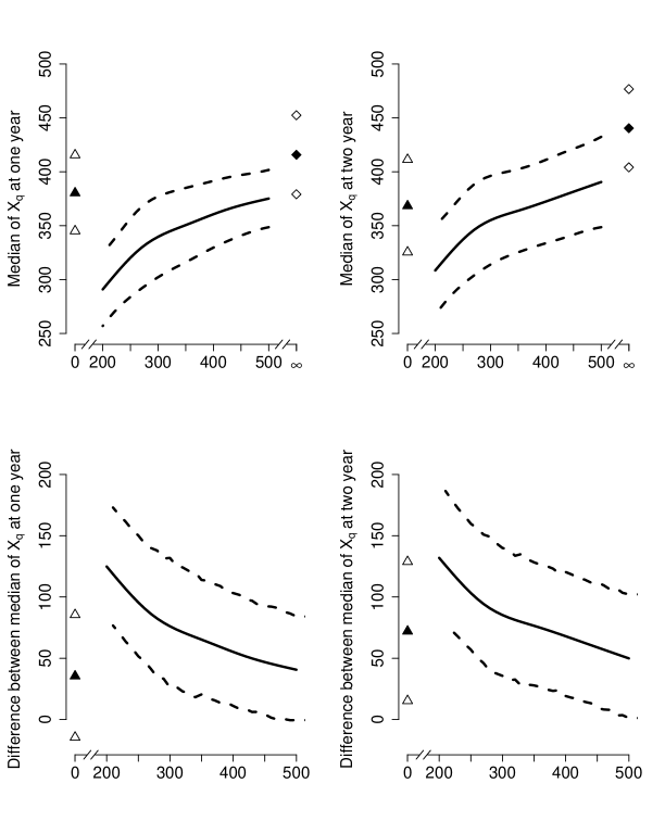
Figure 3: The effectiveness of continuous regimes. The upper panel presents the median of $X_{q}$, $\widehat{\theta}_{q2}$, at one-year and two-years; the bottom panel displays the difference in $\widehat{\theta}_{q2}$ at one-year and two-years between regimes $q=\infty$ and $q\in\{0,200,210,\ldots,500\}$. The triangles represent $\widehat{\theta}_{q2}$ corresponding to regime $q=0$ (upper panel), and the difference in $\widehat{\theta}_{q2}$ between regimes $q=\infty$ and $q=0$ (bottom panel). Similarly, the diamonds correspond to $\widehat{\theta}_{q2}$ under regime $q=\infty$. The filled symbols are the mean values, and the empty symbols are the upper and lower bounds of the 95% confidence intervals.

Finally, we estimate the causal effect of the DTR on the median of $X_{q}$ using the smoothed relationship between $F^{-1}_{X_{q}}({\textstyle\frac{1}{2}})$ and $q$ from model (3). The estimated “dose response” curves of $\widehat{\theta}_{q2}$ versus $q$ appear in the top panel of Figure 3. The bottom panel describes the difference in $\widehat{\theta}_{q2}$ between dynamic regimes $q=\infty$ and $q\in\{0,200,210,\ldots,500\}$. Our results indicate that immediate ART initiation leads to significantly higher median values of the composite outcome $X_{q}$ than delayed ART initiation. Furthermore, as an illustration of increased efficiency, the variance of the one-year outcome associated with $q=350$ estimated from the structural model is 180, compared to 209 for the regime-specific estimate, a 13.9% reduction. The R code used to implement our approaches is available in Supporting Information.

5 Summary and discussion

Motivated by inconclusive evidence for supporting the current WHO guidelines promoting immediate ART initiation in adolescents, we have conducted an analysis comparing dynamic treatment initiation rules. Our approach utilizes the theory of causal inference for DTRs. We extend the framework to allow the causal comparisons of both specific regimes and regimes along a continuum, Additionally, propose strategies to address sparse outcomes and death, and use a composite outcome that can be used to draw causal comparisons between DTRs.

Our analysis suggests that immediate ART initiation leads to mortality benefit and higher median values of the composite outcome, relative to delayed ART initiation. The ‘never treat’ regime yields significantly higher mortality than other initiation rules.

The data from IeDEA pose several challenges that we addressed within our analysis. First, treatment initiation times are recorded on a continuous time scale. Existing approaches have relied primarily on discretization of the time axis to construct inverse probability weights. We have derived a method to construct weights that uses the continuous time information. Similar strategies have been employed in Hu et al. (2018) and Johnson and Tsiatis (2005); see also Lok (2008) for related work in the context of structural nested mean models.

Second, CD4 counts are measured at irregularly spaced times. This creates challenges when the goal is to compare treatment regimes at a specific follow up time, as would be the case with a randomized trial. Moreover, even though our sample comprises those who would be scheduled to have at least two years of follow up, some individuals discontinue follow up prior to that time. These features of the data lead to incomplete observation of CD4 count at the target analysis time and to censoring of death times. To address this issue we have relied on a parametric model for the joint distribution of observed CD4 counts and death times. The CD4 submodel is flexible enough to capture important features of the longitudinal trajectory of CD4 counts, and is used to impute missing observations at the target follow up time. The mortality submodel, which depends explicitly on the CD4 trajectory, is used to impute mortality status at the target estimation time. A limitation of the imputation model is that death and CD4 may depend on HIV viral load, but availability of this variable is limited in our data and therefore not included in the model.

The primary strength of this approach is its ability to handle a complex data set on its own terms, without artificially aligning measurement times. Although imputation-based analyses rely on extrapolating missing outcomes, and both the weight model and imputation model must be correctly specified, a potential advantage of our approach over g-computation is reduced dependence on data extrapolation. There are several possible extensions as well. First, largely due to limitations related to computing, we used a two-step approach to fit our observed-data imputation model rather than a joint likelihood approach. There may be some small biases (Rizopoulos, 2012) introduced by using a two-step rather than fully joint model. Second, the imputation model may not be fully compatible with the weighting model in the sense that we are not constructing a joint distribution of all observed data. Our approach emulates a setting whereby the data imputer and the data analyst are separate: the imputed dataset can be turned over for whatever kind of analysis would be applied to a complete dataset. Empirical checks to our joint model for CD4 and mortality showed no evidence of lack of fit to the observed data (see Supporting Information). To make the models more flexible, it may be possible to employ machine learning methods as in Shen et al. (2017). Finally, developing sensitivity analyses to capture the effects of unmeasured confounding for our model would be a worthwhile and important contribution.

6 Supporting Information

Additional supporting information may be found online in the Supporting Information section at the end of the article.

Table 1: Summary statistics

	$n=1962$
	at $t^{*}=1$ year	at $t^{*}=2$ years
ART initiated	$1286\;(65.5\%)$	$1422\;(72.5\%)$
death	$61\;(3.1\%)$	$80\;(4.1\%)$
CD4 counts per person	1.71	2.64
	Mean (SD) or Count (%)	% missing
CD4	$343.05\;(314.78)$	21.3%
WAZ	$-2.64\;(1.83)$	33.7%
HAZ	$-2.10\;(1.48)$	36.1%
age	$12.21\;(1.41)$	0
male	$863\;(44.0\%)$	0
CDC class		71.6%
mild	$200\;(10.2\%)$
moderate	$73\;(3.7\%)$
severe	$88\;(4.5\%)$
asymptomatic	$196\;(10.0\%)$
person time follow up*	$3.6\;(1.7,6.1)$
∗median (1st, 3rd quartile) in years

Table 2: Comparing effectiveness of specific regimes $q\in\{0,200,350,500,\infty\}$ for $t^{*}=1$ year and $t^{*}=2$ years. $\theta_{q1}=P(X_{q}=0)=F_{X_{q}}(0)$, $\theta_{q2}=F_{X_{q}}^{-1}({\textstyle\frac{1}{2}})$, $\theta_{q3}=E(X_{q}{\,|\,}X_{q}>0)$. 95% confidence intervals are shown below the point estimates.

	0	200	350	500	$\infty$	$\infty$ vs. 500
$t^{*}=1$
$\widehat{\theta}_{q1}$	.050	.018	.017	.020	.012	$-.008$
	(.032, .078)	(.007, .044)	(.008, .038)	(.009, .040)	(.006, .024)	$(-.015,-.001)$
$\widehat{\theta}_{q2}$	381	292	354	375	416	41
	(345, 418)	(260, 324)	(320, 387)	(350, 401)	(381, 451)	(12, 70)
$\widehat{\theta}_{q3}$	416	326	377	401	466
	(380, 453)	(294, 357)	(349, 406)	(373, 429)	(435, 498)
$t^{*}=2$
$\widehat{\theta}_{q1}$	.076	.040	.033	.036	.023	$-.013$
	(014, .037)	(.050, .110)	(.021, .074)	(.019, .059)	(.021, .060)	$(-.023,-.004)$
$\widehat{\theta}_{q2}$	353	303	358	387	438	51
	(304, 402)	(262, 343)	(310, 407)	(341, 434)	(395, 481)	(14, 87)
$\widehat{\theta}_{q3}$	394	345	388	418	484
	(348, 441)	(308, 382)	(352, 423)	(381, 455)	(447, 522)

Figure 2: Comparing the median values of $X_{q}$ under regime $q\in\{0,200,350,500,\infty\}$. Weighted (W) and unweighted (UW) estimates are compared side-by-side.

References

- Aalen et al. (2008) Aalen, O., Borgan, O., and Gjessing, H. (2008). Survival and Event History Analysis: A Process Point of View. New York: Springer Science & Business Media.
- Berk et al. (2005) Berk, D. R., Falkovitz-Halpern, M. S., Hill, D. W., Albin, C., Arrieta, A., Bork, J. M., et al. (2005). Temporal trends in early clinical manifestations of perinatal HIV infection in a population-based cohort. The Journal of the American Medical Association 293, 2221–2231.
- Cain et al. (2010) Cain, L. E., Robins, J. M., Lanoy, E., Logan, R., Costagliola, D., and Hernán, M. A. (2010). When to start treatment? A systematic approach to the comparison of dynamic regimes using observational data. The International Journal of Biostatistics 6(2),.
- Chakraborty and Murphy (2014) Chakraborty, B. and Murphy, S. A. (2014). Dynamic treatment regimes. Annual Review of Statistics and Its Application 1, 447–464.
- Cole and Hernán (2008) Cole, S. R. and Hernán, M. A. (2008). Constructing inverse probability weights for marginal structural models. American Journal of Epidemiology 168, 656–664.
- Daniel et al. (2013) Daniel, R., Cousens, S., De Stavola, B., Kenward, M., and Sterne, J. (2013). Methods for dealing with time-dependent confounding. Statistics in Medicine 32, 1584–1618.
- Egger et al. (2012) Egger, M., Ekouevi, D. K., Williams, C., Lyamuya, R. E., Mukumbi, H., Braitstein, P., et al. (2012). Cohort profile: the International Epidemiological Databases to Evaluate AIDS (IeDEA) in sub-Saharan Africa. International Journal of Epidemiology 41, 1256–1264.
- Hastie et al. (2009) Hastie, T., Tibshirani, R., and Friedman, J. (2009). The Elements of Statistical Learning: Data Mining, Inference, and Prediction. New York: Springer.
- Hernán et al. (2006) Hernán, M., Lanoy, E., Costagliola, D., and Robins, J. (2006). Comparison of dynamic treatment regimes via inverse probability weighting. Basic & Clinical Pharmacology & Toxicology 98, 237–242.
- Hu et al. (2018) Hu, L., Hogan, J. W., Mwangi, A. W., and Siika, A. (2018). Modeling the causal effect of treatment initiation time on survival: Application to HIV/TB co-infection. Biometrics 74, 703–713.
- Johnson and Tsiatis (2005) Johnson, B. A. and Tsiatis, A. A. (2005). Semiparametric inference in observational duration-response studies, with duration possibly right-censored. Biometrika 92, 605–618.
- Leng and Zhang (2014) Leng, C. and Zhang, W. (2014). Smoothing combined estimating equations in quantile regression for longitudinal data. Statistics and Computing 24, 123–136.
- Lok (2008) Lok, J. J. (2008). Statistical modeling of causal effects in continuous time. The Annals of Statistics 36, 1464–1507.
- Luzuriaga et al. (2004) Luzuriaga, K., McManus, M., Mofenson, L., Britto, P., Graham, B., and Sullivan, J. L. (2004). A trial of three antiretroviral regimens in HIV-1–infected children. New England Journal of Medicine 350, 2471–2480.
- Mark et al. (2017) Mark, D., Armstrong, A., Andrade, C., Penazzato, M., Hatane, L., Taing, L., Runciman, T., and Ferguson, J. (2017). Hiv treatment and care services for adolescents: a situational analysis of 218 facilities in 23 sub-saharan african countries. Journal of the International AIDS Society 20, 21591.
- Moodie et al. (2007) Moodie, E., Richardson, T., and Stephens, D. (2007). Demystifying optimal dynamic treatment regimes. Biometrics 63, 447–455.
- Rizopoulos (2012) Rizopoulos, D. (2012). Joint Models for Longitudinal and Time-to-Event Data: With Applications in R. Boca Raton, FL: CRC Press.
- Robins (1986) Robins, J. (1986). A new approach to causal inference in mortality studies with a sustained exposure period application to control of the healthy worker survivor effect. Mathematical Modelling 7, 1393–1512.
- Robins et al. (2008) Robins, J., Orellana, L., and Rotnitzky, A. (2008). Estimation and extrapolation of optimal treatment and testing strategies. Statistics in Medicine 27, 4678–4721.
- Rubin (1987) Rubin, D. B. (1987). Multiple Imputation for Nonresponse in Surveys. New York: John Wiley & Sons.
- Schomaker et al. (2017) Schomaker, M., Leroy, V., Wolfs, T., Technau, K. G., Renner, L., Judd, A., et al. (2017). Optimal timing of antiretroviral treatment initiation in HIV-positive children and adolescents: a multiregional analysis from Southern Africa, West Africa and Europe. International Journal of Epidemiology 46, 453–465.
- Shen et al. (2017) Shen, J., Wang, L., and Taylor, J. M. (2017). Estimation of the optimal regime in treatment of prostate cancer recurrence from observational data using flexible weighting models. Biometrics 73, 635–645.
- Violari et al. (2008) Violari, A., Cotton, M. F., Gibb, D. M., Babiker, A. G., Steyn, J., Madhi, S. A., et al. (2008). Early antiretroviral therapy and mortality among HIV-infected infants. New England Journal of Medicine 359, 2233–2244.
- WHO (2015) WHO (2015). Guideline on when to start antiretroviral therapy and on pre-exposure prophylaxis for HIV. World Health Organization.