Polymer stress growth in viscoelastic fluids in oscillating extensional flows with applications to micro-organism locomotion

Abstract

Simulations of undulatory swimming in viscoelastic fluids with large amplitude gaits show concentration of polymer elastic stress at the tips of the swimmers.We use a series of related theoretical investigations to probe the origin of these concentrated stresses. First the polymer stress is computed analytically at a given oscillating extensional stagnation point in a viscoelastic fluid. The analysis identifies a Deborah number (De) dependent Weissenberg number (Wi) transition below which the stress is linear in $\textrm{Wi},$ and above which the stress grows exponentially in $\textrm{Wi}.$ Next, stress and velocity are found from numerical simulations in an oscillating 4-roll mill geometry. The stress from these simulations is compared with the theoretical calculation of stress in the decoupled (given flow) case, and similar stress behavior is observed. The flow around tips of a time-reversible flexing filament in a viscoelastic fluid is shown to exhibit an oscillating extension along particle trajectories, and the stress response exhibits similar transitions. However in the high amplitude, high De regime the stress feedback on the flow leads to non time-reversible particle trajectories that experience asymmetric stretching and compression, and the stress grows more significantly in this regime. These results help explain past observations of large stress concentration for large amplitude swimmers and non-monotonic dependence on De of swimming speeds.

1 Introduction

Simulations of swimming in viscoelastic fluids involving large amplitude gaits [20, 23, 18] show substantially different swimming speeds than those found in low amplitude simulations and asymptotic analyses [4, 5, 10, 6, 16, 3]. Concentration of polymer elastic stress at the tips of slender objects has been seen in numerical simulations of flagellated swimmers in viscoelastic fluids [20, 22, 23, 12], and it is thought that the presence of these large stresses is related to the observed differences in behavior at low and high amplitude. We recently explained the origin of the stress concentration at the tips of steady, translating cylinders [13]. The tips of swimmers, however, experience unsteady oscillating motion. This paper analyzes oscillatory extensional flows, which are similar to the flows around bending objects, and it identifies parameter regimes which lead to the presence of large concentrated stresses.

In Fig. 1 we present results similar to those from [22, 23] which compare low and high amplitude undulatory swimmers in a 2D Stokes-Oldroyd-B fluid. In Fig. 1 (a)-(b) we show the scaled strain energy density (trace of the stress) for both low and high Deborah number and amplitude. The Deborah number is the polymer relaxation time scaled by the flow time-scale, and is denoted by $\textrm{De}.$ Large stress accumulation at the tail only occurs in the high $\textrm{De},$ high amplitude case. In Fig. 1(c)-(d) we plot the maximum strain energy density and swimming speed (normalized by the swimming speed in a Newtonian fluid) as a function of $\textrm{De}.$ In both the stress response and normalized swimming speed, the high amplitude behavior is very different from the low amplitude behavior at high $\textrm{De}.$ At low $\textrm{De},$ low and high amplitude motion results in similar normalized swimming speed, but significant slow downs are seen for the high amplitude swimmers where the stress is also very high.

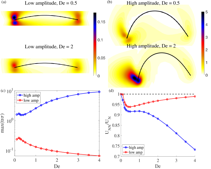
Figure 1: (a,b) Snapshots of the stress distributions around swimmers with (a) low and (b) high amplitude gaits at both low and high Deborah numbers (De). The swimmer gait is prescribed with a curvature $\kappa(s,t)=\left(A_{t}(1-s)+A_{h}s\right)\sin(2\pi t+\pi s),$ where $(A_{t},A_{h})$ are the tail and head curvature amplitudes, and $(A_{t},A_{h})=(5,2)$ for the large amplitude case and $(1,2/5)$ for low amplitude. The color field shows polymer strain energy density scaled by $2\mu_{p}A_{t}.$ A similar scaling will be used for the flexors in Sec. 5. (c) Scaled strain energy density in a neighborhood near the tail as a function of $\textrm{De}.$ (d) Non-Newtonian swimming speed normalized by swimming speed in a Newtonian fluid.

Translating cylinders in a viscoelastic fluid exhibit a Weissenberg number transition from low to high stress concentration at the cylinder tips [13]. The Weissenberg number, $\textrm{Wi},$ is the polymer relaxation time scaled by the flow strain rate. This transition is similar to the coil-stretch transition found for viscoelastic fluids at steady extensional points. Undulatory swimmers are oscillating as well as translating, and the Deborah number is typically reported as the relevant non-dimensional relaxation time in this case. Here we show that the fluid near tips of oscillating filaments in 2D experience oscillating extension along particle trajectories, and both Deborah number and Weissenberg number are important. Our results extend known transitions in Wi at steady extensional stagnation points to oscillating extensional points, and the Wi transition becomes De dependent in this case. The need to report both De and Wi has been well appreciated in the engineering community, see [2, 15] for nice discussions of these two parameters, but it has not been noted before in the context of micro-organism locomotion in viscoelastic fluids.

In this paper we analyze the stress response at a fixed oscillatory extensional stagnation point with no stress feedback on the flow. We compare these analytical results with different numerical simulations in which the stress and flow are coupled. We examine flow-stress coupling in oscillating extension by forcing the flow with a 4-roll mill background force that is oscillatory in time. Next, we look at the flow around flexing filaments with a time-reversible oscillation of a circular arc of a given amplitude. The flow around these so-called flexors is similar to the flow around undulatory swimmers and provides a connection between the analysis of stress response at oscillatory extensional stagnation points and recent numerical studies on stress accumulation at tips of flagellated and undulatory swimmers [20, 22, 17, 24, 12].

2 Model Equations

We use the Oldroyd-B model of a viscoelastic fluid in the zero-Reynolds number limit. The Oldroyd-B model is the simplest model of a viscoelastic fluid which captures elastic effects such as storage of memory from past deformation on a characteristic time-scale $\lambda.$ We study zero-Reynolds number because this work is motivated by micro-organism locomotion. The model equations for velocity $\textbf{u},$ pressure $p,$ and polymer stress tensor $\boldsymbol{\tau}$ are

$$-\nabla p+\mu_{s}\Delta\textbf{u}+\nabla\cdot\boldsymbol{\tau}+\mathbf{f}=0$$ (1)

$$\nabla\cdot\textbf{u}=0$$ (2)

$$\boldsymbol{\tau}+\lambda\stackrel{{\scriptstyle\nabla}}{{\boldsymbol{\tau}}}=2\mu_{p}\dot{\boldsymbol{\gamma}},$$ (3)

where $\stackrel{{\scriptstyle\nabla}}{{\boldsymbol{\tau}}},$ denotes the upper convected derivative, and is defined by

$$\stackrel{{\scriptstyle\nabla}}{{\boldsymbol{\tau}}}=\partial_{t}\boldsymbol{\tau}+\textbf{u}\cdot\nabla\boldsymbol{\tau}-\left(\nabla\textbf{u}\boldsymbol{\tau}+\boldsymbol{\tau}\nabla\textbf{u}^{T}\right).$$ (4)

The solvent and polymer viscosities are $\mu_{s},$ and $\mu_{p}$, respectively, and $\dot{\boldsymbol{\gamma}}=\left(\nabla\textbf{u}+\nabla\textbf{u}^{T}\right)/2$ is the rate of strain tensor. The function $\mathbf{f}$ is the external forcing that drives the system, and will be given explicitly for the different examples in Sec. 4 for the 4-roll mill geometry and in Sec. 5 for the flexor simulations.

3 Stress response to oscillating extension with no coupling

It is well known that in the Oldroyd-B model of a viscoelastic fluid, the stress shows unbounded exponential growth at extensional points when stretching outpaces relaxation. The rapid stretching originates from the nonlinearity in the upper-convected derivative, Eq. (4). This derivative is the frame-invariant material derivative of a tensor, or derivative of a tensor along a particle path, making it essential in continuum models of viscoelastic fluids. Other similar models such as Giesekus, FENE-P, and PTT also lead to large concentrated stresses in these regions of strong extension [9]. We use the Oldroyd-B model here because it is the simplest model that contains these nonlinear features and is amenable to analysis.

We begin by repeating the well known calculation for stress divergence in the Oldroyd-B model for a fixed velocity, in order to frame the following sections. Consider a linear extensional flow $\textbf{u}=\alpha(x,-y)$ for $\alpha>0$. At the origin, the diagonal components of the stress satisfy

$$\lambda\frac{d}{dt}\boldsymbol{\tau}_{11} =\phantom{-}2\alpha\mu_{p}-(1-2\lambda\alpha)\boldsymbol{\tau}_{11}$$ (5)

$$\lambda\frac{d}{dt}\boldsymbol{\tau}_{22} =-2\alpha\mu_{p}-(1+2\lambda\alpha)\boldsymbol{\tau}_{22}.$$ (6)

For $2\lambda\alpha<1$, the stress approaches a bounded steady state, and for $2\lambda\alpha>1$, $\boldsymbol{\tau}_{11}$ grows exponentially in time without bound. For this flow, the Weissenberg number is $\textrm{Wi}=2\alpha\lambda$, and the unbounded stress growth occurs for $\textrm{Wi}>1.$

We extended this classical result to the situation in which the strength of extension is oscillating in time with mean zero and period $T$. Specifically, we assume a velocity field (independent of the stress) of the form

$$\textbf{u}=\alpha h(t/T)(x,-y),$$ (7)

where $h(t)$ is a periodic function with period $1$, mean zero, and maximum 1. At the origin, the diagonal components of the stress satisfy the following ODE’s:

$$\lambda\left(\frac{d}{dt}\boldsymbol{\tau}_{11}-2\alpha h(t/T)\boldsymbol{\tau}_{11}\right)+\boldsymbol{\tau}_{11} =\phantom{-}2\alpha\mu_{p}h(t/T)$$ (8)

$$\lambda\left(\frac{d}{dt}\boldsymbol{\tau}_{22}+2\alpha h(t/T)\boldsymbol{\tau}_{22}\right)+\boldsymbol{\tau}_{22} =-2\alpha\mu_{p}h(t/T).$$ (9)

We nondimensionalize these equations by scaling stress by $2\mu_{p}\alpha$ and scaling time by the period $T$. We denote the dimensionless stress by $\boldsymbol{\sigma}=\boldsymbol{\tau}/2\mu_{p}\alpha$. The dimensionless equations are

$$\textrm{De}\;\frac{d}{dt}\boldsymbol{\sigma}_{11}+(1-h(t)\textrm{Wi})\;\boldsymbol{\sigma}_{11} =\phantom{-}h(t)$$ (10)

$$\textrm{De}\;\frac{d}{dt}\boldsymbol{\sigma}_{22}+(1+h(t)\textrm{Wi})\;\boldsymbol{\sigma}_{22} =-h(t),$$ (11)

where, as before, the Weissenberg number is $\textrm{Wi}=2\alpha\lambda,$ and the Deborah number is $\textrm{De}=\lambda/T$.

To gain insight from an analytic solution to these equations, we choose the function $h$ to be the square wave

$$h(t)=\begin{cases}\phantom{-}1&\text{for }\text{mod}(t,1)\leq 1/2\\ -1&\text{for }\text{mod}(t,1)>1/2\end{cases}.$$ (12)

This choice of $h$ permits us to find the periodic solution analytically, from which we compute the maximum in time of the trace of the stress (strain energy density) as

$$\max{\rm tr}\;\boldsymbol{\sigma}=\frac{2\sinh\left(\frac{\textrm{Wi}}{2\textrm{De}}\right)-2\textrm{Wi}\sinh\left(\frac{1}{2\textrm{De}}\right)}{(\textrm{Wi}^{2}-1)\sinh\left(\frac{1}{2\textrm{De}}\right)}.$$ (13)

Unlike the case of steady extensional flow, the solution remains bounded in time, and it approaches a periodic solution for all Wi.

Figure 2(a) shows how the stress depends on Wi for different fixed De. This plot shows two different regimes for how the stress depends on Wi, and there is a Deborah number dependent transition between the two regimes. To understand the behavior in the two regimes, we expand the max trace of the stress in the limits of large and small Wi. For small Wi, the max trace stress scales linearly with Wi:

$$\max{\rm tr}\;\boldsymbol{\sigma}\sim\left(\frac{2\textrm{De}\sinh\left(\frac{1}{2\textrm{De}}\right)-1}{\textrm{De}\sinh\left(\frac{1}{2\textrm{De}}\right)}\right)\textrm{Wi},\quad\textrm{for }\textrm{Wi}<<1.$$ (14)

For large Wi, the max trace of the stress to leading order is

$$\max({\rm tr}\;\boldsymbol{\sigma})\sim\left(\frac{1}{\sinh\left(\frac{1}{2\textrm{De}}\right)}\right)\frac{\exp\left(\frac{\textrm{Wi}}{2\textrm{De}}\right)}{\textrm{Wi}^{2}},\quad\textrm{for }\textrm{Wi}>>1.$$ (15)

This expansion is generated by assuming not only that Wi is large, but also that Wi is large compared to De. Thus the transition from the low Weissenberg number regime to the high Weissenberg number regime depends on the Deborah number. In Figure 2(a) we include plots of the asymptotic expressions for the stress for both high and low Wi for $\textrm{De}=0.5$. The transition for the linear behavior to the exponential behavior appears to occur somewhere between $\textrm{Wi}=2$ and $\textrm{Wi}=4.$

For fixed Wi, the stress is a decreasing function of De. The case of $\textrm{De}=0$ corresponds to the steady extension case. For high De, the duration of stretch is short, and the stresses do not get very large before the flow changes to compression.

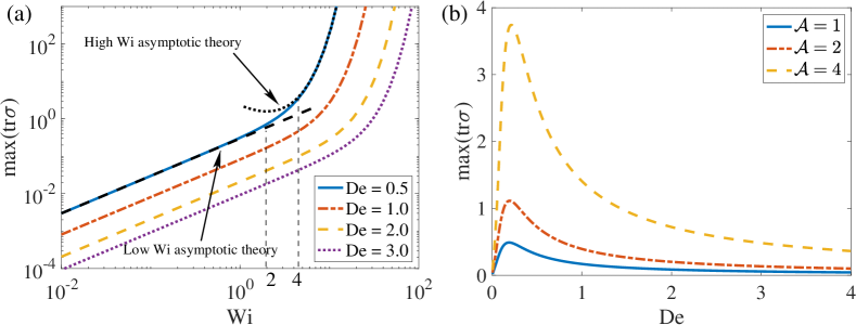
Figure 2: (a) Analytical solution of $\max({\rm tr}\;\boldsymbol{\sigma})$ as a function of Wi for $\textrm{De}=0.5,1,2,3$ at oscillatory extensional stagnation points with no stress feedback in the Stokes-Oldroyd-B model. Linear and exponential asymptotic approximations are included to highlight transition. Wi transition depends on $\textrm{De}.$ (b) Analytical solution of $\max({\rm tr}\;\boldsymbol{\sigma})$ as a function of De for non-dimensional stretch rate $\mathcal{A}=1,2,4.$

With this nondimensionalization both Wi and De scale with the relaxation time. In studies of locomotion, it is useful consider how the speed depends on De for a given gait. Similarly, in Section 5, we consider how the stress depends on relaxation time as an object changes shape with a fixed amplitude. For such problems, it is useful to consider how the stress depends on the nondimensional stretch rate $\mathcal{A}=\alpha T=\textrm{Wi}/(2\textrm{De})$ in place of Wi. This other parameter captures the amplitude of the stretching independent of the relaxation time, and the relaxation time only appears in De. For this nondimensionalization $\textrm{De}=0$ corresponds to Newtonian flow.

In Fig. 2(b) we plot the max of the trace of the stress a function of De for a range of stretch rates $\mathcal{A}=1,2,4$. As De goes to either $0$ or $\infty$, the stress goes to zero, and as a result the stress is a nonmonotonic function of De. The De where the peak stress occurs is fairly insensitive to the stretch rate within the ranges of $\mathcal{A}$ presented.

In C we present results of a numerical solution to Eqs. (10)–(11) for the Giesekus model to demonstrate how additional nonlinear terms effect the theory developed in this section.

4 Stress response to oscillating extension with coupling

The analysis from the previous section considered the flow fixed independent of the stress. Here we examine an oscillating extensional flow in which the stress and velocity are coupled. We drive the system by prescribing a 4-roll mill type background body force and solve for the resulting velocity and stress numerically and compare the results with those from the previous section.

We adapt the model problem from [25, 9] in which the stress at steady extensional points was examined numerically. Specifically, we solve the Stokes-Oldroyd-B equations, Eqs. (1)-(3) on the two-dimensional periodic domain $[-\pi,\pi]^{2}$ with a driving background body force

$$\mathbf{f}=2\alpha\sin\left(2\pi t/T\right)\left(\begin{array}[]{l}-\sin x\cos y\\ \phantom{-}\cos x\sin y\end{array}\right).$$ (16)

Note in the stokes limit ($\lambda=0$) this body force drives the flow $\textbf{u}=-\mathbf{f}/2$. At the origin the linearized flow is identical to the flow defined in equation (7) from the decoupled problem with $h(t)=\sin\left(2\pi t\right)$.

The system is solved with a pseudo-spectral method for spatial derivatives and a 2nd order implicit-explicit time integrator; small stress diffusion is added to control stress gradients. See A for details on the numerical method and discretization parameters.

As before, the Deborah number is $\textrm{De}=\lambda T$. The Weissenberg number is computed as $\textrm{Wi}=\lambda\dot{\gamma}$ where $\dot{\gamma}=\max_{t}\sqrt{2\dot{\boldsymbol{\gamma}}:2\dot{\boldsymbol{\gamma}}/2}$ for $\dot{\boldsymbol{\gamma}}$ measured at the origin once the solution has equilibrated to the periodic solution. For a Newtonian fluid $\dot{\gamma}=2\alpha,$ but we find that even for viscoelastic fluids in the highly nonlinear regime of large stresses $\dot{\gamma}\approx 2\alpha$. Hence for this problem one can use $\textrm{Wi}=2\alpha\lambda$ and nondimensionalize the polymer stress by $\boldsymbol{\sigma}=\boldsymbol{\tau}/(2\mu_{p}\alpha)$, which is equivalent to what was done in the previous section.

In Fig. 3 we show ${\rm tr}\;\boldsymbol{\sigma}$ near the origin (on part of the simulation domain: $[-\pi/2,\pi/2]^{2}$) for 8 different times over one period for $\textrm{Wi}=12$ and $\textrm{De}=1/2$ after the solution has reached the periodic solution. These plots show the large stresses switching orientation over the course of a period due to the alternating directions of stretching. At the beginning of the period (t=0) the stress is oriented in the horizontal direction, but at this time, the flow begins stretching in the vertical direction and compressing in the horizontal direction. Over the next half period, the stress becomes increasingly oriented in the vertical direction. Over the second half of the period, the flow stretches in the horizontal direction and compresses in the vertical direction.

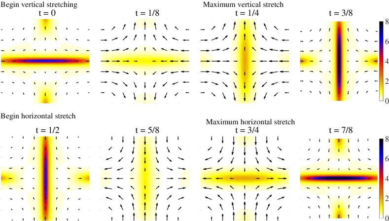
Figure 3: Velocity field overlayed on colorfield displaying polymer strain energy density over one period for oscillating extension near the origin on the domain $[-\pi/2,\pi/2]^{2}$ for the fully coupled 4-roll mill simulations, at $\textrm{De}=0.5,$ $\textrm{Wi}=12.$

To compare the results of the fully coupled simulations with the theory presented in Sec. 3 we numerically solve the ODE’s in Eqs. (10)-(11) with temporal oscillation $h(t)=\sin(2\pi t).$ We note that there is no closed form analytic expression such as Eq. (13) for a sinusoidal oscillation. This is the analog of the coupled 4-roll mill at the origin, but in the decoupled limit, i.e. where the stress does not affect the velocity. In Fig. 4 we examine plots of $\max({\rm tr}\;\boldsymbol{\sigma})$ as a function of dimensionless parameters in both the coupled case as well as in the decoupled case. The behavior of the stress with sinusoidal temporal oscillation is qualitatively the same as that of the square-wave oscillation. As before, the stress as a function of Wi shows two regimes: a low Wi regime in which the stress is a linear function of Wi, and a high Wi regime in which the stress dependence on Wi is exponential. The Wi at the transition between these two regime again depends on De. The agreement between the decoupled and coupled cases is quite good, but in the high $\textrm{Wi},$ low De regime, where the largest stresses are expected, there is disagreement. In this problem we find that the non-linear coupling has the effect of reducing the stress rather than enhancing it. This is consistent with what was found in [25] where the nonlinearities modified the flow and also reduce the stress.

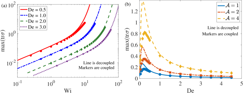
Figure 4: Max polymer strain energy density at the origin in the decoupled ODE (line) and the 4-roll mill coupled simulations (markers) as a function of Wi for fixed De (a), and as a function of De for fixed $\mathcal{A}$ in (b).

5 Flows around flexing objects

5.1 Bending, no translation

In order to simplify the study of the flows around the tips of undulatory swimmers we consider filaments of length $L=1$ oscillating through circular arcs with peak curvature $A$. Specifically, the curvature is

$$\kappa(s,t)=A\sin\left(\frac{2\pi}{T}t\right).$$ (17)

For $A=\pi$ the fully bent shape is a semi-circle. We consider low amplitude $A\approx 1$ and high amplitude $A\approx 4$; see Fig. 5. By symmetry, this motion does not result in any horizontal translation of the body. We refer to these non-translating “swimmers” as flexors. We previously used these objects to study the effect of viscoelasticity on soft swimmers in [23]. In what follows we solve Eqs. (1)-(3), and the external force density, $\mathbf{f}$ is used to enforce the prescribed shape of the swimmer. The method is similar to [12] where the shape is given and the system is solved under the constraint that it is force and torque free. Thus the flexor has a fixed shape, but it is free to move in the fluid. Details of the numerical method are given in B. This method is different from previous swimmer simulations [20, 22, 17, 23] which enforced a prescribed shape approximately using forces that penalized deviations from a target curvature.

In the flexor model the Deborah number is defined as $\textrm{De}=\lambda/T,$ where $T$ is the period of motion of the flexor. Defining a Weissenberg number is more complicated than in the 4-roll mill. Because the strain rate varies significantly at different places in the flow, it is not clear how to define a characteristic $\dot{\gamma}.$ In a region near the tip we find that $\dot{\gamma}\propto A$ with constant of proportionality $\approx 2,$ and hence we define $\textrm{Wi}=2\lambda A,$ and scale the polymer stress as $\boldsymbol{\sigma}=\boldsymbol{\tau}/(2\mu_{p}A)$. This is consistent with the scalings in Sec. 3 and 4. We give more evidence for $\dot{\gamma}\approx 2A$ in what follows.

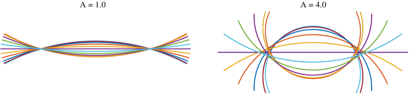
Figure 5: Prescribed shapes for low and high amplitude flexors.

In Fig. 6 (a) we plot the strain energy density ${\rm tr}\;\boldsymbol{\sigma}$ for low amplitude ($A=0.5$) and high amplitude ($A=5)$ flexors during the downstroke of the motion for $\textrm{De}=1.$ All results are shown after the flow has equilibrated to a periodic state at $t\approx 10\lambda.$ We note that the stress is localized at the tips of the flexors during the motion. It has a much larger scale for the large amplitude case. The spatial distribution of stress is more symmetric about the flexor for the low amplitude case than in the high amplitude case. The low amplitude case corresponds to $\textrm{Wi}=1$ and the high amplitude case corresponds to $\textrm{Wi}=10.$ Suggested by the theory developed for pure oscillating extension, shown in Fig. 4(a), the values $\textrm{Wi}=1,\;\textrm{De}=1$ are well in the linear regime, whereas $\textrm{Wi}=10,\textrm{De}=1$ are in the transition region between linear to exponential.

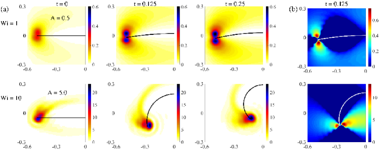
Figure 6: (a) Polymer strain energy density (${\rm tr}\;\boldsymbol{\sigma}$) around flexors at $\textrm{Wi}=1$ and $\textrm{Wi}=10$ with $\textrm{De}=1,$ corresponding to low ($A=0.5$) and high ($A=5.0$) amplitude flexors at different times during a period. (b) Maximum stretch rate $\nu$ for low and high amplitude flexors.

To understand why the stress concentrates preferentially near the tips of the flexors we examine the flow near the tips. In [13] we showed that stretching near the tips of translating cylinders led to large concentrated stresses beyond a critical Wi. To identify the critical Wi, we identified a quantity called the maximum stretch rate as the maximum real part of the eigenvalues of the operator $\mathcal{S}[\textbf{u}]\mathbf{C}\equiv\left[\nabla\textbf{u}\mathbf{C}+\mathbf{C}\nabla\textbf{u}^{T}\right].$ The term $\mathcal{S}[\textbf{u}]\boldsymbol{\tau}$ arises in the upper-convected Maxwell equation, Eq. (3), and the eigenvalues of $\mathcal{S}[\textbf{u}]$ define the define the growth (or decay) rates of stress due to stretching (or compression) along particle paths. The solution to the eigenvalue problem $\mathcal{S}[\textbf{u}]\mathbf{C}=\nu\mathbf{C}$ is $\mathbf{C}=\mathbf{v}_{i}\mathbf{v}_{j}^{T},$ $\nu_{ij}=\mu_{i}+\mu_{j},$ where $\mu_{i}$ is an eigenvalue of $\nabla\textbf{u}$ with corresponding eigenvector $\mathbf{v}_{i}.$ We define the maximum stretch rate $\nu$ at a point defined by

$$\nu=2\max(\textrm{Re}(\Lambda(\nabla\textbf{u}))),$$ (18)

where $\Lambda(A)$ is the set of eigenvalues of the matrix $A.$ The max stretch rate is related to the shear rate $\dot{\gamma}$, but it quantifies specifically the rate of local extension where the nonlinearities in the stress evolution equation are significant. In Fig. 6 (b) we plot the max stretch rate for low and high amplitude motion when the flexor is in the middle of the downstroke. It is clear that the highly extensional regions of the flow are at the tips for low and high amplitude flexors.

We examine the flow near the tips by following particle paths in the Newtonian flow. In Fig. 7 (a)-(b) we highlight a portion of the particle path near the tip for low and high amplitude flexors. To measure the strain rate near the tip we first take the average $\dot{\gamma}$ over a set of trajectories which begin at $t=0$ in a square just above the tip of the flexor of width $\approx.05L.$ In Fig. 7 (c) we plot this average $\dot{\gamma}(t)/A$ over one period. In this region the strain rate is oscillating periodically between $\pm 2A,$ i.e. $\dot{\gamma}\sim 2A\sin(t/T).$ The temporal maximum of $\dot{\gamma}$ averaged in the neighborhood near the tip is plotted in Fig. 7 (d) over a range of amplitudes. A linear fit to the data gives a slope of $1.98.$

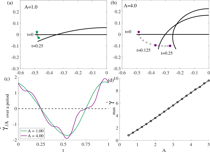
Figure 7: Flexor motion and particle path for point near tip for $A=1$ (a) and $A=4$ (b) flexors in a Newtonian fluid. (c) Rate of strain (averaged near tip of flexor) over a period scaled by $A$ for $A=1,4$ in a Newtonian fluid. (d) Maximum shear rate averaged over a region near the tip is proportional to the amplitude with proportionally constant approximately 2.

To examine the direction of stretching, in Fig. 8 we plot the eigenvectors with positive eigenvalue of the strain rate tensor, $\dot{\boldsymbol{\gamma}}$, scaled by the eigenvalue over a period on a particle trajectory that begins slightly above the flexor. In these plots the dots are equally spaced in time and hence indicate speed of motion. The red dots correspond to the down stroke and the blue are the upstroke. The three additional highlighted times in each portion of the motion correspond to eighths of a period, with $t=1/4,3/4$ when the flow is at rest. It is notable that the direction of stretching on the downstroke is perpendicular to the direction of motion on the upstroke, which is indicative of an oscillating extensional flow. Unlike the problems analyzed in the previous sections, there is some rotation of the stretching direction. Also note that the high amplitude case has a more complicated path as well as a longer path relative to the amplitude. Although the trajectories change for different initial position these are representative of a region of points in the fluid above (or below) the flexor near the tip. Thus we conclude that near the tip the fluid particles are experiencing an oscillating extension in this region along with some rotation.

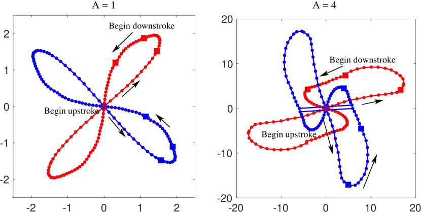
Figure 8: Amplitude and direction of principle stretch given by eigenvectors and eigenvalues of $\dot{\boldsymbol{\gamma}}$ in a Newtonian fluid over a period along a particle path near the tip for low and high amplitude flexors.

To compare the results of stress response for flexors with the analytic solution and 4-roll simulations we quantify the polymer stress around the flexor tip. We define $\max({\rm tr}\;\boldsymbol{\sigma})$ by averaging over trajectories, similar to how we defined $\dot{\gamma}$ in Fig. 7 (d). For $\boldsymbol{\sigma}$ we choose the location of the patch of fluid over which the average is taken to be centered on the spatio-temporal maximum of $\boldsymbol{\sigma},$ and we use a patch size $0.1L.$ (Note that now we average over a patch size that is double the size used to define the stretch rate to account for the symmetry breaking that occurs with fluid elasticity. We include regions above and below the tip.) With the region specified, we define $\max({\rm tr}\;\boldsymbol{\sigma})$ as the spatial average of the maximum in time of ${\rm tr}\;\boldsymbol{\sigma}$ on this region.

We plot $\max({\rm tr}\;\boldsymbol{\sigma})$ for a range of De and Wi in Fig. 9. In order to compare with the theory from Sec. 4 we also plot the theoretical predictions for the stress at the oscillating extensional point on Fig. 9. The solid lines come from the theory for the decoupled oscillating extensional flow with sinusoidal temporal forcing, and the markers are results of simulations of flexors.

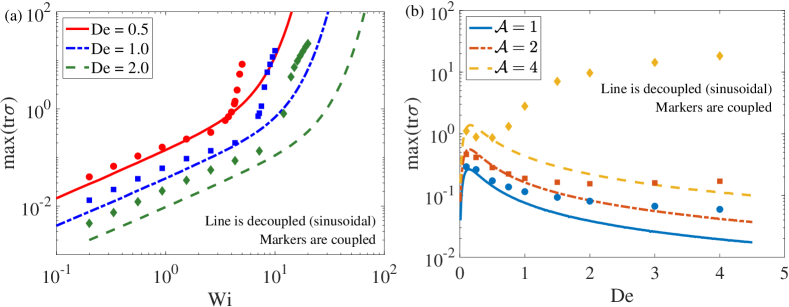
Figure 9: Polymer strain energy density for flexors (markers) and decoupled theory with sinusoidal forcing (lines). (a) Stress dependence on Wi for a range of De (b) Stress dependence on De for a range of $\mathcal{A},$ the non-dimensional “gait”.

The stress as a function of Wi from Fig. 9 again shows linear behavior at low Wi and exponential at high Wi for the flexor. At low Wi and low De the stress is similar to the decoupled theory, but generally the stress response is significantly larger for the flexor simulations than from the theory. Note that while the stress response is stronger for the flexors than the theory predicts, the theory is still able to capture the location of the transition fairly well; the large stress growth appears near the bend in the theory curve.

The deviation from the decoupled theory (and 4-roll mill simulations) is more pronounced when examining the stress as a function of $\textrm{De},$ for a range of $\mathcal{A}=\textrm{Wi}/(2\textrm{De})$, which, as before, is the nondimensional stretch rate and is proportional to the amplitude. As shown in Fig. 9 (b), for low amplitude there is qualitatively similar stress dependence on De for different $\mathcal{A}$. However, for the high De regime the stress is much larger than in the theory or in the four-roll simulations. Notably, for the highest amplitude, the stress is increasing as a function of De, which is a fundamentally different behavior than in the other problems.

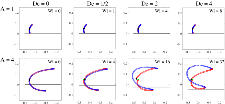
Figure 10: Particle trajectories over one period for flexors at low and high amplitude. Particles start at green diamond and end at black square. Color indicates when the flexor is in the upstroke (red) or downstroke (blue). Grey line is flexor initial position.

To demonstrate why the high amplitude/high De flexors exhibit such different stress response than the theory, in Fig. 10 we plot the trajectories of points near the tips of the flexors for low and high amplitudes at a range of De. The Wi range here is $\textrm{Wi}=0,1,4,8$ for low amplitude and $\textrm{Wi}=0,4,16,32$ for high amplitude. In the large amplitude case, the feedback on the flow from the viscoelastic stresses changes particles paths to make non time-reversible trajectories. The results is that the fluid particles do not feel equal stretching/compression as they do when the path is time-reversible. These fluid particles no longer experience mean zero stretching, and the result is large stress accumulation. Thus the high $\textrm{De},$ high Wi deviation from the theory is a result of nonlinear feedback, which is very different from the affect of such feedback in the four-roll mill simulations where the extensional point was fixed in space.

5.2 Undulatory Swimmer

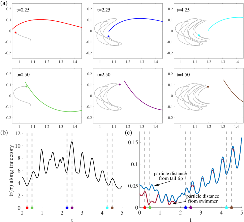
Figure 11: (a) Large amplitude swimmer ($(A_{t},A_{h})=(5,2)$) at 6 snapshots during 5 periods of motion (swimmer is moving left to right, frame is held fixed). Particle path-lines indicate position of particle in the flow over time. (b) Trace of polymer stress at the particle point indicated in (a) over 5 periods. (Snapshot times indicated by corresponding color and dashed lines.) (c) Distance from particle to tail tip and distance from particle to swimmer over time.

Here we explore the relevance of the previous results to a swimmer which is bending and translating.It has been observed that large polymer stress islands concentrate near tips of swimmers [20, 22, 24]. We demonstrated this stress concentration in Fig. 1(b), and using the observations from Sec. 5.1 that relate curvature to $\textrm{Wi},$ we compute $\textrm{Wi}=2\mathcal{A}\textrm{De}\approx 5,$ and $\textrm{Wi}\approx 20$ for $\textrm{De}=0.5$, and $2$ respectively, based on tail curvature amplitude $A_{t}=5.$ In Fig. 11 (a) we show 6 snapshots of the large amplitude swimmer with a representative particle and path-line over 5 periods as the particle moves around the tip. This swimmer has the same gait as the swimmer in Fig. 1(b), and here $\textrm{De}=2.$ In Figs. 11 (b)-(c) we plot the polymer stress at that particle point (in (b)) and both the distance between the particle and the tip as well as the distance between the particle and the swimmer (in (c)) over the 5 periods. We note that over these 5 periods the polymer stress increases as the particle moves closer to the tip and decreases as the particle moves away from the tip. When translation is included any single particle only remains near the tip for a few periods, however there are new particles entering the tip region and experiencing the large stretch and this is sufficient to maintain a large polymer stress patch in the tail region over time.

6 Conclusions

We extend the well-known Wi transitions in steady extension to oscillatory extension, and unlike steady extension we find that bounded solutions exist for all $\textrm{Wi},$ but there is a De dependent Wi transition beyond which the size of the stress grows exponentially in $\textrm{Wi}.$ In simulations of swimmers in the high amplitude, high De case from Fig. 1(b) the swimmer is well in the nonlinear regime at $\textrm{Wi}=20$ and $\textrm{De}=2.$ Comparing the stress as a function of De for swimmers and flexors from Fig. 1(c) and Fig. 9(b), respectively, shows a similar amplitude dependent response, which is different from the theory and simulations of stationary extensional points. Previous simulations [20, 24] noted that swimming speed dependence on De was different for high and low amplitude gaits. Here we explain these observations by identifying a Wi transition which shows that high amplitude gaits operate in the regime of large stress growth.

Both the oscillatory extension stagnation point theory and the 4-roll mill simulations exhibited non-monotonicity in the stress response for a fixed “gait” ($\mathcal{A}=\textrm{Wi}/(2\textrm{De})$). This non-monotonicity comes from the fact that in the limit as $\textrm{De}\rightarrow 0,$ the stress must go to zero, and as $\textrm{De}\rightarrow\infty$ oscillations are averaged out and the stress again goes to zero. For flexors we saw a similar non-monotonicity at low amplitude, but at higher amplitudes we saw that particle paths were deformed and thus the stress growth and decay were no longer averaging out. This non-monotonicity appears to be related to non-monotonic speed responses that have been observed, but not explained, in simulations [20, 22, 17, 24] (also shown in Fig. 1(d)).

For the flexors at high $\textrm{De},$ the stress growth and decay do not average out as they do in the four-roll mill because the systems are driven differently. In the 4-roll mill system, the steady extensional point is driven by a background force, and as the stress grows the velocity nearby changes in such a way that reduces the stress. By contrast, for the flexors, the motion is fixed, but the location of the extension is free to move, and as the extension moves fluid patches no longer feel an equal stretch-compress. In the 4-roll mill the nonlinear feedback actually weakens the stress where with the flexors the nonlinearities are amplified.

These results apply to planar motion, but 3D simulations of slender objects in viscoelastic fluids have also demonstrated large stress concentrating near tips [12, 13, 8]. In [8] undulatory swimmers have been simulated in a 3D viscoelastic fluid and it was found that the swimming speed does not decay as rapidly with De as was seen in 2D [22]. We believe there will still be a Wi transition for undulatory motion in 3D, but the quantitative results on stress accumulation and the implications on swimming may depend on the spatial dimension.

Appendix A Numerical Method: 4-roll mill

For the 4-roll mill simulations we solve Eqs. (1)-(3), with forcing given by Eq. (16). The fluid domain is a 2D periodic box of length $2\pi.$ We use $\Delta x=2\pi/256\approx 0.024,$ for the fluid discretization, and fix the viscosity ratio $\mu_{p}/\mu_{s}=0.5.$ We use a pseudo-spectral method for spatial derivatives and evolve the conformation tensor $\mathbf{C},$ which is related to the polymer stress tensor through $\boldsymbol{\tau}=\mu_{p}/\lambda(\mathbf{C}-\textbf{I}).$ The conformation tensor evolves according to

$$\mathbf{C}+\lambda\stackrel{{\scriptstyle\nabla}}{{\mathbf{C}}}=\textbf{I}+\eta\Delta\mathbf{C},$$ (19)

where polymer stress diffusion is added as numerical smoothing [19, 21]. The diffusion coeffient used is $\eta=c\Delta x^{2},$ so that as $\Delta x\rightarrow 0$ the model converges to the Oldroyd-B model. In these simulations $c=2$ and the artificial diffusion does not effect the qualitative results reported here.

We use the Crank-Nicholson-Adams-Bashforth second order implicit-explicit time integrator to evolve the conformation tensor, $\mathbf{C}.$ The time-step we choose depends on the amplitude $\alpha$ but ranges between $\Delta t=0.001$ and $\Delta t=0.0001$ chosen to maintain stability.

Appendix B Numerical Method: Flexors

For the flexor simulations we solve the fluid-structure equations Eqs. (1)-(3), where the forcing term $\mathbf{f}$ results from the prescribed motion of the flexor. We use a method similar to that from [11]. The shape, and hence velocity, of the flexor is prescribed in a fixed body frame. The position of the flexor in the lab frame is given by $\mathbf{X}(s,t)=\mathbf{X}_{p}(s,t)+\mathbf{X}_{0}$, where $s$ is a Lagrangian on the body, $\mathbf{X}_{p}(s,t)$ is the prescribed shape in fixed a body fixed frame, and $\mathbf{X}_{0}$ is the translation of the origin in the body frame to the lab frame. The velocity of the body is $\mathbf{U}=\mathbf{U}_{p}+\mathbf{U}_{0}$, where $\mathbf{U}_{p}=\partial_{t}\mathbf{X}_{p}(s,t)$ is the prescribed velocity in the body frame, and $\partial_{t}\mathbf{X}_{0}=\mathbf{U}_{0}$ is the unknown translational velocity.

The forces and translational velocity are determined implicitly by the constraints of the prescribed shape and no net force on the body. The immersed boundary method is used to interpolate the fluid velocity to the swimmer and to transfer forces on the flexor to the fluid.

In each time step of the simulation we alternately advance the conformation tensor $\mathbf{C}$ and the fluid/structure system. Given the current velocity field u we evolve the conformation tensor according to Eq. (19) and thus we have the current polymer stress $\boldsymbol{\tau}$. With the given stress and velocity of the structure we simultaneously solve to the fluid velocity, pressure and fluid forces on the structure which satisfy

$$-\nabla p+\Delta\textbf{u}+\xi\nabla\cdot\boldsymbol{\tau}+\mathcal{S}\mathbf{F}=0,$$ (20)

$$\nabla\cdot\textbf{u}=0$$ (21)

$$\mathcal{S}^{*}\textbf{u}=\mathbf{U}_{p}+\mathbf{U}_{0},$$ (22)

$$\int_{\Gamma}\mathbf{F}ds=0.$$ (23)

The operator $\mathcal{S}$ transfers forces on the flexor to fluid and is defined as

$$\mathcal{S}(\mathbf{F})=\int_{\Gamma}\mathbf{F}(t,s)\delta_{\Delta x}(\textbf{x}-\mathbf{X}(t,s))ds,$$ (24)

where $\delta_{\Delta x}$ is a regularized $\delta$-function. The discrete $\delta$ is the standard four-point function described in [14]. The operator $\mathcal{S}^{*}$ maps the velocity field on the Eulerian grid to the flexor body, and is defined as

$$\mathcal{S}^{*}(\textbf{u})=\int_{\Omega}\textbf{u}(t,x)\delta_{\Delta x}(\textbf{x}-\mathbf{X}(t,s))dx.$$ (25)

Equation (22) determines that the structure moves with the local fluid velocity, i.e. there is no slip on the body surface, and Eq. (23) enforces the no net force condition on the structure. These two constraints determine the unknown force, $\mathbf{F}$, and the unknown translational velocity, $\mathbf{U}_{0}$. To solve this system of equations we eliminate the fluid velocity and pressure and solve the smaller system for the body forces and translational velocity

$$\mathcal{S}^{*}\mathcal{L}^{-1}\mathcal{S}\mathbf{F}+\mathbf{U}_{0} =-\mathbf{U}_{p}-\mathcal{S}^{*}\mathcal{L}^{-1}\nabla\cdot\boldsymbol{\tau},$$ (26)

$$\int_{\Gamma}\mathbf{F}\,ds =0.$$ (27)

Here $\mathcal{L}$ is the Stokes operator that maps a fluid velocity to the applied forces. After solving for the force on the swimmer we update the body position in lab frame and the fluid velocity to complete the time step.

For the flexor simulations our fluid domain is a 2D periodic box of length $2L,$ where $L=1$ is the flexor size. We use $\Delta x=1/128\approx 0.008,$ for the fluid discretization and discretize the flexor with $ds=0.75dx.$ A Fourier discretization of the spatial operators is used. Equations (26)-(27) are solved using the conjugate gradient method, which is preconditioned using the method of regularized Stokeslets [1] to approximate the operator $\mathcal{S}^{*}\mathcal{L}^{-1}\mathcal{S}$.

We evolve the conformation tensor using a Crank-Nicholson-Adams-Bashforth scheme, with a diffusion coefficient $\eta=9\Delta x^{2}.$ The time-step we choose depends on the amplitude flexor but ranges between $\Delta t=0.001$ and $\Delta t=0.0001,$ chosen to maintain stability.

Appendix C Comparison of ODE model for Oldroyd-B and Giesekus

The Giesekus model [7] is a modification of the Oldroyd-B model in which an anisotropic drag term is introduced as a quadratic nonlinearity in the polymer stress. This term introduces an additional (small) non-dimensional parameter $\alpha_{g}$. Here we consider how solutions to the ODE in Eqs. (10)-(11) change with this nonlinear modification. The dimensionless equations are

$$\textrm{De}\;\frac{d}{dt}\boldsymbol{\sigma}_{11}+(1-h(t)\textrm{Wi})\;\boldsymbol{\sigma}_{11}+\alpha_{g}\textrm{Wi}\;\boldsymbol{\sigma}_{11}^{2} =\phantom{-}h(t)$$ (28)

$$\textrm{De}\;\frac{d}{dt}\boldsymbol{\sigma}_{22}+(1+h(t)\textrm{Wi})\;\boldsymbol{\sigma}_{22}+\alpha_{g}\textrm{Wi}\;\boldsymbol{\sigma}_{22}^{2} =-h(t),$$ (29)

where, as before, the Weissenberg number is $\textrm{Wi}=2\alpha\lambda,$ and the Deborah number is $\textrm{De}=\lambda/T$. Here we use a square-wave profile for $h(t),$ to compare with the results in Fig. 2.

In Fig. 12 we plot $\max({\rm tr}\;\boldsymbol{\sigma})$ as a function of Wi at $\textrm{De}=1,$ and compare various values of $\alpha_{g},$ including $\alpha_{g}=0$ (Fig. 2). As before, this plot shows two different regimes for how the stress depends on Wi, and there is a Deborah number dependent transition between the two regimes (dependence on De not shown for simplicity). The parameter $\alpha_{g}$ has the effect of bounding $\max({\rm tr}\;\boldsymbol{\sigma})$ at large Wi, and we note that the peak stresses are approximately $\alpha_{g}^{-1}.$ In this problem the value of $\max({\rm tr}\;\boldsymbol{\sigma})$ in the transition region is in the range of $1-10,$ hence for smaller values of $\alpha_{g}$ the deviations from the Oldroyd-B model occur after the linear to exponential transition.

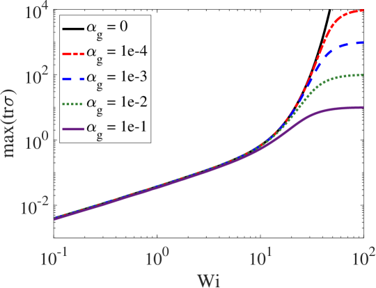
Figure 12: Numerical solution of $\max({\rm tr}\;\boldsymbol{\sigma})$ as a function of Wi at $\textrm{De}=1,$ for a range of $0\leq\alpha_{g}\leq 0.1,$ at a given oscillatory extensional stagnation point in the Giesekus model.

References

- [1] Ricardo Cortez. The method of regularized stokeslets. SIAM Journal on Scientific Computing, 23(4):1204–1225, 2001.
- [2] JM Dealy. Weissenberg and Deborah numbers: Their definition and use. Rheol. Bull, 79(2):14–18, 2010.
- [3] Gwynn J Elfring and Gaurav Goyal. The effect of gait on swimming in viscoelastic fluids. Journal of Non-Newtonian Fluid Mechanics, 234:8–14, 2016.
- [4] Henry C Fu, Thomas R Powers, and Charles W Wolgemuth. Theory of swimming filaments in viscoelastic media. Physical review letters, 99(25):258101, 2007.
- [5] Henry C Fu, Charles W Wolgemuth, and Thomas R Powers. Beating patterns of filaments in viscoelastic fluids. Physical Review E, 78(4):041913, 2008.
- [6] Henry C Fu, Charles W Wolgemuth, and Thomas R Powers. Swimming speeds of filaments in nonlinearly viscoelastic fluids. Physics of Fluids (1994-present), 21(3):033102, 2009.
- [7] Hanswalter Giesekus. A simple constitutive equation for polymer fluids based on the concept of deformation-dependent tensorial mobility. Journal of Non-Newtonian Fluid Mechanics, 11(1-2):69–109, 1982.
- [8] Christopher John Guido, Jeremy P Binagia, and Eric SG Shaqfeh. Three-dimensional simulations of undulatory and amoeboid swimmers in viscoelastic fluids. Soft Matter, 2019.
- [9] Robert D Guy and Becca Thomases. Computational challenges for simulating strongly elastic flows in biology. In Complex fluids in biological systems, pages 359–397. Springer, 2015.
- [10] Eric Lauga. Propulsion in a viscoelastic fluid. Phys. Fluids, 19(8):83104, 2007.
- [11] Chuanbin Li. A Numerical Study on Flagellar Swimming in Viscoelastic Fluids Based on Experimental Data. University of California, Davis, 2017.
- [12] Chuanbin Li, Boyang Qin, Arvind Gopinath, Paulo E Arratia, Becca Thomases, and Robert D Guy. Flagellar swimming in viscoelastic fluids: role of fluid elastic stress revealed by simulations based on experimental data. Journal of The Royal Society Interface, 14(135):20170289, 2017.
- [13] Chuanbin Li, Becca Thomases, and Robert D Guy. Orientation dependent elastic stress concentration at tips of slender objects translating in viscoelastic fluids. Physical Review Fluids, 4(3):031301, 2019.
- [14] Charles S Peskin. The immersed boundary method. Acta numerica, 11:479–517, 2002.
- [15] Robert Poole. The deborah and Weissenberg numbers. The British Society of Rheology - Rheology Bulletin, 53:32–39, 06 2012.
- [16] Emily E Riley and Eric Lauga. Enhanced active swimming in viscoelastic fluids. EPL (Europhysics Letters), 108(3):34003, 2014.
- [17] Daniel Salazar, Alexandre M. Roma, and Hector D. Ceniceros. Numerical study of an inextensible, finite swimmer in stokesian viscoelastic flow. Physics of Fluids, 28(6):063101, 2016.
- [18] Saverio E Spagnolie, Bin Liu, and Thomas R Powers. Locomotion of helical bodies in viscoelastic fluids: enhanced swimming at large helical amplitudes. Physical review letters, 111(6):068101, 2013.
- [19] R Sureshkumar and Antony N Beris. Effect of artificial stress diffusivity on the stability of numerical calculations and the flow dynamics of time-dependent viscoelastic flows. Journal of Non-Newtonian Fluid Mechanics, 60(1):53–80, 1995.
- [20] Joseph Teran, Lisa Fauci, and Michael Shelley. Viscoelastic fluid response can increase the speed and efficiency of a free swimmer. Physical review letters, 104(3):038101, 2010.
- [21] Becca Thomases. An analysis of the effect of stress diffusion on the dynamics of creeping viscoelastic flow. Journal of Non-Newtonian Fluid Mechanics, 166(21):1221–1228, 2011.
- [22] Becca Thomases and Robert D Guy. Mechanisms of elastic enhancement and hindrance for finite-length undulatory swimmers in viscoelastic fluids. Physical review letters, 113(9):098102, 2014.
- [23] Becca Thomases and Robert D Guy. The role of body flexibility in stroke enhancements for finite-length undulatory swimmers in viscoelastic fluids. Journal of Fluid Mechanics, 825:109–132, 2017.
- [24] Becca Thomases and Robert D Guy. The role of body flexibility in stroke enhancements for finite-length undulatory swimmers in viscoelastic fluids. Journal of Fluid Mechanics, 2017. In Press.
- [25] Becca Thomases and Michael Shelley. Emergence of singular structures in Oldroyd-B fluids. Physics of fluids, 19(10):103103, 2007.