Identifying Effective Scenarios for Sample Average Approximation

ABSTRACT 

We introduce a method to improve the tractability of the well-known Sample Average Approximation (SAA) without compromising important theoretical properties, such as convergence in probability and the consistency of an independent and identically distributed (iid) sample. We consider each scenario as a polyhedron of the mix of first-stage and second-stage decision variables. According to John’s theorem, the Löwner-John ellipsoid of each polyhedron will be unique which means that different scenarios will have correspondingly different Löwner-John ellipsoids. By optimizing the objective function regarding both feasible regions of the polyhedron and its unique Löwner-John ellipsoid, respectively, we obtain a pair of optimal values, which would be a coordinate on a two-dimensional plane. The scenarios, whose coordinates are close enough on the plane, will be treated as one scenario; thus our method reduces the sample size of an iid sample considerably. Instead of using a large iid sample directly, we would use the cluster of low-cost computers to calculate the coordinates of a massive number of scenarios and build a representative and significantly smaller sample to feed the solver. We show that our method will obtain the optimal solution of a very large sample without compromising the solution quality. Furthermore, our method would be implementable as a distributed computational infrastructure with many but low-cost computers.

KEYWORDS: Sample Average Approximation, Löwner-John Ellipsoid, Stochastic Programming 
HISTORY: This paper was first submitted on March 21, 2019.

1 Introduction

A standard formulation of the two-stage stochastic program is

$$\min_{x}\{c^{T}x+\mathbb{E}[Q(x,\xi)],x\in X\subset\mathbb{R}^{n}\}$$ (1)

where

$$Q(x,\xi):=\inf_{y}\{q^{T}y:Wy\geq h-Tx,y\in Y\subset\mathbb{R}^{m}\}$$

and $\xi$ represents a random vector whose distribution has finite support. $W$ is a deterministic matrix, while $h$ and $T$ would be functions with respect to $\xi$. If $X\subset\mathbb{Z}^{n},$ and $Y\subset\mathbb{Z}^{m}$, the problem becomes a stochastic integer program.

A common practice to numerically solve stochastic (integer) program is by sampling. In [9], the authors generate iid realizations, $\xi^{1},\ldots,\xi^{N}$, of the random vector $\xi$ and approximate the objective function $\mathbb{E}[Q(x,\xi)]$ with its average $\dfrac{1}{N}\sum_{i=1}^{N}Q(x,\xi^{i})$. The stochastic (integer) program becomes a deterministic model as follows:

$$\min_{x}\{c^{T}x+\dfrac{1}{N}\sum_{i=1}^{N}Q(x,\xi^{i}),x\in X\}$$ (2)

Let $\hat{\nu}_{N}$ and $\hat{x}_{N}$ denote the optimal value and the optimal solution of (2), respectively while $\nu^{*}$ and $x^{*}$ represent the optimal value and the optimal solution of (1). The authors showed that both $\hat{\nu}_{N}$ and $\hat{x}_{N}$ will converge to their counterparts as the sample size $N$ becomes large enough, regardless of the distribution of $\xi$. These results are referred to as convergence in probability and consistency. This method is referred to as the Sample Average Approximation (SAA) and in [5], we have the convergence results regarding a few sampling methods. We find the recent advance of SAA in [6] and [12] with references therein.

The computational cost is entirely determined by the sample size $N$. The theoretical argument in determining the sample size $N$ is based on the Large Deviation theory (see [13]). According to this theory, there is a high probability that the values of the sample average approximation and the true function are close to each other at a sufficiently dense set of points. The result is impractical because the required sample size has been one of the primary impediments to SAA’s implementation in practice. Moreover, in [4], the stochastic program is recognized as #P-hard, which indicates that it is computationally intractable. The term #P-hard, rather than NP-hard, is used to describe the fact that the computer hardware will be overwhelmed by the number of scenarios required to complete the numerical method. For the stochastic integer program, it becomes worse because a large sample size will lead to an unrealistically large deterministic integer program.

Efforts to reduce the sample size may introduce the SAA method to many scenario-rich industries, such as financial planning and logistics. There are a few major ideas: the scenario reduction method, such as [3], the variance reduction method in [15], and the Quasi-Monte-Carlo method in [10]. There are many articles prior to the papers mentioned above. In [8], the authors present a comprehensive review on the SAA, such that a moderately large sample is more likely to be satisfactory for some problems. Thus, when a practitioner encounters a stochastic (integer) program, the choice would be either to hope for a moderately large sample that will deliver a satisfactory numerical solution, or to adopt the reduction methods or the Quasi-Monte-Carlo method with non-iid samples.

The SAA method with a moderately large sample could be either satisfactory or otherwise because the sample size requirement imposed by the Large Deviation theory will never be met in practice. The obtained solution may still converge to the true optimal solution, while the variation of the obtained optimal value could be concerning. A viable solution to reducing the variation of the optimal solution is to increase the sample size of the iid sample, which will lead to intractability. Reduction methods, such as scenario reduction, variance reduction, and the Quasi-Monte-Carlo, aim to sample the random variable in an artificially defined manner. These methods will effectively reduce the sample size and assure tractability. However, since the scenarios of these methods are no longer independently generated, the obtained optimal solution may exhibit, at least theoretically, bias with respect to the true optimal solution and the distribution of the sample average will no longer be normal. Therefore, the situation is that if we use the SAA method, we may have a computationally challenging optimization problem, while we may incur an inconsistent optimal solution when adopting the reduction methods.

In this paper, we study a method to preserve the convergence in probability, the consistency regarding the optimal solution and to control computational tractability. The idea is to first generate a large enough Independent and Identically Distributed (iid) sample. Instead of using this large iid sample directly, we will attach values to each sampled scenario as a measure of similarity, and we will cluster “similar” scenarios as a representative scenario with an adjusted probability to formulate a new, but reduced sample. We show that the newly formed sample will yield a consistent optimal solution with a bounded difference to the counterpart of the original large iid sample.

The essential result is to define the measure of similarity. We realize that each scenario is described as a polyhedron if not empty. To measure the similarity of polyhedrons of the same dimension, we need to compare them as distinct geometric objects, which is difficult due to the exploding number of vertices. We have to transform polyhedrons into comparable geometric objects, and the most well-known object is the Löwner-John ellipsoid, which is the maximum volume inscribed ellipsoid that is contained in the polyhedron. The Löwner-John ellipsoid is unique to each convex body ([7]). In other words, the mapping from the polyhedron to its Löwner-John ellipsoid is a one-to-one correspondence. For the same objective function regarding different feasible regions such as the polyhedron and its Löwner-John ellipsoid, the pair optimal values would be considered as a coordinate on a two-dimensional plane. We define the similar scenarios as the scenarios whose coordinates stay close and our method will identify similar scenarios and consolidate them as one representative scenario to achieve the goal of reducing the sample size.

Our method is both theoretically and computationally plausible. The Löwner-John ellipsoid is a good choice when approximating polyhedrons of distinct scenarios because the mapping from the polyhedron to its Löwner-John ellipsoid is a one-to-one correspondence. We realize that distinct scenarios will have distinct Löwner-John ellipsoids, which are strictly convex. When the objective function is convex and we use the Löwner-John ellipsoid as the feasible region, the optimal values associated with distinct ellipsoids will be distinct as well. We also obtain the optimal values of the same objective function subject to the polyhedron as feasible region. Thus, we can scalarize distinct scenarios into distinct pairs of coordinates and the seemingly different geometric objectives become comparable as the coordinates on a two-dimensional plane.

The efficient computational methods of Löwner-John ellipsoids are available; see [14] for more details. There are multiple software packages, such as SeDuMi and SDPA, which are ready for implementations. Furthermore, since our method will evaluate the similarity of each scenario, it can be implemented on multiple, low-cost computers deployed in parallel to process a large iid sample. The benefit of our method is to reduce the problem scale to its fractions to improve the tractability of SAA of large sample. The remainder of the paper is organized as follows. We present the connection between a sampled scenario and an ellipsoid in Section 2. In Section 3, we show the computation of the measure of similarity among distinct scenarios, followed by details regarding the clustering method, along with the result of preserving of convergence in probability and consistency of the SAA in Section 4. In Section 5, we present multiple examples to show the numerical results, and we conclude our research in Section 6.

2 Löwner-John ellipsoid associated with each scenario

In this section, we present the approximation of a scenario using the Löwner-John ellipsoid. Suppose that we have a two-stage stochastic (integer) programming. The distribution of $\xi$ would be either continuous or discrete in terms of finite support. Additionally, there would be finitely or infinitely many realizations. The problem is solved by the SAA with a sample size $K$, i.e., $\xi^{1},\ldots,\xi^{k},\ldots,\xi^{K}$ are $K$ realized scenarios:

$$\min_{x}\{c^{\prime}x+\dfrac{1}{K}\sum_{k=1}^{K}Q(x,\xi^{k})]|Ax\leq b,x\geq 0\}$$

and

$$Q(x,\xi^{k})=\min_{y}\{q_{k}^{\prime}y|Wy\leq h_{k}-T_{k}x,y\geq 0\}$$

where the matrices $q_{k},T_{k},h_{k}\in\mathbb{R}^{m}$ would be functions of $\xi$, and $W$ is a fixed $\ell\times m$ matrix. $Q(x,\xi)$ refers to the recourse function.

We assume that when the first-stage decisions are discrete, the set of first-stage decisions is finite and non-empty. Also, the recourse function $Q(x,\xi)$ is measurable and both $\mathbb{E}[Q(x,\xi)]$ and $\mathbb{E}[Q^{2}(x,\xi)]$ are finite for every feasible $x$. Otherwise, i.e., if the first-stage decisions are continuous, the set of first-stage decisions is non-empty, compact, and polyhedral. Also, the recourse function $Q(x,\xi^{k})$ is finite for $k=1,\ldots,K$. In addition, we assume that for any first-stage decision, the feasible set of the recourse variable $y$ is non-empty and finite.

The SAA method solves the following deterministic optimization problem.

$$\min_{x,y_{1},\ldots,y_{K}} \ c^{\prime}x+\dfrac{1}{K}\sum_{k=1}^{K}q_{k}^{\prime}y_{k}$$

subject to $$\ Ax\leq b,x\geq 0,x\in X\subset\mathbb{R}^{n}$$ (3)

$$\ Wy_{k}\leq h_{k}-T_{k}x,y_{k}\geq 0,k=1,\ldots,K.$$

and the first-stage optimal solution is $x_{K}^{*}$ with the optimal value $\nu^{*}_{K}$. We are interested in the case of only one scenario, $\xi^{k},k\in\{1,\ldots,K\}$, which is selected. We have

$$\kappa(k):=\min_{x_{k},y_{k}} \ c^{\prime}x_{k}+q_{k}^{\prime}y_{k}$$

subject to $$\ Ax_{k}\leq b,x_{k}\geq 0,x_{k}\in X\subset\mathbb{R}^{n}$$ (4)

$$\ Wy_{k}\leq h_{k}-T_{k}x_{k},y_{k}\geq 0.$$

where $x_{k}$ and $y_{k}$ are the first-stage and second-stage decisions, respectively. We define that for a non-empty and bounded sampled scenario $\xi^{k}$,

Definition 1.

$$P_{k}:=\{[x_{k};y_{k}]|Wy_{k}\leq h_{k}-T_{k}x_{k},y_{k}\geq 0\}$$ (5)

is the $(n+m)$ dimensional scenario polyhedron of the scenario $\xi_{k}$.

We note that if the decisions are integers, i.e., $x_{k},y_{k}\in\mathbb{Z}^{n+m}$, we need to relax the integer constraints to $x_{k},y_{k}\in\mathbb{R}^{n+m}$ to assure that $P_{k}$ a non-empty and bounded polyhedron.

Definition 2.

An ellipsoid $E$ of $\mathbb{R}^{n+m}$ is an affine image of the unit ball $B_{n+m}:=\{u\in\mathbb{R}^{n+m}:||u||\leq 1\}$, that is

$$E:=\{c+Su:u\in\mathbb{R}^{n+m},||u||\leq 1\},\textrm{or }E:=\{x\in\mathbb{R}^{n+m}:||S^{-1}(x-c)||\leq 1\}$$

where $S\in\mathbb{R}^{(n+m)\times(n+m)}$ is a symmetric, non-singular, and positive definite matrix.

Also, we need the following assumption.

Assumption 1.

$P_{k}$ satisfies the Slater’s condition.

This assumption is rather important because otherwise, a bounded and non-empty $P_{k}$ could be a degenerate polyhedron, which has zero volume for Löwner-John ellipsoid. More importantly, many two-stage stochastic programming has equality constraints in the second stage. For example, in the aircraft allocation problem in [2], the second stage is constructed with equality constraints and the Löwner-John ellipsoid will degenerate. Consider the equality constraint

$$Wy_{k}=h_{k}-T_{k}x,y_{k}\geq 0,k\in\{1,\ldots,K\}$$ (6)

To satisfy the slater’s condition, we replace the constraints (6) by the following

$$Wy_{k}\leq h_{k}-T_{k}x+\epsilon\mathbf{1},-Wy_{k}\leq T_{k}x-h_{k}+\epsilon\mathbf{1},y_{k}\geq 0,k\in\{1,\ldots,K\}$$ (7)

where $\mathbf{1}\in\mathbb{R}^{\ell}$ with all the components are valued 1 and $\epsilon>0$ is a small enough value.

We now present the well-known John’s theorem.

Theorem 1.

Let $C$ be a non-empty and bounded polyhedron, which satisfies the Slater’s condition, in $\mathbb{R}^{n+m}$. There exists a unique ellipsoid, the Löwner-John ellipsoid, which is the smaximum value inscribed ellipsoid of C.

We find the proof of Theorem 1 in many articles, e.g., [1]. For each $P_{k}$, we use $(S(k),c(k))$ to represent the Löwner-John ellipsoid, where $c(k)$ is the center of the ellipsoid, and $S(k)$ is the symmetric positive definite matrix. The calculation of Löwner-John ellipsoid is to solve a semi-definite program, which is a convex optimization problem. The objective function is to minimize the logarithmic function of the determinant of $S^{-1}(k)$. The computational complexity is $O[(n+m)^{3}]$ (see [1]), which indicates the availability of efficient solution methods. For $P_{k}$, we have

$$(S(k),c(k))\subset P_{k}\in\mathbb{R}^{n+m}$$ (8)

and $(S(k),c(k))$ is unique to $P_{k}$ because Theorem 1 proves that the mapping from each $P_{k}$ to $(S(k),c(k))$ is a one-to-one correspondence.

3 Measuring similarity

We now construct a measure of similarity among distinct $P_{k},k=1,\ldots,K$. Consider two distinct scenario polyhedrons, $P_{j}$ and $P_{k}$, such that $j,k\in\{1,\ldots,K\}$ and $j\neq k$. $P_{j}$’s Löwner-John ellipsoid is $(S(j),c(j))$ and $(S(k),c(k))$ is $P_{k}$’s Löwner-John ellipsoid. We define

$$\sigma(k):=\min_{x_{k},y_{k}}\{c^{\prime}x_{k}+q^{\prime}_{k}y_{k}:[x_{k};y_{k}]\in(S(k),c(k)),x_{k},y_{k}\geq 0\}$$ (9)

and its optimal solution is $[x_{k}^{*};y_{k}^{*}]$. By the feasible region argument, we have

$$-\infty\leq\kappa(k)\leq\sigma(k)\leq\infty$$ (10)

$\sigma(k),\textrm{ and }\kappa(k),k=1,\ldots,K$ would be easily calculated. We also assume

Assumption 2.

There exists a value $\mathbb{D}<\infty$ that $|\sigma(k)-\kappa(k)|\leq\mathbb{D},k=1,\ldots,K$.

The measure of similarity involving the scenario $\xi^{k}$ would be $(\kappa(k),\sigma(k))$. Such a poll of coordinates ($k=1,\ldots,K$) formulates a scatter plot. By using a fine grid setting, we would be able to choose representative scenarios. According to Theorem 1, the mapping from $P_{k}$ to $(S(k),c(k))$ would be the one-to-one correspondence, which means that although comparing $\xi^{j}$ and $\xi^{k}$ are difficult, the comparison becomes between two Löwner-John ellipsoids, $(S(k),c(k))$ and $(S(j),c(j))$. Since Löwner-John ellipsoid feasible region is strictly convex, both optimal solutions $[x_{k}^{*};y_{k}^{*}]$ and $[x_{j}^{*};y_{j}^{*}]$ and optimal values $\sigma(k)$ and $\sigma(j)$ are unique. Thus, two distinct scenarios $\xi^{k}$ and $\xi^{j}$ are equivalently converted to two distinct optimal values $\sigma(k)$ and $\sigma(j)$, respectively. We scalarize the non-comparable scenarios to comparable real values.

For any feasible first-stage decision $x_{0}$, we have

$$Q(x_{0},\xi^{k}):=\min\{q_{k}^{\prime}y:[x_{0};y]\in P_{k}\}$$ (recourse value)

and it is true that $\kappa(k)\leq Q(x_{0},\xi^{k})$ for any $x_{0}$. According to (10), we need both $\sigma(k)$ and $\kappa(k)$ to bound the recourse value of any first-stage decision from both sides. Thus, we use the coordinate $(\kappa(k),\sigma(k))$ as the similarity measure.

The similarity measure $(\kappa(k),\sigma(k))$ will help remove stage dependency. In other words, when solving the stochastic program using the SAA, all sampled $K$ scenarios must share the same first-stage decision. We have a dilemma, in that we need to quantify the similarity of $K$ iid scenarios involving the same first-stage decision, while the stochastic program needs to find the first-stage decision in order to optimize the objective. We need a similarity measure, which is consistent to any first-stage decisions. By using the coordinate $(\kappa(k),\sigma(k))$, for any first-stage decision $x\in X$, we have

$$\kappa(k)\leq Q(x,\xi^{k})\leq\sigma(k)$$

where $k=1,\ldots,K$. $(\kappa(k),\sigma(k))$ serves as a spectrum, and regardless of the first-stage decision, the recourse value will be well positioned within the spectrum. We define that for each $x\in X$,

$$\epsilon_{k}(x):=\sigma(k)-Q(x,\xi^{k})\geq 0$$ (11)

and for each pair of distinct scenarios $j$ and $k$, with Assumption 2, we have, for any $x\in X$,

$$|\epsilon_{j}(x)-\epsilon_{k}(x)|\leq\mathbb{D}$$ (12)

Consider two distinct scenarios, which could be significantly different in many geometric aspects. However, the recourse value under $\xi^{k}$ of any first-stage decision $x$, $Q(x,\xi^{k})$, shares unique upper and lower bounds associated with the scenario $\xi^{k}$. Regarding the practice of the SAA, when two seemingly distinct scenarios’ recourse values $Q(x,\xi^{k})$ and $Q(x,\xi^{k})$ share the similar upper and lower bounds, these two scenarios will yield similar impact to the sample average $\dfrac{1}{K}\sum_{k=1}^{K}Q(x,\xi^{k})$ and therefore they may be possibly considered as similar. In other words, we reduce the iid sample size by clustering similar scenarios, quantified by the spectrum of the recourse value. We show in the next section that our clustering method will preserve the convergence in probability and consistency results of the SAA.

4 Clustering similar scenarios

4.1 Preserving convergence rate and consistency

Consider the SAA problem with a sample of size $K$, $\xi^{1},\ldots,\xi^{K}$,

$$\min_{x} \ c^{\prime}x+\dfrac{1}{K}\sum_{k=1}^{K}Q(x,\xi^{k})$$

subject to $$\ Ax\leq b,x\geq 0,x\in X\subset\mathbb{R}^{n}$$ (13)

with the optimal solution $x_{K}^{*}$ and the optimal value $\nu_{K}^{*}:=\nu_{K}(x_{K}^{*})$. Consider two similar scenarios $\xi^{j}$ and $\xi^{k}$, such that $|\kappa(j)-\kappa(k)|\leq\dfrac{\delta}{2}$ and $|\sigma(j)-\sigma(k)|\leq\dfrac{\delta}{2}$ for a $\delta>0$. We cluster scenario $j$ with scenario $k$. After clustering, the iid sample $\xi^{1},\ldots,\xi^{K}$ becomes $\xi^{1},\ldots,\xi^{j-1},\xi^{k},\xi^{j+1},\ldots,\xi^{K}$ with the probability $\dfrac{1}{K}$. That is, scenario $\xi^{k}$ has a probability of $\dfrac{2}{K}$ because we replace $\xi^{j}$ with $\xi^{k}$. We have:

$$\min_{x} \ c^{\prime}x+\dfrac{1}{K}[\sum_{k\neq j}^{K}\bigg{(}\sigma(k)-\epsilon_{k}(x)\bigg{)}+\sigma(k)-\epsilon_{j}(k)]$$

subject to $$\ Ax\leq b,x\geq 0,x\in X\subset\mathbb{R}^{n}$$ (14)

The difference between the objectives of (4.1) and (4.1) at $x$ is bounded by

$$\dfrac{1}{K}\bigg{|}\sigma(j)-\sigma(k)+\epsilon_{k}(x)-\epsilon_{j}(x)\bigg{|}\leq\dfrac{\delta}{2K}+\dfrac{\mathbb{D}}{2K}.$$ (15)

For a $\delta>0$, we cluster a certain number of scenarios, $K(\delta)$. There are $K-K(\delta)$ scenarios left for the SAA. Let $\mathcal{J}$ represent the set of indices of the scenarios being clustered, and let $\mathcal{K}$ represent the set of indices of the scenarios remaining in the model. We refer to scenarios in $\mathcal{K}$ as the representative scenarios. The optimal solution is $\tilde{x}_{K}^{*}$, and the optimal value becomes $\tilde{\nu}_{K}^{*}:=\tilde{\nu}(\tilde{x}_{K}^{*})$. We use $\tilde{\nu}_{K}(x)$ to represent the objective function of the reduced sample. The value of $|\tilde{\nu}_{K}(x)-\nu_{K}(x)|$ is the measure of the solution quality in comparison to the SAA.

$$|\tilde{\nu}_{K}(x)-\nu_{K}(x)|\leq\dfrac{\delta K(\delta)}{2K}+\dfrac{K(\delta)\mathbb{D}}{2K}$$ (16)

The goal of our clustering approach is to reduce the sample size of an iid sample and to preserve the consistency and convergence in probability of the SAA.

Theorem 2.

For an iid sample of size $K$, we cluster $K(\delta)$ times, then,

$$|\tilde{\nu}_{K}^{*}-\nu_{K}^{*}|\rightarrow 0$$ (17)

as $K\rightarrow\infty$ with probability 1.

Proof.

By definition, we have

$$\tilde{\nu}_{K}(\tilde{x}_{K}^{*})\leq\tilde{\nu}_{K}(x_{K}^{*})\textrm{ and }\nu_{K}(x_{K}^{*})\leq\nu_{K}(\tilde{x}_{K}^{*})$$ (18)

By (16), when $K$ is large enough, and for any $\epsilon>0$, we have

$$\tilde{\nu}_{K}(\tilde{x}_{K}^{*})\leq\tilde{\nu}_{K}(x_{K}^{*})\leq\nu_{K}(x_{K}^{*})+\epsilon\textrm{ and }\nu_{K}(x_{K}^{*})\leq\nu_{K}(\tilde{x}_{K}^{*})\leq\tilde{\nu}_{K}(\tilde{x}_{K}^{*})+\epsilon$$

Both $\tilde{\nu}_{K}(x)$ and $\nu_{K}(x)$ are convex function with respect to $x$, and when $K$ is large enough, we have $|\tilde{\nu}^{*}_{K}-\nu_{K}^{*}|\leq\epsilon$ with probability 1. ∎

There is another appearance of the above result: for a sample size of $K$, we cluster up to $K(\delta)$ times, and we have

$$\lim_{K\rightarrow\infty}\mathbb{P}(|\tilde{\nu}_{K}^{*}-\nu_{K}^{*}|>\epsilon)=0$$

We complete the analysis regarding the consistency of the SAA.

We now present the impact of our clustering method on the convergence in probability of the SAA. The clustering method will reduce the original sample size $K$ to its fraction. Let $\mathcal{S}_{K}^{\epsilon}$ and $\mathcal{S}^{\epsilon}$ be the sets of the $\epsilon$-optimal solutions of the SAA and the original problems, respectively. Both $\mathcal{S}_{K}^{\epsilon}$ and $\mathcal{S}^{\epsilon}$ are non-empty and finite for any $\epsilon>0$. Let $\mathcal{S}$ represent the set of optimal solutions of the original problem. When pursuing different accuracy in the SAA and the original problem with an accuracy of $\gamma>0$ and an $\epsilon>0$, respectively, such that $\gamma\leq\epsilon$, the event $\{\mathcal{S}_{K}^{\gamma}\subset\mathcal{S}^{\epsilon}\}$ means that the solution of the SAA provides an $\epsilon$-optimal solution for the original problem. We need the following definition and assumption.

Definition 3.

Let $X:=\{x|Ax\leq b,x\geq 0\}$. $u(x)$ is a mapping from $X\backslash\mathcal{S}^{\epsilon}$ into the set $\mathcal{S}$, in which $u(x)\in\mathcal{S}$ for all $x\in X\backslash\mathcal{S}^{\epsilon}$, such that for $\epsilon^{*}:=\min_{X\backslash\mathcal{S}^{\epsilon}}\nu(x)-\nu^{*}$, $\epsilon^{*}\geq\epsilon$,

$$\nu(u(x))\leq\nu(x)-\epsilon^{*}\textrm{ for all }x\in X\backslash\mathcal{S}^{\epsilon}$$

Assumption 3.

For every $x\in X\backslash\mathcal{S}^{\epsilon}$, the moment-generating function of the random variable $Y(x,\xi):=c^{\prime}u(x)+Q(u(x),\xi)-c^{\prime}u-Q(x,\xi)$ is finite valued in a neighborhood of $t=0$.

We thus have the following result, whose proof is in [13].

Theorem 3.

Let $\epsilon$ and $\gamma$ be non-negative numbers, such that $\gamma\;eq\epsilon$. Then

$$1-\mathbb{P}(\mathcal{S_{K}^{\gamma}}\subset\mathcal{S}^{\epsilon})\leq Me^{-K\eta(\gamma,\epsilon)}$$ (19)

where $\eta(\gamma,\epsilon):=\min_{x\in X\backslash\mathcal{S}^{\epsilon}}\mathcal{I}_{x}(-\gamma)$ and $\mathcal{I}_{x}(\cdot)$ denote the rate function of the random variable $Y(x,\xi)$. With Assumption 3, $\eta(\gamma,\epsilon)>0$, and $M$ is the number of scenarios of the original problem.

After clustering the scenarios, the reduced sample is no longer iid, and we need Theorem 3 to obtain the new convergence rate results. Let $\beta:=\dfrac{K(\delta)\delta}{2K}+\dfrac{K(\delta)\mathbb{D}}{2K}$ be the error bound of the clustering $K(\delta)$ scenarios, and we solve the SAA model for a $\tau$-optimal solution. We denote $\mathcal{S}_{K,\delta}^{\tau,\beta}$ as the set of resulting optimal solution, such that $\mathcal{S}_{K,\delta}^{\tau,\beta}\subset\mathcal{S}_{K}^{\gamma}$. We have

Theorem 4.

For an iid sample of size $K$ and $\delta>0$, we cluster $K(\delta)$ scenarios with the error bound $\beta$, and we solve the SAA with a reduced sample and with an accuracy of $\tau$. If $\mathcal{S}_{K,\delta}^{\tau,\beta}\subset\mathcal{S}_{K}^{\gamma}$ is true, then

$$\lim_{K\rightarrow\infty}\sup\dfrac{1}{K}\log\bigg{[}1-\mathbb{P}(\mathcal{S}_{K,\delta}^{\tau,\beta}\subset\mathcal{S}^{\epsilon})\bigg{]}\leq-\eta({\gamma,\epsilon})$$ (20)

Proof.

Since $\mathcal{S}_{K,\delta}^{\tau,\beta}\subset\mathcal{S}_{K}^{\gamma}$, we have

$$\mathbb{P}(\mathcal{S}_{K,\delta}^{\tau,\beta}\subset\mathcal{S}^{\epsilon})\geq\mathbb{P}(\mathcal{S}_{K}^{\gamma}\subset\mathcal{S}^{\epsilon})$$ (21)

and we apply Theorem 4,

$$1-\mathbb{P}(\mathcal{S}_{K,\delta}^{\tau,\beta}\subset\mathcal{S}^{\epsilon})\leq Me^{-K\eta(\gamma,\epsilon)}.$$ (22)

Applying (20) and (22), we reach the result. ∎

We note that the above result is developed for the stochastic program, which relaxes the integer constraints, if necessary. Because all of the feasible sets are bounded, non-empty, and non-degenerate, we can use similar arguments to draw conclusions regarding the convergence in probability and consistency for stochastic integer programs. We now present the clustering approach by steps.

1. Generate a large enough iid sample of size $K$. By relaxing the integer variables, if necessary, we have $K$ scenario polyhedrons.

2. Calculate the Löwner-John Ellipsoid for each scenario polyhedron.

3. Calculate $\sigma(k)$, and $\kappa(k),k=1,\ldots,K$ for each scenario polyhedron.

4. Determine the value of $\delta$, which will result in $K(\delta)$ scenarios removed from the original sample. The choice of $\delta$ would be problem-dependent.

5. Cluster all scenarios, such that $|\sigma(k)-\sigma(j)|\leq\dfrac{\delta}{2}$ and $|\kappa(k)-\kappa(j)|\leq\dfrac{\delta}{2}$, and replace them with one representative scenario $\xi^{k},k\in\mathcal{K}$.

6. Solve the SAA with the reduced sample.

The above method performs very well regarding solution quality for the problems in Section 5. In the next subsection, we present the connection between our method with the other sampling methods. Basically, our method and other sampling methods share the same goal to solve the tractability issue.

4.2 Connection with other sampling methods

Our method of clustering scenarios are well connected with other sampling methods surveyed in [6] that all sampling methods, including our clustering method in this paper, would reduce the sample size for better tractability and high-quality solution. The SAA method solves a deterministic optimization problem as the approximate to the original stochastic programming. The SAA method using iid samples has an advantage over other non-iid sampling methods that it simplifies the underlying mathematics of many statistical method and it assures $\dfrac{1}{K}\sum_{k=1}^{K}Q(x,\xi^{k})$ to follow a normal distribution. The SAA method using iid samples also has nice theoretical results such as convergence in probability and consistency. However, the required sample size may be overwhelmingly large and the scale of the resulting deterministic optimization problem may easily be out of control. Thus, the non-iid sampling methods are developed to find good approximations to the original distribution while not raising the tractability issue.

Most sampling methods work on the distribution side that the researchers attempt to find a good replacement to the original distribution. If the goal is achieved, the non-iid sample will be used to calculate $\dfrac{1}{K}\sum_{k=1}^{K}Q(x,\xi^{k})$. Our method, however, focuses directly on the value of the recourse function of any first-stage decision, $Q(x,\xi^{k})$. Instead of finding a good replacement to the original distribution, we will sample the scenarios which lead to representative values of $Q(x,\xi^{k})$, which are bounded by the coordinates. Thus, the difference between our method and other non-iid sampling method is that our method is a recourse-value-oriented method.

Such a difference will disappear in a newsvendor problem as follows.

Example 1.

Consider a seller that must choose the amount $x$ of inventory to obtain at the beginning of a selling season. The decision is made only once, i.e., there is no opportunity to replenish inventory during the selling season. The demand $\xi$ during the selling season is a nonnegative random variable with cumulative distribution function $F$. The cost of obtaining inventory is $c$ per unit. The product is sold at a given price $r$ per unit during the selling season, and at the end of the season unsold inventory has a salvage value of $v$ per unit. The seller wants to choose the amount $x$ of inventory that solves

$$\min_{x}\ \{g(x)=\mathbb{E}[cx-r\min\{x,\xi\}-v\max\{x-\xi,0\}]\}$$ (23)

If we present the newsvendor problem in the form of two-stage stochastic programming, we have

$$\min_{x}\ cx+\mathbb{E}[Q(x,\xi)]$$

$$\textrm{where}\ Q(x,\xi):=\min_{y^{+},y^{-}}\{(r-c)y^{-}+(c-v)y^{+}|x-y^{+}+y^{-}=\xi,y^{+},y^{-}\geq 0\}$$

For a scenario $\xi^{k}$, our method will have the following model as a start.

$$\kappa(k):=\min_{x,y^{+},y^{-}}\{cx+(r-c)y^{-}+(c-v)y^{+},x-y^{+}+y^{-}=\xi^{k},y^{+},y^{-}\geq 0\}$$ (24)

For this problem, the Löwner-John ellipsoid degenerates and $\sigma(k)=0$ and $\kappa(k)=cx^{k}$. The optimal solution is $x^{k}=\xi^{k}$ for (24) and the coordinate becomes $(0,cx^{k})=(0,c\xi^{k})$. Thus, our clustering method will consolidate similar scenarios $\xi^{k}$ and $\xi^{j},j\neq k$, such that $|c\xi^{k}-c\xi^{j}|\leq\dfrac{\delta}{2}$. We now realize that for the newsvendor problem, our clustering method behaves just like other sampling methods such as the importance sampling and the Quasi-Monte Carlo method to work on the distribution side. This example shows that our method shares the same goal as other sampling methods, which is to approximate the value of $\dfrac{1}{K}\sum_{k=1}^{K}Q(x,\xi^{k})$. Our clustering method works on a large iid sample for the sake of preserving the nice theoretical results and then reduces the sample size by focusing on the recourse-value at any first-stage decision rather than the original distribution.

We present a cost-benefit discussion for our clustering method with respect to the stochastic program, in particular, the stochastic integer program. For an iid sample of size $K$, the cost involves solving the $K$ Semi-Definite Programs (SDP) in order to calculate the Löwner-John Ellipsoids. Thanks to the advance of convex optimization, the cost is less of a concern because the SDP can be solved very quickly and efficiently. Also, the clustering method can highlight the scenarios, which greatly impact the recourse value, rather than treating every scenario evenly. Decision-makers may be more interested in identifying several scenarios that deserve more attention.

The benefit of our approach is that we greatly reduce the number of scenarios without compromising solution quality. A reduction in the scenarios implies a reduction in the number of decision variables and constraints. In the following section, we demonstrate that the clustering method reduces an integer program of 202 integer variables and 201 integer constraints to another instance of 20 integer variables and 19 integer constraints. Consider the fact that when the removed decision variables are integers, the benefit of reducing the problem to its fraction can be easily justified. In real-world implementation, practitioners can start clustering scenarios at an early time in order to “select” scenarios from a iid sample of massive scenarios. Once a decision is demanded by customers at a later time, the practitioners can feed a much smaller model with the selected scenarios to obtain a high-quality solution.

5 Numerical results

In this section, we show three representative problems to show that our method would significantly reduce the sample size without compromising the convergence or the consistency results of the SAA. We run the numerical experiments on the platform of Windows 10 with Matlab R2018b and SeDuMi solver packages with the Intel i7 processor and 16GB RAM.

Example 2.

We first have the following deterministic integer programming:

$$\min_{x_{1},x_{2}}\ \{2x_{1}+3x_{2}|x_{1}+x_{2}\leq 100,2x_{1}+6x_{2}\geq\xi_{1},3x_{1}+3x_{2}\geq\xi_{2},x_{1},x_{2}\geq 0,\ x_{1},x_{2}\textrm{ are integers.}\}$$

where $\xi_{1},\xi_{2}$ are demands. When the demands become random, the amount of the shortage has to be bought at the prices $q=(q_{1},q_{2})^{\prime}=(7,12)^{\prime}$. We have the stochastic programming as follows:

$$\min_{x_{1},x_{2}}\ 2x_{1}+3x_{2}+\mathbb{E}[Q(x_{1},x_{2},\xi_{1},\xi_{2})]$$

subject to $$x_{1}+x_{2}\leq 100,x_{1},x_{2}\geq 0,\ x_{1},x_{2}\textrm{ are integers.}$$ (25)

where

$$Q(x_{1},x_{2},\xi_{1},\xi_{2}):=\min\ 7y_{1}+12y_{2}$$

subject to $$y_{1}=\hat{\xi}_{1}-2x_{1}-6x_{2}$$ (26)

$$y_{2}=\hat{\xi}_{2}-3x_{1}-3x_{2}$$

$$y_{1},y_{2}\geq 0,\ y_{1},y_{2}\textrm{ are integers}$$

where $\hat{\xi}_{1}$ and $\hat{\xi}_{2}$ are the realized demands.

Let $\xi_{1}$ and $\xi_{2}$ be uniform discrete random variables with a range of $310,311,\ldots,319$ and $292,293,\ldots,301$, respectively. Let $\xi_{1}$ and $\xi_{2}$ be independent. The total number of scenarios is 100, with even probabilities, and we solve the model with all of the scenarios,

$$x^{*}=[70;30],\textrm{ with the optimal value of }231.2.$$ (27)

The problem with all of the scenarios is an integer program with 202 variables and 201 constraints. The solution (27) is the optimal solution to the original. We use the optimal solution to benchmark our clustering method.

We calculate all coordinates $(\sigma(k),\kappa(k))$ for each scenario polyhedron and we generate the following scatter plot.

Figure 1: The scatter plot of the coordinates (overlapping points exist)

We adjust $\delta=1.8$ to create grids to cluster 91 scenarios with a “similar” spectrum. That is, we have the following 9 scenarios as the representative scenarios in Table 1.

$\xi_{1}$	314	310	310	310	310	315	316	313	310
$\xi_{2}$	301	293	295	296	299	300	300	301	301
Probability	0.0515	0.103	0.0412	0.3505	0.3195	0.0309	0.0618	0.0103	0.0309

Table 1: Selected scenarios with $K=100$, $\delta=1.8$, and $K(\delta)=91$.

We solve the problem with only 9 representative scenarios out of 100 scenarios, and the solution is $[70;30]$. The new problem with the reduced sample has only 20 integer variables and 19 integer constraints.

Example 3.

This example is called the aircraft allocation problem in [2] and the uncertainty is modeled by 750 scenarios. We generate all these scenarios and calculate their Löwner-John ellipsoids and coordinates. We plot these values in Figure 2.

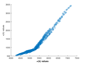
Figure 2: Coordinates of 750 scenarios of the aircraft allocation problem

The ranges of $\sigma(k)$ and $\kappa(k)$ are $[4260,7180]$ and $[530,3440]$, respectively. We adjust the number bins to evenly cover both ranges and create grids. Scenarios falling into the same grid will be treated as similar scenarios. When we set $\delta=29$, we have $100\times 100$ grids and we consolidate 415 scenarios. Using the remaining 335 scenarios, we obtain the same optimal solution as the published result. Furthermore, when we set $\delta=290$, we have only $10\times 10$ grids and we treat the scenarios, whose coordinates fall to the same grid, as similar scenarios. After clustering similar scenarios, we have 91 scenarios left. Using this reduced sample of 91 scenarios only, we still obtain the same optimal solution as the published result.

Example 4.

We now present the result of another well-known stochastic program, e.g., “LandS.” The problem description is in [11], and its second-stage decisions are integers. Our clustering method is applied to a sample of size $K=20,000$. Without clustering, the SAA will use an iid sample of size $K=20,000$, which implies that the mixed-integer program has 240,004 variables, and 240,000 variables among them are integers. It also indicates 140,002 mixed but mostly integer constraints. When we cluster half of the scenarios, the SAA with the reduced sample will have only 120,004 variables and 70,002 constraints. If we cluster scenarios with $\delta=0.05$, we cluster 18,159 scenarios, such that the equivalent mixed-integer program will have 22,096 variables and 12,889 constraints, i.e., a reduction of 89% scenarios, 90% variables and constraints.

The advantage of our method is significant. On an average computer, the computational time to solve SDP for the coordinate $(\kappa(k),\sigma(k))$ for each scenario polyhedron is less than 20 seconds for the LandS. For $K=20,000$ scenarios, it will take 240,000 seconds, i.e., less than 67 hours. Since clustering can be deployed to computer cluster, and all of the computational tasks could be deployed in parallel, the time would be greatly shortened. Supposing we have a computer cluster of 10 average computers, it will take less than 7 hours. The clustering time could be further shortened by coding the convex optimization solver, which currently uses Matlab, with more efficient languages. The reduced problem is significantly friendlier to solvers regarding the scale. Given the well-known difficulty of the integer program, such a reduction in the problem scale is always well justified.

6 Conclusion

In this paper, we propose an improvement to the SAA method and the key idea is to attach a measure of similarity, the coordinate $(\sigma(k),\kappa(k))$, to each sampled scenario $\xi^{k}$. We cluster the scenarios of similar measures to reduce the sample size. We show that the clustering method inherits both the consistency and convergence in probability of the SAA. The clustering method will significantly reduce a large enough sample to a small, but representative one to deliver a timely solution without compromising solution quality. The implementation of clustering would be a distributed computer cluster, in which the auxiliary computational tasks, e.g., calculating the Löwner-John Ellipsoid, and calculating the coordinate, would be completed by low-cost computers deployed in parallel rather than expensive supercomputers. The benefit of clustering is that it reduces the scale of the stochastic program to its fraction. In numerical examples, nearly 90% of the integer variables and constraints are clustered, i.e., removed. Also, the clustering method will highlight a subset of scenarios requiring more attention from decision-makers because these scenarios will generate a significant impact on the optimal solution, compared to the remaining scenarios.

This method is worth more intensive testing because not only it identifies a massive number of scenarios with uniquely valued coordinates, but also it preserves the nice theoretical results of SAA. This method would be established as an alternative way of sampling to solve the tractability issue of stochastic programming. Furthermore, this method may lead to a distributed computational infrastructure to solve stochastic programming. The practitioners can start the solving process long before when the solution is demanded. The coordinates of sampled scenarios would be separately calculated on low-cost computers, which are deployed as clusters. The solution quality will be continuously improved as more iid scenarios are processed.

ACKNOWLEDGMENT 
The authors gratefully acknowledge the continued support of the School of Business Administration, University of Dayton.

References

- Boyd and Vandenberghe [2004] Boyd, Stephen, Lieven Vandenberghe. 2004. Convex optimization. Cambridge University Press.
- Dantzig [2016] Dantzig, George. 2016. Linear programming and extensions. Princeton university press.
- Dupačová et al. [2003] Dupačová, Jitka, Nicole Gröwe-Kuska, Werner Römisch. 2003. Scenario reduction in stochastic programming. Mathematical Programming 95(3) 493–511.
- Dyer and Stougie [2006] Dyer, Martin, Leen Stougie. 2006. Computational complexity of stochastic programming problems. mathematical Programming 106(3) 423–432.
- Homem-de Mello [2008] Homem-de Mello, Tito. 2008. On rates of convergence for stochastic optimization problems under non–independent and identically distributed sampling. SIAM Journal on Optimization 19(2) 524–551.
- Homem-de Mello and Bayraksan [2014] Homem-de Mello, Tito, Güzin Bayraksan. 2014. Monte carlo sampling-based methods for stochastic optimization. Surveys in Operations Research and Management Science 19(1) 56–85.
- John [2014] John, Fritz. 2014. Extremum problems with inequalities as subsidiary conditions. Traces and emergence of nonlinear programming. Springer, 197–215.
- Kim et al. [2015] Kim, Sujin, Raghu Pasupathy, Shane G Henderson. 2015. A guide to sample average approximation. Handbook of simulation optimization. Springer, 207–243.
- Kleywegt et al. [2002] Kleywegt, Anton J, Alexander Shapiro, Tito Homem-de Mello. 2002. The sample average approximation method for stochastic discrete optimization. SIAM Journal on Optimization 12(2) 479–502.
- Leövey and Römisch [2015] Leövey, Hernan, Werner Römisch. 2015. Quasi-monte carlo methods for linear two-stage stochastic programming problems. Mathematical Programming 151(1) 315–345.
- Linderoth et al. [2006] Linderoth, Jeff, Alexander Shapiro, Stephen Wright. 2006. The empirical behavior of sampling methods for stochastic programming. Annals of Operations Research 142(1) 215–241.
- Rahimian et al. [2018] Rahimian, Hamed, Güzin Bayraksan, Tito Homem-de Mello. 2018. Identifying effective scenarios in distributionally robust stochastic programs with total variation distance. Mathematical Programming 1–38.
- Shapiro et al. [2009] Shapiro, Alexander, Darinka Dentcheva, Andrzej Ruszczyński. 2009. Lectures on stochastic programming: modeling and theory. SIAM.
- Sun and Freund [2004] Sun, Peng, Robert M Freund. 2004. Computation of minimum-volume covering ellipsoids. Operations Research 52(5) 690–706.
- Xiao and Zhang [2014] Xiao, Lin, Tong Zhang. 2014. A proximal stochastic gradient method with progressive variance reduction. SIAM Journal on Optimization 24(4) 2057–2075.