Fast Bayesian Restoration of Poisson Corrupted Images with INLA
Abstract
Photon-limited images are often seen in fields such as medical imaging. Although the number of collected photons on an image sensor statistically follows Poisson distribution, this type of noise is intractable, unlike Gaussian noise. In this study, we propose a Bayesian restoration method of Poisson corrupted image using Integrated Nested Laplace Approximation (INLA), which is a computational method to evaluate marginalized posterior distributions of latent Gaussian models (LGMs). When the original image can be regarded as ICAR (intrinsic conditional auto-regressive) model reasonably, our method performs very faster than well-known ones such as loopy belief propagation-based method and Markov chain Monte Carlo (MCMC) without decreasing the accuracy.
Keywords:
Probabilistic Image Processing, Image Restoration, Bayesian Modeling, Integrated Nested Laplace ApproximationI Introduction
Estimating the original image from a noisy observation is one of the representative issues in the field of image processing. So far, a lot of image denoising methods have been proposed, but many of them such as Wiener filter require the assumption of additive white Gaussian noise. However, for example, in medical X-ray imaging systems, the number of detected photons stochastically fluctuates following Poisson distribution[1].
From a Bayesian viewpoint, it is natural to adopt Poisson observation modeling explicitly, and then solve the inverse problem to deal with such images. In fact, some Bayesian methods to restore Poisson corrupted images have been already proposed. Le et al. introduced a variational model with total-variation regularization[2]. Lefkimmiatis et al. applied quadtree decomposition and then estimated parameters using expectation-maximization (EM) algorithm to handle Poisson noise[3]. Shouno derived the fixed point equations of loopy belief propagation (LBP) by approximating Poisson distribution with binomial distribution[4]. Furthermore, Tachella et al. compared the performances of multiple MCMC methods to restore Poisson corrupted images [5].
These methods are frequently used to evaluate the posterior (or its point estimate) of each pixel. In more general applications, Markov chain Monte Carlo (MCMC) methods succeeded due to their usability and accuracy. On the other hand, recently, integrated nested laplace approximation (INLA) is proposed by Rue et al. [6], then the validity has been reported mainly in the fields of spatial statistics and epidemiology [7]. For example, INLA is used disease mapping[8], analysing spatio-temporal evolutions of Ebola virus[9], and Bayesian outbreak detection[10]. Also there is a similar research to ours, INLA-based super-resolution method has been proposed [11].
INLA is a powerful framework to evaluate posterior marginals on latent Gaussian models (LGMs). LGM is a class of statistical models which includes a lot of standards, for example, auto-regressive (AR), conditional auto-regressive (CAR), and generalized linear mixture (GLM) models[7, 12]. INLA consists of two layers of units: latent variables following Gaussian Markov random field (GMRF) and their observations. Latent variables requires normality on their interactions, but observation processes do not. INLA is based on Laplace approximations and numerical integrations as the name suggests. As the interface for using INLA, R-INLA is provided by R-INLA project 111http://www.r-inla.org/.
In this study, we try applying INLA to image restoring as the application to the new field, through dealing with Poisson corrupted images. When the original image seems to be reasonable to assume intrinsic CAR (ICAR) model, which means almost of adjacent pixels do not vary sharply, the proposed method obtained equal to the result by an MCMC simulation rapidly.
This paper organized as following: first, we give a brief description of INLA in Section 2. Then, we explain our model to infer the original images in Section 3, and to evaluate proposed method we show configurations and results of the computational simulations in Section 4. At last, in Section 5, we summarize and conclude about our method.
II Methodology
II-A Latent Gaussian Models
A latent Gaussian Models (LGM) is a class of statistical models, which include many commonly used statistical models such as auto-regressive (AR) model, conditional auto-regressive (CAR) model, and generalized linear mixture (GLM) model.
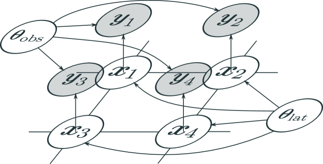
Fig.1 shows the outline of an LGM. In LGMs, latent variables follow Gaussian Markov random field (GMRF)
| (1) |
where is a set of hyperparameters of latent GMRF. In addition, mean vector and precision matrix are parameterized by .
Observations should be conditionally independent and identically distributed on a parameter set
| (2) |
and conditional distribution must be belong to exponential family. Hereafter, for simplicity, we will put hyperparameter sets into ,
| (3) |
II-B Integrated Nested Laplace Approximation
Integrated Nested Laplace Approximation (INLA) is a fast and accurate method to approximate posterior distributions of LGMs[6]. Especially when the number of hyperparamters is small (empirically [7]), INLA performs very faster than Markov chain Monte Carlo (MCMC).
In LGMs, our aim is to get marginalized posteriors of hyperparameters
| (4) |
and latent variables
| (5) |
In equation (4), each term in the numerator can be calculated by forward computation, but the denominator can not. Hence, first we apply Laplace (or simplified Laplace, which can fit with a skew normal distribution[13, 6]) approximation to the denominator
| (6) |
where denotes an approximation of .
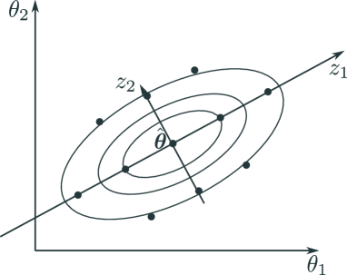
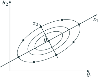
For latent variables (5), applying numerical integration as following:
-
1.
Exploring the mode of using an optimization algorithm (e.g., quasi-Newton method) with respect to .
- 2.
-
3.
Calculating at arranged points, where is the index of each point.
- 4.
III Our Model
III-A ICAR Models
To use INLA, we should choose a latent structure carefully. This is because the computaional performance of INLA strongly depends on the number of hyperparameters of the LGM.
ICAR model is one of the commonly used representations of spatial interaction[15]. In ICAR model, has interaction with , where indicates the set of indices of nearest neighbor nodes of (for simplicity, each variable is assumed to be a scalar value). Here it assumed that follows
| (8) |
where is the hyperparameter indicates variance between nodes. This model means some assumptions on :
-
•
Each node hardly differs from adjacent ones.
-
•
The similarity between adjacent nodes is controlled by the fixed effect .
-
•
As is increasing, the variance of decreases.
At a glance, this model seems not to be inappropriate. However, the precision matrix of does not satisfy the condition of positive definiteness, then ICAR models become improper. Therefore, we need to regularize them to guarantee its computational stabiliy.
III-B Proper ICAR Models
To guarantee properness of ICAR models, two reguralization ways are frequently implemented: scaling by or adding extra terms to the parameters of equation (8). We adopt the latter strategy, since the number of detected photons must be non-negative. We use following proper ICAR model for the latent GMRF of adopted model,
| (9) |
where is the extra hyperparameter for stability. In this study, we configure interaction in a grid without periodic boundary condition for the latent GMRF to deal with images. For instance, we consider the probability of a non-corner pixel of an image. Here, we can deform equation (9) into
| (10) |
where
| (11) |
III-C Observation Model
In photon-limited images, the number of observated photons fluctuates as following Poisson distribution with the true value . Hence, we use
| (12) |
as the observation model straightforwardly, and is assumed to be independent from other observations with given . Therefore, the joint distribution of becomes
| (13) |
III-D Hyperpriors
In our model described above, we have two hyperparameters and . As their hyperpriors, we use uninformative prior on .
IV Experiments
IV-A Preprocessing
To handle general images with our model and control their contrast, we firstly transform the pixel value in the original image into positive value , where the original image and its transformation consist of pixels. In particular, we give linear transformation
| (14) |
where and are given parameters indicate maximum and minimum values of respectively, then and are the maximum and minimum values of . We can control the range of intensity by varying and .
IV-B Evaluation Criteria
In our simulations, we use peak signal-to-noise ratio (PSNR) and structural similarity (SSIM)[16] to measure similarities between original and denoised images. PSNR is defined by
| (15) | |||
| (16) |
where and denote images have pixels. Here, PSNR just focuses on the each corresponding pixel value. To consider the perceptual similarity between two images, we also introduce SSIM for the evaluation criterion. SSIM is defined as follows:
| (17) |
where and are the means of and respectively, and and are the variances of and respectively. Also, indicates the covariance between and . In addition, are small positive real numbers for the stability.
Here, PSNR can take from to infinity, and SSIM is in range of to . In each criterion, the larger value is, the closer two images are.
IV-C Simulations


original
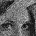
corrupted
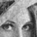
INLA

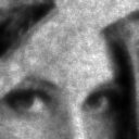
MCMC
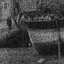
LBP
original
corrupted
INLA

MCMC
LBP
original
corrupted
INLA
MCMC
LBP

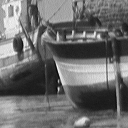
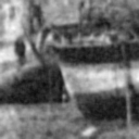
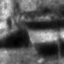
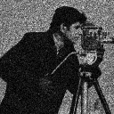
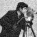
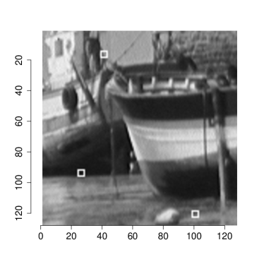
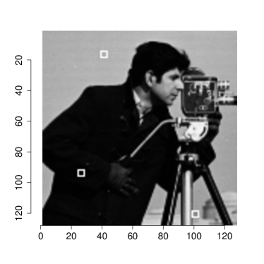
In this study, we compared denoising simulation results with INLA, MCMC (Hamiltonian Monte Carlo with No U-Turn Sampler[17, 18]), and LBP using the described model in Section 3. We simulated MCMC for 2000 steps and set first 1000 steps as burn-in. As the original images, we use “Lena”, “Boat”, and “Cameraman” for the evaluation (in Fig.3). Here, we fixed the contrast parameters as and , and ran the simulations on the computer has AMD Ryzen Threadripper 2990WX (32 cores, 3.0 GHz) as its CPU and 128 GB memory. To compute point estimates of , we used expected a posteriori (EAP) estimation in INLA and MCMC.
| Image | Method | PSNR | SSIM | Time(s) |
|---|---|---|---|---|
| Lena | INLA | 22.24 | 0.966 | 226.8 |
| MCMC | 24.97 | 0.968 | 2083.5 | |
| LBP | 21.77 | 0.928 | 18794.7 | |
| Boat | INLA | 21.76 | 0.947 | 209.5 |
| MCMC | 24.03 | 0.960 | 1585.3 | |
| LBP | 21.50 | 0.915 | 18891.5 | |
| Cameraman | INLA | 10.88 | 0.916 | 113.5 |
| MCMC | 21.82 | 0.956 | 1360.7 | |
| LBP | 19.61 | 0.923 | 18809.8 |
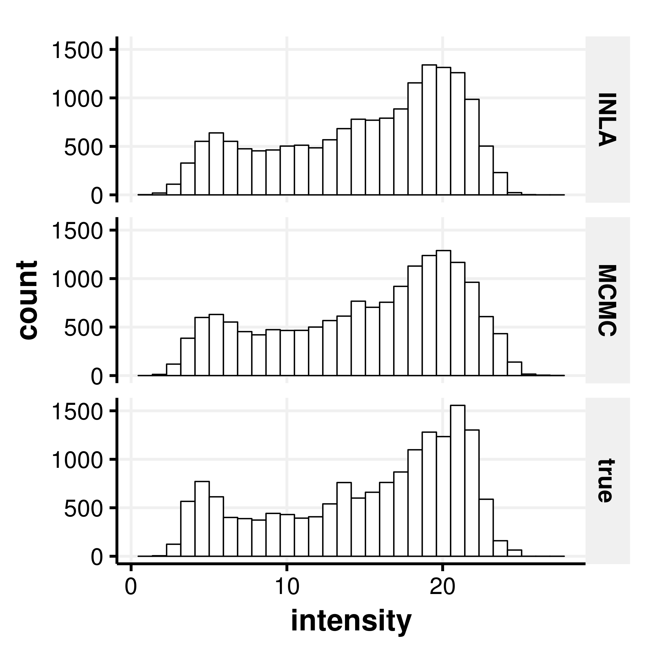
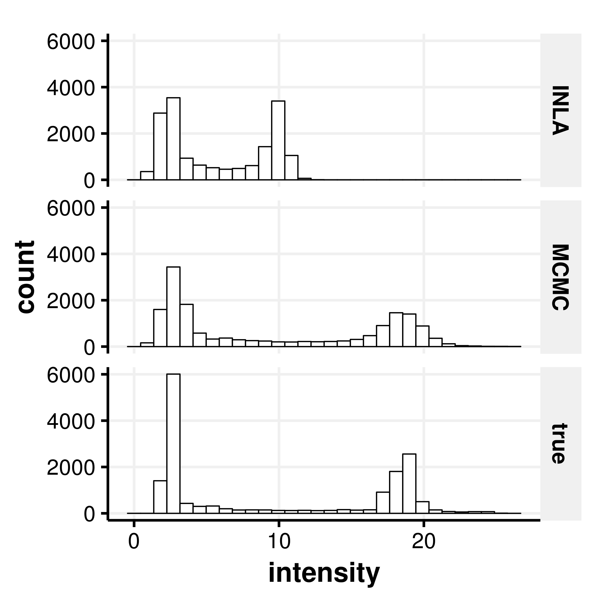
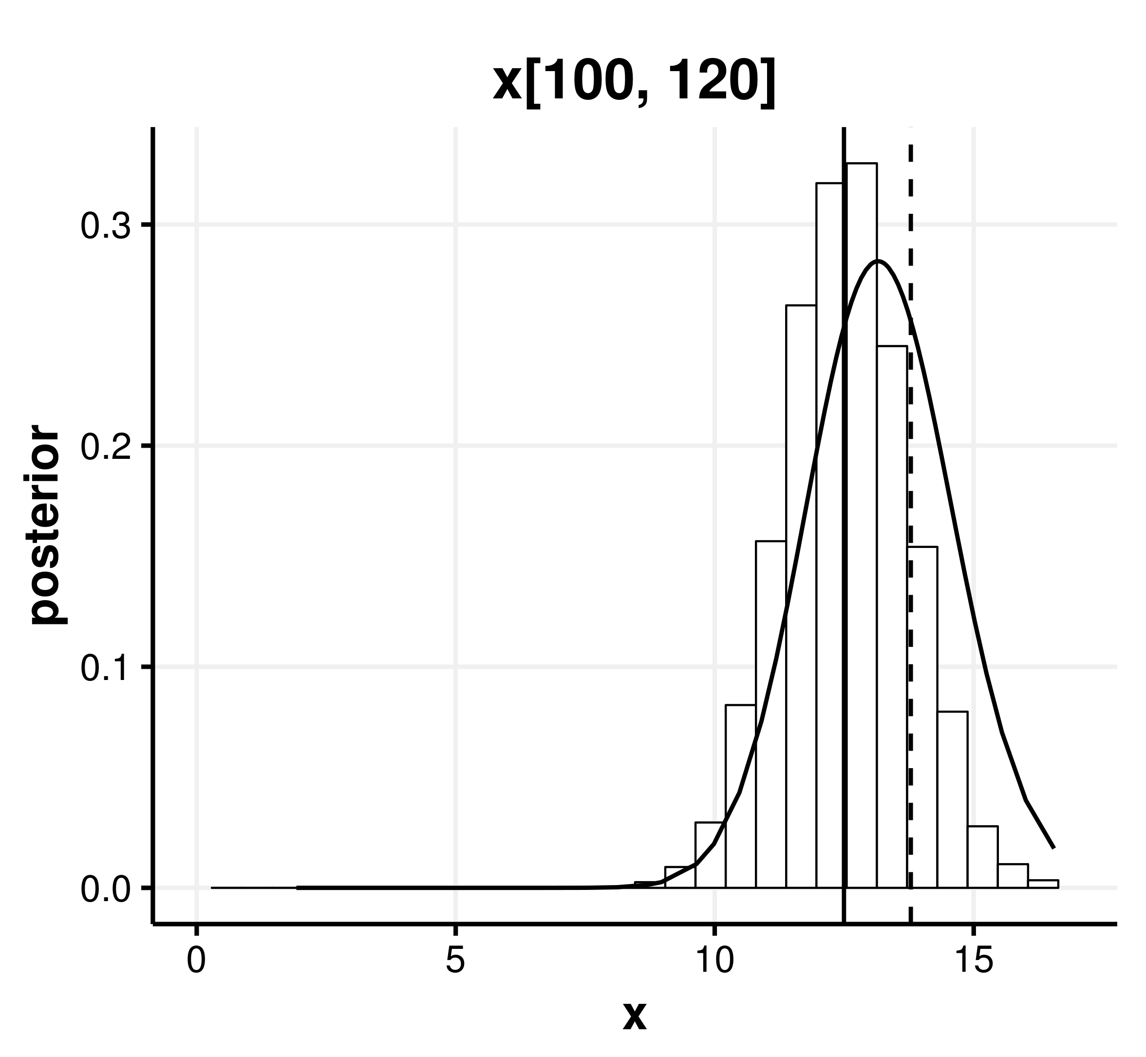
Table I shows the comparison of results of INLA, MCMC, and LBP. In Table I, we can find that INLA is very faster than other algorithms with little decreasing PSNR and SSIM from MCMC, expect for “Cameraman”. LBP is too slow because it requires spectral decomposition of an matrix in its algorithm. Fig.4 is the denoised images. Qualitatively, the images restored by INLA look clearer and unhazier than by other methods on a whole. On the other hand, we could not estimate the original “Cameraman” appropriately using INLA (Fig.4(c)). Specifically, the result of INLA is apparently different from others in its brightness. Then, to give additional consideration, we present histograms of intensities in Fig.5. Seeing Fig.5(b), we can find that brighter pixels have been hardly restored in “Cameraman”. In “Lena”, the shape of true histogram is slightly flat. In contrast, the true histogram of “Cameraman” has two sharp peaks. Therefore, it is conceivable that the error of INLA mainly caused by this illness. In this case, INLA might fail to estimate the hyperparameters due to the illness of the original image, then also failed to get appropriate posteriors with respect to the latent variables.
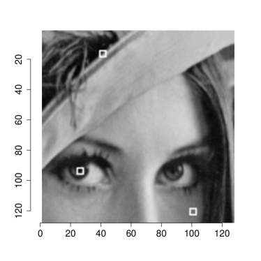
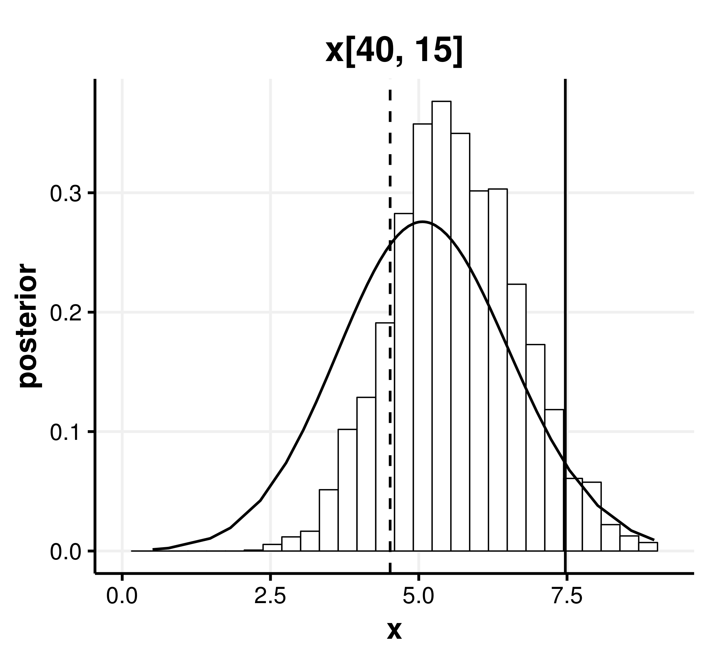
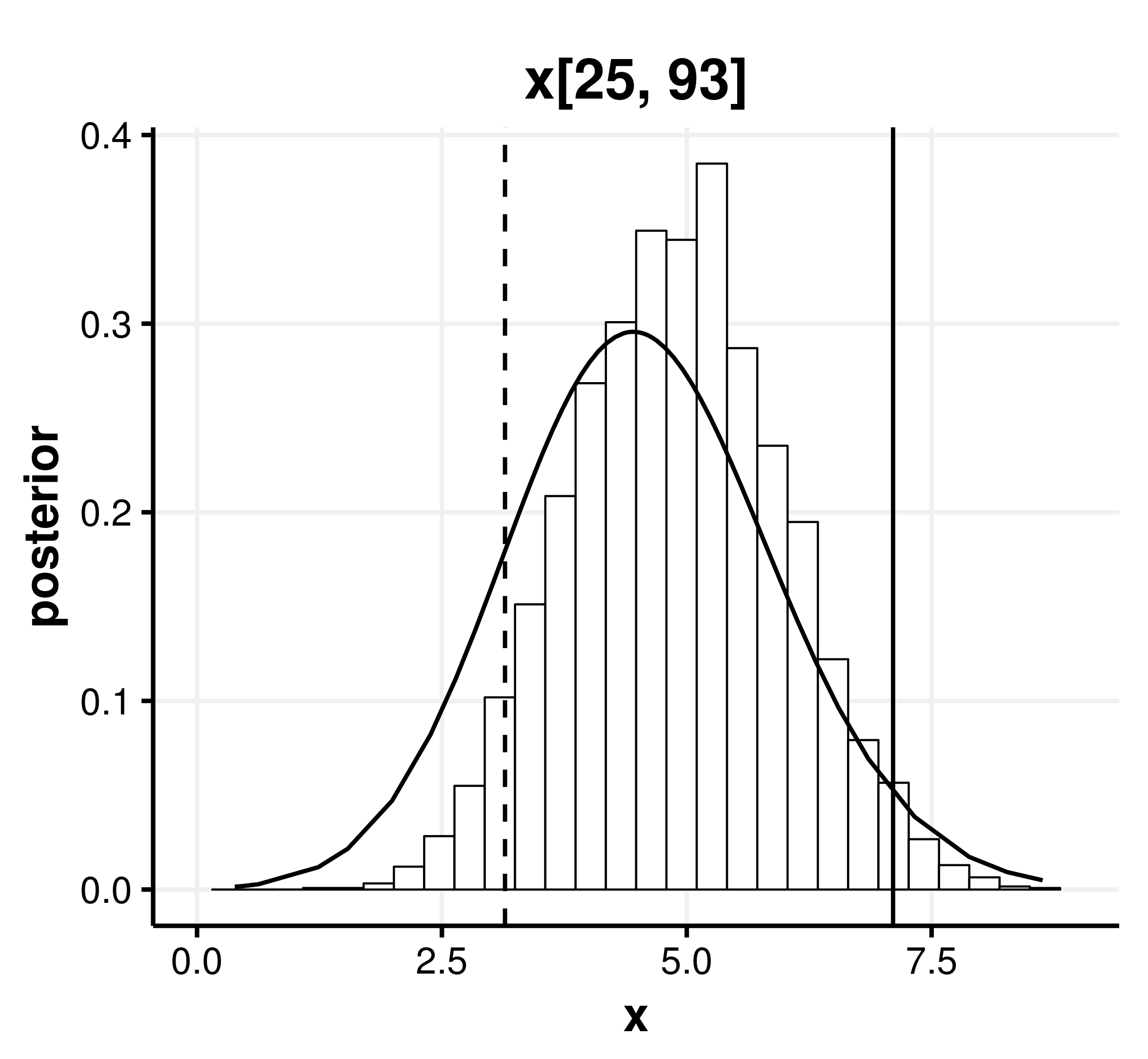
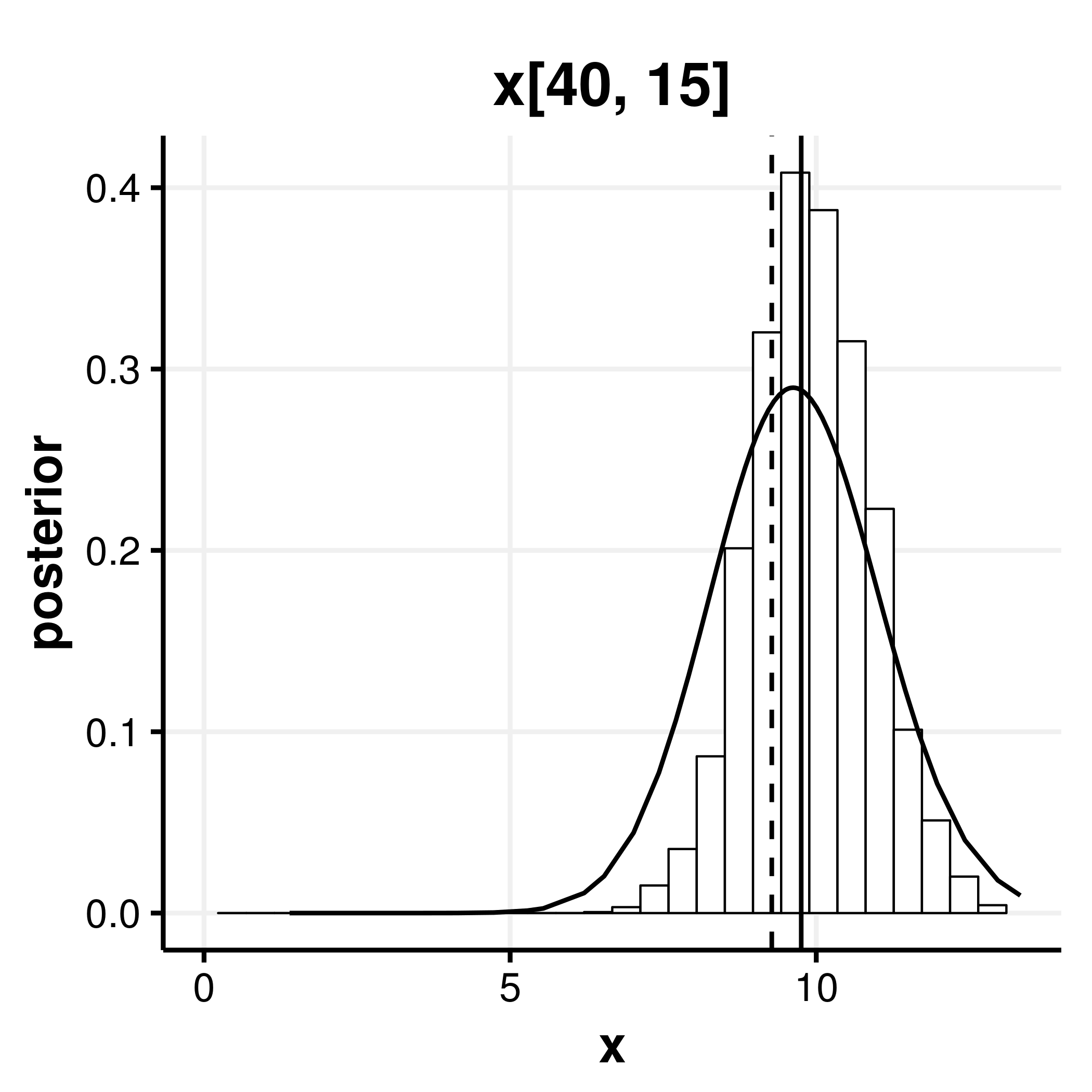
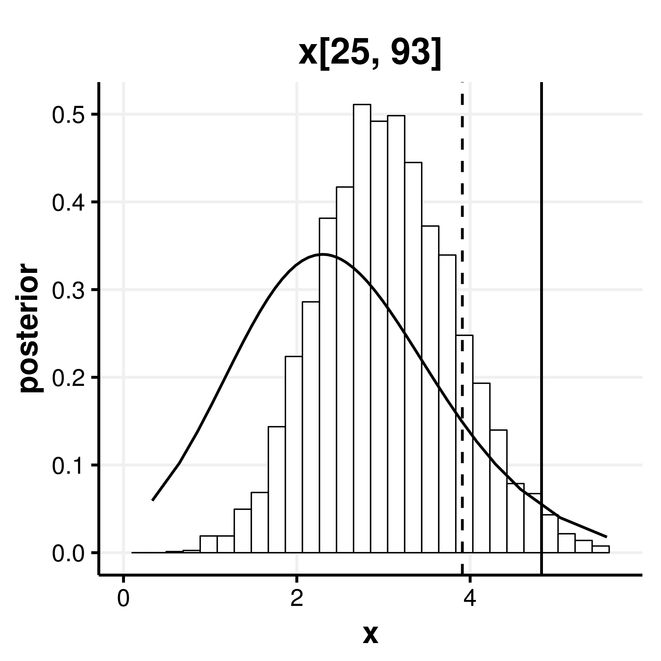
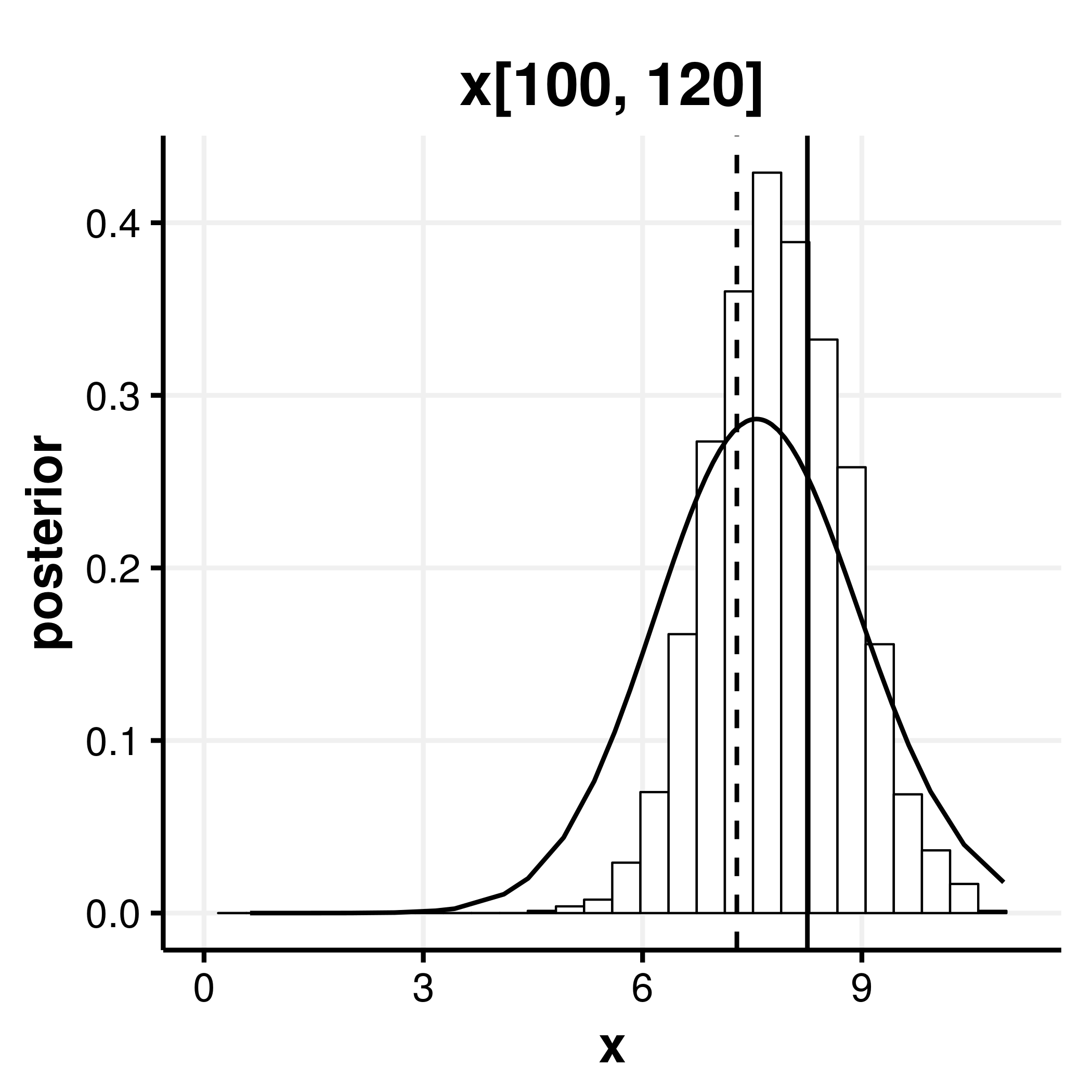
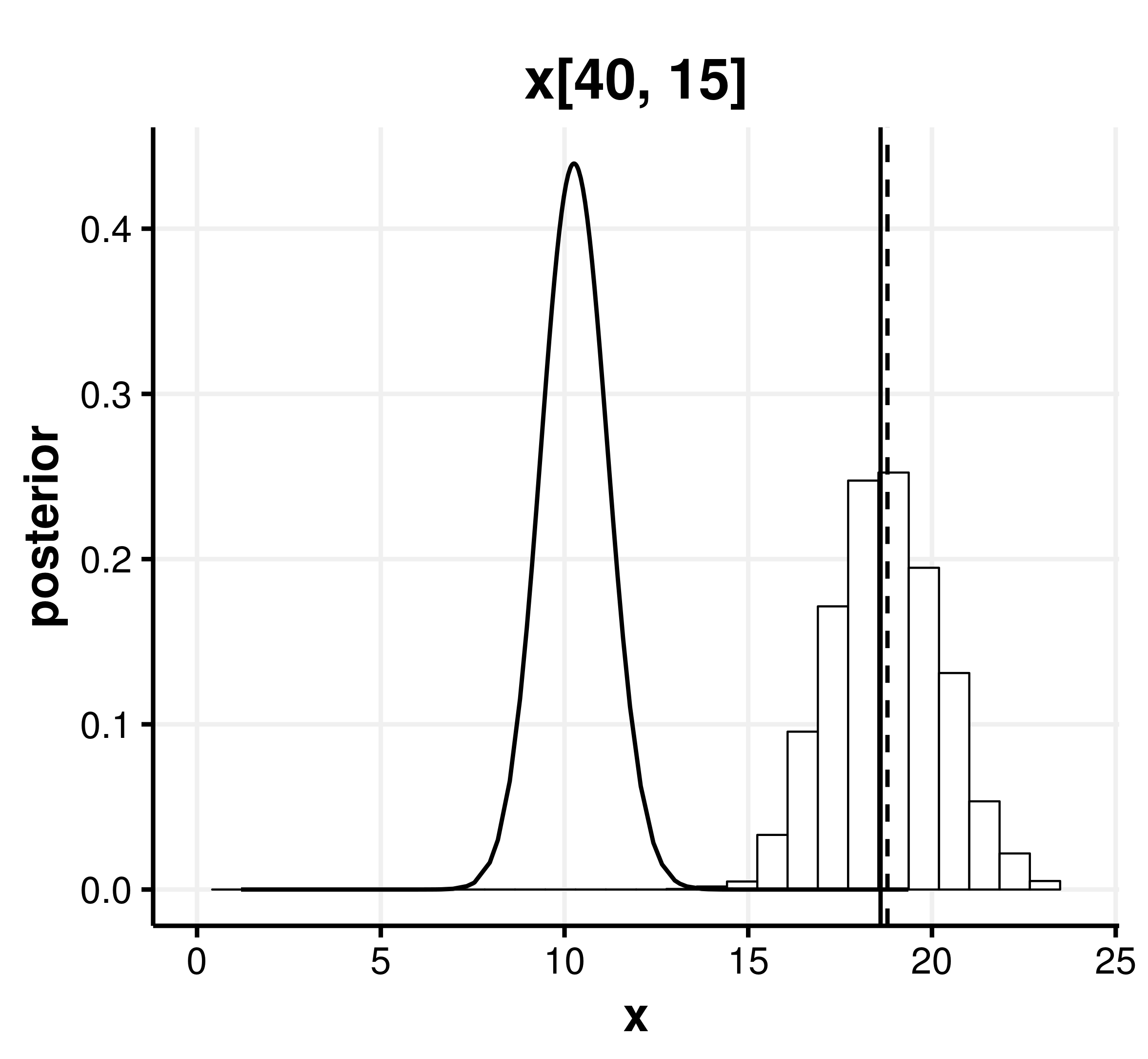
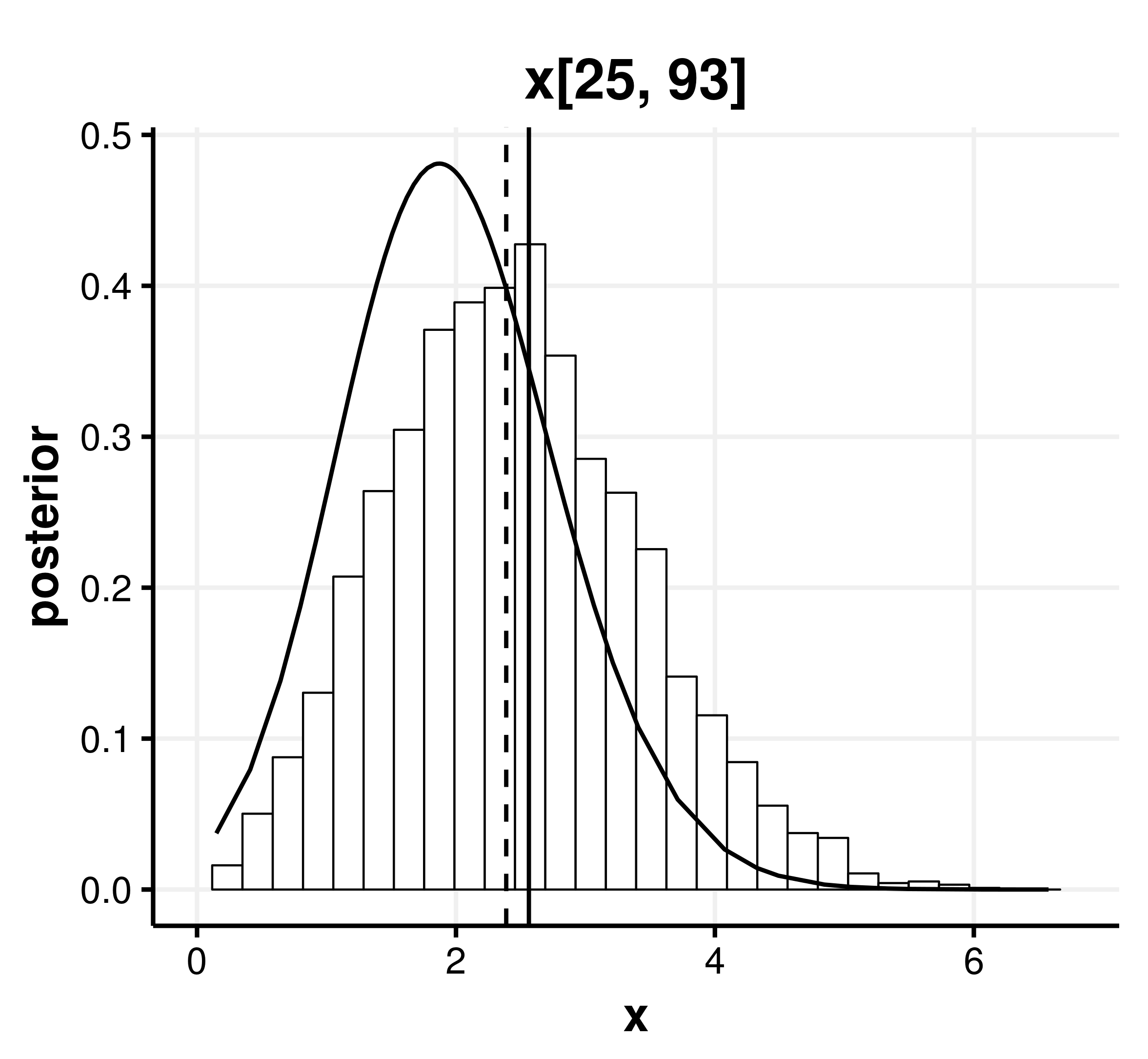
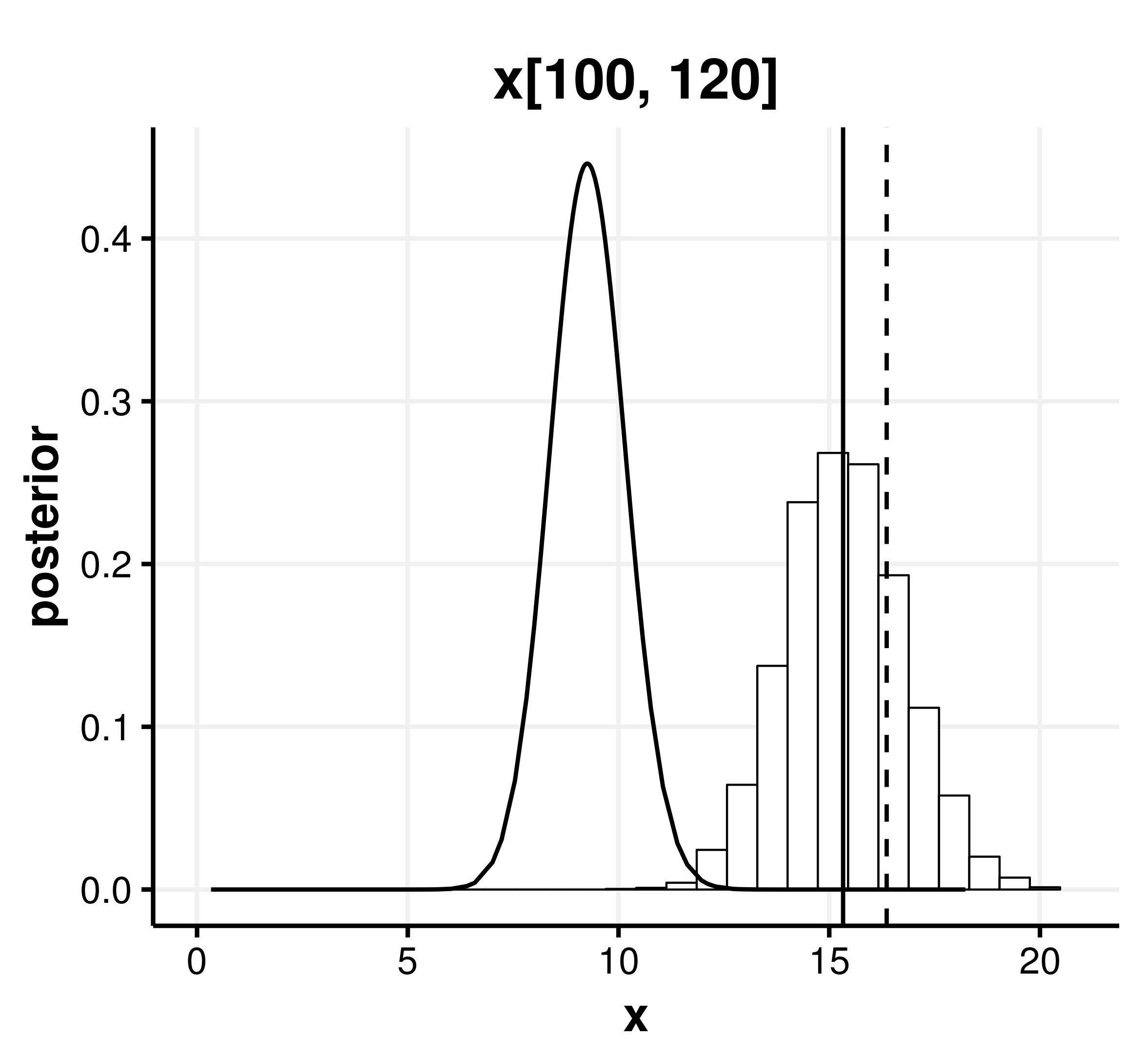
Additionaly we indicate evaluated posteriors or its point estimates of some pixels of each image in Fig.6. The differences of posteriors between INLA and MCMC are unnoticeable in “Lena” (Fig.6(a)). In “Boat”, the pixel which is near a sharp edge is slightly different the histogram by MCMC. Moreover, we can also find that brighter pixels could not be restored in “Cameraman” by seeing Fig.6(c).
V Conclusion
In this study, we proposed and evaluated a denoising methods for Poisson corrupted images based on INLA. INLA requires an assumption of GMRF to latent variables. Hence, its accuracy decreases when the assumption is inappropriate. Whereas when the assumption is suitable for the original image, we can reduce much time compared to other Bayesian computational algorithms, such as LBP or MCMC with enough accuracy.
As a future work, we can also consider to use other models for latent models. For example, to apply segmentation to noisy image firstly, and then evaluate posteriors of each segmentation independently. In addition, we should adopt our method to real X-ray imaging data, and then evaluate its effectivity.
References
- [1] A. K. Boyat and B. K. Joshi, “A review paper: Noise models in digital image processing,” arXiv:1505.03489 [cs], May 2015, arXiv: 1505.03489. [Online]. Available: http://arxiv.org/abs/1505.03489
- [2] T. Le, R. Chartrand, and T. J. Asaki, “A variational approach to reconstructing images corrupted by poisson noise,” Journal of mathematical imaging and vision, vol. 27, no. 3, pp. 257–263, 2007.
- [3] S. Lefkimmiatis, M. Petros, and P. George, “Bayesian inference on multiscale models for poisson intensity estimation: Applications to photon-limited image denoising,” IEEE Transactions on Image Processing, vol. 18, no. 8, pp. 1724–1741, Aug 2009.
- [4] H. Shouno, “Bayesian image restoration for Poisson corrupted image using a latent variational method with Gaussian MRF,” IPSJ Online Transactions, vol. 8, no. 0, pp. 15–24, 2015. [Online]. Available: https://www.jstage.jst.go.jp/article/ipsjtrans/8/0/8_15/_article
- [5] J. Tachella, Y. Altmann, M. Pereyra, S. McLaughlin, and J. Y. Tourneret, “Bayesian restoration of high-dimensional photon-starved images,” in 2018 26th European Signal Processing Conference (EUSIPCO). Rome: IEEE, Sep. 2018, pp. 747–751. [Online]. Available: https://ieeexplore.ieee.org/document/8553175/
- [6] H. Rue, S. Martino, and N. Chopin, “Approximate Bayesian inference for latent Gaussian models by using integrated nested Laplace approximations,” Journal of the Royal Statistical Society: Series B (Statistical Methodology), vol. 71, no. 2, pp. 319–392, Apr. 2009. [Online]. Available: https://rss.onlinelibrary.wiley.com/doi/abs/10.1111/j.1467-9868.2008.00700.x
- [7] H. Rue, A. Riebler, S. H. Sørbye, J. B. Illian, D. P. Simpson, and F. K. Lindgren, “Bayesian computing with INLA: A review,” Annual Review of Statistics and Its Application, vol. 4, no. 1, pp. 395–421, 2017. [Online]. Available: https://doi.org/10.1146/annurev-statistics-060116-054045
- [8] B. Schrödle and L. Held, “Spatio-temporal disease mapping using inla,” Environmetrics, vol. 22, no. 6, pp. 725–734, 2011. [Online]. Available: https://onlinelibrary.wiley.com/doi/abs/10.1002/env.1065
- [9] E. Santermans, E. Robesyn, T. Ganyani, B. Sudre, C. Faes, C. Quinten, W. Van Bortel, T. Haber, T. Kovac, F. Van Reeth, M. Testa, N. Hens, and D. Plachouras, “Spatiotemporal evolution of Ebola virus disease at sub-national level during the 2014 West Africa epidemic: Model scrutiny and data meagreness,” PLOS ONE, vol. 11, no. 1, 2016. [Online]. Available: https://doi.org/10.1371/journal.pone.0147172
- [10] M. Salmon, D. Schumacher, K. Stark, and M. Höhle, “Bayesian outbreak detection in the presence of reporting delays,” Biometrical Journal, vol. 57, no. 6, pp. 1051–1067, 2015. [Online]. Available: https://onlinelibrary.wiley.com/doi/abs/10.1002/bimj.201400159
- [11] M. O. Camponez, E. O. T. Salles, and M. Sarcinelli-Filho, “Super-resolution image reconstruction using nonparametric bayesian inla approximation,” IEEE Transactions on Image Processing, vol. 21, no. 8, pp. 3491–3501, Aug. 2012.
- [12] T. Opitz, “Latent Gaussian modeling and INLA: A review with focus on space-time applications,” Journal of the French Statistical Society, vol. 158, no. 3, pp. 62–85, 2017.
- [13] A. Azzalini and A. Capitanio, “Statistical applications of the multivariate skew normal distribution,” Journal of the Royal Statistical Society: Series B (Statistical Methodology), vol. 61, no. 3, pp. 579–602, 1999. [Online]. Available: https://rss.onlinelibrary.wiley.com/doi/abs/10.1111/1467-9868.00194
- [14] G. E. P. Box and K. B. Wilson, “On the experimental attainment of optimum conditions,” Journal of the Royal Statistical Society. Series B (Methodological), vol. 13, no. 1, pp. 1–45, 1951. [Online]. Available: http://www.jstor.org/stable/2983966
- [15] J. Besag and C. Kooperberg, “On conditional and intrinsic autoregression,” Biometrika, vol. 82, no. 4, pp. 733–746, 1995. [Online]. Available: https://www.jstor.org/stable/2337341
- [16] Z. Wang, A. C. Bovik, H. R. Sheikh, and E. P. Simoncelli, “Image quality assessment: from error visibility to structural similarity,” IEEE transactions on image processing, vol. 13, no. 4, pp. 600–612, 2004.
- [17] S. Duane, A. D. Kennedy, B. J. Pendleton, and D. Roweth, “Hybrid Monte Carlo,” Physics Letters B, vol. 195, no. 2, pp. 216 – 222, 1987. [Online]. Available: http://www.sciencedirect.com/science/article/pii/037026938791197X
- [18] M. D. Hoffman and A. Gelman, “The no-u-turn sampler: adaptively setting path lengths in hamiltonian monte carlo.” Journal of Machine Learning Research, vol. 15, no. 1, pp. 1593–1623, 2014.