Point in, Box out: Beyond Counting Persons in Crowds

Abstract

Modern crowd counting methods usually employ deep neural networks (DNN) to estimate crowd counts via density regression. Despite their significant improvements, the regression-based methods are incapable of providing the detection of individuals in crowds. The detection-based methods, on the other hand, have not been largely explored in recent trends of crowd counting due to the needs for expensive bounding box annotations. In this work, we instead propose a new deep detection network with only point supervision required. It can simultaneously detect the size and location of human heads and count them in crowds. We first mine useful person size information from point-level annotations and initialize the pseudo ground truth bounding boxes. An online updating scheme is introduced to refine the pseudo ground truth during training; while a locally-constrained regression loss is designed to provide additional constraints on the size of the predicted boxes in a local neighborhood. In the end, we propose a curriculum learning strategy to train the network from images of relatively accurate and easy pseudo ground truth first. Extensive experiments are conducted in both detection and counting tasks on several standard benchmarks, e.g. ShanghaiTech, UCF_CC_50, WiderFace, and TRANCOS datasets, and the results show the superiority of our method over the state-of-the-art.

1 Introduction

Counting people in crowded scenes is a crucial component for a wide range of applications including video surveillance, safety monitoring, and behavior modeling. It is a highly challenging task in dense crowds due to heavy occlusions, perspective distortions, scale variations and varying density of people. Modern regression-based methods [27, 49, 41, 25, 22, 20, 39] cast the problem as regressing a density distribution map whose integral over the map gives the people count within that image (see Fig 1: Left). Owing to the advent of deep neural networks (DNN) [17], remarkable progress has been achieved in these methods. They do not require annotating the bounding boxes but only the points of person heads at training. Yet, as a consequence, they can not provide the detection of persons at testing, neither.

The detection-based methods, which cast the problem as detecting each individual in the crowds (see Fig 1: Right), on the other hand, have not been largely explored in recent trends due to the lack of bounding box annotations. Liu et al. [22] have tried to manually annotate on partial of the bounding boxes in ShanghaiTech PartB (SHB) dataset [49] and train a fully-supervised Faster R-CNN [32]. They combine the detection result with regression result for crowd counting. Notwithstanding their efforts and obtained improvements, they did not report results on datasets like SHA [49] and UCF_CC_50 [13], which have crowds on average five and ten times denser than that of SHB.

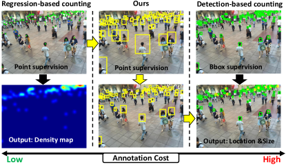
Figure 1: Comparison of our PSDDN with representative regression- and detection-based crowd counting methods regarding their annotation costs for input and their output information.

Annotating the bounding boxes of persons for training images can be a great challenge in crowd counting datasets. Meanwhile, knowing the person size and locations in a crowd at test stage is also very important; for example, in video surveilance, it enables person recognition [37], tracking [33], and re-identification [21]. Recently, some researchers [18, 14] start to work on this issue with point supervision by employing segmentation frameworks [18] or regressing the localization maps [14] to simultaneously localize the persons and predict the crowd counts. Because they only use point-level annotations, they simply focus on localizing persons in the crowds, but do not consider predicting the proper size.

To be able to predict the proper size and locations of persons and meanwhile bypass the need for expensive bounding box annotations, we introduce a new deep detection network using only point-level annotations on person heads (see Fig. 1: Middle). Although the real head size is not annotated, the intuition of our work is based on the observations that i) when two persons are close enough, their head distance indeed reflects their head size (similar to [49]); ii) due to the perspective distortion, person heads in the same horizontal line usually have similar size and gradually become smaller in the remote (top) area of the image. Both observations are common in crowd counting scenarios. They inspire us to mine useful person size information from head distances, and generalize a reliable point-supervised person detector with the help of head point annotations and size correlations in local areas.

To summarize, our work tries to tackle a very challenging yet meaningful task which is never handled by before; we propose a point-supervised deep detection network (PSDDN) for crowd counting which takes in cheap point-level annotations on person heads at training stage and produces out elaborate bounding box information on person heads at test stage. The contribution is three-fold:

• We propose a novel online pseudo ground truth updating scheme which initializes the pseudo ground truth bounding boxes from point-level annotations (Fig. 1: Middle top) and iteratively updates them during training (Fig. 1: Middle bottom). The initialization is based on the nearest neighbor head distances.

• We introduce a novel locally-constrained regression loss in the point-supervised setting which encourages the predicted boxes in a local band area to have the similar size. The loss function is inspired from the perspective distortion impact on the person size in an image [39, 6, 47];

• We propose a curriculum learning strategy [3] to feed the network with training images of relatively accurate and easy pseudo ground truth first. The image difficulty is defined over the distribution of the nearest neighbor head distances within each image.

In extensive experiments, we show that (1) PSDDN performs close to those regression-based methods in crowd counting task on ShanghaiTech and UCF_CC_50 datasets; outperforms the state-of-the-arts by integrating with them. (2) In the mean time it produces very competitive results in person detection task on ShanghaiTech, UCF_CC_50, and WiderFace [46] datasets. (3) We also evaluate PSDDN on the vehicle counting dataset TRANCOS [10] to show its generalizability in other detection and counting tasks.

2 Related works

We present a survey of related works in three aspects: (1) detection-based crowd counting; (2) regression-based crowd counting; and (3) point-supervision.

2.1 Detection-based crowd counting

Traditional detection-based methods often employ motion and appearance cues in video surveillance to detect each individual in a crowd [43, 5, 29]. They are suffered from heavy occlusions among people. Recent methods in the deep fashion learn person detectors relying on exhaustive bounding box annotations in the training images [42, 22]. For instance, [22] have manually annotated the bounding boxes on partial of SHB and trained a Faster R-CNN [32] for crowd counting. The annotation cost can be very expensive and sometimes impractical in very dense crowds. Our work instead uses only the point-level annotations to learn the detection model.

There are some other works particularly focusing on small object detection, e.g. faces [12, 26, 1]. [12] proposed a face detection method based on the proposal network [32] while [26] proposed to detect and localize faces in a single stage detector like SSD [23]. The face crowds tackled in these works are however way less denser than those in crowd counting works; moreover, these works are typically trained with bounding box annotations.

2.2 Regression-based crowd counting

Earlier regression-based methods regress a scalar value (people count) of a crowd [6, 7, 13]. Recent methods instead regress a density map of a crowd; crowd count is obtained by integrating over the density map. Due to the use of strong DNN features, remarkable progress has been achieved in recent methods [49, 35, 41, 25, 22, 24, 31, 14, 39]. More specifically, [41] designed a contextual pyramid DNN system. It consists of both a local and global context estimator to perform patch-based density estimation. [24] leveraged additional unlabeled data from Google Images to learn a multi-task framework combining both counting information in the labeled data and ranking information in the unlabeled data.  [31] proposed an iterative crowd counting network which first produces the low-resolution density map and then uses it to further generate the high-resolution density map. Despite the significant improvements achieved in these regression-based methods, they are usually not capable of predicting the exact person location and size in the crowds.

[22, 18, 14] are three most similar works to ours. [22] designed a so-called DecideNet to estimate the crowd density by generating detection- and regression-based density maps separately; the final crowd count is obtained with the guidance of an attention module. [14] introduced a new composition loss to regress both the density and localization maps together, such that each head center can be directly inferred from the localization map. [18] employed the hourglass segmentation network [34] to segment the object blobs in each image for crowd counting; instead of using per-pixel segmentation labels, they use only point-level annotations [2]. Our work is similar to [22] in the sense we both train a detection network for crowd counting; while [22] trained a fully-supervised detector using bounding box annotations, we train a weakly-supervised detector using only point-level annotations. Our work is also similar to [14, 18] where we all use point-level annotations; unlike our method, [14, 18] simply focus on person localization whereas we aim to predict both the localization and proper size of the person. Apart from all above, we also notice that we firstly evaluate the detection results on the dense crowd counting datasets i.e. ShanghaiTech and UCF_CC_50.

2.3 Point supervision

Point supervision scheme has been widely used in human pose estimation to annotate key-points of human body parts [16, 30, 36]; while in object detection or segmentation, it has often been employed to reduce the annotation time [4, 44, 45, 2, 28]. For example, Bearman et al. [2] conducted semantic segmentation by asking the annotators to click anywhere on a target object while Papadopoulos et al. [28] asked the annotators to click on the four physical points on the object for efficient object annotations. The points can be collected either once offline [2] or in an online interactive manner [4, 44, 45]. We collect the points once and only use them at training time.

3 Method

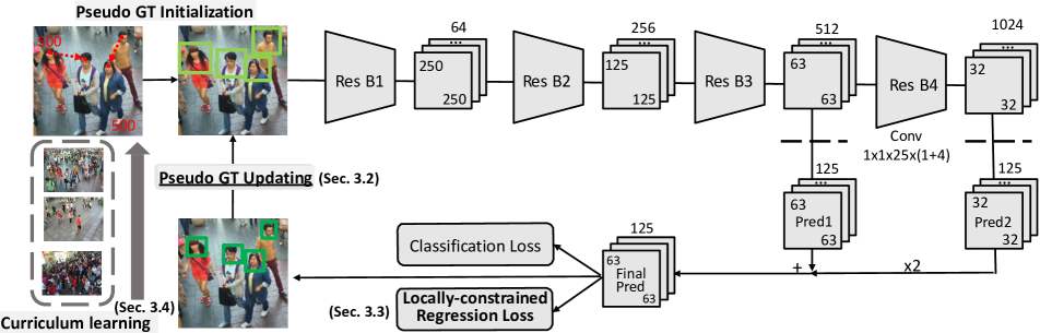
Figure 2: Network overview of PSDDN using only point-level annotations. Res B1 - B4 denotes the ResNet block adopted from ResNet-101 [11]. Person detection is conducted on two scales after Res B3 and B4; their predictions (Pred1 and Pred2) are summed up to produce the final prediction (Final Pred). We propose an online pseudo ground truth updating scheme which includes pseudo ground truth initialization and updating; a novel locally-constrained regression loss which encourages the predicted boxes in a local area to have the similar size. A curriculum learning strategy is proposed to train the network from images of relatively accurate pseudo ground truth first.

3.1 Overview

Our model is based on the widely used anchor based detection framework, such as RPN [32] and SSD [23]. The network architecture is shown in Fig. 2 where we adopt our backbone from ResNet-101 with four ResNet blocks (Res B1- B4) [11]. Likewise in [12], the outputs from Res B3 and Res B4 are taken to connect with two detection layers with different scales of anchors, respectively. The detection layer is a 1 x 1 convolutional layer that has the output of $N\times N\times T\times(1+4)$, where $N$ is the output length of feature maps and $T$ is the anchor set size (25 in our work). The aspect ratios of the predefined anchors are adapted from [32] by referring to the centroid clustering of the nearest neighbor distance between person heads. For each anchor, we predict 4 offsets relative to its coordinates and 1 score for classification. Prediction Pred2 is up-sampled to the same resolution with Pred1 and added together to produce the final map Final Pred. The multi-task loss of bounding box classification and regression is applied in the end.

We extend the framework to point-supervised crowd counting with modules marked in bold in Fig .2: a novel online ground truth (GT) updating scheme is firstly presented which incorporates initializing pseudo GT bounding boxes from point-level annotations and updating them during training. Afterwards, a locally-constrained regression loss is specifically proposed for bounding box regression with point-supervision. In the end, we introduce a curriculum learning strategy to train our model from images of relatively accurate pseudo ground truth first.

3.2 Online ground truth updating scheme

Pseudo ground truth initialization. To train a detection network, we need to first initialize the ground truth bounding boxes from head point annotations. We follow the inspiration in [49] that the head size is indeed related to the distance between the centers of two neighboring heads in crowded scenes. We use it to estimate the size of a bounding-box $g$ as the center distance $d(g,{\mathrm{NN}_{g}})$ from this head $g$ to its nearest neighbor ${\mathrm{NN}_{g}}$ (see Fig. 2: red dotted line). This makes a square bounding box; we find the corresponding anchor box that has the closest size to this square box as our initialization. We call the initialized bounding boxes pseudo ground truth. Some examples are shown in Fig. 1: Middle top. The estimations in dense crowds (top) are close to the real ground truth while in sparse crowds (bottom) are often bigger.

Pseudo ground truth updating. To train the detection network, we select positive and negative samples from the pre-defined anchors through their IoU (intersection-over-union) with the initialized pseudo ground truth. A binary classifier is trained over the selected positives and negatives so as to score each anchor proposal. Because the pseudo ground truth initialization is not accurate, we propose to iteratively update them to train a reliable object detector (see Fig. 1). More formally, let $g^{0}$ denote an initialized ground truth bounding box at certain position of an image at epoch $0$. Over the positive samples of $g^{0}$, we select the highest scored one among those whose size (the smaller value of width or height) are smaller than $d(g,{\mathrm{NN_{g}}})$ to replace $g^{0}$ in the next epoch; i.e. we denote it by $g^{1}$ at epoch 1. The anchor set is densely applied on each detection layer, which guarantees that most pseudo ground truth can be updated with suitable predictions iteratively; if sometimes $g$ is too small to have positives, it will be simply ignored during training.

We notice that the classification loss we use is the same with [8, 32]. Following [9, 40], we also apply the same online hard mining strategy regarding the positive and negative selections. Below we introduce our locally-constrained regression loss.

3.3 Locally-constrained regression loss

We first refer to [9] for some notations in bounding box regression. The anchor bounding box $a=(ax,ay,aw,ah)$ specifies the pixel coordinates of the center of $a$ together with its width and height in pixels. $a$’s corresponding ground truth $g$ is specified in the same way: $g=(gx,gy,gw,gh)$. The transformation required from $a$ to $g$ is parameterized as four variables $d_{x}(a)$, $d_{y}(a)$, $d_{w}(a)$, $d_{h}(a)$. The first two specify a scale-invariant translation of the center of $a$, while the second two specify log-space translations of the width and height of $a$. These variables are produced by bounding box regressor; we can use them to transform $a$ into a predicted ground-truth bounding box $\hat{g}=(\widehat{gx},\widehat{gy},\widehat{gw},\widehat{gh})$:

$$\widehat{gx}={aw}\cdot d_{x}(a)+ax,~{}\widehat{gy} ={ah}\cdot d_{y}(a)+ay$$ (1)

$$\widehat{gw}={aw}\cdot\mathrm{exp}({d_{w}(a)}),~{}\widehat{gh} ={ah}\cdot\mathrm{exp}({d_{h}(a)})$$

The target is to minimize the difference between $g$ and $\hat{g}$.

The ground truth $g$ in our framework is a pseudo ground truth: the center coordinates $gx$, $gy$ are accurate but $gw$, $gh$ are not. Based on this, we can not employ the original bounding box regression loss but instead we propose a locally-constrained regression loss.

We first define a loss function $l_{xy}$ regarding the center distance between $g$ and $\hat{g}$:

$$lxy=(gx-\widehat{gx})^{2}+(gy-\widehat{gy})^{2}.$$ (2)

With respect to the loss function on width and height, it is not realistic to directly compare between $g$ and $\hat{g}$. We rely on the observation (Observ) that in a crowd image bounding boxes of persons along the same horizontal line should have similar size. This is due to the commonly occurred perspective distortions in crowd images: perspective values are equal in the same row, and decreased from the bottom to top of the image [6, 47, 39]. As long as the camera is not severely rotated and the ground in the captured scene is mostly flat, the above observation should apply. Hence, we propose to penalize the predicted bounding boxes $\hat{g}$ if its width and height clearly violate the Observ.

Formally, denoting by $g_{ij}=({gx}_{ij},{gy}_{ij},{gw}_{ij},{gh}_{ij})$ the pseudo ground truth at position $ij$ on the feature map, we first compute the mean and standard deviation of the widths (heights) of all the bounding boxes within a narrow band area (row: $i-1:i+1$; column: $1:W$) on the feature map, $W$ is the feature map width. We use $G_{i}$ to denote the set of ground truth head positions within the narrow band related to $i$. The corresponding statistics are:

$$\mu w_{i} =\frac{1}{|G_{i}|}\sum_{{mn}\in G_{i}}{gw}_{mn}$$ (3)

$$\sigma w_{i} =\sqrt{\frac{1}{|G_{i}|}\sum_{{mn}\in G_{i}}({gw}_{mn}-\mu{w}_{i})^{2}},$$

where $|G_{i}|$ signifies the cardinality of the set. $\mu{h}_{i}$ and $\sigma{h}_{i}$ can be obtained in the same way. We adopt a three-sigma rule: if the predicted bounding box width $\widehat{gw}_{ij}$ is larger than $\mu w_{i}+3\sigma w_{i}$ or smaller than $\mu w_{i}-3\sigma w_{i}$, it will be penalized; otherwise not. The loss function $lw_{ij}$ regarding the width of bounding box $\hat{g}_{ij}$ is thus defined as:

$$lw_{ij}=\begin{cases}(\widehat{gw}_{ij}-(\mu w_{i}+3\sigma w_{i}))^{2}&\widehat{gw}_{ij}>\mu w_{i}+3\sigma w_{i}\\ ((\mu w_{i}-3\sigma w_{i})-\widehat{gw}_{ij})^{2}&\widehat{gw}_{ij}<\mu w_{i}-3\sigma{w_{i}}\\ 0&otherwise\end{cases}$$ (4)

$lh_{ij}$ can be obtained in a similar way. We do not require a restrict compliance with the Observ in a local area, but instead design the narrow band and three-sigma rule for the tolerance of head size variation among individuals.

The overall bounding box regression loss $L\mathrm{reg}$ is:

$$L\mathrm{reg}=\sum_{ij\in G}\widetilde{lxy}_{ij}+\widetilde{lw}_{ij}+\widetilde{lh}_{ij},\vspace{-0.1cm}$$ (5)

where $G$ denotes the set of ground truth head points in one image. We add a tilde to each subloss symbol to signify that in real implementation the center coordinates, widths and heights of $g$ and $\hat{g}$ are normalized in a way related to the anchor box $a$ following the Eq. 6-9 in [8].

3.4 Curriculum learning

Referring to Sec. 3.2: in very sparse crowds, the initialized pseudo ground truth are often inaccurate and much bigger than the real ground truth; on the other hand, in very dense crowds, the initializations are often too small and hard to be detected. Both cases are likely to corrupt the model and result in bad detection. Instead of training the model on the entire set once, we adopt a curriculum learning strategy [3, 38, 48] to train the model from images of relatively accurate and easy pseudo ground truth first.

Each pseudo ground truth $g$ is initialized with size $d(g,{\mathrm{NN}_{g}})$ (Sec. 3.2). In a typical crowd counting dataset, very big or small boxes are only a small portion, most boxes are of medium/medium-small size, which are relatively more accurate and easier to learn. The mean $\mu$ and standard deviation $\sigma$ of $d(g,{\mathrm{NN}_{g}})$ can be computed over the entire training set. We therefore employ a Gaussian function $\Phi(d_{g}|\mu,\sigma)$ to produce scores for pseudo ground truth bounding boxes, such that the medium-sized boxes are in general assigned with big scores. The mean score within an image is given by $\frac{1}{|G|}\sum_{g\in G}\Phi(d_{g}|\mu,\sigma)$, where $G$ denotes the bounding box set in the image. We define the training difficulty $\mathrm{TL}$ for an image as

$$\mathrm{TL}=1-\frac{1}{|G|}\sum_{g\in G}\Phi(d_{g}|\mu,\sigma)$$ (6)

If an image contains mostly medium-sized bounding boxes, its difficulty will be small; otherwise, big.

Having the definition of image difficulty, we can split the training set $\mathcal{I}$ into $Z$ folds $\mathcal{I}_{1},\mathcal{I}_{2},..,\mathcal{I}_{Z}$ accordingly. Likewise in [38, 48], we start by running PSDDN on the first fold $\mathcal{I}_{1}$ with images containing mostly medium-sized bounding boxes. Training on this fold will lead to a reasonable detection model. After a couple of epochs running PSDDN on $\mathcal{I}_{1}$, the process moves on to the second fold $\mathcal{I}_{2}$, adding all its images into the current working set $\mathcal{I}_{1}\cup\mathcal{I}_{2}$ and running PSDDN again. The process will iteratively move on to the final fold $\mathcal{I}_{Z}$ and run PSDDN on the joint set $\mathcal{I}_{1}\cup\mathcal{I}_{2}\cup...\cup\mathcal{I}_{Z}$. By the time it reaches $\mathcal{I}_{Z}$ with images containing mostly super small/big bounding boxes, the model will already be very good and will do a much better job than training all the samples together from the very beginning. $Z$ is empirically chosen as 3 in our experiment.

4 Experiments

We first introduce two crowd counting datasets and one face detection dataset. A vehicle counting dataset is also introduced to show the generalizability of our method. Afterwards, we evaluate our method on these datasets.

4.1 Datasets

ShanghaiTech [49]. It consists of 1,198 annotated images with a total of 330,165 people with head center annotations. This dataset is split into two parts: SHA and SHB. The crowd images are sparser in SHB compared to SHA: the average crowd counts are 123.6 and 501.4, respectively. Following [49], we use 300 images for training and 182 images for testing in SHA; 400 images for training and 316 images for testing in SHB.

UCF_CC_50 [13]. It has 50 images with 63,974 head center annotations in total. The head counts range between 94 and 4,543 per image. The small dataset size and large variance make it a very challenging counting dataset. We call it UCF for short. Following [13], we perform 5-fold cross validations to report the average test performance.

WiderFace [46]. It is one of the most challenging face datasets due to the wide variety of face scales and occlusion. It contains 32,203 images with 393,703 bounding-box annotated faces. The average annotated faces per image are 12.2. 40% of the data are used as training, another 10% form the validation set and the rest are the test set. The validation and test sets are divided into “easy”, “medium”, and “hard” subsets. Test set evaluation has to be conducted by the paper authors. For convenience, we train all models on the train set and evaluate only on the validation set.

TRANCOS [10]. It is a public traffic dataset containing 1244 images of different congested traffic scenes captured by surveillance cameras with 46,796 annotated vehicles. The regions of interest (ROI) are provided for evaluation.

4.2 Implementation details

To augment the training set, we randomly re-scale the input image by 0.5X, 1X, 1.5X, and 2X (four scales) and crop 500*500 image region out of the re-scaled output as training samples. Testing is also conducted with four scales of input and combined together. We set the learning rate as $10^{-4}$, with weight decay 0.0005 and momentum 0.9. Given the pseudo ground-truth and anchor bounding boxes during training, we decide positive samples to be those where IoU overlap exceeds 70%, and negative samples to be those where the overlap is below 30%. We use a batch size of 12 images. In general, we train models for 50 epochs and select the best-performing epoch on the validation set.

4.3 Evaluation protocol

We evaluate both the person detection and counting performance. For the counting performance, we adopt the commonly used mean absolute error (MAE) and mean square error (MSE) [35, 41, 22] to measure the difference between the counts of ground truth and estimation.

Regarding the detection performance, in the WiderFace dataset, bounding box annotations are available for each face; a good detection $\hat{g}$ is therefore judged by the IoU overlap between the ground truth $g$ and detected bounding box $\hat{g}$, i.e. $\mathrm{IoU}(g,\hat{g})>0.5$. In the ShanghaiTech and UCF_CC_50 datasets, we do not have the annotations of bounding boxes but only head centers. We define a good detection of $\hat{g}$ based on two criteria:

• the center distance between the ground truth $g$ and detected $\hat{g}$ is smaller than a constant $c$.

• the width or height of $\hat{g}$ is smaller than $r*d(g,\mathrm{NN}_{g})$, where $r$ is a constant.

$c$ is set to 20 (pixels) by default. As for $r$, there does not exist an exact selection of it since the real ground truth bounding boxes are not available. In dense crowds where persons are very close to each other or even occluded, $r$ could be a bit bigger than 1 to allow a complete detection around each head; while in sparse crowds, it is the opposite that $r$ should be smaller than 1. Building upon this, we choose $r$ by default as 0.8 for SHB and 1.2 for SHA and UCF. Different $c$ and $r$ will be evaluated in later sessions.

We compute the precision and recall by ranking our detected bounding boxes (good ones) according to their confidence scores. Average precision (AP) is computed eventually over the entire dataset.

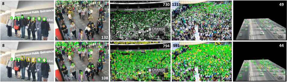
Figure 3: Examples from WiderFace, SHB, UCF, SHA, and TRANCOS datasets. The top row is test images with ground truth (bounding boxes or dots) while the bottom row is our detection. The numbers in images denote the ground truth and estimated counts, respectively. The green bounding boxes denote good detection while the yellows are not according to our evaluation protocol.

4.4 Counting

ShanghaiTech  We first present an ablation study of PSDDN and then compare it with state-of-the-art.

Ablation study. We present several variants (Pv0-Pv3) of PSDDN by gradually adding the proposed elements into the network. Referring to Sec. 3, we denote by Pv0 the model trained in a fully-supervised way using the fixed pseudo ground truth initialization and classic bounding-box regression as in [32]; Pv1: the pseudo ground truth in Pv0 is iteratively updated; Pv2: the classic bounding box regression in Pv1 is upgraded to our new way; Pv3 (PSDDN): the curriculum learning strategy is adopted in Pv2.

The result is presented in Table 1 on both SHA and SHB. We take SHA as an example: the MAE for Pv0 starts from 168.6; it decreases to 104.7 for Pv1 and 89.8 for Pv2, respectively; finally, it reaches the lowest MAE 85.4 for Pv3, which is the full version of PSDDN. In the meantime, the MSE also significantly decreases from 268.3 of Pv0 to 159.2 of Pv3. We notice that the same observation goes with SHB as well. The result shows that each component of PSDDN provides a clear benefit in the overall system.

Dataset	SHA		SHB
Measures	MAE	MSE	MAE	MSE
Pv0	168.6	268.3	69.8	98.1
Pv1	104.7	193.8	41.7	66.6
Pv2	89.8	169.5	19.1	42.4
Pv3(PSDDN)	85.4	159.2	16.1	27.9
PSDDN + [20]	65.9	112.3	9.1	14.2
Li et al. [20]	68.2	115.0	10.6	16.0
Ranjan et al. [31]	68.5	116.2	10.7	16.0
Liu et al. [24]	73.6	112.0	13.7	21.4
Liu et al. [22]	-	-	20.7	29.4
DetNet in [22]	-	-	44.9	73.2
Sindagi et al. [41]	73.6	106.4	20.1	30.1
Sam et al. [35]	90.4	135.0	21.6	33.4

Table 1: Crowd counting: ablation study of PSDDN (Pv0-Pv3 denote different variants of PSDDN) and its comparison with state-of-the-art on ShanghaiTech dataset.

Comparison with state-of-the-art. We compare our work with prior arts [20, 31, 24, 22, 41, 35]. It can be seen that our detection-based method PSDDN already performs close to recent density-based methods. Furthermore, by combing our PSDDN result with [20] using the attention module in [22] we show that the obtained result outperforms the state-of-the-art. For instance, on SHA, PSDDN + [20] produces MAE 65.9 on SHA and 9.1 on SHB. We notice two things: 1) we can obtain better counting results by adjusting the detection confidence scores; on the contrary, we fix it with a high value (0.8) for all datasets to guarantee that the predictions are reliable at every local position; 2) the regression-based methods sometimes produce bad results in some local area of the image, which can not be reflected in the MAE metric; there is another metric called GAME [10] which is able to overcome this limitation. We will discuss later in TRANCOS dataset to show that our detection-based method is much better in the GAME metric. We show some examples of PSDDN in Fig. 3.

The notation “DetNet” for [22] denotes the counting-by-detection result in it, where they annotate on partial of the bounding boxes in SHB and train a fully-supervised Faster R-CNN detector. PSDDN clearly outperforms the DetNet results. But we do not claim that point (weakly)-supervised learning is normally better than fully-supervised learning. Specifically for DetNet, they did not employ any of the data augmentation tricks as in PSDDN. The main limitation for fully-supervised detection methods in crowd counting lies in the large amount of bounding box annotations required. It can be unrealistic in very dense crowds. Our PSDDN instead provides an alternative way to conduct counting-by-detection with only point supervision; it performs very well in the evaluation of both counting and detection.

UCF_CC_50  It has the densest crowds so far in crowd counting task. We show in Table 2 that our PSDDN can still produce competitive result: the MAE is 359.4 while the MSE is 514.8. In the detection session, we will show that despite the tiny heads in UCF, PSDDN is still able to produce reasonable bounding boxes on them (Fig. 3: third column).

Counting	UCF
Measures	MAE	MSE	AP
Li et al. [20]	266.1	397.5	-
Liu et al. [24]	279.6	388.9	-
Sindagi et al. [41]	295.8	320.9	-
Sam et al. [35]	318.1	439.2	-
PSDDN	359.4	514.8	0.536

Table 2: Comparison of PSDDN with state-of-the-art on UCF dataset. MAE, MSE are reported for crowd counting while AP is reported for person detection.

4.5 Detection

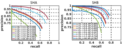
Figure 4: Precision-recall curves with different $c$ and $r$.

ShanghaiTech  In Fig. 4, we first present the precision-recall curves of different $c$ and $r$ (see Sec. 4.3) on SHA and SHB. The recall rates of different curves stop at some points as we fix the confidence score in the detection output. When we fix $r$, the AP improves with an increase of $c$; $c$ is chosen by default as 20 to apply a hard constraint on the center distance between the prediction and ground truth. On the other hand, when we fix $c$, the AP improves with an increase of $r$. As mentioned in Sec. 4.3, the crowds in SHA are much denser than in SHB, we choose by default $r=1.2$ for SHA and $r=0.8$ for SHB. We also present the result of $r=\infty$ which only cares the head center localizations (like in [18, 14]): we get very good AP 0.737 and 0.759 for SHA and SHB, respectively. [18, 14] did not present localization results in ShanghaiTech, we can not directly compare with them. But simply localizing the head centers is not enough for a detection task, we will further discuss in the WiderFace dataset where we have the real ground truth bounding boxes for evaluation.

Following the counting experiment, we also present the ablation study of PSDDN in detection. The result is shown in Table 3: the AP on SHA is significantly increased from 0.308 for Pv0 to 0.554 for Pv3; the same goes for SHB, where the AP is increased from 0.015 to 0.663 eventually. We notice we also tried to train a Faster R-CNN [32] using the fixed pseudo ground truth, which is as low as in Pv0.

Dataset	Pv0	Pv1	Pv2	Pv3 (PSDDN)
SHA	0.308	0.491	0.539	0.554
SHB	0.015	0.241	0.582	0.663

Table 3: Person detection: ablation study of PSDDN on ShanghaiTech (SHA and SHB) dataset. AP is reported.

Methods	Annotations	WiderFace
		easy	medium	hard
Avg. BB	points(test)+ mean size	0.002	0.083	0.059
FR-CNN (ps)	points(train) + mean size	0.008	0.183	0.108
FR-CNN (fs)	bounding boxes (train)	0.840	0.724	0.347
PSDDN	points(train)	0.605	0.605	0.396

Table 4: Person detection on WiderFace. “Annotations” denotes different levels of annotations employed in the methods. “mean size” refers to the mean ground truth bounding box size over the training set while “point(test)” specifically denotes that the bounding box centers are known for test. Avg. BB adds bounding boxes at each test point using the mean size. FR-CNN: Faster R-CNN.

UCF_CC_50  Table 2 shows the detection performance of PSDDN on UCF. In this dataset with very dense crowds, our method still achieves the AP of 0.536. An example is shown in Fig. 3: third column. We refer the readers to those people sitting in the upper balcony (e.g. yellow ones): they are not annotated as ground truth but detected by PSDDN.

WiderFace   WiderFace is a face detection dataset, its crowd density is less denser than that in a typical crowd counting dataset; we report results in Table 4 to show the generalizability of our method. It can be seen using only point-level annotations PSDDN still manages to achieve AP 0.605, 0.605, 0.396 on the easy, medium, and hard set.

Comparison to others. Since we have the bounding box annotations available for both training and test in WiderFace, we try to compare PSDDN with [18, 14, 22]. [18, 14] predicts either localization maps or segmentation blobs for both object localization and crowd counting. Predicting the exact size and shape of the object is not considered necessary for crowd counting in their works. However, we argue that it is important to object recognition and tracking. We assume there exists another method that can correctly localize every head center at test (better than any of [18, 14]), bounding boxes are added in a post-processing way using the mean ground truth size from the training set. It is denoted as Avg.BB in Table 4. The results are very low. We notice that we also tried to add the boxes in a similar way to our pseudo ground truth initialization at each test point, the APs are also very low. This demonstrates that it is not straightforward to add bounding boxes on top of the head point localization results. We also compare PSDDN with Faster R-CNN [32] using two different levels of annotations in Table 4: FR-CNN(ps) and FR-CNN(fs). First, we use the head point annotations together with the mean ground truth size to generate bounding boxes for training; it performs much worse than our PSDDN. Next, we follow [15] to use the manually annotated bounding boxes to train Faster R-CNN, which is analogue to the DetNet in [22]. PSDDN performs lower AP than FR-CNN(fs) on the easy and medium set but higher AP on the hard set. We point out that, many faces are well covered by the detection of PSDDN but not taken as good ones (yellow ones in Fig. 3: first column) only because of their low IoU with the annotated ground truth. We believe this has displayed some potential for future improvement.

TRANCOS  We evaluate PSDDN on TRANCOS dataset to test its generalizability, though it is proposed for person detection and counting. The Grid Average Absolute Error (GAME) is used to evaluate the counting performance. We refer the readers to [20, 10] for the definition of GAME(L) with different levels of $L$. For a specific $L$, GAME(L) subdivides the image using a grid of $4^{L}$ non-overlapping regions, and the error is computed as the sum of the mean absolute errors in each of these regions. When L = 0, the GAME is equivalent to the MAE metric. We present the result of our PSDDN in Table 5 where we obtain 4.79, 5.43, 6.68 and 8.40 for GAME0, GAME1, GAME2 and GAME3, respectively. Comparing our method with the state-of-the-art, PSDDN outperforms the best regression-based method [20] on GAME1, GAME2 and GAME3 and is competitive with it on GAME0. Unsurprisingly, the GAME theory is designed to penalize those predictions with a good MAE but a wrong localization of the objects. Our method produces good results on both overall vehicle counting and local vehicle localization/detection. The AP result of PSDDN for detection is 0.669 with $r=1$.

Methods	GAME0	GAME1	GAME2	GAME3	AP
Victor et al. [19]	13.76	16.72	20.72	24.36	-
Onoro et al. [27]	10.99	13.75	16.09	19.32	-
Li et al. [20]	3.56	5.49	8.57	15.04	-
PSDDN	4.79	5.43	6.68	8.40	0.669

Table 5: Results on TRANCOS dataset.

5 Conclusion

In this paper we propose a point-supervised deep detection network for person detection and counting in crowds. Pseudo ground truth bounding boxes are firstly initialized from the head point annotations, and updated iteratively during the training. Bounding box regression is conducted in a way to compare each predicted box with the ground truth boxes within a local band area. A curriculum learning strategy is introduced in the end to cope with the density variation in the training set. Thorough experiments have been conducted on several standard benchmarks to show the efficiency and effectiveness of PSDDN on both person detection and crowd counting. Future work will be focused on further reducing the supervision in this task.

Acknowledgments. This work was supported by National Key Research and Development Program of China (2017YFB0802300), National Natural Science Foundation of China (61828602 and 61773270).

References

- [1] Yancheng Bai, Yongqiang Zhang, Mingli Ding, and Bernard Ghanem. Finding tiny faces in the wild with generative adversarial network. In CVPR, 2018.
- [2] Amy Bearman, Olga Russakovsky, Vittorio Ferrari, and Li Fei-Fei. What’s the point: Semantic segmentation with point supervision. In ECCV, 2016.
- [3] Yoshua Bengio, Jérôme Louradour, Ronan Collobert, and Jason Weston. Curriculum learning. In ICML, 2009.
- [4] Steve Branson, Pietro Perona, and Serge Belongie. Strong supervision from weak annotation: Interactive training of deformable part models. In ICCV, 2011.
- [5] Gabriel J Brostow and Roberto Cipolla. Unsupervised bayesian detection of independent motion in crowds. In CVPR, 2006.
- [6] Antoni B Chan, Zhang-Sheng John Liang, and Nuno Vasconcelos. Privacy preserving crowd monitoring: Counting people without people models or tracking. In CVPR, 2008.
- [7] Antoni B Chan and Nuno Vasconcelos. Bayesian poisson regression for crowd counting. In ICCV, 2009.
- [8] Ross Girshick. Fast r-cnn. In ICCV, 2015.
- [9] Ross Girshick, Jeff Donahue, Trevor Darrell, and Jitendra Malik. Rich feature hierarchies for accurate object detection and semantic segmentation. In CVPR, 2014.
- [10] Ricardo Guerrero-Gómez-Olmedo, Beatriz Torre-Jiménez, Roberto López-Sastre, Saturnino Maldonado-Bascón, and Daniel Onoro-Rubio. Extremely overlapping vehicle counting. In Iberian Conference on Pattern Recognition and Image Analysis, 2015.
- [11] Kaiming He, Xiangyu Zhang, Shaoqing Ren, and Jian Sun. Deep residual learning for image recognition. In CVPR, pages 770–778, 2016.
- [12] Peiyun Hu and Deva Ramanan. Finding tiny faces. In CVPR, 2017.
- [13] Haroon Idrees, Imran Saleemi, Cody Seibert, and Mubarak Shah. Multi-source multi-scale counting in extremely dense crowd images. In CVPR, 2013.
- [14] Haroon Idrees, Muhmmad Tayyab, Kishan Athrey, Dong Zhang, Somaya Al-Maadeed, Nasir Rajpoot, and Mubarak Shah. Composition loss for counting, density map estimation and localization in dense crowds. In ECCV, 2018.
- [15] Huaizu Jiang and Erik Learned-Miller. Face detection with the faster r-cnn. In International Conference on Automatic Face & Gesture Recognition (FG), 2017.
- [16] Sam Johnson and Mark Everingham. Clustered pose and nonlinear appearance models for human pose estimation. 2010.
- [17] Alex Krizhevsky, Ilya Sutskever, and Geoffrey E Hinton. Imagenet classification with deep convolutional neural networks. In NIPS, 2012.
- [18] Issam H Laradji, Negar Rostamzadeh, Pedro O Pinheiro, David Vazquez, and Mark Schmidt. Where are the blobs: Counting by localization with point supervision. In ECCV, 2018.
- [19] Victor Lempitsky and Andrew Zisserman. Learning to count objects in images. In NIPS, 2010.
- [20] Yuhong Li, Xiaofan Zhang, and Deming Chen. Csrnet: Dilated convolutional neural networks for understanding the highly congested scenes. In CVPR, 2018.
- [21] Shengcai Liao, Yang Hu, Xiangyu Zhu, and Stan Z Li. Person re-identification by local maximal occurrence representation and metric learning. In CVPR, 2015.
- [22] Jiang Liu, Chenqiang Gao, Deyu Meng, and Alexander G. Hauptmann. Decidenet: Counting varying density crowds through attention guided detection and density estimation. In CVPR, 2018.
- [23] Wei Liu, Dragomir Anguelov, Dumitru Erhan, Christian Szegedy, Scott Reed, Cheng-Yang Fu, and Alexander C Berg. Ssd: Single shot multibox detector. In ECCV, 2016.
- [24] Xialei Liu, Joost Weijer, and Andrew D Bagdanov. Leveraging unlabeled data for crowd counting by learning to rank. In CVPR, 2018.
- [25] Zhang Lu, Miaojing Shi, and Qiaobo Chen. Crowd counting via scale-adaptive convolutional neural network. In WACV, 2018.
- [26] Mahyar Najibi, Pouya Samangouei, Rama Chellappa, and Larry S Davis. Ssh: Single stage headless face detector. In ICCV, 2017.
- [27] Daniel Onoro-Rubio and Roberto J López-Sastre. Towards perspective-free object counting with deep learning. In ECCV, 2016.
- [28] Dim P Papadopoulos, Jasper RR Uijlings, Frank Keller, and Vittorio Ferrari. Extreme clicking for efficient object annotation. In ICCV, pages 4940–4949, 2017.
- [29] Vincent Rabaud and Serge Belongie. Counting crowded moving objects. In CVPR, 2006.
- [30] Deva Ramanan. Learning to parse images of articulated bodies. In NIPS, 2007.
- [31] Viresh Ranjan, Hieu Le, and Minh Hoai. Iterative crowd counting. In ECCV, 2018.
- [32] Shaoqing Ren, Kaiming He, Ross Girshick, and Jian Sun. Faster r-cnn: Towards real-time object detection with region proposal networks. In NIPS, 2015.
- [33] Mikel Rodriguez, Ivan Laptev, Josef Sivic, and Jean-Yves Audibert. Density-aware person detection and tracking in crowds. In ICCV, 2011.
- [34] Olaf Ronneberger, Philipp Fischer, and Thomas Brox. U-net: Convolutional networks for biomedical image segmentation. In MICCAI, 2015.
- [35] Deepak Babu Sam, Shiv Surya, and R Venkatesh Babu. Switching convolutional neural network for crowd counting. In CVPR, 2017.
- [36] Ben Sapp and Ben Taskar. Modec: Multimodal decomposable models for human pose estimation. In CVPR, 2013.
- [37] Florian Schroff, Dmitry Kalenichenko, and James Philbin. Facenet: A unified embedding for face recognition and clustering. In CVPR, 2015.
- [38] Miaojing Shi and Vittorio Ferrari. Weakly supervised object localization using size estimates. In ECCV, 2016.
- [39] Miaojing Shi, Zhaohui Yang, Chao Xu, and Qijun Chen. Revisiting perspective information for efficient crowd counting. In CVPR, 2019.
- [40] Abhinav Shrivastava, Abhinav Gupta, and Ross Girshick. Training region-based object detectors with online hard example mining. In CVPR, 2016.
- [41] Vishwanath A Sindagi and Vishal M Patel. Generating high-quality crowd density maps using contextual pyramid cnns. In ICCV, 2017.
- [42] Russell Stewart, Mykhaylo Andriluka, and Andrew Y Ng. End-to-end people detection in crowded scenes. In CVPR, 2016.
- [43] Paul Viola, Michael J Jones, and Daniel Snow. Detecting pedestrians using patterns of motion and appearance. IJCV, 63(2):153–161, 2003.
- [44] Catherine Wah, Steve Branson, Pietro Perona, and Serge Belongie. Multiclass recognition and part localization with humans in the loop. In ICCV, 2011.
- [45] Tinghuai Wang, Bo Han, and John Collomosse. Touchcut: Fast image and video segmentation using single-touch interaction. Computer Vision and Image Understanding, 120:14–30, 2014.
- [46] Shuo Yang, Ping Luo, Chen-Change Loy, and Xiaoou Tang. Wider face: A face detection benchmark. In CVPR, pages 5525–5533, 2016.
- [47] Cong Zhang, Hongsheng Li, Xiaogang Wang, and Xiaokang Yang. Cross-scene crowd counting via deep convolutional neural networks. In CVPR, 2015.
- [48] Xiaopeng Zhang, Jiashi Feng, Hongkai Xiong, and Qi Tian. Zigzag learning for weakly supervised object detection. In CVPR, 2018.
- [49] Yingying Zhang, Desen Zhou, Siqin Chen, Shenghua Gao, and Yi Ma. Single-image crowd counting via multi-column convolutional neural network. In CVPR, 2016.