Ultracold homonuclear and heteronuclear collisions in metastable helium

Abstract

Scattering and ionizing cross sections and rates are calculated for ultracold collisions between metastable helium atoms using a fully quantum-mechanical close-coupled formalism. Homonuclear collisions of the bosonic ⁴He${}^{*}+{}^{4}$He^∗ and fermionic ³He${}^{*}+{}^{3}$He^∗ systems, and heteronuclear collisions of the mixed ³He${}^{*}+{}^{4}$He^∗ system, are investigated over a temperature range 1 $\mu$K to 1 K. Carefully constructed Born-Oppenheimer molecular potentials are used to describe the electrostatic interaction between the colliding atoms, and complex optical potentials used to represent loss through ionization from the ${}^{1,3}\Sigma$ states. Magnetic spin-dipole mediated transitions from the ${}^{5}\Sigma$ state are included and results reported for spin-polarized and unpolarized systems. Comparisons are made with experimental results, previous semi-classical models, and a perturbed single channel model.

I Introduction

Knowledge of the dynamics of ultracold collisions in dilute quantum gases is crucial to the understanding of the cooling and trapping of these gases. The precision and control of these gases allows for the investigation of many-body phenomena in quantum degenerate gases Bloch2008 such as quantized vortices Tsubota2013 and topological states in optical lattices Cooper2019 . Metastable rare gases are of particular interest as the release of the large internal energy can be used by experimentalists to easily detect individual events with high resolution using a microchannel plate and to potentially count each atom which has been ionized or has escaped from the trap Vassen2012 .

Metastable helium is an attractive prospect for experimental and theoretical studies of fundamental aspects of ultracold collisions because it has only one active electron, accurate molecular potentials exist to represent the interaction between the colliding atoms, and large numbers ($\gtrsim 10^{8}$) of both the bosonic ⁴He${}^{*}\equiv{}^{4}$He(1s2s ³S₁) and fermionic ³He${}^{*}\equiv{}^{3}$He(1s2s ³S₁) isotopes can be trapped Stas2004 , allowing the investigation of the effects of different atomic structures and quantum statistical symmetries. Previous studies have successfully demonstrated the Hanbury-Brown-Twiss effect for both fermionic and bosonic degenerate gases Jeltes2007 , ghost imaging with correlated atom pairs Khakimov2016 and have tested quantum electrodynamic calculations through precise tune-out wavelength measurement Henson2015 .

The ionizing processes

$$\mathrm{He}^{*}+\mathrm{He}^{*}=\left\{\begin{array}[]{ll}\mathrm{He}+\mathrm{He}^{+}+e^{-},&(\mathrm{PI})\\ \mathrm{He}^{+}_{2}+e^{-},&(\mathrm{AI})\end{array}\right.$$ (1)

where PI stands for Penning ionization and AI for associative ionization, are an important source of loss of trapped atoms. As the detailed mechanisms involved are not important in the present study we shall use PI to denote both processes.

As the ³He^∗ and ⁴He^∗ metastable atoms both have an electronic spin of $s=1$, these ionization processes are suppressed for an incoming state with total spin $S=2$ since they would violate spin conservation. The very weak spin-dipole magnetic interaction can produce spin flips and mediate PI in collisions with $S=2$ but the corresponding ionization rate is four orders of magnitude less than that for collisions with $S=0$ or $S=1$ for which the total electronic spin is conserved Venturi2000 ; Sirjean2002 .

Homonuclear ionizing collisions of the bosonic ⁴He${}^{*}+{}^{4}$He^∗ system have been investigated experimentally by Mastwijk et al. Mastwijk1998 , Tol et al. Tol1999 , Kumakura and Morita KM1999 , and Stas et al. Stas2006 . The measured unpolarized ionization rates $K({}^{4}\text{He})$ differed significantly between the various groups. Kumakura and Morita KM1999 , and Stas et al. Stas2006 have also studied collisions in the fermionic ³He${}^{*}+{}^{3}$He^∗ system but their measured rates $K({}^{3}\text{He})$ differ widely. Both Kumakura and Morita KM1999 , and Stas et al. Stas2006 , proposed simple semi-classical models in which the inelastic scattering is viewed as a two-stage process of scattering from the molecular potential $V(R)$ at large internuclear distance ($R\gtrsim 100\,a_{0}$) and ionization at small internuclear distance ($R\simeq 5\,a_{0}$). Since the spin-dipole interaction is ignored, the ionization probability ${}^{2S+1}P_{\text{ion}}$ is assumed to be zero for $S=2$ and is taken to be unity for $S=0,1$.

The semi-classical models differ in their calculation of the probability that the colliding atoms reach the distance at where ionization occurs. Kumakura and Morita ignore tunneling of each partial wave through its centrifugal barrier and assume the evolution of the scattering states can be approximated by an adiabatic transition in order to derive the number of accessible ionization channels. Stas et al. calculate the tunneling probabilities and find considerable quantum reflection for $s$-wave scattering, even though there is no centrifugal barrier, due to the mismatch between the large wavelength asymptotic de Broglie wave and the rapidly oscillating wave at small $R$. They also find the system is well approximated by a diabatic transition between the long-range atomic states and short-range molecular states. The two theoretical models give quite different results with the Stas et al. model in good agreement with their experimental results for ionization rates in the bosonic and fermionic systems. In section IV we will point out that considering only a two-stage process neglects an important contribution to the ionization rate and that the comparison between experiment and theory is complicated by the mixture of trapped states.

For the bosonic case a detailed theoretical study of elastic, inelastic and ionization rates using a fully quantum-mechanical close-coupling calculation already existed Venturi2000 ; Leo2001 . The ionization rates from the Stas et al. model were in moderate agreement with those of this multichannel calculation.

For the heteronuclear mixed ³He${}^{*}+{}^{4}$He^∗ system, McNamara et al. McNamara2007 have measured the ionization rate and extended the Stas et al. theoretical model to this system. They undertook a comparison of the bosonic, fermionic and mixed systems, and found the experimental results and theoretical model to be in good agreement.

The Stas et al. theoretical model has been revisited by Dickinson Dickinson2007 who showed that the stage of quantum reflection from the molecular potential can be modelled analytically for cold-atom collisions purely in terms of the long-range van der Waals coefficient and the particle masses. Ionization rates for unpolarized beams of bosonic, fermionic and mixed systems of metastable helium atoms obtained from the two models agreed well over the temperature range from 1 $\mu$K to 2 mK.

Detailed studies of ultracold collisions of metastable helium require fully quantum-mechanical methods because the onset of quantum threshold behavior cannot be described semiclassically Julienne1989 . We report here an extension of our earlier calculations for the bosonic system Venturi2000 ; Leo2001 to the fermionic and mixed systems. We calculate scattering and ionizing cross sections and rates over a temperature range 1 $\mu$K to 1 K using carefully constructed Born-Oppenheimer molecular potentials and complex optical potentials to represent loss through ionization.

The paper is organized as follows. In Sec. II the theoretical formalism describing the collisions of the metastable helium atoms is presented. The close-coupled scattering equations are derived, the molecular basis states appropriate to the various systems discussed and explicit expressions obtained for the Hamiltonian matrix elements. The calculation of cross sections and transition rate coefficients for scattering and ionizing collisions and the extraction of the required scattering matrix elements from the asymptotic solutions of the close-coupled equations are then discussed. In Sec. III we also discuss a simple perturbed single-channel model. The results of our calculations are presented and discussed in Sec. IV, and a summary of the outcomes of this investigation is given in Sec. V. Further details of the evaluation of the Hamiltonian matrix elements and the numerical solution of the multichannel equations are provided in Appendices A and B respectively.

Atomic units are used, with lengths in Bohr radii $a_{0}=0.0529177209$ nm and energies in Hartree $E_{\text{h}}=\alpha^{2}m_{e}c^{2}=27.211384$ eV.

II Theory

II.1 Multichannel equations

The total Hamiltonian for the system of two interacting metastable helium atoms $i=1,2$ with reduced mass $\mu$, interatomic separation $R$ and relative angular momentum $\hat{\mathbf{l}}$, is

$$\hat{H}=\hat{T}_{K}+\hat{H}_{\text{rot}}+\hat{H}_{\text{el}}+\hat{H}_{\text{hfs}}+\hat{H}_{\text{sd}},$$ (2)

where $\hat{T}_{K}$ is the radial kinetic energy operator

$$\hat{T}_{K}=-\frac{\hbar^{2}}{2\mu R^{2}}\frac{\partial}{\partial R}\left(R^{2}\frac{\partial}{\partial R}\right),$$ (3)

and $\hat{H}_{\text{rot}}$ is the rotational operator

$$\hat{H}_{\text{rot}}=\frac{\hat{l}^{2}}{2\mu R^{2}}.$$ (4)

The total electronic Hamiltonian is

$$\hat{H}_{\text{el}}=\hat{H}_{1}+\hat{H}_{2}+\hat{H}_{12}$$ (5)

where $\hat{H}_{i}$ is the unperturbed Hamiltonian of atom $i$ and $\hat{H}_{12}$ is the electrostatic interaction between the atoms. The term $\hat{H}_{\text{hfs}}$ describes the hyperfine structure of the ³He^∗ atom and must be included for the ³He${}^{*}+{}^{3}$He^∗ and ³He${}^{*}+{}^{4}$He^∗ systems. The spin-dipole magnetic interaction between the atoms is

$$\hat{H}_{\text{sd}}=-\frac{\xi}{\hbar^{2}R^{3}}\left[3(\hat{\mathbf{S}}_{1}\cdot\hat{\mathbf{R}})(\hat{\mathbf{S}}_{2}\cdot\hat{\mathbf{R}})-\hat{\mathbf{S}}_{1}\cdot\hat{\mathbf{S}}_{2}\right]$$ (6)

where $\hat{\mathbf{S}}_{i}$ are the electronic-spin operators, $\hat{\mathbf{R}}=\mathbf{R}/R$ is a unit vector directed along the internuclear axis, and

$$\xi=\alpha^{2}\left(\frac{\mu_{e}}{\mu_{B}}\right)^{2}\;E_{\text{h}}a_{0}^{3}.$$ (7)

Here $(\mu_{e}/\mu_{B})=1.00115965$ is the ratio of the electron magnetic moment to the Bohr magneton.

The multichannel equations describing the interacting atoms are obtained by expanding the system eigenstate $|\Psi\rangle$, which satisfies

$$\hat{H}|\Psi\rangle=E|\Psi\rangle,$$ (8)

as

$$|\Psi\rangle=\sum_{a}\frac{1}{R}G_{a}(R)|a\rangle,$$ (9)

where $G_{a}(R)$ are radial wave functions and the molecular basis is $|a\rangle=|\Phi_{a}(R,q)\rangle$, where $q$ denotes the interatomic polar coordinates $(\theta,\phi)$ and electronic coordinates $\{\mathbf{r}_{i}\}$. The state label, $a$, denotes the set of approximate quantum numbers describing the electronic-rotational states of the molecule. We make the Born-Oppenheimer (BO) approximation that the basis states $|a\rangle$ depend only parametrically on $R$ so that $\langle a^{\prime}|\hat{T}_{K}|a\rangle=0$. Forming the scalar product $\langle a^{\prime}|\hat{H}|a\rangle$ yields the set of multichannel equations

$$\sum_{a}\left[-\frac{\hbar^{2}}{2\mu}\frac{d^{2}}{dR^{2}}\delta_{a^{\prime},a}+V_{a^{\prime}a}(R)-E\delta_{a^{\prime},a}\right]G_{a}(R)=0,$$ (10)

where

$$V_{a^{\prime}a}(R)=\langle a^{\prime}|\left[\hat{H}_{\text{rot}}+\hat{H}_{\text{el}}+\hat{H}_{\text{hfs}}+\hat{H}_{\text{sd}}\right]|a\rangle.$$ (11)

II.2 Basis states and matrix elements

The molecular basis states $\{|a\rangle\}$ must be chosen such that, in the limit $R\rightarrow\infty$, they diagonalize the non-interacting two-atom system. As both ³He^∗ and ⁴He^∗ have zero orbital angular momentum and only ³He^∗ has a nuclear angular momentum $\hat{i}$, the appropriate coupling schemes are

$$\hat{\mathbf{S}}=\hat{\mathbf{S}}_{1}+\hat{\mathbf{S}}_{2}$$ (12)

for ⁴He${}^{*}+{}^{4}$He^∗,

$$\hat{\mathbf{f}}_{1}=\hat{\mathbf{S}}_{1}+\hat{\mathbf{i}}_{1},\quad\hat{\mathbf{f}}_{2}=\hat{\mathbf{S}}_{2}+\hat{\mathbf{i}}_{2},\quad\hat{\mathbf{f}}=\hat{\mathbf{f}}_{1}+\hat{\mathbf{f}}_{2}$$ (13)

for ³He${}^{*}+{}^{3}$He^∗, and

$$\hat{\mathbf{f}}_{1}=\hat{\mathbf{S}}_{1}+\hat{\mathbf{i}}_{1},\quad\hat{\mathbf{f}}=\hat{\mathbf{f}}_{1}+\hat{\mathbf{S}}_{2}$$ (14)

for ³He${}^{*}+{}^{4}$He^∗, where, in this last case, we have labelled the ³He^∗ and ⁴He^∗ atoms as atom 1 and 2 respectively. Hereafter we shall denote the three cases as 4–4, 3–3 and 3–4.

The space-fixed eigenstates for the 3–3 system are

$$|S_{1},i_{1},f_{1},S_{2},i_{2},f_{2},f,m_{f}\rangle,$$ (15)

which simplify to

$$|S_{1},i_{1},f_{1},S_{2},f,m_{f}\rangle$$ (16)

for the 3–4 system, and to

$$|S_{1},S_{2},S,M_{S}\rangle$$ (17)

for the 4–4 system. Here $m_{j}$ denotes the projection of an angular momentum $\hat{\mathbf{j}}$ onto the space-fixed $Oz$ quantization axis.

We denote these states generically by $|\Gamma,f,m_{f}\rangle$, where $\Gamma=\{\alpha_{1},\alpha_{2}\}$ and $\alpha_{i}=\{S_{i},i_{i},f_{i}\}$, with the simplifications $\alpha_{2}=S_{2}$ for the 3–4 system and, for the 4–4 system, $\alpha_{i}=S_{i}$ and $(f,m_{f})=(S,M_{S})$. Although the desired cross sections will be expressed in terms of the states

$$|\beta\rangle\equiv|\Gamma,f,m_{f},l,m_{l}\rangle=|\Gamma,f,m_{f}\rangle|l,m_{l}\rangle,$$ (18)

where $|l,m_{l}\rangle$ are the relative motion eigenstates, it is more convenient to perform the calculations with the coupled states

$$|\Gamma,f,l,J,M_{J}\rangle=\sum_{m_{f},m_{l}}C^{flJ}_{m_{f}m_{l}M_{J}}|\Gamma,f,m_{f}\rangle|l,m_{l}\rangle,$$ (19)

where $\hat{\mathbf{J}}=\hat{\mathbf{f}}+\hat{\mathbf{l}}$ is the total angular momentum. This simplifies the calculations as $J$ and $M_{J}$ are conserved and fewer coupled equations are required since they are independent of $M_{J}$. In (19) $C^{{\,j_{1}}{\,j_{2}}{\,j}}_{{\,m_{1}}{\,m_{2}}{\,m}}$ is a Clebsch-Gordan coefficient.

The states $|\Gamma,f,l,J,M_{J}\rangle$ with $i_{1}$,$i_{2}$ arbitrary are not symmetrized under $\hat{X}_{N}$, the operator that permutes the nuclear labels. We form the symmetrized states

$$|a\rangle \equiv |\Gamma;f,l,J,M_{J},X_{N}\rangle$$ (20)

$$= N_{X_{N}}\left[|a_{12}\rangle+(-1)^{X_{N}+l+f_{1}+f_{2}-f}|a_{21}\rangle\right],$$

where

$$|a_{12}\rangle=|\left(\alpha_{1}\right)_{A},\left(\alpha_{2}\right)_{B},f,l,J,M_{J}\rangle,$$ (21)

and

$$|a_{21}\rangle=|\left(\alpha_{2}\right)_{A},\left(\alpha_{1}\right)_{B},f,l,J,M_{J}\rangle.$$ (22)

Here, the subscripts $A$ and $B$ indicate the labelling of the nuclei, the normalization constant is $N_{X_{N}}=1/\sqrt{2(1+\delta_{\alpha_{1},\alpha_{2}})}$, and $X_{N}=0(1)$ for bosonic (fermionic) systems. This gives the selection rule $(-1)^{l-S}=1$ for the 4–4 system and $(-1)^{l+f_{1}+f_{2}-f}=1$ for the 3–3 system. For the 3–4 system, the symmetrized states present no advantage and so we work in the unsymmetrized basis, with $i_{1}=\frac{1}{2}$ and $i_{2}=0$. We note that, in the case of the 4–4 system, the selection rule also enforces a symmetry of $l$ even (odd) for gerade (ungerade) states when considering the symmetry under electronic inversion.

The multichannel equations (10) require the matrix elements of $\hat{H}_{\text{rot}}$, $\hat{H}_{\text{el}}$, $\hat{H}_{\text{hfs}}$ and $\hat{H}_{\text{sd}}$ in the basis $|a\rangle$. The rotation matrix elements are simply

$$\langle a^{\prime}|\hat{H}_{\text{rot}}|a\rangle=\frac{\langle a^{\prime}|\hat{l}^{2}|a\rangle}{2\mu R^{2}}=\delta_{a,a^{\prime}}\frac{l(l+1)\hbar^{2}}{2\mu R^{2}}.$$ (23)

The eigenstates of $\hat{H}_{\mathrm{el}}$ are the body-fixed states arising from the coupling $\hat{\mathbf{S}}=\hat{\mathbf{S}}_{1}+\hat{\mathbf{S}}_{2}$ and must also be eigenstates of the electron inversion operator $\hat{P}_{S}$. They satisfy

$$\hat{H}_{\text{el}}|\left(S_{1}\right)_{A},\left(S_{2}\right)_{B},S,\Omega_{S},w\rangle={}^{2S+1}V_{\Sigma_{w}}(R)$$

$$\times|\left(S_{1}\right)_{A},\left(S_{2}\right)_{B},S,\Omega_{S},w\rangle$$ (24)

where $\Omega_{S}$ denotes the projection of $\hat{\mathbf{S}}$ onto the internuclear axis $\mathbf{R}$, ${}^{2S+1}V_{\Sigma_{w}}(R)$ are the Born-Oppenheimer molecular potentials, and $w=0(1)$ for gerade (ungerade) symmetry. The related space-fixed states

$$|\left(S_{1}\right)_{A},\left(S_{2}\right)_{B},S,M_{S},w\rangle=\sum_{\Omega_{S}}D^{S}_{\Omega_{S},M_{S}}(\phi,\theta,0)$$

$$\times|\left(S_{1}\right)_{A},\left(S_{2}\right)_{B},S,\Omega_{S},w\rangle,$$ (25)

where $D^{S}_{\Omega_{S},M_{S}}(\phi,\theta,0)$ is the Wigner rotation matrix, are also eigenstates of $\hat{H}_{\text{el}}$, satisfying (II.2), as the Born-Oppenheimer potentials are independent of $\Omega_{S}$. We note that these states $|\left(S_{1}\right)_{A},\left(S_{2}\right)_{B},S,M_{S},w\rangle$ are also eigenstates of $\hat{P}_{S}$ and are gerade (ungerade) for even (odd) $S$. Hereafter we shall omit the label $w$ on the potentials. The matrix elements $\langle a^{\prime}|\hat{H}_{\text{el}}|a\rangle$ are constructed from the matrix elements Cocks2015 (see Appendix A)

$$\langle a_{12}^{\prime}|\hat{H}_{\text{el}}|a_{12}\rangle = \delta_{\eta^{\prime},\eta}[f_{1}^{\prime}f_{2}^{\prime}f_{1}f_{2}]^{1/2}\;\sum_{S,i}[Si]$$

$$\times\left\{\begin{matrix}{S_{1}}&{\!\!\!S_{2}}&{\!\!\!S}\cr{i_{1}}&{\!\!\!i_{2}}&{\!\!\!i}\cr{f_{1}^{\prime}}&{\!\!\!f_{2}^{\prime}}&{\!\!\!f}\cr\end{matrix}\right\}\left\{\begin{matrix}{S_{1}}&{\!\!\!S_{2}}&{\!\!\!S}\cr{i_{1}}&{\!\!\!i_{2}}&{\!\!\!i}\cr{f_{1}}&{\!\!\!f_{2}}&{\!\!\!f}\cr\end{matrix}\right\}{}^{2S+1}V_{\Sigma}(R),$$

and the elements $\langle a_{21}^{\prime}|\hat{H}_{\text{el}}|a_{21}\rangle$ and $\langle a_{21}^{\prime}|\hat{H}_{\text{el}}|a_{12}\rangle$ which are obtained from (II.2) by the obvious replacements. Here $[ab\ldots]=(2a+1)(2b+1)\ldots$, the notation $\left\{\begin{matrix}{a}&{\!\!\!b}&{\!\!\!c}\cr{d}&{\!\!\!e}&{\!\!\!f}\cr{g}&{\!\!\!h}&{\!\!\!i}\cr\end{matrix}\right\}$ is a Wigner 9-j symbol, and $\eta$ denotes the set of quantum numbers $\{S_{1},i_{1},S_{2},i_{2},f,l,J,M_{J}\}$. For the 3–4 system, $i_{2}=0$, $f_{2}=f_{2}^{\prime}=S_{2}$ and (II.2) simplifies to

$$\langle a_{12}^{\prime}|\hat{H}_{\text{el}}|a_{12}\rangle = \delta_{\xi^{\prime},\xi}(-1)^{f_{1}-f_{1}^{\prime}}[f_{1}^{\prime}f_{1}]^{1/2}\sum_{S}[S]$$

$$\times\left\{\begin{matrix}{S_{1}}&{\!\!\!S_{2}}&{\!\!\!S}\cr{f}&{\!\!\!i_{1}}&{\!\!\!f_{1}^{\prime}}\cr\end{matrix}\right\}\left\{\begin{matrix}{S_{1}}&{\!\!\!S_{2}}&{\!\!\!S}\cr{f}&{\!\!\!i_{1}}&{\!\!\!f_{1}}\cr\end{matrix}\right\}{}^{2S+1}V_{\Sigma}(R),$$

where $\left\{\begin{matrix}{a}&{\!\!\!b}&{\!\!\!c}\cr{d}&{\!\!\!e}&{\!\!\!f}\cr\end{matrix}\right\}$ is a 6-j symbol and $\xi$ denotes the set $\{S_{1},i_{1},S_{2},f,l,J,M_{J}\}$. Further simplification occurs for the 4–4 system. With $i_{1}=0,f_{1}=f_{1}^{\prime}=S_{1},f=S$, (II.2) reduces to

$$\langle a_{12}^{\prime}|\hat{H}_{\text{el}}|a_{12}\rangle=\delta_{\rho^{\prime},\rho}{}^{2S+1}V_{\Sigma}(R),$$ (28)

where $\rho=\{\alpha_{1},\alpha_{2},f,l,J,M_{J}\}$. Note that, for the 3–3 and 3–4 systems, $\hat{H}_{\text{el}}$ couples the different hyperfine levels $f_{i}$.

The matrix elements of $\hat{H}_{\text{hfs}}$ are assumed to be independent of the interatomic spacing, such that $\hat{H}_{\text{hfs}}=\hat{H}_{\text{hfs,1}}+\hat{H}_{\text{hfs,2}}$, where the individual atomic hyperfine splitting matrix elements are independent of $m_{f_{i}}$ and are given by

$$\langle\alpha_{i}^{\prime}|\hat{H}_{\text{hfs,i}}|\alpha_{i}\rangle=\delta_{\alpha_{i}^{\prime},\alpha_{i}}E^{\text{hfs}}_{i_{i},f_{i}}.$$ (29)

For helium-4, $i_{i}=0$ and $E^{\text{hfs}}_{0,f_{i}}=0$. For helium-3 with hyperfine splitting $\epsilon_{\text{hfs}}=6739.701177$ MHz $=1.519830\times 10^{-7}\,E_{\text{h}}$ Rosner1970 , we choose our energy origin on the lower hyperfine level such that $E^{\text{hfs}}_{0.5,0.5}=\epsilon_{\text{hfs}}$ and $E^{\text{hfs}}_{0.5,1.5}=0$.

The spin-dipole interaction may be written as the scalar product of two second-rank irreducible tensors

$$\hat{H}_{\text{sd}}=V_{p}(R)\mathbf{T}^{2}\mathbf{\cdot}\mathbf{C}^{2}$$ (30)

where $\mathbf{T}^{2}$ is

$$T^{2}_{q}\equiv\left[\mathbf{S}^{1}_{1}\mathbf{\times}\mathbf{S}^{1}_{2}\right]^{2}_{q}=\sum_{\mu}C^{{\,1}{\,1}{\,2}}_{{\,\mu,}{\,q-\mu,}{\,q}}\;S^{1}_{1,\mu}S^{1}_{2,q-\mu},$$ (31)

and $\mathbf{C}^{2}$ is the second-rank tensor formed from the modified spherical harmonics

$$C^{l}_{m_{l}}(\theta,\phi)\equiv\sqrt{\frac{4\pi}{2l+1}}\;Y_{lm_{l}}(\theta,\phi)$$ (32)

where $Y_{lm_{l}}(\theta,\phi)=\langle\theta\phi|lm_{l}\rangle$. The radial factor is $V_{p}(R)=b/R^{3}$ where $b\equiv-\sqrt{6}\xi/\hbar^{2}$. The matrix elements of $\hat{H}_{\text{sd}}$ in the basis

$$|\alpha\rangle=|\left(S_{1}\right)_{A},\left(S_{2}\right)_{B},S,M_{S}\rangle|l,m_{l}\rangle,$$ (33)

are Beams2006

$$\langle\alpha^{\prime}|\hat{H}_{\text{sd}}|\alpha\rangle=V_{p}(R)D_{\alpha^{\prime}\alpha}$$ (34)

where

$$D_{\alpha^{\prime}\alpha} = \delta_{M_{S^{\prime}}+m^{\prime}_{l},M_{S}+m_{l}}\;(-1)^{M_{S^{\prime}}-M_{S}}\;C^{{\,S}{\,2}{\,S^{\prime}}}_{{\,M_{S},}{\,M_{S^{\prime}}-M_{S},}{\,M_{S^{\prime}}}}$$ (35)

$$\times C^{{\,l}{\,2}{\,l^{\prime}}}_{{\,m_{l}}{\,m^{\prime}_{l}-m_{l}}{\,m^{\prime}_{l}}}\;\langle\gamma^{\prime},S^{\prime}||\mathbf{T}^{2}||\gamma,S\rangle\langle l^{\prime}||\mathbf{C}^{2}||l\rangle$$

and $\gamma=\{S_{1},S_{2}\}$. The reduced matrix elements are given by

$$\langle\gamma^{\prime},S^{\prime}||\mathbf{T}^{2}||\gamma,S\rangle = \delta_{\gamma^{\prime},\gamma}\;\hbar^{2}\sqrt{5S_{1}(S_{1}+1)S_{2}(S_{2}+1)}$$ (36)

$$\times[S_{1}S_{2}S]^{1/2}\left\{\begin{matrix}{S_{1}}&{\!\!\!S_{2}}&{\!\!\!S}\cr{1}&{\!\!\!1}&{\!\!\!2}\cr{S_{1}}&{\!\!\!S_{2}}&{\!\!\!S^{\prime}}\cr\end{matrix}\right\}$$

and

$$\langle l^{\prime}||\mathbf{C}^{2}||l\rangle=\left[\frac{2l+1}{2l^{\prime}+1}\right]^{\frac{1}{2}}\;C^{{\,l}{\,2}{\,l^{\prime}}}_{{\,0}{\,0}{\,0}}.$$ (37)

The nonzero reduced matrix elements are $\langle\gamma^{\prime},2||\mathbf{T}^{2}||\gamma,2\rangle=\delta_{\gamma^{\prime},\gamma}\hbar^{2}\sqrt{7/3}$, $\langle\gamma^{\prime},0||\mathbf{T}^{2}||\gamma,2\rangle=-\delta_{\gamma^{\prime},\gamma}\hbar^{2}\sqrt{5/3}$, and $\langle\gamma^{\prime},1||\mathbf{T}^{2}||\gamma,1\rangle=\delta_{\gamma^{\prime},\gamma}\hbar^{2}\sqrt{5/3}$.

The conversion from the $|\alpha\rangle$ basis to the $|a_{12}\rangle$ basis gives (see Appendix A)

$$\langle a_{12}^{\prime}|\hat{H}_{\mathrm{sd}}|a_{12}\rangle=V_{p}(R)D_{a_{12}^{\prime}a_{12}}$$ (38)

where

$$D_{a_{12}^{\prime}a_{12}} = \delta_{\lambda^{\prime},\lambda}(-1)^{l^{\prime}+J}[f_{1}^{\prime}f_{2}^{\prime}f^{\prime}f_{1}f_{2}fl^{\prime}]^{1/2}\langle l^{\prime}||\mathbf{C}^{2}||l\rangle$$ (39)

$$\times\left\{\begin{matrix}{f}&{\!\!\!2}&{\!\!\!f^{\prime}}\cr{l^{\prime}}&{\!\!\!J}&{\!\!\!l}\cr\end{matrix}\right\}\sum_{S^{\prime},S,i}(-1)^{-S^{\prime}-i}[S^{\prime}i][S]^{1/2}$$

$$\times\left\{\begin{matrix}{f}&{\!\!\!2}&{\!\!\!f^{\prime}}\cr{S^{\prime}}&{\!\!\!i}&{\!\!\!S}\cr\end{matrix}\right\}\langle\gamma^{\prime},S^{\prime}||\mathbf{T}^{2}||\gamma,S\rangle$$

$$\times\left\{\begin{matrix}{S_{1}}&{\!\!\!S_{2}}&{\!\!\!S^{\prime}}\cr{i_{1}}&{\!\!\!i_{2}}&{\!\!\!i}\cr{f_{1}^{\prime}}&{\!\!\!f_{2}^{\prime}}&{\!\!\!f^{\prime}}\cr\end{matrix}\right\}\left\{\begin{matrix}{S_{1}}&{\!\!\!S_{2}}&{\!\!\!S}\cr{i_{1}}&{\!\!\!i_{2}}&{\!\!\!i}\cr{f_{1}}&{\!\!\!f_{2}}&{\!\!\!f}\cr\end{matrix}\right\},$$

and $\lambda=\{S_{1},i_{1},S_{2},i_{2},J,M_{J}\}$. The elements $\langle a_{21}^{\prime}|\hat{H}_{\text{sd}}|a_{21}\rangle$ and $\langle a_{21}^{\prime}|\hat{H}_{\text{sd}}|a_{12}\rangle$ can be obtained from (39) by the obvious replacements. This expression simplifies for the 3–4 system to

$$D_{a_{12}^{\prime}a_{12}} = \delta_{\tau^{\prime},\tau}(-1)^{f_{1}-f_{1}^{\prime}+l^{\prime}+J-i_{1}}[f_{1}^{\prime}f^{\prime}f_{1}fl^{\prime}]^{1/2}\langle l^{\prime}||\mathbf{C}^{2}||l\rangle$$ (40)

$$\times\left\{\begin{matrix}{f}&{\!\!\!2}&{\!\!\!f^{\prime}}\cr{l^{\prime}}&{\!\!\!J}&{\!\!\!l}\cr\end{matrix}\right\}\sum_{S^{\prime},S}(-1)^{-S^{\prime}}[S^{\prime}][S]^{1/2}$$

$$\times\left\{\begin{matrix}{f}&{\!\!\!2}&{\!\!\!f^{\prime}}\cr{S^{\prime}}&{\!\!\!i_{1}}&{\!\!\!S}\cr\end{matrix}\right\}\langle\gamma^{\prime},S^{\prime}||\mathbf{T}^{2}||\gamma,S\rangle$$

$$\times\left\{\begin{matrix}{S_{1}}&{\!\!\!S_{2}}&{\!\!\!S^{\prime}}\cr{f^{\prime}}&{\!\!\!i_{1}}&{\!\!\!f_{1}^{\prime}}\cr\end{matrix}\right\}\left\{\begin{matrix}{S_{1}}&{\!\!\!S_{2}}&{\!\!\!S}\cr{f}&{\!\!\!i_{1}}&{\!\!\!f_{1}}\cr\end{matrix}\right\},$$

where $\tau=\{S_{1},i_{1},S_{2},J,M_{J}\}$. Finally, for the 4–4 system, we get

$$D_{a_{12}^{\prime}a_{12}} = \delta_{\omega^{\prime},\omega}(-1)^{l^{\prime}+J+S^{\prime}}[S^{\prime}l^{\prime}]^{1/2}\langle l^{\prime}||\mathbf{C}^{2}||l\rangle$$ (41)

$$\times\left\{\begin{matrix}{S}&{\!\!\!2}&{\!\!\!S^{\prime}}\cr{l^{\prime}}&{\!\!\!J}&{\!\!\!l}\cr\end{matrix}\right\}\langle\gamma^{\prime},S^{\prime}||\mathbf{T}^{2}||\gamma,S\rangle,$$

where $\omega=\{S_{1},S_{2},J,M_{J}\}$.

II.3 Cross sections

For collisions in an atom trap, the scattering cross section for transitions from an initial state $|\Gamma,f,m_{f}\rangle$ with wave number $k_{\Gamma}$ to final states $|\Gamma^{\prime},f^{\prime},m_{f}^{\prime}\rangle$ should be averaged over initial directions and integrated over all final directions Julienne1989 ; Julienne2002 , to give

$$\sigma(k_{\Gamma};\Gamma,f,m_{f}\rightarrow\Gamma^{\prime},f^{\prime},m_{f}^{\prime})=\frac{\pi N_{\Gamma}}{k^{2}_{\Gamma}}\sum_{l^{\prime},m_{l}^{\prime}}\sum_{l,m_{l}}|T_{\beta^{\prime}\beta}(E)|^{2}$$ (42)

where the factor $N_{\Gamma}=2/N_{X_{N}}^{2}=1+\delta_{\alpha_{1},\alpha_{2}}$ accounts for normalization of the incoming state, and $T_{\beta^{\prime}\beta}(E)$ are the matrix elements of the transition operator $\mathbf{T}$ between the states (18). The channel $\beta$ must be open, that is the energy $E$ of the state must be greater than the asymptotic energy $V_{\Gamma}^{\infty}\equiv E^{\mathrm{hfs}}_{i_{1}f_{1}}+E^{\mathrm{hfs}}_{i_{2}f_{2}}$ so that $k_{\Gamma}^{2}\equiv 2\mu[E-V^{\infty}_{\Gamma}]/\hbar^{2}>0$. These transition matrix elements are related to those of the total angular momentum representation (20) by

$$T_{\beta^{\prime}\beta}(E)=\sum_{J^{\prime},M_{J}^{\prime}}\sum_{J,M_{J}}C^{{\,f^{\prime}}{\,l^{\prime}}{\,J^{\prime}}}_{{\,m_{f}^{\prime}}{\,m_{l}^{\prime}}{\,M_{J}^{\prime}}}C^{{\,f}{\,l}{\,J}}_{{\,m_{f}}{\,m_{l}}{\,M_{J}}}T_{a^{\prime}a}(E).$$ (43)

This relationship simplifies as the total angular momentum transition matrix elements $T_{a^{\prime}a}(E)$ and scattering matrix elements $S_{a^{\prime}a}(E)=\delta_{a^{\prime},a}-T_{a^{\prime}a}(E)$ extracted from the asymptotic solutions of (10) are diagonal in $J$ and independent of $M_{J}$, allowing the notation $T^{J}_{\Gamma^{\prime}f^{\prime}l^{\prime},\Gamma fl}$ and $S^{J}_{\Gamma^{\prime}f^{\prime}l^{\prime},\Gamma fl}$. For the homonuclear 3–3 and 4–4 systems, the matrix elements $T_{a^{\prime}a}$ and $S_{a^{\prime}a}$ are understood to be in the symmetrized basis (19) whereas, for the heteronuclear 3–4 system, unsymmetrized states are used.

Spin-polarized systems with spin-stretched states $S=2$ for the 4–4 system, $f=3$ for the 3–3 system, and $f=\frac{5}{2}$ for the 3–4 system, are all in the $S=2$ ${}^{5}\Sigma^{+}_{g}$ state from which Penning ionization is not possible. However, the spin dipole interaction mediates transitions to the ${}^{1}\Sigma^{+}_{g}$ state from which Penning ionization is highly probable at small internuclear separations $R\lesssim 7a_{0}$. For non-spin-polarized systems with $S=0,1,2$, Penning ionization from the ${}^{3}\Sigma^{+}_{u}$ state is also highly probable at small $R$. The loss of flux due to Penning ionization can be modelled using complex optical potentials ${}^{1,3}V_{\Sigma}(R)-i{}^{1,3}\Gamma(R)/2$ where ${}^{2S+1}\Gamma(R)$ is the total autoionization width. We consider two forms of the autoionization width; a least-squares fit $\Gamma_{\text{M}}(R)$ to the tabulated values of Müller et al. Muller1991 , and the simpler form $\Gamma_{\text{GMS}}(R)=0.3\exp(-R/1.086)$ Garrison73 .

The cross section for Penning ionization requires the transition probability from the initial state $|\Gamma,f,m_{f}\rangle$ to all possible ionization channels

$$\sigma(k_{\Gamma};\Gamma,f,m_{f}\rightarrow\text{PI})=\frac{\pi N_{\Gamma}}{k_{\Gamma}^{2}}\sum_{l,m_{l}}|T(E;\beta\rightarrow\text{PI})|^{2}.$$ (44)

As the loss of flux due to coupling to these ionization channels is represented here by a complex potential, the transition matrix element for Penning ionization can be obtained from the non-unitarity of the calculated scattering matrix:

$$|S(E;\beta\rightarrow\text{PI})|^{2}=1-\sum_{\beta^{\prime}}|S_{\beta^{\prime}\beta}(E)|^{2}.$$ (45)

Experimental studies usually involve Stas2006 ; McNamara2007 unpolarized systems consisting of atoms colliding in all the possible $|\Gamma,f,m_{f}\rangle$ states. The contribution of each collision channel depends on the distribution of the magnetic substates and makes comparison of theoretical and experimental results very difficult (see sections II.4 and IV). In order to obtain some specific results, we consider an unpolarized system in which the degenerate magnetic substates $|\Gamma,f,m_{f}\rangle$ are populated according to their Boltzmann weighting factor $\exp(-V^{\infty}_{\Gamma}/k_{B}T)$, where $k_{B}$ is Boltzmann’s constant. In this distribution, states that differ only in $m_{f}$ are equally populated, hence the cross section for transitions $(\Gamma,f\rightarrow\Gamma^{\prime},f^{\prime})$, obtained by averaging (42) over $m_{f}$ and summing over $m^{\prime}_{f}$, is

$$\sigma(k_{\Gamma};\Gamma,f\rightarrow\Gamma^{\prime},f^{\prime})=\frac{\pi N_{\Gamma}}{k_{\Gamma}^{2}}\sum_{J,l^{\prime},l}\frac{2J+1}{2f+1}\;|T^{J}_{\Gamma^{\prime}f^{\prime}l^{\prime},\Gamma fl}(E)|^{2}.$$ (46)

In our calculations, we have truncated the $J$ summation at $J=20$ to achieve convergence for temperatures $T\leq 1$ K. The corresponding ionization cross section is

$$\sigma(k_{\Gamma};\Gamma,f\rightarrow\text{PI}) = \frac{1}{2f+1}\sum_{m_{f}}\sigma(k_{\Gamma};\Gamma,f,m_{f}\rightarrow\text{PI})$$ (47)

$$= \frac{\pi N_{\Gamma}}{k^{2}_{\Gamma}}\sum_{J,l}\frac{2J+1}{2f+1}$$

$$\times\left[1-\sum_{\Gamma^{\prime},f^{\prime},l^{\prime}}|S^{J}_{\Gamma^{\prime}f^{\prime}l^{\prime},\Gamma fl}(E)|^{2}\right].$$

The transition rate coefficients at temperature $T$ for each of the cross sections are

$$K(T;x\rightarrow y)=\langle\sigma(k_{\Gamma};x\rightarrow y)v\rangle$$ (48)

where $v=\hbar k_{\Gamma}/\mu$ is the relative velocity of the colliding atoms. The angle brackets denote an average over a normalized Maxwellian distribution of velocities

$$f(v)=4\pi v^{2}\left(\frac{\mu}{2\pi k_{B}T}\right)^{3/2}\exp\left(-\frac{\mu v^{2}}{2k_{B}T}\right).$$ (49)

II.4 Experimentally relevant rates

Many experiments exploit the spin-suppression of ionization in a spin-polarized cloud. In these experiments there are three major rates of interest. Foremost is the ionization rate, which is mediated by the spin-dipole interaction, and causes trap loss. This is given simply by

$$K_{\mathrm{stretched}}^{\mathrm{loss}}(T)=K(T;\Gamma,f^{\mathrm{max}},f^{\mathrm{max}}\rightarrow\mathrm{PI})$$ (50)

where $f^{\mathrm{max}}=2,\,\frac{5}{2},\,3$ for the 4–4, 3–4 and 3–3 systems, respectively. Second is the inelastic rate, also mediated by the spin-dipole interaction, which reduces the overall spin-polarization of the cloud and leads to subsequent loss. This is given by

$$K_{\mathrm{stretched}}^{\mathrm{inelastic}}(T)=\sum_{f^{\prime},m_{f}^{\prime}}K(T;\Gamma,f^{\mathrm{max}},f^{\mathrm{max}}\rightarrow\Gamma^{\prime},f^{\prime},m_{f}^{\prime}).$$ (51)

where the sum is over all combinations of $f^{\prime},m_{f}^{\prime}$ except $f^{\prime}=m_{f}^{\prime}=f^{\mathrm{max}}$. The final rate of interest is the elastic scattering rate

$$K_{\mathrm{stretched}}^{\mathrm{elastic}}(T)=K(T;\Gamma,f^{\mathrm{max}},f^{\mathrm{max}}\rightarrow\Gamma,f^{\mathrm{max}},f^{\mathrm{max}}),$$ (52)

which dominates the other rates.

In experiments that take place in a magneto-optical-trap or are otherwise in a mixture of the different atomic states, there is a wide range of different populations of the collisional states $|\Gamma,f,m_{f}\rangle$. At cold enough temperatures, we can assume that only the lowest energy hyperfine state will be occupied, although we will not make that assumption in our results. In general, there will be a spatially varying population of the magnetic sublevels, due to the laser coupling and magnetic fields applied in the trap.

As we would like to present results that are generally applicable, we choose to describe the rates in an “unpolarized” system, in which the occupancy of the atomic states is in thermal equilibrium, i.e. given by the Boltzmann factor. As this minimizes the proportion of spin-stretched collisions, we expect that an unpolarized distribution provides an upper bound to the loss rate. We want to describe the loss and thermalization rates of such an unpolarized system.

In an atomically separable basis $|\gamma_{1}\rangle|\gamma_{2}\rangle$, where $\gamma_{i}=\{S_{i},i_{i},f_{i},m_{f_{i}}\}$, the collision rate (i.e. number of collisions per unit time per volume) for loss processes is given by

$$r_{\gamma_{1},\gamma_{2}}^{\mathrm{PI}}=K(T,\gamma_{1},\gamma_{2}\rightarrow\mathrm{PI})\frac{n_{\gamma_{1}}n_{\gamma_{2}}}{1+\delta_{\gamma_{1},\gamma_{2}}}$$ (53)

where $n_{\gamma_{i}}$ is the atomic density and the denominator prevents over-counting of collision pairs for identical atoms. Analogously we have

$$r_{\zeta}^{\mathrm{PI}}=K(T;\Gamma,f,m_{f}\rightarrow\mathrm{PI})\frac{n_{\zeta}^{(2)}}{N_{\Gamma}},$$ (54)

where $\zeta\equiv\{\Gamma,f,m_{f}\}$, the 2-particle density is $n_{\zeta}^{(2)}=\sum_{\gamma_{1},\gamma_{2}}|\langle\gamma_{1},\gamma_{2}|\zeta\rangle|^{2}n_{\gamma_{1}}n_{\gamma_{2}}$, and the factor $N_{\Gamma}$ is as defined below equation (42).

With these definitions, we can show that, for an unpolarized sample, we have

$$\sum_{\zeta}r_{\zeta}^{\mathrm{PI}}=\sum_{\gamma_{1},\gamma_{2}}r_{\gamma_{1},\gamma_{2}}^{\mathrm{PI}}.$$ (55)

This allows us to introduce a total loss rate for the unpolarized system

$$\tilde{K}^{\mathrm{PI}}_{\mathrm{unpol}}(T)=\frac{1}{Z}\,\sum_{\Gamma,f}e^{-V^{\infty}_{\Gamma}/k_{B}T}(2f+1)\frac{K(T;\Gamma,f\rightarrow\text{PI})}{N_{\Gamma}},$$ (56)

where the partition function is $Z=\sum_{\Gamma,f}e^{-V^{\infty}_{\Gamma}/k_{B}T}(2f+1)$. We note that $\tilde{K}$ differs to $K$ in that the collision rate is defined purely quadratically, i.e. $r^{\mathrm{PI}}_{\mathrm{unpol}}=\tilde{K}^{\mathrm{PI}}_{\mathrm{unpol}}n^{2}$ where $n$ is the total density without any additional factor of 1/2.

In a similar fashion, we can define the thermalization collision rate, i.e. the rate of collisions which do not change the hyperfine energy of the atomic pair:

$$\tilde{K}^{\text{thermal}}_{\text{unpol}}(T)=\frac{1}{Z}\sum_{\Gamma,f,f^{\prime}}e^{-V^{\infty}_{\Gamma}/k_{B}T}(2f+1)\frac{K(T;\Gamma,f\rightarrow\Gamma,f^{\prime})}{N_{\Gamma}}.$$ (57)

II.5 Extraction of $S$-matrix elements

The $S$-matrix elements required for evaluating the cross sections (46) and (47) are determined by matching the asymptotic solutions of (10) to the combination Mies1980

$$\mathbf{G}(R)\underset{R\rightarrow\infty}{\sim}\mathbf{J}-\mathbf{N}\mathbf{K}$$ (58)

where $G_{aa^{\prime}}(R)$ is the matrix of solutions formed from $G_{a}(R)$ with the second subscript $a^{\prime}$ labelling the linearly independent solutions generated by different choices of boundary conditions. The real diagonal matrices $\mathbf{J}$ and $\mathbf{N}$ are given by

$$J_{aa} =\mathcal{C}_{\Gamma}\kappa_{\Gamma}^{1/2}Rj_{l}(k_{\Gamma}R),$$ (59)

$$N_{aa} =\mathcal{D}_{\Gamma}\kappa_{\Gamma}^{1/2}Rn_{l}(k_{\Gamma}R),$$

where $\kappa_{\Gamma}=|k_{\Gamma}|$ and $j_{l}(z)$ and $n_{l}(z)$ are the regular and irregular spherical Bessel functions. For open channels ($k_{\Gamma}^{2}>0$), the Bessel functions are oscillatory and $\mathcal{C}_{a}=\mathcal{D}_{a}=1$ and for closed channels ($k_{\Gamma}^{2}<0$) they are exponentially increasing and decreasing functions with $\mathcal{C}_{\Gamma}=(-i)^{l}$ and $\mathcal{D}_{\Gamma}=i^{l+1}$. The reactance matrix $\mathbf{K}$ is of dimension $N_{T}\times N_{T}$ where $N_{T}=N_{o}+N_{c}$ is the total number of open $N_{o}$ and closed $N_{c}$ channels.

The required open channel scattering matrix $\mathbf{S}_{oo}$ is obtained from the reactance matrix $\mathbf{K}$ by Mies1980

$$\mathbf{S}_{oo}=(\mathbf{I}+i[\mathbf{K}_{oo}+\mathbf{K}_{oo}^{R}])(\mathbf{I}-i[\mathbf{K}_{oo}+\mathbf{K}_{oo}^{R}])^{-1}$$ (60)

where

$$\mathbf{K}_{oo}^{R}=-\mathbf{K}_{oc}[\mathbf{I}+\mathbf{K}_{cc}]^{-1}\mathbf{K}_{co}$$ (61)

embodies the effects of the closed channels on $\mathbf{S}_{oo}$. The asymptotic fitting for the open channels requires very large values of $R$ where the closed channel contributions must be absent. Thus, $\mathbf{K}_{cc}\approx\mathbf{I}$, $\mathbf{K}_{oc}\approx\mathbf{0}$ and $\mathbf{K}_{oo}^{R}\approx\mathbf{0}$ so that only the open channel components of $\mathbf{K}$ are needed for the determination of $\mathbf{S}_{oo}$.

For systems formed from either ⁴He^∗, or ³He^∗ trapped in its lower hyperfine level with energy $E>V_{\Gamma}^{\infty}$, the scattering channels will be open. However, with our choice of energy origin, closed channels occur at low energies for the 3–3 and 3–4 systems. The closed channels must be included in the multichannel equations as this coupling may be quite significant at smaller values of $R$.

As a result of the complex optical potential, both $\mathbf{G}$ and $\mathbf{S}$ are complex. However, note that $\mathbf{S}$ remains symmetric.

III Perturbed single channel model

We now consider a perturbed single channel model Peach2017 for $\mathrm{He}^{*}+\mathrm{He}^{*}$ scattering in the states ${}^{1}\Sigma_{g}$, ${}^{3}\Sigma_{u}$, ${}^{5}\Sigma_{g}$. The hyperfine couplings and splittings due to the ³He^∗ nuclear spin are neglected but the constraints due to the different quantum statistical symmetries are included. If the spin dipole interaction is ignored, the radial functions $F_{kl}^{S}(R)$ for the scattering satisfy

$$\left[\frac{d^{2}}{dR^{2}}-\frac{l(l+1)}{R^{2}}-\frac{2\mu\;{}^{2S+1}V_{\Sigma}(R)}{\hbar^{2}}+k^{2}\right]F_{kl}^{S}(R)=0,$$ (62)

where $S=0,1,2$ and $k=\sqrt{2\mu E}/\hbar$. At large $R$, the radial functions have the asymptotic form (c.f. (58))

$$F_{kl}^{S}(R)\underset{R\rightarrow\infty}{\sim}\frac{1}{\sqrt{k}}\left[(kR)j_{l}(kR)\cos\eta_{l}^{S}-(kR)n_{l}(kR)\sin\eta_{l}^{S}\right].$$ (63)

The phase shifts $\eta_{l}^{S}(k)$ are complex for $S=0,1$ since ${}^{1,3}V_{\Sigma}(R)$ are complex, whereas, for $S=2$, ${}^{5}V_{\Sigma}(R)$ is real and so $\eta_{l}^{2}(k)$ is also real. The single (open) channel scattering matrix is given by

$$\mathbf{S}=\exp{[2i\eta_{l}^{S}(k)}],$$ (64)

where $|\mathbf{S}|<1$ for $S=0,1$ and $|\mathbf{S}|=1$ for $S=2$.

If we introduce the perturbation produced by the spin-dipole interaction, the channels with $S=0,2$ become coupled, whereas the states with $S=1$ give rise to a separate $S$-matrix in which the spin-dipole interaction is retained although in this case it does not affect the final collision rate very much. The scattering matrices then have the form Seaton1966

$$\mathbf{S}=e^{i\mathbf{\eta}}(\mathbf{I}+i\mathbf{K}^{\mathrm{sd}})(\mathbf{I}-i\mathbf{K}^{\mathrm{sd}})^{-1}e^{i\mathbf{\eta}},$$ (65)

where $\exp{(i\mathbf{\eta})}$ is a diagonal matrix with elements $\eta^{S}_{l}(k)$. So far no approximation has been made in writing $\mathbf{S}$ in this form.

We now use Born perturbation theory to approximate $\mathbf{K}^{\mathrm{sd}}$ by Seaton1961

$$K^{\mathrm{sd}}_{\tilde{a}^{\prime},\tilde{a}}(k)=\frac{2\mu}{\hbar^{2}}\langle\psi_{k,\tilde{a}^{\prime}}|\hat{H}_{\text{sd}}|\psi_{k,\tilde{a}}\rangle$$ (66)

where $\tilde{a}=\{\gamma,S,l,J,M_{J}\}$ and the unperturbed state eigenfunction is

$$|\psi_{k,\tilde{a}}(R)\rangle=R^{-1}F_{kl}^{S}(R)|\tilde{a}\rangle.$$ (67)

Using (38) then gives

$$K^{\mathrm{sd}}_{\tilde{a}^{\prime},\tilde{a}}(k) = -\left(\frac{2\mu}{\hbar^{2}}\right)D_{\tilde{a}^{\prime}\tilde{a}}$$ (68)

$$\times\int_{0}^{\infty}dR\;F_{kl^{\prime}}^{S^{\prime}}(R)^{*}V_{p}(R)F_{kl}^{S}(R).$$

where $D_{\tilde{a}^{\prime}\tilde{a}}$ is given by (41). In the evaluation of the radial integral any non-zero contribution from the imaginary parts of the radial functions $F_{kl^{\prime}}^{S^{\prime}}(R)$ and $F_{kl}^{S}(R)$ is neglected. This makes only a very small difference to the result for $K^{\mathrm{sd}}_{\tilde{a}^{\prime},\tilde{a}}(k)$. The $S$-matrix (65) is then evaluated without further approximation.

The elastic and ionization cross sections are given by (46) and (47) respectively, with $f=S$ and $f^{\prime}=S$.

So far we have not considered the application of this theory to the different isotopic combinations. These differences introduce changes to the interpretation of the sums over $l$ and $l^{\prime}$ where the spin-dipole interaction imposes the condition $|l-l^{\prime}|=0,2$. This interpretation depends upon the behavior of the system under $\hat{X}_{N}$ which permutes the nuclear labels, interchanging the nuclear spins and reversing the molecular axis Geltman1969 . For the bosonic 4–4 system the wavefunction must be symmetric under $\hat{X}_{N}$ and, as there is no nuclear spin, $l$ must be even (odd) for $S$ even (odd). Thus, for the ${}^{1}\Sigma_{g}$ and ${}^{5}\Sigma_{g}$ states,

$$\sum_{(l)}=2\sum_{l\,\text{even}},$$ (69)

whereas, for the ${}^{3}\Sigma_{u}$ state,

$$\sum_{(l)}=2\sum_{l\,\text{odd}}.$$ (70)

For the fermionic 3–3 system, the wavefunction must be antisymmetric and, as the total nuclear spin forms antisymmetric singlet (symmetric triplet) states for $i=0(1)$, the sum is

$$\sum_{(l)}=\frac{1}{2}\sum_{l\,\text{even}}+\frac{3}{2}\sum_{l\,\text{odd}}$$ (71)

for ${}^{1}\Sigma_{g}$ and ${}^{5}\Sigma_{g}$ states, and

$$\sum_{(l)}=\frac{1}{2}\sum_{l\,\text{odd}}+\frac{3}{2}\sum_{l\,\text{even}}$$ (72)

for the ${}^{3}\Sigma_{u}$ state. For the heteronuclear 3–4 system there is no symmetry under $\hat{X}_{N}$ and $\sum_{(l)}$ is to be interpreted for ${}^{1}\Sigma_{g}$, ${}^{3}\Sigma_{u}$, and ${}^{5}\Sigma_{g}$ as a sum over all $l$.

IV Results and Discussion

IV.1 Cross sections

Details of the integration of the coupled multichannel equations (10) are given in Appendix B. The calculations require as input the BO molecular potentials ${}^{1,5}\Sigma_{g}^{+}$ and ${}^{3}\Sigma_{u}^{+}$, and total ionization widths ${}^{1,3}\Gamma(R)$.

The molecular potential for ${}^{5}V_{\Sigma}(R)$ is taken from the accurate calculations of Przybytek and Jeziorski Przy2005 , which include adiabatic and relativistic corrections. The ${}^{1,3}V_{\Sigma}(R)$ potentials were constructed by taking the tabulated potentials of Müller et al. Muller1991 , available only for the short-range region $R<14$ $a_{0}$, and matching them onto the long-range form of the ${}^{5}V_{\Sigma}(R)$ potential. An exchange term of the form ${}^{1,3}V_{\text{exch}}(R)=A_{1,3}\exp{(-\beta_{1,3}R)}$ was included such that the potentials have the form ${}^{1,3}V_{\Sigma}(R>14\,a_{0})={}^{5}V_{\Sigma}(R)-{}^{1,3}V_{\text{exch}}(R)$. After fitting to the last two points of the tabulated data, the exchange coefficients were found to be $A_{1}=5.9784$, $\beta_{1}=0.7367$, $A_{3}=1.7980$ and $\beta_{3}=0.6578$.

The calculated $T$- and $S$-matrix elements were used to determine cross sections for scattering. For the 4–4 system we have $\Gamma=\{S_{1},S_{2}\}=(1,1)$ and $f=S=0,1,2$; for the 3–3 system trapped in the lower hyperfine level, $\Gamma=\{S_{1},i_{1},f_{1},S_{2},i_{2},f_{2}\}=(1,\frac{1}{2},\frac{3}{2},1,\frac{1}{2},\frac{3}{2})$ and $f=0,1,2,3$; for the 3–4 system trapped in the lower hyperfine level, $\Gamma=\{S_{1},i_{1},f_{1},S_{2}\}=(1,\frac{1}{2},\frac{3}{2},1)$ and $f=\frac{1}{2},\frac{3}{2},\frac{5}{2}$. Cross sections calculated from (46) for elastic scattering and (47) for ionization of the 4–4, 3–3 and 3–4 systems in the lowest hyperfine level are shown in Figs 1, 2 and 3 respectively.

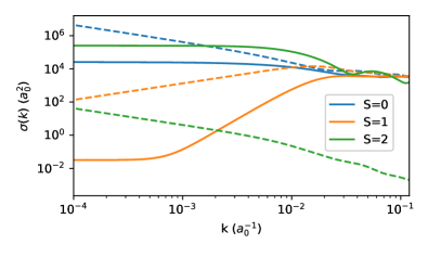
Figure 1: Momentum dependence of elastic cross sections (solid lines) given by (46) and ionization cross sections (dashed lines) given by (47) for the 4–4 system.

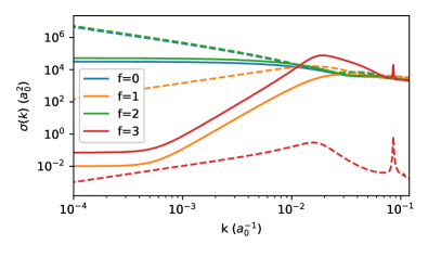
Figure 2: Cross sections for the 3–3 system, as in figure 1, with both ³He^∗ atoms in their lower hyperfine level. Note the sharp structures at around  $10^{-1}$ $a_{0}$ are a result of resonances in the potentials for scattering with $l=5$.

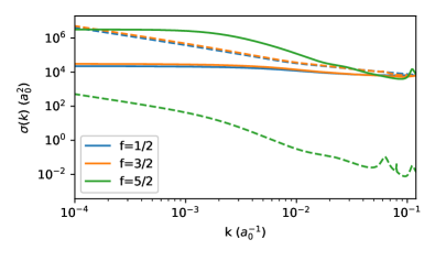
Figure 3: Cross sections for the 3–4 system, as in figure 2, with the ³He^∗ atom in its lower hyperfine level.

At low energies the $T$-matrix elements used in the calculation of the rates should have an energy dependence determined by the Wigner threshold behavior of the $T$-matrix elements for a $R^{-n}$ interaction, that is Mies2000

$$|T_{aa}|^{2}\underset{k_{a}\rightarrow 0}{\sim}\left\{\begin{array}[]{lll}\left[k_{a}^{2l+1}\right]^{2},&(2l+1)<(n-2),&n>3\\ \left[k_{a}^{n-2}\right]^{2},&(2l+1)>(n-2),&n>3\\ \left[k_{a}\ln k_{a}\right]^{2},&l=0,&n=3\\ k_{a}^{2},&l\geq 1,&n=3\end{array}\right.$$ (73)

and

$$|T_{a^{\prime}a}|^{2}\underset{k_{a}\rightarrow 0}{\sim}k_{a}^{2l+1},\quad a^{\prime}\neq a.$$ (74)

In all cases, a dependence of $k^{0}_{\Gamma}$ is observed as $k_{\Gamma}\rightarrow 0$ in the elastic cross sections, however this is a result of different processes. The behavior of the cross sections for the homonuclear systems is a consequence of the selection rules $(-1)^{l-S}=1$ for the 4–4 system and $(-1)^{l-f}=-1$ for the 3–3 system (with $f_{1}=f_{2}=\frac{3}{2}$), which require $l$ even (odd) for $S$ even (odd) for the 4–4 system and $l$ odd (even) for $f$ even (odd) for the 3–3 system. Since the matrix elements (34) of the spin-dipole $R^{-3}$ interaction vanish for $s$-wave elastic scattering but are non-zero for elastic $p$-wave scattering, the threshold behavior of the elastic cross sections is only determined by the $R^{-3}$ interaction when $s$-wave scattering is excluded (as is the case for the 4–4 system with $S=1$ and the 3–3 system with $f=0,2$), in which case the dependence is given by $k_{\Gamma}^{0}$. When $s$-wave scattering is present (the 4–4 system with $S=0,2$, the 3–3 system with $f=1,3$, and the 3–4 system where there is no selection rule) the threshold behavior is due to the long-range $R^{-6}$ interaction and the elastic cross sections have the variation $k_{\Gamma}^{0}$.

At higher energies where elastic $p$-wave scattering is due to the $R^{-6}$ interaction, the elastic cross sections have a $k_{\Gamma}^{4}$ dependence. As the inelastic (ionization) cross sections have the threshold behavior $k_{\Gamma}^{2l+1}$ Julienne1989 ; Mies2000 , the $s$-wave ionization cross sections vary as $k_{\Gamma}^{-1}$ at very low energies whereas the $p$-wave cross sections vary as $k_{\Gamma}^{1}$.

There are also several peaks observable near $k=0.1~{}a_{0}^{-1}$. We have identified these as resonances that occur in the $l=5$ partial wave for the ${}^{5}\Sigma_{g}$ and ${}^{3}\Sigma_{u}$ potentials. We note the selection rule in the 4–4 system suppresses this resonance in the $S=2$ case.

IV.2 Rates

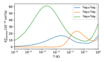
Figure 4: Thermally averaged spin-stretched elastic rates for the 3–3, 3–4 and 4–4 systems.

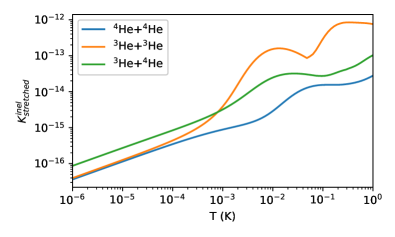
Figure 5: Thermally averaged spin-stretched inelastic rates for the 3–3, 3–4 and 4–4 systems.

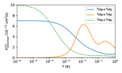
Figure 6: Thermally averaged spin-stretched ionization rates for the 3–3, 3–4 and 4–4 systems. The dashed line for the 3–4 rate indicates the rate is a factor of 10 larger than shown in the graph.

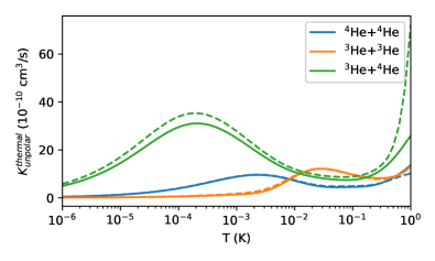
Figure 7: Thermally averaged total unpolarized thermalization rates for the 3–3, 3–4 and 4–4 systems. Solid lines correspond to the multichannel calculation and dashed lines to the single-channel calculation.

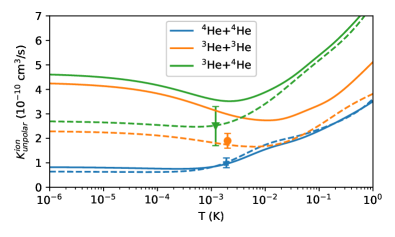
Figure 8: Thermally averaged total unpolarized ionization rates for the 3–3, 3–4 and 4–4 systems. Solid and dashed lines correspond to the multichannel and single-channel calculations respectively. Experimental data points are shown for the 4–4 (star, Stas2006 ), 3–3 (circle, Stas2006 ) and 3–4 (triangle, McNamara2007 ) systems. Note that these experimental data points were extrapolated from a mixed population of magnetic sublevels to the completely unpolarized mixture using an approximate theory. Our unpolarized rates should be viewed as an upper bound for any mixture of magnetic sublevels.

In Figures. 4–6 we report thermally averaged elastic, inelastic and ionization rates respectively for spin-stretched initial states, that is, $S=2$ for the 4–4 system, $f=3\,(S=2)$ for the 3–3 system, and $f=\frac{5}{2}\,(S=2)$ for the 3–4 system. It can be seen that the ionization rates are much smaller than the elastic rates. In addition, the inelastic rates, which indirectly contribute to ionization, are even smaller for low temperatures. At higher temperatures these inelastic rates are more important, representing the dominant pathway for ionization, although they remain smaller than the elastic rates. The relative magnitudes of these cross sections are the reason for long lifetimes of a spin-stretched gas of metastable helium.

The unpolarized thermal and ionization rates are shown in Fig. 7 and Fig. 8 respectively. As expected, the ionization rates for polarized systems in a spin-stretched initial state are strongly suppressed compared to those for unpolarized systems, the suppression being $O(10^{-4})$ for the 4–4 and 3–4 systems and $O(10^{-5})$ for the 3–3 system.

The single-channel calculations are shown in Fig. 7 and Fig. 8 as dashed lines. We can see reasonable agreement with the 4–4 system, in which there is little difference between the couplings included in the multichannel and single-channel formalism, but there are much larger disagreements for the 3–3 and 3–4 systems. We believe this originates in the effective diabatic connection between the outer and inner regions of the calculation, which will be discussed in more detail in section IV.3.

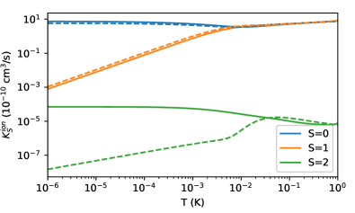
Figure 9: The multichannel and single-channel ionization rates for the 4–4 system shown as solid and dashed lines, respectively. Here $K^{\textrm{loss}}_{S}(T)=K(T;\Gamma,S,S\rightarrow\mathrm{PI})$. The disagreement for the $S=2$ channel is due to the perturbative treatment of the spin-dipole coupling.

We also show a comparison of unpolarized ionization rates for the 4–4 system between the single-channel and multichannel calculations in Fig. 9. We can see that the single-channel calculation performs well for the $S=0,1$ channels, but fails to capture the correct $T\rightarrow 0$ form of the $S=2$ channel. This is due to the perturbative treatment of the spin-dipole coupling, connecting the $S=2$ channel to the $S=0$. We believe the radial-dependence of the ionization process is not well captured in the perturbative treatment as the scattering wave functions in the $l=2$ states do not represent very well the short-range properties of the complex singlet potential.

Our values for rates with spin-stretched and unpolarized mixtures should place rough lower and upper bounds, respectively, on the rates for an arbitrary mixture of magnetic sublevels in an experimental configuration.

IV.3 Comparison with other calculations

The present calculations for the 4–4 system essentially reproduce the results of Venturi et al. Venturi2000 although there are some differences arising from our use of the Przybytek and Jeziorski Przy2005 ${}^{5}V_{\Sigma}(R)$ potential rather than the older Stärck and Meyer SM1994 potential used by Venturi2000 .

Our calculated total unpolarized ionization coefficients are higher than those calculated by Stas2006 ; McNamara2007 ; Dickinson2007 using a two-stage semiclassical model, the differences at $T=1$ mK, for example, being approximately 30% and 15% larger for 3–3 system and 3–4 system respectively. As the semiclassical models assume 100% ionization at small $R$ in the $S=0,1$ states, in contrast to the use of a complex optical potential, it has been argued Dickinson2007 that these semiclassical models should give upper bounds to the ionization coefficients. However, we note that the calculations of Stas2006 ; McNamara2007 ; Dickinson2007 answer the question “what proportion of incoming flux will pass through to the short-range in the singlet or triplet state” by assuming a diabatic connection between the outer basis, best described by $f_{1}$ and $f_{2}$, and the inner basis, best described by $S$ and $i$. This is effectively a two-stage or “single-pass” model as all flux in the $S=0,1$ states at short range is completely lost through ionization while all flux in the $S=2$ state is assumed to be reflected outwards and leave the scattering region. Our single-channel calculations, through the sum over $l$ in equations (69)–(72), effectively apply this same description of a diabatic connection from the outer to inner basis.

We argue that the question “what proportion of incoming flux can return as outgoing flux” should instead be considered. This requires a three-stage model with a second diabatic connection from the inner to outer basis, where some states (i.e. higher hyperfine levels) are energetically forbidden. In these channels, the outgoing flux would be reflected inwards, remaining trapped in the system for multiple ionization attempts. Hence, some of our multichannel values are larger than those predicted by the semiclassical models.

IV.4 Comparison with experimental measurements

The elastic collision rate for the spin-polarized 4–4 system at $T=1.0\pm 0.1$ mK has been measured Browaeys2001 to be $\alpha=5\times 10^{-9}$ cm³/s to within a factor of 3. This compares with our theoretical value of $\alpha=2K=1.76\times 10^{-9}$ cm³/s. This is just within the range of experiment, although we note that small variations to the short-range parts of the potential Venturi2000 ; Cocks2010 can affect this.

A comparison of our calculated loss rates with the various calculated and measured loss rate coefficients reported in the literature is given in Table 1.

Table 1: Thermally averaged total unpolarized ionization rates for the 3–3, 3–4 and 4–4 systems in units of $10^{-10}$ cm³/s. Results from our present calculations, using ionization widths $\Gamma_{\text{M}}(R)$ and $\Gamma_{\text{GMS}}(R)$, denoted $K^{\text{th}}_{\text{M}}$ and $K^{\text{th}}_{\text{GMS}}$ respectively, and single-channel calculations $K^{\text{th}}_{\text{SC}}$ are compared to experimental values $K^{\text{exp}}$ and calculated values using simple two-stage semiclassical models $K^{\text{th}}_{\text{2S}}$ KM1999 ; Stas2006 ; McNamara2007 ; Mastwijk1998 ; Tol1999 . Numbers in brackets denote one standard deviation experimental errors.

	Ref.	T(mK)	$K^{\text{exp}}$	$K^{\text{th}}_{\text{M}}$	$K^{\text{th}}_{\text{GMS}}$	$K^{\text{th}}_{\text{SC}}$	$K^{\text{th}}_{\text{2S}}$
4–4	Mastwijk1998	$1.0$	$2.7(1.2)$	$0.831$	$0.830$	$0.82$
	Tol1999	$1.0$	$1.3(0.2)$	$0.831$	$0.830$	$0.82$
	KM1999	$0.5$	$3.8(1.1)$	$0.769$	$0.792$	$0.70$	$2.2$
	Stas2006	$1.9(1)$	$1.0(2)$	$0.931$	$0.956$	$1.01$	$0.80$
3–3	KM1999	$0.5$	$11.0(4)$	$3.23$	$3.41$	$1.94$	$11$
	Stas2006	$2.0(3)$	$1.9(3)$	$2.90$	$2.98$	$1.74$	$1.8$
3–4	McNamara2007	$1.2(1)$	$2.9(8)$	$3.61$	$3.57$	$2.52$	$2.9$

The present loss rate coefficients are in good agreement with the measurements of Stas2006 for the 4–4 system, but our 3–4 and 3–3 results are above the measurements of McNamara2007 and Stas2006 . However, we note that these experiments were carried out in a MOT where the magnetic sublevel mixture was not an unpolarized set. These papers used the semiclassical theory discussed above to then rescale their experimental results to estimate an experimental unpolarized rate, however we believe this has underestimated the true value. Note that there are significant discrepancies between the experimental values, due possibly to approximations in the experimental analysis such as the neglect of the magnetic substate distribution Stas2006 . The large discrepancy with the 3–3 and 4–4 semiclassical calculations of KM1999 is not surprising as these calculations are based upon several incorrect assumptions that significantly overestimate the rate coefficients Stas2006 .

V Summary

Scattering and ionizing cross sections and rates have been calculated for ultracold collisions between metastable helium atoms using a fully quantum-mechanical close-coupled formalism. Homonuclear collisions of the bosonic ⁴He${}^{*}+{}^{4}$He^∗ and fermionic ³He${}^{*}+{}^{3}$He^∗ systems, and heteronuclear collisions of the mixed ³He${}^{*}+{}^{4}$He^∗ system, were investigated over a temperature range 1 $\mu$K to 1 K. Carefully constructed Born-Oppenheimer molecular potentials were used to describe the electrostatic interaction between the colliding atoms. The loss through ionization from the ${}^{1,3}\Sigma$ states was represented by complex optical potentials. Magnetic spin-dipole mediated transitions from the ${}^{5}\Sigma$ state were included and results obtained for spin-polarized and non spin-polarized systems.

The calculated scattering and ionization cross sections have the appropriate Wigner threshold behavior for momenta below $k\approx 10^{-3}\,a_{0}^{-1}$, and exhibit several peaks near $k=0.1\;a_{0}^{-1}$, identified as resonances in the $l=5$ partial wave.

Thermally averaged rates for spin-stretched initial states ($S=2$ for the 4–4 system, $f=3$ for the 3–3 system, and $f=\frac{5}{2}$ for the 3–4 system) are greatest for elastic scattering, $O(10^{-5})$ smaller for ionization, and range from $O(10^{-7})$ smaller at 1 $\mu$K to $O(10^{-5})$ smaller at 1 K for inelastic scattering. We note that there is a significantly larger ionization rate of the 3–4 system, which leads to stronger losses for dual-species mixtures. The thermally averaged rates for unpolarized systems are enhanced by $O(10^{4})$ for the 4–4 and 3–4 systems, and $O(10^{5})$ for the 3–3 system, compared to the spin-stretched rates.

The total unpolarized ionization rates are higher than those calculated using two-stage semiclassical models Stas2006 ; McNamara2007 based upon a diabatic connection between the basis states in the inner and outer regions. It has been argued Dickinson2007 that these semiclassical models should give upper bounds on ionization rates but we suggest that a three-stage semiclassical model which includes a second diabatic connection is more appropriate and that such a model would give higher rates.

Finally, a perturbed single channel model was developed in which hyperfine couplings and splittings are neglected but the effects of the different quantum statistical symmetries are included. It was found that this single-channel approximation follows a similar trend to the two-stage semi-classical model and underestimates the ionization rates for the 3–3 and 3–4 systems.

Appendix A Basis states and matrix elements

Matrix elements of $\hat{H}_{\text{el}}$ and $\hat{H}_{\text{sd}}$ in the $\{|a_{12}\rangle\}$ basis (21) are required whereas they are most easily evaluated in the $\{|\alpha\rangle\}$ basis (33). The first basis

$$|a_{12}\rangle=|(S_{1},i_{1},f_{1})_{A};(S_{2},i_{2},f_{2})_{B};f,l,J,M_{J}\rangle$$ (75)

involves the couplings

$$\hat{\mathbf{S}}_{1}+\hat{\mathbf{i}}_{1}=\hat{\mathbf{f}}_{1},\quad\hat{\mathbf{S}}_{2}+\hat{\mathbf{i}}_{2}=\hat{\mathbf{f}}_{2},\quad\hat{\mathbf{f}}_{1}+\hat{\mathbf{f}}_{2}=\hat{\mathbf{f}},$$ (76)

with associated states

$$|(S_{1},i_{1},f_{1})_{A};(S_{2},i_{2},f_{2})_{B};f,m_{f}\rangle,$$ (77)

whereas the second basis

$$|\alpha\rangle=|(S_{1})_{A},(S_{2})_{B};S,M_{S}\rangle|l,m_{l}\rangle$$ (78)

is associated with the couplings

$$\hat{\mathbf{S}}_{1}+\hat{\mathbf{S}}_{2}=\hat{\mathbf{S}},\quad\hat{\mathbf{i}}_{1}+\hat{\mathbf{i}}_{2}=\hat{\mathbf{i}},\quad\hat{\mathbf{S}}+\hat{\mathbf{i}}=\hat{\mathbf{f}}$$ (79)

and the states

$$|(S_{1},i_{1})_{A};(S_{2},i_{2})_{B};S,i;f,m_{f}\rangle=\sum_{M_{S},m_{i}}C^{Sif}_{M_{S},m_{i},m_{f}}|(S_{1})_{A},(S_{2})_{B};S,M_{S}\rangle|(i_{1})_{A},(i_{2})_{B};i,m_{i}\rangle.$$ (80)

The relationship between states in the two couplings (76) and (79) is Brink68

$$|(S_{1},i_{1},f_{1})_{A};(S_{2},i_{2},f_{2})_{A};f,m_{f}\rangle=\sum_{S,i}[Sif_{1}f_{2}]^{1/2}\left\{\begin{matrix}{S_{1}}&{\!\!\!S_{2}}&{\!\!\!S}\cr{i_{1}}&{\!\!\!i_{2}}&{\!\!\!i}\cr{f_{1}}&{\!\!\!f_{2}}&{\!\!\!f}\cr\end{matrix}\right\}|(S_{1},i_{1})_{A};(S_{2},i_{2})_{B};S,i;f,m_{f}\rangle.$$ (81)

Finally, the first basis requires the coupling $\hat{\mathbf{f}}+\hat{\mathbf{l}}=\hat{\mathbf{J}}$ to give

$$|(S_{1},i_{1},f_{1})_{A};(S_{2},i_{2},f_{2})_{B};f,l,J,M_{J}\rangle=\sum_{m_{f},m_{l}}C^{flJ}_{m_{f},m_{l},m_{J}}|(S_{1},i_{1},f_{1})_{A};(S_{2},i_{2},f_{2})_{B};f,m_{f}\rangle|l,m_{l}\rangle.$$ (82)

Hence

$$\langle a_{12}^{\prime}|\hat{H}_{\text{el}}|a_{12}\rangle = \delta_{i_{1}^{\prime},i_{1}}\delta_{i_{2}^{\prime},i_{2}}\delta_{l^{\prime},l}[f_{1}^{\prime}f_{2}^{\prime}f_{1}f_{2}]^{1/2}\;\sum_{S^{\prime},S,i}[S^{\prime}S]^{1/2}[i]$$ (83)

$$\times\sum_{m_{f}^{\prime},m_{f},m_{l}}C^{f^{\prime}lJ^{\prime}}_{m_{f}^{\prime},m_{l},m_{J}^{\prime}}C^{flJ}_{m_{f},m_{l},m_{J}}\sum_{M_{S}^{\prime},M_{S},m_{i}}C^{S^{\prime}if^{\prime}}_{M_{S}^{\prime},m_{i},m_{f}^{\prime}}C^{Sif}_{M_{S},m_{i},m_{f}}$$

$$\times\left\{\begin{matrix}{S_{1}}&{\!\!\!S_{2}}&{\!\!\!S}\cr{i_{1}}&{\!\!\!i_{2}}&{\!\!\!i}\cr{f_{1}^{\prime}}&{\!\!\!f_{2}^{\prime}}&{\!\!\!f^{\prime}}\cr\end{matrix}\right\}\left\{\begin{matrix}{S_{1}}&{\!\!\!S_{2}}&{\!\!\!S}\cr{i_{1}}&{\!\!\!i_{2}}&{\!\!\!i}\cr{f_{1}}&{\!\!\!f_{2}}&{\!\!\!f}\cr\end{matrix}\right\}\;\langle(S_{1}^{\prime})_{A},(S_{2}^{\prime})_{B},S^{\prime},M_{S}^{\prime}|\hat{H}_{\text{el}}|(S_{1})_{A},(S_{2})_{B};S,M_{S}\rangle.$$

Transforming the matrix element into body-fixed states using (II.2) and then using their eigenvalue equation (II.2) gives

$$\langle(S_{1}^{\prime})_{A},(S_{2}^{\prime})_{B},S^{\prime},M_{S}^{\prime}|\hat{H}_{\text{el}}|(S_{1})_{A},(S_{2})_{B};S,M_{S}\rangle=\delta_{S_{1}^{\prime},S_{1}}\delta_{S_{2}^{\prime},S_{2}}\delta_{S^{\prime},S}\sum_{\Omega_{S}}D^{S\,\dagger}_{M_{S}^{\prime},\Omega_{S}}(\phi,\theta,0)D^{S}_{\Omega_{S},M_{S}}(\phi,\theta,0)\,{}^{2S+1}V_{\Sigma}(R).$$ (84)

The unitarity of the rotation matrix gives $\delta_{M_{S}^{\prime},M_{S}}$, the summations over the Clebsch-Gordan coefficients $\delta_{f^{\prime},f}\,\delta_{J^{\prime},J}\,\delta_{M_{J}^{\prime},M_{J}}$, and (83) reduces to (II.2).

Similarly, the matrix element of $\hat{H}_{\text{sd}}$ is

$$\langle a_{12}^{\prime}|\hat{H}_{\text{sd}}|a_{12}\rangle = \delta_{i_{1}^{\prime},i_{1}}\delta_{i_{2}^{\prime},i_{2}}[f_{1}^{\prime}f_{2}^{\prime}f_{1}f_{2}]^{1/2}\;\sum_{S^{\prime},S,i}\sum_{\begin{subarray}{c}m_{l},m_{f}\\ m_{i},M_{S}\end{subarray}}\sum_{\begin{subarray}{c}m_{l}^{\prime},m_{f}^{\prime}\\ M_{S}^{\prime}\end{subarray}}[S^{\prime}S]^{1/2}[i]\,C^{f^{\prime}l^{\prime}J^{\prime}}_{m_{f}^{\prime},m_{l}^{\prime},m_{J}^{\prime}}C^{flJ}_{m_{f},m_{l},m_{J}}C^{S^{\prime}if^{\prime}}_{M_{S}^{\prime},m_{i},m_{f}^{\prime}}C^{Sif}_{M_{S},m_{i},m_{f}}$$ (85)

$$\times\left\{\begin{matrix}{S_{1}^{\prime}}&{\!\!\!S_{2}^{\prime}}&{\!\!\!S^{\prime}}\cr{i_{1}}&{\!\!\!i_{2}}&{\!\!\!i}\cr{f_{1}^{\prime}}&{\!\!\!f_{2}^{\prime}}&{\!\!\!f^{\prime}}\cr\end{matrix}\right\}\left\{\begin{matrix}{S_{1}}&{\!\!\!S_{2}}&{\!\!\!S}\cr{i_{1}}&{\!\!\!i_{2}}&{\!\!\!i}\cr{f_{1}}&{\!\!\!f_{2}}&{\!\!\!f}\cr\end{matrix}\right\}\langle l^{\prime},m_{l}^{\prime}|\langle(S_{1}^{\prime})_{A},(S_{2}^{\prime})_{B},S^{\prime},M_{S}^{\prime}|\hat{H}_{\text{sd}}|(S_{1})_{A},(S_{2})_{B};S,M_{S}\rangle|l,m_{l}\rangle.$$

After using (34) and (35) for the matrix elements of $\hat{H}_{\mathrm{sd}}$ in the $\{|\alpha\rangle\}$ basis, the summations over magnetic quantum numbers can be reduced to summations over the three independent quantities $M_{S}$, $\epsilon=M_{S}^{\prime}-M_{S}$ and $\tau=m_{l}-M_{J}$ since

$$M_{S}^{\prime}=M_{S}+\epsilon,\quad m_{f}=\tau,\quad m_{f}^{\prime}=\tau+\epsilon,\quad m_{l}=M_{J}-\tau,\quad m_{l}^{\prime}=M_{J}-\tau-\epsilon,\quad m_{i}=\tau-M_{S}.$$ (86)

These relationships give $M_{J}^{\prime}=m_{f}^{\prime}+m_{l}^{\prime}=m_{f}+m_{l}=M_{J}$. As only three Clebsch-Gordan coefficients now involve $M_{S}$, the summation over $M_{S}$ can be performed:

$$\sum_{M_{S}}C^{{\,2}{\,S}{\,S^{\prime}}}_{{\,\epsilon,}{\,M_{S},}{\,M_{S}+\epsilon}}C^{{\,S^{\prime}}{\,i_{1}}{\,f^{\prime}}}_{{\,M_{S}+\epsilon,}{\,\tau-M_{S},}{\,\tau+\epsilon}}C^{{\,S}{\,i_{1}}{\,f}}_{{\,M_{S},}{\,\tau-M_{S},}{\,\tau}}=(-1)^{-(f^{\prime}+i_{1}+S)}[S^{\prime}f]^{1/2}C^{{\,2}{\,f}{\,f^{\prime}}}_{{\,\epsilon,}{\,\tau,}{\,\epsilon+\tau}}\left\{\begin{matrix}{2}&{\!\!\!S}&{\!\!\!S^{\prime}}\cr{i_{1}}&{\!\!\!f^{\prime}}&{\!\!\!f}\cr\end{matrix}\right\}.$$ (87)

Similarly the summation over $\epsilon$ gives

$$\sum_{\epsilon}C^{{\,f}{\,2}{\,f^{\prime}}}_{{\,\tau,}{\,\epsilon,}{\,\epsilon+\tau}}C^{{\,f^{\prime}}{\,l^{\prime}}{\,J^{\prime}}}_{{\,\epsilon+\tau,}{\,M_{J}-\epsilon-\tau,}{\,M_{J}}}C^{{\,2}{\,l^{\prime}}{\,l}}_{{\,\epsilon,}{\,M_{J}-\epsilon-\tau,}{\,M_{J}-\tau}}=(-1)^{f+l^{\prime}+J^{\prime}}[f^{\prime}l]^{1/2}C^{{\,f}{\,l}{\,J^{\prime}}}_{{\,\tau,}{\,M_{J}-\tau,}{\,M_{J}}}\left\{\begin{matrix}{f}&{\!\!\!2}&{\!\!\!f^{\prime}}\cr{l^{\prime}}&{\!\!\!J^{\prime}}&{\!\!\!l}\cr\end{matrix}\right\}.$$ (88)

The remaining summation over $\tau$ gives $\delta_{J^{\prime},J}$ and the matrix element reduces to (39).

For the 3–3 and 4–4 systems, the matrix elements $\langle a^{\prime}|\hat{H}_{\mathrm{el}}|a\rangle$ and $\langle a^{\prime}|\hat{H}_{\mathrm{sd}}|a\rangle$ are symmetrized combinations of $\langle a_{x^{\prime}y^{\prime}}^{\prime}|\hat{H}_{\mathrm{el}}|a_{xy}\rangle$ and $\langle a_{x^{\prime}y^{\prime}}^{\prime}|\hat{H}_{\mathrm{sd}}|a_{xy}\rangle$ respectively, where $x$ and $y$ can take the values 1 or 2. These combinations give rise to a selection rule $(-1)^{l-S-i}=1$, and two factors $\sqrt{2-\delta_{f_{1}f_{2}}}$ and $\sqrt{2-\delta_{f_{1}^{\prime}f_{2}^{\prime}}}$. The matrix elements both have the form

$$\langle a^{\prime}|\hat{H}_{z}|a\rangle=\langle a_{12}^{\prime}|\hat{H}_{z}\hat{P}_{Si}\sqrt{(2-\delta_{f_{1}f_{2}})(2-\delta_{f_{1}^{\prime}f_{2}^{\prime}})}|a_{12}\rangle$$ (89)

where $\hat{H}_{z}=\hat{H}_{\mathrm{el}}$ or $\hat{H}_{\mathrm{sd}}$, and $\hat{P}_{Si}$ is defined by its action on the $\{S,i\}$ basis:

$$\hat{P}_{Si}|S_{1},S_{2},S,M_{S}\rangle|i_{1},i_{2},i,m_{i}\rangle|l,m_{l}\rangle=\frac{1+(-1)^{l-S-i}}{2}|S_{1},S_{2},S,M_{S}\rangle|i_{1},i_{2},i,m_{i}\rangle|l,m_{l}\rangle$$ (90)

Appendix B Integration of multichannel equations

The multichannel equations (10) have been solved using two methods to verify the numerical procedure using the Julia programming language Julia . The first method uses the renormalized Numerov method Johnson1978 on a linear grid of points consisting of connected regions within which a fixed step size is used. The second method uses a Runge-Kutta method with an adaptive step size to solve the equations (10) recast as first-order equations.

The solutions were found by integrating a linearly independent set of wave functions outwards from $R=1\,a_{0}$ to $R=100\,a_{0}$ with the inner boundary conditions $\mathbf{G}(R=1)=0$ and integrating a linearly independent set of wave functions inwards from $R=1000\,a_{0}$ to $R=100\;a_{0}$. The outer boundary conditions were specified that all closed channels should be zero at $R=1000\;a_{0}$. These two sets of solutions were matched to find a complete set of allowed solutions (the number of solutions is the same as the number of open channels) that satisfy both the inner and outer boundary conditions.

These solutions must then be matched to their asymptotic form (58) to determine the S matrix. As the spin-dipole term decays slowly as $R^{-3}$, this requires integration of the solutions (consisting only of open channels) to a point well beyond $R=1000\,a_{0}$. We found that this integration is prone to accumulated numerical error and so we chose to instead solve the integral equations Joachain1983 for the coefficients of the asymptotic matching of (58). In this manner, the solutions $\mathbf{G}(R)$ were expressed in the form

$$\mathbf{G}(R)=\mathbf{A}(R)\mathbf{J}_{l_{a}}(k_{a}R)+\mathbf{B}(R)\mathbf{N}_{l_{a}}(k_{a}R).$$ (91)

The matrices $\mathbf{A}(R)$ and $\mathbf{B}(R)$ satisfy the differential equations

$$\frac{d\mathbf{A}}{dR} = -\frac{1}{k_{a}}\mathbf{N}_{l_{a}}(k_{a}R)\mathcal{U}(R)\mathbf{G}(R),$$ (92)

$$\frac{d\mathbf{B}}{dR} = \frac{1}{k_{a}}\mathbf{J}_{l_{a}}(k_{a}R)\mathcal{U}(R)\mathbf{G}(R),$$ (93)

where

$$\mathcal{U}_{a^{\prime}a}(R)=\frac{2\mu}{\hbar^{2}}[V_{a^{\prime}a}(R)-V_{aa}(R\rightarrow\infty)\delta_{a^{\prime},a}],$$ (94)

and vary much more smoothly than the wave functions $\mathbf{G}(R)$.

References

- (1) I. Bloch, J. Dalibard and W. Zwerger, Many-body physics with ultracold gases, Rev. Mod. Phys. 80, 885 (2008).
- (2) M. Tsubota, M. Kobayashi and H. Takeuchi, Quantum hydrodynamics, Phys. Rep. 522, 191 (2013).
- (3) N. R. Cooper, J. Dalibard and I. B. Spielman, Topological bands for ultracold atoms, Rev. Mod. Phys. 91, 015005 (2019).
- (4) W. Vassen, C. Cohen-Tannoudji, M. Leduc, D. Boiron, C. I. Westbrook, A. Truscott, K. Baldwin, G. Birkl, C. Cancio, and M. Trippenbach, Cold and trapped metastable noble gases, Rev. Mod. Phys. 84, 175 (2012)
- (5) R. J.Stas, J. M. McNamara, W. Hogervorst, and W. Vassen, Simultaneous magneto-optical trapping of a boson-fermion mixture of metastable helium atoms, Phys. Rev. Lett. 93, 053001 (2004)
- (6) T. Jeltes, J. M. McNamara, W. Hogervorst, W. Vassen, V. Krachmalnicoff, M. Schellekens, A. Perrin, H. Chang, D. Boiron, A. Aspect and C. I. Westbrook Comparison of the Hanbury-Brown-Twiss effect for bosons and fermions, Nature 445, 402 (2007).
- (7) R. Khakimov, B. Henson, D. Shin, S. Hodgman, R. Dall, K. Baldwin and A. Truscott, Ghost imaging with atoms, Nature 540, 100 (2016).
- (8) B. M. Henson, R. I. Khakimov, R. G. Dall, K. G. H. Baldwin, L.-Y. Tang and A. G. Truscott Precision Measurement for Metastable Helium Atoms of the 413 nm Tune-Out Wavelength at Which the Atomic Polarizability Vanishes Phys. Rev. Lett. 115, 043004 (2015).
- (9) V. Venturi and I. B. Whittingham, Close-coupled calculation of field-free collisions of cold metastable helium atoms, Phys. Rev. A 61, 060703(R) (2000)
- (10) O. Sirjean, S. Seidelin, J. Vianna Gomes, D. Boiron, C. I. Westbrook, A. Aspect, and G. V. Shlyapnikov, Ionization rates in a Bose-Einstein condensate of metastable helium, Phys. Rev. Lett. 89, 220406 (2002)
- (11) H. C. Mastwijk, J. W. Thomsen, P. van der Straten, and A. Niehaus, Optical collisions of cold metastable helium atoms, Phys. Rev. Lett. 80, 5516 (1998)
- (12) P. J. J. Tol, N. Herschbach, E. A. Hessels, W. Hogervorst, and W. Vassen, Large numbers of cold metastable helium atoms in a magneto-optical trap, Phys. Rev. A 60, R761 (1999)
- (13) M. Kumakura and N. Morita, Laser trapping of metastable 3He atoms: Isotopic difference in cold Penning collisions, Phys. Rev. Lett. 82, 2848 (1999)
- (14) R. J. W. Stas, J. M. McNamara, W. Hogervorst, and W. Vassen, Homonuclear ionizing collisions of laser-cooled metastable helium atoms, Phys. Rev. A 73, 032713 (2006)
- (15) P. L. Leo, V. Venturi, I. B. Whittingham, and J. F.Babb, Ultracold collisions of metastable helium atoms, Phys. Rev. A 64, 042710 (2001)
- (16) J. M. McNamara, R. J. W. Stas, W. Hogervorst, and W. Vassen, Heteronuclear ionizing collisions between laser-cooled metastable helium atoms, Phys. Rev. A 75, 062715 (2007)
- (17) A. S. Dickinson, Quantum reflection model for ionization rate coefficients in cold metastable helium collisions, J. Phys. B: At. Mol. Opt. Phys 40, F237 (2007)
- (18) P. S. Julienne and F. H. Mies, Collisions of ultracold trapped atoms, J. Opt. Soc. Am. B 6, 2257 (1989)
- (19) D. G. Cocks, G. Peach, and I. B. Whittingham, Long-range states in excited ultracold 3HeHe∗ dimers, J. Phys. B: At. Mol. Opt. Phys 48, 115205 (2015)
- (20) S. D. Rosner and F. M. Pipkin, Hyperfine structure of the 2 3S1 state of He3, Phys. Rev. A 1, 571 (1970)
- (21) T. J. Beams, G. Peach, and I. B. Whittingham, Spin-dipole-induced lifetime of the least-bound state of HeHe, Phys. Rev. A 74, 014702 (2006)
- (22) P. S. Julienne, Ultracold collisions of Atoms and Molecules, in Scattering: Scattering and Inverse Scattering in Pure and Applied Science, editors P. Sabatier and E. R. Pike (Academic Press, London, 2002), p. 1081
- (23) B. J. Garrison, W. H. Miller, and H. F. Schaffer, Penning and associative ionization of triplet metastable helium atoms, J. Chem. Phys. 59, 3193 (1973)
- (24) F. H. Mies, A scattering theory of diatomic molecules: General formalism using the channel state representation, Mol. Phys. 41, 953 (1980)
- (25) G. Peach, D. G. Cocks, and I. B. Whittingham, Ultracold collisions in metastable helium, J. Phys: Conf. Series 810, 012003 (2017)
- (26) M. J. Seaton, Quantum defect theory I. General formulation, Proc. Phys. Soc. 88, 801 (1966)
- (27) M. J. Seaton, Strong coupling in optically allowed atomic transitions produced by electron impact, Proc. Phys. Soc. 77, 174 (1961)
- (28) S. Geltman, Topics in Atomic Collision Theory (Academic, New York, 1969), p. 183
- (29) M. Przybytek and B. Jeziorski, Bounds for the scattering length of spin-polarized helium from high-accuracy electronic structure calculations, J. Chem. Phys. 123, 134315 (2005)
- (30) M. W. Müller, A. Merz, M.-W. Ruf, H. Hotop, W. Meyer, and M. Movre, Experimental and theoretical studies of the Bi-excited collision systems He)+ He at thermal and subthermal kinetic energies, Z. Phys. D: At. Mol. Clusters 21, 89 (1991)
- (31) F. H. Mies and M. Raoult, Analysis of threshold effects in ultracold atomic collisions, Phys. Rev. A 62, 012708 (2000)
- (32) J. Stärck and W. Meyer, Long-range interaction potential of the state of He2, Chem. Phys. Lett. 225, 229 (1994)
- (33) A. Browaeys, A. Robert, O. Sirjean, J. Poupard, S. Nowak, D. Boiron, C. I. Westbrook, and A. Aspect, Thermalization of magnetically trapped metastable helium, Phys. Rev. A 64, 034703 (2001)
- (34) D. M. Brink and G. R. Satchler, Angular Momentum, 2nd ed. (Clarendon Press, Oxford, 1968)
- (35) J. Bezanson, A. Edelman, S. Karpinski, and V. B. Shah, Julia: A fresh approach to numerical computing, Siam Rev. 59, 65 (2017)
- (36) B. R. Johnson, The renormalized Numerov method applied to calculating bound states of the coupled-channel Schroedinger equation, J. Chem. Phys. 69, 4678 (1978)
- (37) D. G. Cocks, I. B. Whittingham and G. Peach, Effects of non-adiabatic and Coriolis couplings on the bound states of He(23S)+He(23P) J. Phys. B: At. Mol. Opt. Phys. 43, 135102 (2010).
- (38) C. J. Joachain, Quantum Collision Theory, third edition, (North Holland, Amsterdam, 1983).