Combinatorial reciprocity for the chromatic polynomial and the chromatic symmetric function

Abstract.

Let $G$ be a graph, and let $\chi_{G}$ be its chromatic polynomial. For any non-negative integers $i,j$, we give an interpretation for the evaluation $\chi_{G}^{(i)}(-j)$ in terms of acyclic orientations. This recovers the classical interpretations due to Stanley and to Greene and Zaslavsky respectively in the cases $i=0$ and $j=0$. We also give symmetric function refinements of our interpretations, and some extensions. The proofs use heap theory in the spirit of a 1999 paper of Gessel.

1. Introduction

Let $G$ be a (finite, undirected) graph. A $q$-coloring of $G$ is an attribution of a color in $\{1,2,\ldots,q\}$ to each vertex of $G$. A $q$-coloring is called proper if any pair of adjacent vertices get different colors. The chromatic polynomial of $G$ is the polynomial $\chi_{G}$ such that for all positive integers $q$, the evaluation $\chi_{G}(q)$ is the number of proper $q$-colorings.

In this article we provide a combinatorial interpretation for the evaluations of the polynomial $\chi_{G}(q)$ and of its derivatives $\chi_{G}^{(i)}(q)$ at negative integers. Let us state this result. Recall that an orientation of $G$ is called acyclic if it does not have any directed cycle. A source of an orientation is a vertex without any ingoing edge. For a set $U$ of vertices of $G$, we denote $G[U]$ the subgraph of $G$ induced by $U$, that is, the graph having vertex set $U$ and edge set made of the edges of $G$ with both endpoints in $U$. The following is our main result about $\chi_{G}$, where we use the notation $[n]:=\{1,\ldots,n\}$ for a positive integer $n$, and the convention $[0]=\emptyset$.

Theorem 1.1.

Let $G$ be a graph with vertex set $[n]$. For any non-negative integers $i,j$, $(-1)^{n-i}\chi_{G}^{(i)}(-j)$ counts the number of tuples $((V_{1},\gamma_{1}),\ldots,(V_{i+j},\gamma_{i+j}))$ such that

• $V_{1},\ldots,V_{i+j}$ are disjoint subsets of vertices, such that $\bigcup_{k}V_{k}=[n]$,

• for all $k\in[i+j]$, $\gamma_{k}$ is an acyclic orientation of $G[V_{k}]$,

• for $k\in[i]$, $V_{k}\neq\emptyset$ and $\gamma_{k}$ has a unique source which is the vertex $\min(V_{k})$.

We will also prove a generalization of Theorem 1.1 (see Theorem 4.5), and a refinement at the level of the chromatic symmetric function (see Theorem 5.6). As we explain in Section 4, the cases $i=0$ and $j=0$ of Theorem 1.1 are classical results due to Stanley [10] and to Greene and Zaslavsky [7] respectively. However these special cases are usually presented in terms of colorings (instead of partitions of the vertex set) and global acyclic orientations (instead of suborientations). A version of Theorem 1.1 in this spirit is given in Corollary 4.4.

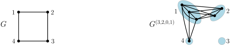
Figure 1. Left: A graph $G$ on 4 vertices, having chromatic polynomial $\chi_{G}(q)=q^{4}-4q^{3}+6q^{2}-3q$. Right: The graph $G^{(3,2,0,1)}$.

Let us illustrate Theorem 1.1 for the graph $G$ represented in Figure 1. For $i=j=1$, one needs to counts the pairs $((V_{1},\gamma_{1}),(V_{2},\gamma_{2}))$, where $V_{1}\uplus V_{2}=\{1,2,3,4\}$, $\gamma_{1}$ is an acyclic orientations of $G[V_{1}]$ with unique source $\min(V_{1})$, and $\gamma_{2}$ is any acyclic orientation of $G[V_{2}]$. The number of valid pairs with $V_{1}$ of size 1 (resp. 2, 3, 4) is 16 (resp. 8, 4, 3). This gives a total of 31 pairs which, as predicted by Theorem 1.1, is equal to $-\chi_{G}^{\prime}(-1)$.

In many ways, it feels like Theorem 1.1 should have been discovered earlier. Our proof is based on the theory of heaps, which takes its root in the work of Cartier and Foata [1], and has been popularized by Viennot [13]. In fact, our proof is in the same spirit as the one used by Gessel in [6], and subsequently by Lass in [9] (see also the recent preprint [3]). It consists in showing that well-known counting lemmas for heaps imply a relation between proper colorings and acyclic orientations. We recall the basic theory of heaps and their enumeration in Section 2. Theorem 1.1 is proved in Section 3. In Section 4, we discuss some reformulations, and extensions of Theorem 1.1 and their relations to the results in [6, 7, 9, 10]. In Section 5, we lift Theorem 1.1 at the level of the chromatic symmetric function.

2. Heaps: definition and counting lemmas

In this section we recall the basic theory of heaps. We fix a graph $G=([n],E)$ throughout.

2.1. Heaps of pieces

We first define $G$-heaps. Our (slightly unconventional) definition is in terms of acyclic orientations of a graph related to $G$. Let $\mathbb{N}=\{0,1,2,\ldots\}$ be the set of non-negative integers. For a tuple $\mathbf{m}=(m_{1},\cdots,m_{n})\in\mathbb{N}^{n}$, we define a graph $G^{\mathbf{m}}:=(V^{\mathbf{m}},E^{\mathbf{m}})$ with vertex set

$$V^{\mathbf{m}}:=\{v_{i}^{k}\}_{i\in[n],~{}k\in[m_{i}]},$$

and edge set defined as follows:

• for every vertex $i\in[n]$ of $G$ there is an edge of $G^{\mathbf{m}}$ between $v_{i}^{k}$ and $v_{i}^{\ell}$ for all $k,\ell\in[m_{i}]$,

• for every pair of adjacent vertices $i,j\in[n]$ of $G$ there is an edge of $G^{\mathbf{m}}$ between $v_{i}^{k}$ and $v_{j}^{\ell}$ for all $k\in[m_{i}]$ and all $\ell\in[m_{j}]$.

The notation $G^{\mathbf{m}}$ is illustrated in Figure 1 (right).

Definition 2.1.

A $G$-heap of type $\mathbf{m}$ is an acyclic orientation of the graph $G^{\mathbf{m}}$ such that for all $i\in[n]$ and for all $1\leq k<\ell\leq m_{i}$ the edge between $v_{i}^{k}$ and $v_{i}^{\ell}$ is oriented toward $v_{i}^{\ell}$. The vertices $v_{i}^{k}$ of $G^{\mathbf{m}}$ are called pieces of type $i$ of the $G$-heap.

Remark 2.2.

A more traditional definition of heaps is in terms of partially ordered sets. Namely, a $G$-heap of type $\mathbf{m}$ is commonly defined as a partial order $\prec$ on the set $V^{\mathbf{m}}$ such that

1. for any vertex $i\in[n]$, $v_{i}^{1}\prec v_{i}^{2}\prec\ldots\prec v_{i}^{m_{i}}$ ,

2. for any adjacent vertices $i,j\in[n]$, the set $\{v_{i}^{k}\}_{k\in{[m_{i}]}}\cup\{v_{j}^{\ell}\}_{\ell\in{[m_{j}]}}$ is totally ordered by $\prec$,

3. and the order relation is the transitive closure of the relations of type (a) and (b).

It is clear that this traditional definition is equivalent to Definition 2.1: the relation $\prec$ between vertices in $V^{\mathbf{m}}$ simply encodes the existence of a directed path between these vertices. In fact, Definition 2.1 already appears in [13, Definition (c), p.545].

Heaps were originally introduced to represent elements in a partially commutative monoid [1]. We refer the interested reader to [8, 13] for more information about heaps.

Recall that for an oriented graph, a vertex without ingoing edges is called a source, and a vertex without outgoing edges is called a sink. A piece of a heap $\mathbf{h}$ is called minimal (resp. maximal) if it is a source (resp. sink) in the acyclic orientation $\mathbf{h}$ of $G^{\mathbf{m}}$. A heap is called trivial if every piece is both minimal and maximal (which occurs when $G^{\mathbf{m}}$ consists of isolated vertices). A heap is a pyramid if it has a unique minimal piece.

Next, we define the generating functions of heaps, trivial heaps and pyramids. Let $\mathbf{x}=(x_{1},\ldots,x_{n})$ be commutative variables. Let $\mathcal{H}$, $\mathcal{T}$, and $\mathcal{P}$ be the set of heaps, trivial heaps, and pyramids respectively. We define

(1) $$H(\mathbf{x})=\sum_{\mathbf{h}\in\mathcal{H}}\mathbf{x}^{\mathbf{h}},~{}~{}~{}~{}T(\mathbf{x})=\sum_{\mathbf{h}\in\mathcal{T}}\mathbf{x}^{\mathbf{h}},~{}\textrm{ and }~{}~{}~{}P(\mathbf{x})=\sum_{\mathbf{h}\in\mathcal{P}}\frac{\mathbf{x}^{\mathbf{h}}}{{|\mathbf{h}|}},$$

where ${|\mathbf{h}|}$ is the number of pieces in the heap $\mathbf{h}$, and $\displaystyle\mathbf{x}^{\mathbf{h}}:=\prod_{i=1}^{n}x_{i}^{\#\textrm{ pieces of type }i\textrm{ in }\mathbf{h}}$. In other words, these generating functions, which are formal power series in $x_{1},\ldots,x_{n}$, count heaps according to the number of pieces of each type.

Example 2.3.

For the graph $G$ represented in Figure 1, the generating functions $T$, $H$, $P$ have the following expansions:

$$T(\mathbf{x}) = 1+x_{1}+x_{2}+x_{3}+x_{4}+x_{1}x_{3}+x_{2}x_{4}.$$

$$H(\mathbf{x}) = 1+x_{1}+x_{2}+x_{3}+x_{4}$$

$$+x_{1}^{2}+x_{2}^{2}+x_{3}^{2}+x_{4}^{2}+x_{1}x_{3}+x_{2}x_{4}+2x_{1}x_{2}+2x_{2}x_{3}+2x_{3}x_{4}+2x_{4}x_{1}+\cdots$$

$$P(\mathbf{x}) = x_{1}+x_{2}+x_{3}+x_{4}$$

$$+\frac{1}{2}\left(x_{1}^{2}+x_{2}^{2}+x_{3}^{2}+x_{4}^{2}+2x_{1}x_{2}+2x_{2}x_{3}+2x_{3}x_{4}+2x_{4}x_{1}\right)+\cdots$$

2.2. Enumeration of heaps

We now state the classical relation between $H(\mathbf{x})$, $T(\mathbf{x})$, and $P(\mathbf{x})$. For a scalar $r$, we use the notation $r\mathbf{x}:=(r\,x_{1},\ldots,r\,x_{n})$.

Theorem 2.4 ([13]).

The generating functions of heaps, trivial heaps and pyramids are related by

(2) $$H(\mathbf{x})=\frac{1}{T(-\mathbf{x})},$$

and

(3) $$P(\mathbf{x})=-\ln(T(-\mathbf{x})).$$

Equations (2-3) are identities for formal power series in $x_{1},\ldots,x_{n}$. Observing that $T(\mathbf{x})$ has constant term 1 (corresponding to the empty heap), the right-hand side of (2) should be understood as $\sum_{n=0}^{\infty}(1-T(-\mathbf{x}))^{n}$ and the right-hand side of (3) should be understood as $\sum_{n=1}^{\infty}(1-T(-\mathbf{x}))^{n}/n$.

Theorem 2.4 will be proved using the following classical result.

Lemma 2.5 ([13]).

Let $S\subseteq[n]$. Let $\mathcal{H}_{S}$ be the set of $G$-heaps such that every minimal piece has type in $S$, and let $\mathcal{T}_{\overline{S}}$ be the set of trivial $G$-heaps such that every piece has type in $[n]\setminus S$. Then the generating functions

$$H_{S}(\mathbf{x})=\sum_{\mathbf{h}\in\mathcal{H}_{S}}\mathbf{x}^{\mathbf{h}},~{}\textrm{ and }~{}T_{\overline{S}}(\mathbf{x})=\sum_{\mathbf{h}\in\mathcal{T}_{\overline{S}}}\mathbf{x}^{\mathbf{h}},$$

are related by

(4) $$H_{S}(\mathbf{x})=\frac{T_{\overline{S}}(-\mathbf{x})}{T(-\mathbf{x})}.$$

Let us give a sketch of the standard proofs of Lemma 2.5 and Theorem 2.4. Observe first that the identity (4) is equivalent to

(5) $$\sum_{(\mathbf{h}_{1},\mathbf{h}_{2})\in\mathcal{H}_{S}\times\mathcal{T}}(-1)^{|\mathbf{h}_{2}|}\mathbf{x}^{\mathbf{h}_{1}}\mathbf{x}^{\mathbf{h}_{2}}=\sum_{\mathbf{h}\in\mathcal{T}_{\overline{S}}}(-1)^{|\mathbf{h}|}\mathbf{x}^{\mathbf{h}}.$$

We now explain how to prove (5) using a sign-reversing involution on $\mathcal{H}_{S}\times\mathcal{T}$. Given $\mathbf{h}_{1}\in\mathcal{H}_{S}$ of type $\mathbf{m}_{1}$ and $\mathbf{h}_{2}\in\mathcal{T}$ of type $\mathbf{m}_{2}$, we define $\mathbf{h}:=\mathbf{h}_{1}*\mathbf{h}_{2}$ as the heap of type $\mathbf{m}=\mathbf{m}_{1}+\mathbf{m}_{2}$ obtained from $\mathbf{h}_{1}$ by adding the pieces of $\mathbf{h}_{2}$ as new sinks. More precisely, $\mathbf{h}$ is the orientation of $G^{\mathbf{m}}$ such that the restriction to $G^{\mathbf{m}_{1}}$ is $\mathbf{h}_{1}$ and the vertices in $V^{\mathbf{m}}\setminus V^{\mathbf{m}_{1}}$ are sinks. Now, we fix a heap $\mathbf{h}$, and look at the set $\mathcal{S}_{\mathbf{h}}$ of pairs $(\mathbf{h}_{1},\mathbf{h}_{2})\in\mathcal{H}_{S}\times\mathcal{T}$ such that $\mathbf{h}_{1}*\mathbf{h}_{2}=\mathbf{h}$. If $\mathbf{h}\not\in\mathcal{T}_{\overline{S}}$, one can define a simple sign reversing involution on $\mathcal{S}_{\mathbf{h}}$ in order to prove that the contributions of the pairs $(\mathbf{h}_{1},\mathbf{h}_{2})\in\mathcal{S}_{\mathbf{h}}$ to (5) cancel out. This involution simply transfers a canonically-chosen piece of $\mathbf{h}$ between $\mathbf{h}_{1}$ and $\mathbf{h}_{2}$ (one can transfer any maximal piece of $\mathbf{h}$ which either has type in $S$ or is not minimal, so a canonical choice is to transfer the piece of minimal type among those). If $\mathbf{h}\in\mathcal{T}_{\overline{S}}$, then $\mathcal{S}_{\mathbf{h}}=\{(\epsilon,\mathbf{h})\}$, where $\epsilon$ is the empty heap, hence the contribution of $\mathcal{S}_{\mathbf{h}}$ to (5) is 1. This proves Lemma 2.5.

To prove Theorem 2.4, observe first that (2) is the special case $S=[n]$ of (4). It remains to prove (3). Let $t$ be an indeterminate. By differentiating the series $P(t\,\mathbf{x})$ (formally) with respect to $t$ we get

$$t\cdot\frac{\partial}{\partial t}P(t\,\mathbf{x})=t\cdot\frac{\partial}{\partial t}\sum_{\mathbf{h}\in\mathcal{P}}\frac{t^{|\mathbf{h}|}}{{|\mathbf{h}|}}\mathbf{x}^{\mathbf{h}}=\sum_{\mathbf{h}\in\mathcal{P}}t^{|\mathbf{h}|}\mathbf{x}^{\mathbf{h}}.$$

We now use the partition $\mathcal{P}=\biguplus_{k\in[N]}(\mathcal{H}_{\{k\}}\setminus\{\epsilon\})$, where $\epsilon$ is the empty heap. This, together with (4) gives

$$t\cdot\frac{\partial}{\partial t}P(t\,\mathbf{x})=\sum_{k=1}^{n}\left(H_{\{k\}}(t\,\mathbf{x})-1\right)=\sum_{k=1}^{n}\frac{T_{\overline{\{k\}}}(-t\,\mathbf{x})-T(-t\,\mathbf{x})}{T(-t\,\mathbf{x})}=\frac{-1}{T(-t\mathbf{x})}\sum_{k=1}^{n}T_{k}(-t\,\mathbf{x}),$$

where

$$T_{k}(\mathbf{x})=\sum_{\begin{subarray}{c}\mathbf{h}\in\mathcal{T}\\ \textrm{containing a piece of type }k\end{subarray}}\mathbf{x}^{\mathbf{h}}.$$

Finally, we observe that $\displaystyle\sum_{k=1}^{n}T_{k}(\mathbf{x})=\sum_{\mathbf{h}\in\mathcal{T}}{|\mathbf{h}|}\mathbf{x}^{\mathbf{h}}$. This gives

$$\frac{\partial}{\partial t}P(t\,\mathbf{x})=\frac{1}{T(-t\mathbf{x})}\cdot\sum_{\mathbf{h}\in\mathcal{T}}{|\mathbf{h}|}(-t)^{{|\mathbf{h}|}-1}\mathbf{x}^{\mathbf{h}}=\frac{-1}{T(-t\mathbf{x})}\cdot\frac{\partial}{\partial t}T(-t\,\mathbf{x}),$$

which, upon integrating (formally) with respect to $t$, gives (3).

3. Heaps, colorings, and orientations: proof of Theorem 1.1

This section is dedicated to the proof of Theorem 1.1. We fix a graph $G=([n],E)$ throughout.

Notation 3.1.

We denote by $R[[\mathbf{x}]]$ the ring of power series in $x_{1},\ldots,x_{n}$ with coefficients in a ring $R$. For a tuple $\mathbf{m}=(m_{1},\ldots,m_{n})\in\mathbb{N}^{n}$, we denote $\mathbf{x}^{\mathbf{m}}=x_{1}^{m_{1}}\cdots x_{n}^{m_{n}}$. For a power series $F(\mathbf{x})\in R[[\mathbf{x}]]$, we denote by $[\mathbf{x}^{\mathbf{m}}]F(\mathbf{x})$ the coefficient of $\mathbf{x}^{\mathbf{m}}$ in $F(\mathbf{x})$.

The first step is to express the chromatic polynomial of $G$ in terms of trivial heaps.

Lemma 3.2.

Let $T(\mathbf{x})$ be the generating function of trivial $G$-heaps defined in (1), and let $q$ be an indeterminate. Then,

(6) $$\chi_{G}(q)=[x_{1}\cdots x_{n}]T(\mathbf{x})^{q}.$$

The right-hand side in (6) has to be understood as the coefficient of $x_{1}\cdots x_{n}$ in the series $\displaystyle\exp(q\ln(T(\mathbf{x})):=\sum_{k=0}^{\infty}\frac{(q\ln(T(\mathbf{x})))^{k}}{k!}\in\mathbb{Q}[q][[\mathbf{x}]]$.

Proof.

Recall that a set of vertices $V\subseteq[n]$ is called independent if the vertices in $V$ are pairwise non-adjacent. There is an obvious equivalence between independent sets and trivial heaps, hence $T(\mathbf{x})$ can be thought as the generating function of independent sets.

Let $q$ be a positive integer. Observe that for any proper $q$-coloring, the set of vertices of color $i\in[q]$ is an independent set. In fact, upon denoting $V_{i}$ the set of vertices of color $i$, it is clear that a proper $q$-coloring can equivalently be seen as a $q$-tuple $(V_{1},\ldots,V_{q})$ of independent sets of vertices, which are disjoint and such that $\bigcup_{k\in[q]}V_{k}=[n]$. This immediately implies that (6) holds for the positive integer $q$. Since both sides of (6) are polynomials in $q$, the identity holds for an indeterminate $q$. ∎

Upon differentiating (6) $i$ times one gets

$$\chi_{G}^{(i)}(q)=\frac{\partial^{i}}{\partial q^{i}}[x_{1}\cdots x_{n}]T(\mathbf{x})^{q}=[x_{1}\cdots x_{n}]\frac{\partial^{i}}{\partial q^{i}}\exp\left(q\ln(T(\mathbf{x}))\right)=[x_{1}\cdots x_{n}]\ln(T(\mathbf{x}))^{i}T(\mathbf{x})^{q}.$$

In the right-hand side of the above equation, we are are extracting a coefficient of degree $n$, hence this expression is invariant under changing $\mathbf{x}$ into $-\mathbf{x}$ and multiplying by $(-1)^{n}$. Hence $(-1)^{n}\chi_{G}^{(i)}(q)=[x_{1}\cdots x_{n}]\ln(T(-\mathbf{x}))^{i}\,T(-\mathbf{x})^{q}$, and for a non-negative integer $j$,

(7) $$(-1)^{n-i}\chi_{G}^{(i)}(-j) = [x_{1}\cdots x_{n}](-\ln(T(-\mathbf{x})))^{i}(T(-\mathbf{x}))^{-j}$$

$$= [x_{1}\cdots x_{n}]P(\mathbf{x})^{i}H(\mathbf{x})^{j},$$

where the last equality follows from Theorem 2.4.

The next step is to relate heaps and pyramids to acyclic orientations. For a set $V\subseteq[n]$, let $\mathbf{x}^{V}$ be the monomial $x_{1}^{\delta_{1}}\cdots x_{n}^{\delta_{n}}$, where $\delta_{i}=1$ if $i\in V$ and $\delta_{i}=0$ otherwise.

Lemma 3.3.

Let $V\subseteq[n]$. The generating function $H(\mathbf{x})$ and $P(\mathbf{x})$ defined in (1) satisfy

(8) $$[\mathbf{x}^{V}]H(\mathbf{x}) =\#\textrm{ acyclic orientations of }G[V],$$

(9) $$[\mathbf{x}^{V}]P(\mathbf{x}) =\#\textrm{ acyclic orientations of }G[V]\textrm{ with unique source }\min(V),$$

where the right-hand side of (9) is interpreted as 0 if $V=\emptyset$.

Proof.

Let $\mathbf{m}=(\delta_{1},\ldots,\delta_{n})$, where $\delta_{i}=1$ if $i\in V$, and $\delta_{i}=0$ otherwise. Observe that $G[V]$ is isomorphic to the graph $G^{\mathbf{m}}$. By definition of $H$, the coefficient $[\mathbf{x}^{V}]H(\mathbf{x})$ counts the $G$-heaps of type $\mathbf{m}$, or equivalently the acyclic orientations of $G[V]$. This proves (8). Let us now assume $V\neq\emptyset$. By definition of $P$, one gets $[\mathbf{x}^{V}]P(\mathbf{x})=\frac{B}{|V|}$, where $B$ is the number pyramids of type $\mathbf{m}$, or equivalently the number of acyclic orientations of $G[V]$ with a single source. For $i\in V$, let $\mathcal{B}_{i}$ be the set of acyclic orientations of $G[V]$ with unique source $i$. It is not hard to see that $|\mathcal{B}_{i}|=|\mathcal{B}_{j}|$ for all $i,j\in V$. Indeed, a bijection between $\mathcal{B}_{i}$ and $\mathcal{B}_{j}$ can be constructed as follows: given $\gamma\in\mathcal{B}_{i}$, reverse all the edges of $\gamma$ on any directed path from $i$ to $j$. This proves (9). ∎

We now complete the proof of Theorem 1.1. For any non-negative integers $i,j$, (7) gives

(10) $$(-1)^{n-i}\chi_{G}^{(i)}(-j) = \sum_{V_{1}\uplus\cdots\uplus V_{i+j}=[n]}~{}\prod_{k=1}^{i}[\mathbf{x}^{V_{k}}]P(\mathbf{x})\prod_{\ell=1}^{j}[\mathbf{x}^{V_{i+\ell}}]H(\mathbf{x}),$$

where the sum is over the tuples of disjoint sets $V_{1},\ldots,V_{i+j}$ whose union is $[n]$. Finally, by Lemma 3.3, the right-hand side of (10) can be interpreted as in Theorem 1.1.

Remark 3.4.

Equation (6) raises the question of interpreting the other coefficients of $T(\mathbf{x})^{q}$ combinatorially. So for $\mathbf{m}\in\mathbb{N}^{n}$, let us introduce the following polynomial

(11) $$\chi_{G,\mathbf{m}}(q):=[\mathbf{x}^{\mathbf{m}}]T(\mathbf{x})^{q},$$

so that $\chi_{G}(q)=\chi_{G,\mathbf{1}^{n}}(q)$. It is easy to interpret (11) combinatorially: for any positive integer $q$, $\chi_{G,\mathbf{m}}(q)$ counts the functions $f$ from the vertex set $[n]$ to the power set $2^{[q]}$ such that for any vertex $i\in[n]$, $|f(i)|=m_{i}$ and for adjacent vertices $i,j\in[n]$ of $G$, the sets $f(i)$ and $f(j)$ are disjoint. These are known as proper multicolorings of $G$ of type $\mathbf{m}$ [5, 12].

Now, recalling the definition of the graph $G^{\mathbf{m}}$, it is easy to see that

$$\chi_{G,\mathbf{m}}(q)=\frac{\chi_{G^{\mathbf{m}}}(q)}{\mathbf{m}!},$$

where $\mathbf{m}!:=m_{1}!\cdots m_{n}!$. Indeed, there is a clear $\mathbf{m}!$-to-1 correspondence between the proper colorings of $G^{\mathbf{m}}$ and the multicolorings of $G$ of type $\mathbf{m}$: to a proper coloring of $G^{\mathbf{m}}$ one associates the multicoloring $f$ of $G$, where $f(i)$ is the set of colors used on the vertices $\{v_{i}^{k}\}_{k\in[m_{i}]}$ of $G^{\mathbf{m}}$. On the one hand, this shows that all the coefficients of $T(\mathbf{x})^{q}$ are chromatic polynomials, up to a multiplicative constant. On the other hand, using (11) and Theorem 2.4, we get $(-1)^{|\mathbf{m}|}\chi_{G,\mathbf{m}}(-1)=[\mathbf{x}^{\mathbf{m}}]H(x)$ which is the number of heaps of type $\mathbf{m}$. Hence general heaps come up naturally in the context of proper multicolorings.

Remark 3.5.

Various generalizations of the chromatic polynomials have been considered in the literature, and the above technique can be used to give a reciprocity theorem for those. In particular, the bivariate chromatic polynomial $\chi_{G}(q,r)$ is defined in [4] as the polynomial whose evaluation at $(q,r)\in\mathbb{N}^{2}$ counts the $(q+r)$-colorings of $G$ such that adjacent vertices cannot receive the same color in $[q]$. It is easy to express this polynomial in terms of heaps, and use similar techniques as above to obtain a combinatorial interpretation for $(-1)^{n}\chi_{G}(-j,-k)$. Namely, this counts the number of tuples $((V_{1},\gamma_{1}),\ldots,(V_{j},\gamma_{j}),V_{j+1},\ldots,V_{j+k})$ such that $\biguplus_{i=1}^{j+k}V_{i}=[n]$ and for all $i\in[j]$, $\gamma_{i}$ is an acyclic orientation of $G[V_{i}]$. One can similarly get an interpretation for the evaluations $\frac{\partial^{i}}{\partial q^{i}}\chi_{G}(-j,-k)$ of the derivatives with respect to $q$.

4. Special cases, and extensions

In this section we discuss some reformulations and extensions of Theorem 1.1.

4.1. Specializations of Theorem 1.1, and reformulation.

We first establish the relation between Theorem 1.1 and the results from  [7, 10].

Let us recall the seminal result of Stanley [10] about the negative evaluations of the chromatic polynomial. Let $G=(V,E)$ be a graph, and let $\gamma$ be an orientation of $G$. We say that a $q$-coloring of $G$ (that is, a function $f:V\to[q]$) has no $\gamma$-descent if the colors (that is, the values of $f$) never decrease strictly along the arcs of $\gamma$.

Proposition 4.1 ([10, Theorem 1.2]).

Let $G$ be a graph with $n$ vertices, and let $j$ be a non-negative integer. Then, $(-1)^{n}\chi_{G}(-j)$ is the number of pairs $(\gamma,f)$, where $\gamma$ is an acyclic orientation of $G$, and $f$ is a $j$-coloring without $\gamma$-descent. In particular, $(-1)^{n}\chi_{G}(-1)$ is the number of acyclic orientations of $G$.

As we now explain, Proposition 4.1 is equivalent to the case $i=0$ of Theorem 1.1. Let $\mathcal{C}_{j}$ be the set of pairs $(\gamma,f)$, where $\gamma$ is an acyclic orientation of $G$, and $f$ is a $j$-coloring without $\gamma$-descent. A $j$-coloring $f$ can be encoded by the tuple $(V_{1},\ldots,V_{j})$, where $V_{k}=f^{-1}(k)$ is the set of vertices of color $k$. Now given $f$, the orientations $\gamma$ such that $(\gamma,f)\in\mathcal{C}_{j}$ are such that for all $k\in[j]$ the restriction $\gamma_{k}$ of $\gamma$ to $G[V_{k}]$ is acyclic, and for all $\ell>k$ every edge between $V_{k}$ and $V_{\ell}$ is oriented toward its endpoint in $V_{\ell}$. These two conditions are easily seen to be sufficient. Hence, pairs $(\gamma,f)\in\mathcal{C}_{j}$ are uniquely determined by choosing the ordered partition $(V_{1},\ldots,V_{j})$ and the acyclic orientations $\gamma_{1},\ldots,\gamma_{j}$ of $G[V_{1}],\ldots,G[V_{j}]$. This shows the equivalence between Proposition 4.1 and the case $i=0$ of Theorem 1.1.

Next we recall the result of Greene and Zaslavsky [7] about the coefficients of the chromatic polynomial. We need to define the source-components of an acyclic orientation $\gamma$ of $G=([n],E)$. For $i\in[n]$, let $R_{i}$ be the set of vertices reachable from $i$ by a directed path of $\gamma$ (with $i\in R_{i}$). We now define some subsets of vertices $S_{1},S_{2},\ldots$ recursively as follows. For $k\geq 1$, if $\bigcup_{i<k}S_{i}=[n]$, then we define $S_{k}=\emptyset$. Otherwise, we define $S_{k}=R_{m}\setminus\bigcup_{i<k}S_{i}$, where $m=\min\left([n]\setminus\bigcup_{i<k}S_{i}\right)$. The non-empty subsets $S_{k}$ are called the source-components of $\gamma$. The source components are represented for various acyclic orientations in Figure 1. Note that the source-components of an orientation $\gamma$ form an ordered partition of $[n]$, and that the restriction of $\gamma$ to each subgraph $G[S_{k}]$ is an acyclic orientation with single source $\min(S_{k})$.

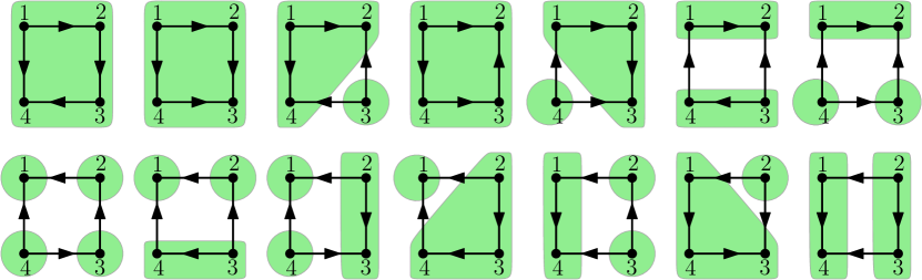
Figure 2. The source-components of the 14 acyclic orientations of the graph of Figure 1.

Proposition 4.2 ([7, Theorem 7.4]).

Let $G=([n],E)$ be a graph, and let $i$ be a non-negative integer. Then, $(-1)^{n-i}[q^{i}]\chi_{G}(q)$ is the number of acyclic orientations of $G$ with exactly $i$ source-components. In particular, $(-1)^{n-1}[q^{1}]\chi_{G}(q)$ is the number of acyclic orientations with single source 1.

Example 4.3.

The graph $G$ in Figure 1, has 1 (resp. 4, 6, 3) acyclic orientations with 4 (resp. 3, 2, 1) source-components. This matches the coefficients of $\chi_{G}(q)=q^{4}-4q3+6q2-3q$.

As we now explain, Proposition 4.2 is equivalent to the case $j=0$ of Theorem 1.1. Let $\mathcal{A}_{i}$ be the set of acyclic orientations of $G$ with exactly $i$ source-components. Let $\gamma\in\mathcal{A}_{i}$, and let $S_{1},\ldots,S_{i}$ be its source-components. The sets $S_{1},\ldots,S_{i}$ clearly satisfy

• $S_{1},\ldots,S_{i}$ are disjoint sets and $\bigcup_{k=1}^{i}S_{k}=[n]$,

• for all $k\in[i]$ the restriction $\gamma_{k}$ of $\gamma$ to the subgraph $G[S_{k}]$ is an acyclic orientation with single source $\min(S_{k})$,

• for all $\ell>k$, any edge between $S_{k}$ and $S_{\ell}$ is directed toward its endpoint in $S_{k}$.

• $\min(S_{1})<\min(S_{2})<\cdots<\min(S_{i})$,

These conditions are easily seen to be sufficient: an acyclic orientation $\gamma$ has source-components $S_{1},\ldots,S_{i}$ if and only if the conditions (i-iv) hold. Moreover, the tuple $((S_{1},\gamma_{1}),\ldots,(S_{i},\gamma_{i}))$ uniquely determines $\gamma\in\mathcal{A}_{i}$. Hence, Proposition 4.2 can be interpreted as stating that $(-1)^{n-i}[q^{i}]\chi_{G}(q)$ is the number of tuples $((S_{1},\gamma_{1}),\ldots,(S_{i},\gamma_{i}))$ satisfying (i-iv). Upon permuting the indices $\{1,\ldots,i\}$, we get that $i!(-1)^{n-i}[q^{i}]\chi_{G}(q)$ is the number of tuples $((S_{1},\gamma_{1}),\ldots,(S_{i},\gamma_{i}))$ satisfying conditions (i-iii), which is exactly the case $j=0$ of Theorem 1.1.

It is not hard to combine the above discussions to show that Theorem 1.1 is equivalent to the following statement.

Corollary 4.4.

Let $G$ be a graph, let $q$ be an indeterminate, and let $i,j$ be non-negative integers. Then $(-1)^{n-i}[q^{i}]\chi_{G}(q-j)$ is the number of pairs $(\gamma,f)$, where $\gamma$ is an acyclic orientation of $G$, and $f$ is a $(j+1)$-coloring of $G$ without $\gamma$-descent, such that the restriction $\gamma_{1}$ of $\gamma$ to the subgraph $G[f^{-1}(1)]$ has exactly $i$ source-components (with the special case $i=0$ corresponding to $f^{-1}(1)=\emptyset$).

4.2. Generalization of Theorem 1.1 and relation to results by Gessel and Lass.

In this subsection we establish a generalization of Theorem 1.1, which extends results from Gessel [6] and Lass [9].

Theorem 4.5.

Let $G=([n],E)$ be a graph. Let $d$ be a non-negative integer such that the vertices $1,2,\ldots,d$ are pairwise adjacent. Let $q$ be an indeterminate, and let

(12) $${\widehat{\chi}_{d}}(q):=\frac{\chi_{G}(q)}{q(q-1)\cdots(q-d+1)},$$

with the special case $d=0$ being interpreted as ${\widehat{\chi}_{0}}(q)=\chi_{G}(q)$. Then ${\widehat{\chi}_{d}}(q)$ is a polynomial in $q$ such that for all non-negative integers $i,j$, the evaluation $(-1)^{n-d-i}\,{\widehat{\chi}_{d}}^{(i)}(-j)$ is the number of tuples $((V_{1},\gamma_{1}),\ldots,(V_{d+i+j},\gamma_{d+i+j}))$ such that

• $V_{1},\ldots,V_{d+i+j}$ are disjoint subsets of vertices, such that $\bigcup_{k}V_{k}=[n]$, and for all $k\in[d]$, $k\in V_{k}$,

• for all $k\in[d+i+j]$, $\gamma_{k}$ is an acyclic orientation of $G[V_{k}]$, and if $k\leq d+i$ then $V_{k}\neq\emptyset$ and $\gamma_{k}$ has a unique source which is the vertex $\min(V_{k})$.

Observe that the case $d=0$ of Theorem 4.5 is Theorem 1.1. The special case $i=0$ for $d\in\{1,2\}$ was obtained by Gessel in [6, Thm 3.3 and 3.4].

Example 4.6.

For the graph $G$ represented in Figure 2, we have ${\widehat{\chi}_{2}}(q)=q^{2}-3q+3$. Theorem 4.5 in the case $d=2,i=1,j=0$ (correctly) predicts that there are exactly $-{\widehat{\chi}_{2}}^{\prime}(0)=3$ triples $((V_{1},\gamma_{1}),(V_{2},\gamma_{2}),(V_{3},\gamma_{3}))$, such that $1\in V_{1}$, $2\in V_{2}$, $V_{1}\uplus V_{2}\uplus V_{3}=[4]$, and for all $k\in[3]$, $\gamma_{k}$ is an acyclic orientation of $G[V_{k}]$ with unique source $\min(V_{k})$.

Proof.

Since the vertices $1,2,\ldots,d$ are pairwise adjacent, we know that $\chi_{G}(k)=0$ for all $k\in\{0,\ldots,d-1\}$. Since these integers are roots of $\chi_{G}(q)$, this polynomial is divisible by $q(q-1)\cdots(q-d+1)$. Hence ${\widehat{\chi}_{d}}(q)$ is a polynomial. We now prove the interpretation of $(-1)^{n-d-i}{\widehat{\chi}_{d}}^{(i)}(-j)$. Fix an integer $q>d$. Note that in any proper $q$-coloring of $G$, the vertices $1,\ldots,d$ have distinct colors in $[q]$. So it is easy to see that ${\widehat{\chi}_{d}}(q)$ can be interpreted as the number of proper $q$-colorings such that for all $k$ in $[d]$ the vertex $k$ has color $k$. In other words, for all $k\in[d]$, the $q$-colorings counted by ${\widehat{\chi}_{d}}(q)$ are such that the set of vertices colored $k$ are independent sets containing the vertex $k$. Thus, reasoning as in the proof of (6), we get the following expression of ${\widehat{\chi}_{d}}(q)$ in terms of trivial heaps:

(13) $${\widehat{\chi}_{d}}(q)=[x_{1}\cdots x_{n}]\left(\prod_{k=1}^{d}\frac{T_{k}(\mathbf{x})}{T(\mathbf{x})}\right)T(\mathbf{x})^{q},$$

where $T_{k}(\mathbf{x})=\sum_{\mathbf{h}\in\mathcal{T}_{k}}\mathbf{x}^{\mathbf{h}}$ and $\mathcal{T}_{k}$ is the set of trivial heaps containing a piece of type $k$. Again, this equation holds for an indeterminate $q$, because both sides are polynomials in $q$. Differentiating (13) with respect to $q$ ($i$ times), and setting $q=-j$ gives

$$(-1)^{n-d-i}\,{\widehat{\chi}_{d}}^{(i)}(-j)=[x_{1}\cdots x_{n}]\left(\prod_{k=1}^{d}-\frac{T_{k}(-\mathbf{x})}{T(-\mathbf{x})}\right)\left(-\ln(T(-\mathbf{x}))\right)^{i}\left(\frac{1}{T(-\mathbf{x})}\right)^{j}.$$

By Lemma 2.5, $\displaystyle-\frac{T_{k}(-\mathbf{x})}{T(-\mathbf{x})}=\frac{T_{\overline{\{k\}}}(-\mathbf{x})}{T(-\mathbf{x})}-1=H_{\{k\}}(\mathbf{x})-1,$ which together with Theorem 2.4 gives

(14) $$(-1)^{n-d-i}{\widehat{\chi}_{d}}^{(i)}(-j)=[x_{1}\cdots x_{n}]\left(\prod_{k=1}^{d}H_{\{k\}}(\mathbf{x})-1\right)\cdot P(\mathbf{x})^{i}\cdot H(\mathbf{x})^{j}.$$

Observe that for any sets of vertices $S,V\subseteq[n]$, the coefficient $[\mathbf{x}^{V}]H_{S}(\mathbf{x})$ is the number of acyclic orientations of $G[V]$ whose sources are all in $S$. Hence, for any set $V\subseteq[n]$,

$$[\mathbf{x}^{V}]\left(H_{\{k\}}(\mathbf{x})-1\right)=\left|\begin{array}[]{ll}\#\textrm{ acyclic orientations of }G[V]\textrm{ with unique source }k,\textrm{ if }k\in V,\\[2.84526pt] 0\textrm{ otherwise}.\end{array}\right.$$

Using this together with Lemma 3.3, we see that (14) gives the claimed interpretation of $(-1)^{n-d-i}\,{\widehat{\chi}_{d}}^{(i)}(-j)$. ∎

Theorem 4.5 could equivalently be stated as giving an interpretation for the coefficients of the polynomial ${\widehat{\chi}_{d}}(q-j)$ for all $j,d\geq 0$. We will next give an interpretation for the coefficients of ${\widehat{\chi}_{d}}(q+1)$ for all $d>0$.

Let us first recall a classical result of Crapo [2]. Let $u,v$ be two adjacent vertices of a graph $G$. An acyclic orientation of $G$ is called $(u,v)$-bipolar if it has unique source $u$ and unique sink $v$. A classical result of Crapo [2] is that $(-1)^{n}[q^{1}]{\widehat{\chi}_{1}}(q+1)$ is the number of $(u,v)$-bipolar orientations of $G$ (which is independent of $u,v$). We mention that, for a connected graph, ${\widehat{\chi}_{1}}(q+1)$ is related to the Tutte polynomial $T_{G}(x,y)$ by ${\widehat{\chi}_{1}}(q+1)=(-1)^{n-1}T_{G}(-q,0)$, hence $(-1)^{n}[q^{1}]{\widehat{\chi}_{1}}(q+1)=[x^{1}y^{0}]T_{G}(x,y)$. Crapo’s result was recovered using the theory of heaps in [6, Thm 3.1]. In Lass [9, Thm 5.2], an interpretation was given for every coefficient of the polynomial ${\widehat{\chi}_{1}}(q+1)$ for a connected graph $G$. Following this lead, we obtain the following result for connected graphs having a set of $d$ pairwise adjacent vertices.

Theorem 4.7.

Let $G=([n],E)$ be a connected graph. Let $d$ be a positive integer such that the vertices $1,2,\ldots,d$ are pairwise adjacent. Let $q$ be an indeterminate, and let ${\widehat{\chi}_{d}}(q)$ be the polynomial defined by (12). Upon relabeling the vertices of $G$, one can assume that for all $k>1$ the vertex labeled $k$ is adjacent to a vertex of label less than $k$. Then for all $i\geq 0$, $(-1)^{n-d-i}[q^{i}]{\widehat{\chi}_{d}}(q+1)$ is the number of acyclic orientations of $G$ having exactly $d+i$ source-components such that the vertices $1,2,\ldots,d$ are in different source-components and $1$ is the unique sink.

Note that for the orientations described in Theorem 4.7, the vertex 1 is necessarily alone in its source-component. In particular, in the special case $d=1$, and $i=1$ the orientations described have unique sink 1 and unique source 2, which gives Crapo’s interpretation of $(-1)^{n}[q^{1}]{\widehat{\chi}_{1}}(q+1)$ as counting $(2,1)$-bipolar orientations. The case $d=1$ of Theorem 4.7 is exactly [9, Thm 5.2]. The case $d=2$ is equivalent to the case $d=1$ (because ${\widehat{\chi}_{1}}(q+1)=q\,{\widehat{\chi}_{2}}(q+1)$ and the vertices 1, 2 are necessarily in different source-components). The cases $d\geq 3$ are new.

Proof.

Let $R_{d}(q)={\widehat{\chi}_{d}}(q+1)$, and let $c_{i}=[q^{i}]{\widehat{\chi}_{d}}(q+1)=[q^{i}]R_{d}(q)=\frac{R^{(i)}(0)}{i!}$. By (13),

$$R_{d}(q)=[x_{1}\cdots x_{n}]\,T_{1}(\mathbf{x})\left(\prod_{k=2}^{d}\frac{T_{k}(\mathbf{x})}{T(\mathbf{x})}\right)T(\mathbf{x})^{q},$$

for an indeterminate $q$. After differentiating with respect to $q$ ($i$ times) one gets

$$(-1)^{n-d-i}c_{i}=[x_{1}\cdots x_{n}]\,\left(-T_{1}(-\mathbf{x})\right)\left(\prod_{k=2}^{d}-\frac{T_{k}(-\mathbf{x})}{T(-\mathbf{x})}\right)\frac{\left(-\ln(T(-\mathbf{x}))\right)^{i}}{i!}.$$

Reasoning as in the proof of Theorem 4.5 this gives:

$$(-1)^{n-d-i}c_{i} = [x_{1}\cdots x_{n}]\left(-T_{1}(-\mathbf{x})\right)\left(\prod_{k=2}^{d}(H_{\{k\}}(\mathbf{x})-1)\right)\,\frac{P(\mathbf{x})^{i}}{i!},$$

$$= \sum_{U\subseteq[n]}[\mathbf{x}^{U}]\left(-T_{1}(-\mathbf{x})\right)\cdot[\mathbf{x}^{\overline{U}}]\left(\prod_{k=2}^{d}(H_{\{k\}}(\mathbf{x})-1)\right)\frac{P(\mathbf{x})^{i}}{i!},$$

where $\overline{U}:=[n]\setminus U$.

For $V\subseteq[n]\setminus\{1\}$, let $\mathcal{S}_{V}\equiv\mathcal{S}_{V}(d,i)$ be the set of acyclic orientations of $G[V]$ having $d+i-1$ source-components, such that $2,\ldots,d$ are in different source-components (with $\mathcal{S}_{V}=\emptyset$ whenever $V$ does not contain $\{2,\ldots,d\}$). Reasoning as before, we see that $|\mathcal{S}_{V}|=\displaystyle[\mathbf{x}^{V}]\left(\prod_{k=2}^{d}(H_{\{k\}}(\mathbf{x})-1)\right)\frac{P(\mathbf{x})^{i}}{i!}$. Hence, using the fact that $T_{1}$ is the generating function of the set $I$ of independent sets of $G$ containing the vertex 1, we get

(15) $$(-1)^{n-d-i}c_{i}=\sum_{U\in I}(-1)^{|U|-1}|\mathcal{S}_{\overline{U}}|.$$

We will now simplify this expression by defining a sign-reversing involution $\phi$ on the set $\mathcal{S}:=\{(U,\gamma)~{}|~{}U\in I,~{}\gamma\in\mathcal{S}_{\overline{U}}\}$. Given $(U,\gamma)\in\mathcal{S}$ consider the orientation $\overline{\gamma}$ which is the extension of $\gamma$ to the full graph $G$ obtained by orienting every edge incident to a vertex $u\in U$ toward $u$. It is not hard to see that $\overline{\gamma}$ has $d+i$ source-components $S_{1},\ldots,S_{d+i}$, such that $S_{1}=\{1\}$ and $S_{2}\setminus U,\ldots,S_{d+i}\setminus U$ are the source-components of $\gamma$. Indeed, it is clear that the first source-component $S_{1}$ is $\{1\}$ because 1 is a sink, and moreover no vertex $u\in U\setminus\{1\}$ can be the source of a source-component because $u$ is adjacent to a vertex with smaller label.

We now define $\phi$ on $\mathcal{S}$. Let $(U,\gamma)\in\mathcal{S}$, and let $Z$ be the set of sinks of $\overline{\gamma}$. Note that $U\subseteq Z$ and $Z\in I$. If $Z=\{1\}$, then define $\phi(U,\gamma)=(U,\gamma)$. Otherwise we set $s=\min(Z\setminus\{1\})$ and consider two cases. If $s\in U$, we define $\phi(U,\gamma)=(U\setminus\{s\},\gamma^{\prime})$, where $\gamma^{\prime}$ is the extension of $\gamma$ to $G[\overline{U}\cup\{s\}]$ obtained by orienting every edge incident to $s$ toward $s$. If $s\notin U$, we define $\phi(U,\gamma)=(U\cup\{s\},\gamma^{\prime})$, where $\gamma^{\prime}$ is the restriction of $\gamma$ to $G[\overline{U}\setminus\{s\}]$.

We know from the above discussion that in every case $\phi(U,\gamma)\in\mathcal{S}$. Moreover it is clear that $\phi$ is an involution (because the orientation $\overline{\gamma}$ is unchanged by $\phi$), and that if $Z\neq\{1\}$, the contribution of the pairs $(U,\gamma)$ and $\phi(U,\gamma)$ to the right-hand side of (15) will cancel out. Hence, the right-hand side of (15) is the cardinality of the set $\mathcal{S}^{\prime}$ of pairs $(U,\gamma)\in\mathcal{S}$ such that $Z=U=\{1\}$. This gives the claimed interpretation of $(-1)^{n-d-i}c_{i}$ (upon identifying each element $(\{1\},\gamma)$ in $\mathcal{S}^{\prime}$ with the orientation $\overline{\gamma}$ of $G$ which is the extension of $\gamma$ to $G$ obtained by orienting every edge incident to $1$ toward $1$). ∎

5. Chromatic symmetric function

In this section we consider the chromatic symmetric function defined by Stanley in [11], and we obtain a symmetric function refinement of Theorem 1.1, as well as a “superfication” extension.

Let $G=([n],E)$ be a graph. We consider colorings of $G$ with colors in the set $\mathbb{P}:=\{1,2,3,\ldots\}$ of positive integers. A function $f:V\to\mathbb{P}$ is called $\mathbb{P}$-coloring, and as before $f$ is said to be proper if adjacent vertices get different colors. Let $\mathbf{z}=(z_{1},z_{2},\ldots)$ be a set of variables indexed by $\mathbb{P}$. The chromatic symmetric function of $G$ is the generating function of its proper $\mathbb{P}$-colorings counted according to the number of times each color is used:

$$X_{G}(\mathbf{z})=\sum_{f\textrm{ proper }\mathbb{P}\textrm{-coloring}}~{}~{}~{}\prod_{v\in[n]}z_{f(v)}.$$

Observe that $X_{G}(\mathbf{z})$ is a homogeneous symmetric function of degree $n$ in $\mathbf{z}$, and that for every positive integer $j$,

(16) $$X_{G}(\mathbf{1}^{j})=\chi_{G}(j),$$

where $\mathbf{1}^{j}$ is the evaluation obtained by setting $z_{i}=1$ for all $i\in[j]$, and $z_{i}=0$ for all $i>j$.

Example 5.1.

For the graph $G$ represented in Figure 1, the chromatic symmetric function is easily seen to be

$$X_{G}(\mathbf{z}) =24\sum_{1\leq i<j<k<l}z_{i}z_{j}z_{k}z_{l}+4\sum_{1\leq i<j<k}(z_{i}^{2}z_{j}z_{k}+z_{i}z_{j}^{2}z_{k}+z_{i}z_{j}z^{2}_{k})+2\sum_{1\leq i<j}z_{i}^{2}z_{j}^{2}$$

In particular, one gets

$$X_{G}(\mathbf{1}^{j})=24\binom{j}{4}+12\binom{j}{3}+2\binom{j}{2}=j^{4}-4j^{3}+6j^{2}-3j,$$

which indeed coincides with the expression of $\chi_{G}(j)$ given in the caption of Figure 1.

In [11, 12] Stanley establishes many beautiful properties of $X_{G}$. Our goal is to recover and extend some of these results using the machinery of heaps. The starting point is the symmetric function analogue of Lemma 3.2:

(17) $$X_{G}(\mathbf{z})=[x_{1}\cdots x_{n}]\prod_{i=1}^{\infty}T(z_{i}\mathbf{x}),$$

where $T(\mathbf{x})$ is the generating function of trivial $G$-heaps.

We first discuss the result of applying the duality mapping to $X_{G}$. We recall some basic definitions. For a field $K$ of characteristic $0$, we denote by $\mathop{Sym}_{K}(\mathbf{z})$ the algebra of symmetric functions in $\mathbf{z}$, with coefficients in $K$. Hence, $X_{G}(\mathbf{z})\in\mathop{Sym}_{\mathbb{Q}}(\mathbf{z})\subseteq\mathop{Sym}_{K}(\mathbf{z})$. Let $e_{k},h_{k},p_{k}$ be the elementary, complete and power-sum symmetric functions, which are defined by $e_{0}=h_{0}=p_{0}=1$, and for $k\in\mathbb{P}$,

$$e_{k}=\sum_{i_{1}<\cdots<i_{k}\in\mathbb{P}}z_{i_{1}}\cdots z_{i_{k}},~{}\quad h_{k}=\sum_{i_{1}\leq\cdots\leq i_{k}\in\mathbb{P}}z_{i_{1}}\cdots z_{i_{k}},~{}~{}\textrm{and}~{}\quad p_{k}=\sum_{i\in\mathbb{P}}z_{i}^{k}.$$

Recall that $\mathop{Sym}_{K}(\mathbf{z})$ is generated freely as a commutative $K$-algebra by each of these sets of symmetric functions. In other words, if $(g_{k})_{k\geq 1}$ stands for any one of these families, then $(g_{\lambda})_{\lambda}$ forms a basis of $\mathop{Sym}_{K}(\mathbf{z})$, where $\lambda=(\lambda_{1},\ldots,\lambda_{k})$ runs through all integer partitions and $g_{\lambda}:=g_{\lambda_{1}}\cdots g_{\lambda_{k}}$. Lastly, the duality mapping $\omega\equiv\omega_{\mathbf{z}}$ is defined as the algebra homomorphism of $\mathop{Sym}_{K}(\mathbf{z})$ such that $\omega(e_{k})=h_{k}$. As is well known, $\omega$ also satisfies $\omega(h_{k})=e_{k}$ and $\omega(p_{k})=(-1)^{k-1}p_{k}$. The following result is [11, Thm 4.2], and we give an alternative proof.

Proposition 5.2 ([11]).

With the above notation,

$$\omega(X_{G})(\mathbf{z})=\sum_{(\gamma,f)}~{}\prod_{v\in[n]}z_{f(v)},$$

where the sum is over the set $\mathcal{C}$ of pairs $(\gamma,f)$ where $\gamma$ is an acyclic orientation of $G$ and $f$ is a $\mathbb{P}$-coloring without $\gamma$-descent.

Proof.

We claim that

(18) $$\omega\left(\prod_{i=1}^{\infty}T(z_{i}\mathbf{x})\right)=\prod_{i=1}^{\infty}H(z_{i}\mathbf{x}).$$

Here and in the following we are actually extending $\omega$ to the larger space of symmetric power series in $\mathbf{z}$ with coefficients in $K$ (in other words, we allow for symmetric functions of infinite degree), and we can take $K$ to be the field $\mathbb{Q}(\mathbf{x})$ of rational functions in $\mathbf{x}$ with rational coefficients. Observe that for any scalar $t$ in the underlying field $K$,

$$\omega\left(\prod_{i=1}^{\infty}(1+t\,z_{i})\right)=\omega\left(\sum_{k=0}^{\infty}e_{k}t^{k}\right)=\sum_{k=0}^{\infty}h_{k}t^{k}=\prod_{i=1}^{\infty}\frac{1}{1-t\,z_{i}}.$$

Now let $Q(Z)\in K[Z]$ be a polynomial such that $Q(0)=1$. Working in the algebraic closure $\overline{K}$ of $K$, one can write $Q(Z)=\prod_{k=1}^{d}(1+t_{k}Z)$ with $t_{1},\ldots,t_{d}\in\overline{K}$. Then, still working over $\overline{K}$, one gets

$$\omega\left(\prod_{i=1}^{\infty}Q(z_{i})\right)=\prod_{k=1}^{d}\omega\left(\prod_{i=1}^{\infty}(1+t_{k}z_{i})\right)=\prod_{k=1}^{d}\prod_{i=1}^{\infty}\frac{1}{1-t_{k}z_{i}}=\prod_{i=1}^{\infty}\frac{1}{Q(-z_{i})}.$$

Applying this identity to the polynomial $Q(Z):=T(Z\mathbf{x})$ gives (18). Hence,

(19) $$\omega(X_{G})(\mathbf{z}) = \omega\left([x_{1}\cdots x_{n}]\prod_{i=1}^{\infty}T(z_{i}\mathbf{x})\right)=[x_{1}\cdots x_{n}]\,\omega\!\left(\prod_{i=1}^{\infty}T(z_{i}\mathbf{x})\right)$$

$$= [x_{1}\cdots x_{n}]\prod_{i=1}^{\infty}H(z_{i}\mathbf{x}).$$

Expanding the right-hand side of Equation (19), we obtain that $\omega(X_{G})(\mathbf{z})$ is the sum of the monomials $z_{1}^{|V_{1}|}z_{2}^{|V_{2}|}\cdots$ over all infinite sequences $((V_{1},\gamma_{1}),(V_{2},\gamma_{2}),\ldots)$, where $V$ is the disjoint union of the sets $V_{i}$ and $\gamma_{i}$ is an acyclic orientation on $G[V_{i}]$ for all $i\in\mathbb{P}$. Now Proposition 5.2 follows using the correspondence detailed after Proposition 4.1. ∎

For an acyclic orientation $\gamma$ of $G$ with source-components $S_{1},\ldots,S_{k}$, we denote $\lambda(\gamma)$ the partition of $n$ obtained by ordering the sizes $|S_{i}|$ in a weakly decreasing manner.

Proposition 5.3.

With the above notation,

$$X_{G}(\mathbf{z})=(-1)^{n}\sum_{\gamma\in\mathcal{A}}(-1)^{\ell(\lambda(\gamma))}p_{\lambda(\gamma)},$$

where the sum is over the set $\mathcal{A}$ of acyclic orientations of $G$, and $\ell(\lambda(\gamma))$ is the number of source-components of $\gamma$. Equivalently,

(20) $$\omega(X_{G})(\mathbf{z})=\sum_{\gamma\in\mathcal{A}}p_{\lambda(\gamma)}.$$

Example 5.4.

For the graph $G$ in Figure 2, the chromatic symmetric function is given in Example 5.1, and one can compute

$$X_{G}(\mathbf{z}) = p_{1,1,1,1}-4p_{2,1,1}+4p_{3,1}+2p_{2,2}-3p_{4};$$

$$\omega(X_{G})(\mathbf{z}) = p_{1,1,1,1}+4p_{2,1,1}+4p_{3,1}+2p_{2,2}+3p_{4}.$$

As stated in Theorem 5.3, the coefficients obtained in this expansions correspond to the fact that the number of acyclic orientations $\gamma$ of $G$ with partition $\lambda(\gamma)$ equal to $(1,1,1,1)$ (resp. $(2,1,1)$, $(3,1)$, $(2,2)$, $(4)$) is 1 (resp. 4, 4, 2, 3). This matches the direct count one can do by looking at Figure 2.

Proof.

It suffices to prove (20), since the other identity follows by applying $\omega$. Recall from Theorem 2.4, that $\displaystyle H(\mathbf{x})=\exp(P(\mathbf{x})):=\sum_{k=0}^{\infty}\frac{P(\mathbf{x})^{k}}{k!}$, where $P$ is the generating function of $G$-pyramids. This gives

$$\prod_{i=1}^{\infty}H(z_{i}\mathbf{x}) = \exp\!\left(\sum_{i=1}^{\infty}P(z_{i}\mathbf{x})\right)~{}=~{}\exp\!\left(\sum_{\mathbf{h}\in\mathcal{P}}\frac{p_{{|\mathbf{h}|}}}{{|\mathbf{h}|}}\mathbf{x}^{\mathbf{h}}\right)~{}=~{}\exp\!\left(\sum_{\mathbf{m}\in\mathbb{N}^{n}}|\mathcal{B}_{\mathbf{m}}|\frac{p_{|\mathbf{m}|}}{|\mathbf{m}|}\mathbf{x}^{\mathbf{m}}\right).$$

where for $\mathbf{m}=(m_{1},\ldots,m_{n})$ we denote $|\mathbf{m}|=\sum_{i}m_{i}$, and we let $\mathcal{B}_{\mathbf{m}}$ be the set of $G$-pyramids of type $\mathbf{m}$. Hence

(21) $$\prod_{i=1}^{\infty}H(z_{i}\mathbf{x}) = \prod_{\mathbf{m}\in\mathbb{N}^{n}}\exp\!\left(|\mathcal{B}_{\mathbf{m}}|\,\frac{p_{|\mathbf{m}|}}{|\mathbf{m}|}\mathbf{x}^{\mathbf{m}}\right).$$

Thus, by (19),

$$\omega(X_{G})(\mathbf{z}) = [x_{1}\cdots x_{n}]\prod_{\mathbf{m}\in\{0,1\}^{n}}\exp\!\left(|\mathcal{B}_{\mathbf{m}}|\,\frac{p_{|\mathbf{m}|}}{|\mathbf{m}|}\mathbf{x}^{\mathbf{m}}\right)$$

$$= [x_{1}\cdots x_{n}]\prod_{\mathbf{m}\in\{0,1\}^{n}}\left(1+|\mathcal{B}_{\mathbf{m}}|\,\frac{p_{|\mathbf{m}|}}{|\mathbf{m}|}\mathbf{x}^{\mathbf{m}}\right).$$

For $V\subseteq[n]$, let $\mathcal{B}_{V}$ be the set of acyclic orientations of $G[V]$ with unique source $\min(V)$ (with the convention $\mathcal{B}_{\emptyset}=\emptyset$). By Lemma 3.3, $|\mathcal{B}_{V}|=\frac{|\mathcal{B}_{\mathbf{m}}|}{|\mathbf{m}|}$ if $V\neq\emptyset$, where $\mathbf{m}\in\{0,1\}^{n}$ is the tuple encoding the set $V$. Hence

$$\omega(X_{G})(\mathbf{z})=[x_{1}\cdots x_{n}]\prod_{V\subseteq[n]}\left(1+|\mathcal{B}_{V}|\,p_{|V|}\mathbf{x}^{V}\right)=\sum_{\{(V_{1},\gamma_{1}),\ldots,(V_{i},\gamma_{i})\}}~{}\prod_{k=1}^{i}p_{|V_{k}|},$$

where the sum is over the set $\mathcal{B}$ of sets of pairs $\{(V_{1},\gamma_{1}),\ldots,(V_{i},\gamma_{i})\}$ such that $V_{1},\ldots,V_{i}$ form a set partition of $[n]$, and for all $k\in[i]$ $\gamma_{k}$ is in $\mathcal{B}_{V_{k}}$. Reasoning as in Section 4.1, we can identify $\mathcal{B}$ with the set of acyclic orientations and the sets $V_{i}$ with the corresponding source-components. This proves (20). ∎

Remark 5.5.

Proposition 5.3 could alternatively be obtained by combining [11, Theorem 2.6] with [7, Theorem 7.3]. Indeed, [11, Theorem 2.6] expresses the coefficient of $p_{\lambda}$ in $X_{G}$ in terms of the Möbius function of the bond lattice of $G$, and [7, Theorem 7.3] shows that this Möbius function has the combinatorial interpretation given in Proposition 5.3.

As we now explain, Propositions 5.2 and 5.3 are refinements of Propositions 4.1 and 4.2 respectively. Let $q$ be an indeterminate, and let $X_{G}(\mathbf{z})_{|\forall k>0,~{}p_{k}=q}$ denote the polynomial in $q$ obtained by substituting each of the generators $p_{1},p_{2},\ldots$ by $q$. We observe that

(22) $$X_{G}(\mathbf{z})_{|\forall k>0,~{}p_{k}=q}=\chi_{G}(q)$$

and for any non-negative integer $j$,

(23) $$\omega(X_{G})(\mathbf{1}^{j})=(-1)^{n}\chi_{G}(-j).$$

Indeed the polynomials in (22) coincide on positive integers by (16) (since $p_{k}(\mathbf{1}^{j})=j$), and $\omega(X_{G})(\mathbf{1}^{j})=(-1)^{n}X_{G}(\mathbf{z})_{|\forall k>0,~{}p_{k}=-j}$ (since $\omega(p_{k})=-(-1)^{k}p_{k}$ and $X_{G}$ is homogeneous of degree $n$). Thus, specializing Proposition 5.2 at $\mathbf{z}=\mathbf{1}^{j}$ gives Proposition 4.1, and specializing Proposition 5.3 at $(p_{1},p_{2},\ldots)=(q,q,\ldots)$ gives Proposition 4.2.

We now give a refinement of Theorem 1.1. Consider a second set of variables $\mathbf{y}=(y_{1},y_{2},\ldots)$. For a symmetric function $f=f(\mathbf{z})$, we denote $f(\mathbf{y}+\mathbf{z})$ the symmetric function in $\mathbf{y}$ and $\mathbf{z}$ obtained by substituting the variable $z_{2i-1}$ by $y_{i}$ and $z_{2i}$ by $z_{i}$ for all $i\in\mathbb{P}$ (equivalently, substituting the generator $p_{i}=p_{i}(\mathbf{z})$ by $p_{i}(\mathbf{y})+p_{i}(\mathbf{z})$).

Theorem 5.6.

Let $G$ be a graph. Let $\mathcal{D}$ be the set of pairs $(\gamma,f)$, where $\gamma$ is an acyclic orientation of $G$ and $f:V\to\mathbb{N}$ is an $\mathbb{N}$-coloring of $G$ without $\gamma$-descent. Then

$$\omega(X_{G})(\mathbf{y}+\mathbf{z})=\sum_{(\gamma,f)\in\mathcal{D}}\,p_{\lambda(\gamma_{0})}(\mathbf{y})\,\prod_{i\in\mathbb{P}}z_{i}^{|f^{-1}(i)|}$$

where $\gamma_{0}$ is the restriction of $\gamma$ to $G[f^{-1}(0)]$.

Observe that Corollary 4.4 (which is equivalent to Theorem 1.1) is the specialization of Theorem 5.6 obtained by substituting $p_{k}(\mathbf{y})$ by $q$ and $p_{k}(\mathbf{z})$ by $j$ for all $k\in\mathbb{P}$, and then taking the coefficient of $q^{i}$. Observe also that setting $\mathbf{y}=0$ in Theorem 5.6 gives Proposition 5.2, while setting $\mathbf{z}=0$ gives Proposition 5.3.

Proof.

By (19),

$$\omega(X_{G})(\mathbf{y}+\mathbf{z}) = [x_{1}\cdots x_{n}]\left(\prod_{i=1}^{\infty}H(y_{i}\mathbf{x})\right)\cdot\left(\prod_{i=1}^{\infty}H(z_{i}\mathbf{x})\right),$$

$$= \sum_{U\uplus V=[n]}\left([\mathbf{x}^{U}]\prod_{i=1}^{\infty}H(y_{i}\mathbf{x})\right)\cdot\left([\mathbf{x}^{V}]\prod_{i=1}^{\infty}H(z_{i}\mathbf{x})\right).$$

where the sum is over the pairs $(U,V)$ of disjoint sets whose union is $[n]$. Applying (19) to the induced graphs $G[U]$ and $G[V]$ gives

$$\omega(X_{G})(\mathbf{y}+\mathbf{z}) = \sum_{U\uplus V=[n]}\omega(X_{G[U]})(\mathbf{y})\cdot\omega(X_{G[V]})(\mathbf{z}).$$

Lastly, applying Propositions 5.3 and 5.2 to $\omega(X_{G[U]})(\mathbf{y})$ and $\omega(X_{G[V]})(\mathbf{z})$ respectively gives

$$\omega(X_{G})(\mathbf{y}+\mathbf{z}) = \sum_{U\uplus V=[n]}\left(\sum_{\gamma_{0}\in\mathcal{A}(U)}p_{\lambda(\gamma_{0})}(\mathbf{y})\right)\cdot\left(\sum_{(\gamma^{\prime},f^{\prime})\in\mathcal{C}(V)}~{}\prod_{v\in V}z_{f^{\prime}(v)}\right),$$

where $\mathcal{A}(U)$ is the set of acyclic orientations of $G[U]$, and $\mathcal{C}(V)$ is the set of pairs $(\gamma^{\prime},f^{\prime})$ with $\gamma^{\prime}$ acyclic orientation of $G[V]$ and $f^{\prime}$ a $\mathbb{P}$-coloring of $G[V]$ without $\gamma^{\prime}$-descent. Theorem 5.6 follows by identifying $\bigcup_{U\uplus V=[n]}\mathcal{A}(U)\times\mathcal{C}(V)$ with $\mathcal{D}$ (identifying $U$ with the set $\gamma^{-1}(0)$ of vertices colored 0, etc.). ∎

As the proof of Theorem 5.6 shows, it is easy to combine several results into one, at the cost of using several sets of variables. This is because our identities hold at the level of the heap generating function $\prod_{i=1}^{\infty}T(z_{i}\mathbf{x})$. For instance, it is straightforward to recover the superfication result [11, Thm 4.3], as we now explain.

We denote by $X_{G}(\mathbf{y}-\mathbf{z})$ the function of $\mathbf{y}$ and $\mathbf{z}$ obtained from $X_{G}(\mathbf{z})$ by substituting $p_{k}(\mathbf{z})$ by $p_{k}(\mathbf{y})-(-1)^{k}p_{k}(\mathbf{z})$. Equivalently, $X_{G}(\mathbf{y}-\mathbf{z})$ is obtained from $X_{G}(\mathbf{y}+\mathbf{z})$ by applying duality only on the $\mathbf{z}$ variables:

$$X_{G}(\mathbf{y}-\mathbf{z}):=\omega_{\mathbf{z}}(X_{G}(\mathbf{y}+\mathbf{z})).$$

Using (17) and (18) gives

$$X_{G}(\mathbf{y}-\mathbf{z})=[x_{1}\cdots x_{n}]\left(\prod_{i=1}^{\infty}T(y_{i}\mathbf{x})\right)\cdot\left(\prod_{i=1}^{\infty}H(z_{i}\mathbf{x})\right)=\sum_{U\uplus V=[n]}X_{G[U]}(\mathbf{y})\cdot\omega(X_{G[V]})(\mathbf{z})$$

Hence,

$$X_{G}(\mathbf{y}-\mathbf{z})=\sum_{U\uplus V=[n]}\sum_{(f_{-},f_{+},\gamma_{+})}y_{i}^{|f_{-}^{-1}(i)|}\,z_{i}^{|f_{+}^{-1}(i)|},$$

where the inner sum is over the set of triples $(f_{-},f_{+},\gamma^{+})$ such that $f_{-}$ is a proper $\mathbb{P}$-coloring of $G[U]$, $\gamma_{+}$ is an acyclic orientation of $G[V]$, and $f_{+}$ is a $\mathbb{P}$-coloring of $G[V]$ without $\gamma_{+}$-descent. Equivalently (upon coloring $U$ with negative colors, and extending $\gamma_{+}$ to $G$), one gets

(24) $$X_{G}(\mathbf{y}-\mathbf{z})=\sum_{(\gamma,f)}\,\prod_{i\in\mathbb{P}}y_{i}^{|f^{-1}(-i)|}\,z_{i}^{|f^{-1}(i)|},$$

where the sum is over pairs $(\gamma,f)$ where $\gamma$ is an acyclic orientation of $G$ and $f:V\to\mathbb{Z}\setminus\{0\}$ is a coloring without $\gamma$-descent such that for all $i<0$ the vertices of color $i$ are pairwise non-adjacent. This is exactly [11, Thm 4.3].

There is no obstacle to pursuing this idea further. For instance, one can combine (24) and Theorem 5.6 into a single statement. Consider a new set of variables $\mathbf{z}^{\prime}=(z_{1}^{\prime},z_{2}^{\prime}\ldots)$, and the function $X_{G}(\mathbf{y}-(\mathbf{z}+\mathbf{z}^{\prime}))$ obtained from $X_{G}(\mathbf{z})$ by substituting $p_{k}(\mathbf{z})$ by $p_{k}(\mathbf{y})-(-1)^{k}(p_{k}(\mathbf{z})+p_{k}(\mathbf{z}^{\prime}))$. Let $\mathcal{E}$ be the set of pairs $(\gamma,f)$, where $\gamma$ is an acyclic orientation of $G$ and $f:V\to\mathbb{Z}$ is an $\mathbb{Z}$-coloring of $G$ without $\gamma$-descent, such that for all $i<0$ the vertices of color $i$ are pairwise non-adjacent. Then

(25) $$X_{G}(\mathbf{y}-(\mathbf{z}+\mathbf{z}^{\prime}))=\sum_{(\gamma,f)\in\mathcal{E}}\,p_{\lambda(\gamma_{0})}(\mathbf{z}^{\prime})\,\prod_{i\in\mathbb{P}}y_{i}^{|f^{-1}(-i)|}\,z_{i}^{|f^{-1}(i)|},$$

where $\gamma_{0}$ is the restriction of $\gamma$ to $G[f^{-1}(0)]$. Note that setting $\mathbf{y}=0$ in (25) gives Theorem 5.6, while setting $\mathbf{z}^{\prime}=0$ gives (24).

Remark 5.7.

Recall the notion of proper multicolorings from Remark 3.4. For $\mathbf{m}\in\mathbb{N}$, the symmetric function

(26) $$X_{G,\mathbf{m}}(\mathbf{z}):=[\mathbf{x}^{\mathbf{m}}]\prod_{i=1}^{\infty}T(z_{i}\mathbf{x}),$$

can be interpreted as counting proper multicolorings of $G$ of type $\mathbf{m}$ according to the number of times each color in $\mathbb{P}$ is used. By the same reasoning as in Remark 3.4, one gets

$$X_{G,\mathbf{m}}(\mathbf{z})=\frac{X_{G^{\mathbf{m}}}(\mathbf{z})}{\mathbf{m}!}.$$

so that these generalized chromatic symmetric functions are still chromatic symmetric functions, up to a multiplicative constant. Hence the results in this section apply to $X_{G,\mathbf{m}}$. This was noticed already in [12, Eq. (3)]. In fact [12, Proposition 2.1] follows from the combinatorial interpretation of (26).

Acknowledgment. We thank the anonymous referees for their numerous careful comments.

References

- [1] Pierre Cartier and Dominique Foata. Problèmes combinatoires de commutation et réarrangements. Lecture Notes in Mathematics, No. 85. Springer-Verlag, Berlin-New York, 1969.
- [2] Henry H. Crapo. A higher invariant for matroids. Journal of Combinatorial Theory, 2(4):406–417, 1967.
- [3] Bishal Deb. Chromatic polynomial and heaps of pieces. arXiv preprint arXiv:1902.02240., 2019.
- [4] Klaus Dohmen, André Pönitz, and Peter Tittmann. A new two-variable generalization of the chromatic polynomial. Discrete Math. Theor. Comput. Sci., 6(1):69–89, 2003.
- [5] Vesselin Gasharov. Incomparability graphs of -free posets are -positive. In Proceedings of the 6th Conference on Formal Power Series and Algebraic Combinatorics (New Brunswick, NJ, 1994), volume 157, pages 193–197, 1996.
- [6] Ira M. Gessel. Acyclic orientations and chromatic generating functions. Discrete Math., 232(1-3):119–130, 2001.
- [7] Curtis Greene and Thomas Zaslavsky. On the interpretation of Whitney numbers through arrangements of hyperplanes, zonotopes, non-Radon partitions, and orientations of graphs. Trans. Amer. Math. Soc., 280(1):97–126, 1983.
- [8] Christian Krattenthaler. The theory of heaps and the Cartier-Foata monoid. Appendix of the electronic edition of Problèmes combinatoires de commutation et réarrangements., 2006.
- [9] Bodo Lass. Orientations acycliques et le polynôme chromatique. European J. Combin., 22(8):1101–1123, 2001.
- [10] Richard P. Stanley. Acyclic orientations of graphs. Discrete Math., 5:171–178, 1973.
- [11] Richard P. Stanley. A symmetric function generalization of the chromatic polynomial of a graph. Adv. Math., 111(1):166–194, 1995.
- [12] Richard P. Stanley. Graph colorings and related symmetric functions: ideas and applications: a description of results, interesting applications, & notable open problems. Discrete Math., 193(1-3):267–286, 1998. Selected papers in honor of Adriano Garsia (Taormina, 1994).
- [13] Gérard X. Viennot. Heaps of pieces. I. Basic definitions and combinatorial lemmas. In Graph theory and its applications: East and West (Jinan, 1986), volume 576 of Ann. New York Acad. Sci., pages 542–570. New York Acad. Sci., New York, 1989.