Context aware quantum simulation of a matrix stored in quantum memory

Abstract

In this paper a storage method and a context-aware circuit simulation idea are presented for the sum of block diagonal matrices. Using the design technique for a generalized circuit for the Hamiltonian dynamics through the truncated series, we generalize the idea to (0-1) matrices and discuss the generalization for the real matrices. The presented circuit requires $O(n)$ number of quantum gates and yields the correct output with the success probability depending on the number of elements: for matrices with $poly(n)$, the success probability is $1/poly(n)$. Since the operations on the circuit are controlled by the data itself, the circuit can be considered as a context aware computing gadget. In addition, it can be used in variational quantum eigensolver and in the simulation of molecular Hamiltonians.

I Introduction

A quantum algorithm can be described through matrix-vector transformations. The number of two-and single-qubit quantum gates required to implement these transformations as a quantum circuit describes the computational complexity of the algorithm. It is known that an $N\times N$ matrix that depends on $N^{2}$ independent parameters requires $O(N^{2})$ quantum gates nielsen2010quantum . When the matrix is sparse with only $polylog(N)$ nonzero elements, then it is possible to design matrix specific quantum circuits with $polylog(N)$ quantum gates. The common circuit design approach is to write the matrix $\mathcal{H}$ as a sum $\sum_{j}H_{j}$, where $e^{iH_{j}t}$ should be easy to compute for any $H_{j}$, and approximate $exp(i\mathcal{H}t)$ by using the Trotter formula for the exponentiation: i.e. $(\prod_{j}exp(iH_{j}t/r)^{r}$. This idea is used in previous works such as childs2010simulating ; berry2017exponential to find the most efficient circuits for sparse matrices.

Solutions of many problems relate to finding the lowest (or highest) eigenvalue in magnitude and its associated eigenvector. This includes finding the ground state of the Hamiltonian of a quantum system in quantum chemistry kassal2011simulating ; olson2017quantum ; kais_book ; bian2019quantum ; xia2017electronic ; xia2018quantum . Recent methods such as variational quantum eigensolver peruzzo2014variational ; mcclean2016theory and quantum signal processing low2017optimal have proved that the exponential $e^{i\mathcal{H}t}$ is not needed to find the eigenpair of $\mathcal{H}$. For these methods, it is sufficient to find a direct circuit for $\mathcal{H}$ that can generate $\mathcal{H}\left|\psi\right\rangle$ for any quantum state $\left|\psi\right\rangle$ (example circuits daskin2012universal ; daskin2018direct ).

In this paper, we describe a storage method for (0-1) matrices on quantum memory and show an efficient circuit design that loads the data from quantum memory as a superpositioned state and generates the output $\mathcal{H}\left|\psi\right\rangle$ for any $\mathcal{H}$ by using quantum operations that are controlled by the data itself. When a system uses the context to provide relevant information, it may be considered as a context-aware system abowd1999towards . Therefore, we believe this work will pave the way for quantum context-aware computing. In terms of the computational complexity, the circuit uses only $O(n)$ number of quantum gates. The success probability of the method-as expected-scales with the number of elements and is $1/poly(n)$ for the matrices with $poly(n)$ number of nonzero elements.

This paper is organized as follows: We explain the approach for (0-1) block diagonal matrices in Sec.II. In Sec.III, we generalize the idea to matrices with (0-1) elements. In Sec.IV, we analyze the success probability and the storage complexity for sparse matrices with (0-1) elements. Sec.V briefly discusses how the idea generalizes to a matrix in real space, how the circuit can be used with variational quantum eigensolver.

II The approach for (0-1) block diagonal matrices

Assume that we want the circuit implementation of the following $N\times N$ matrix:

$$\mathcal{H}=\sum_{i}Q_{i}$$ (1)

where $Q_{i}$ is a block diagonal matrix defined as the direct sum of quantum gates: For instance, we will assume $Q_{i}=\bigoplus_{k}^{K}\sigma_{k}$ with $\sigma_{k}\in\{X,Z,-Z,XZ,ZX,-I,I,Zero\}$, here $Zero$ represents a 2x2 zero matrix and $\bigoplus$ is used for the direct sum of the matrices (It generates a block diagonal matrix.). We use a quantum state whose elements encode the gate information of the matrices on the diagonal:

$$\left|g_{i}\right\rangle=\frac{1}{\eta}\sum_{k=0}^{K-1}\left|g_{ik}\right\rangle\left|k\right\rangle,$$ (2)

where $\eta$ is the normalization constant and $\left|g_{ik}\right\rangle$ is a vector of size 4 from the standard basis. As an example, if

$$Q_{i}=\left(\begin{matrix}Z&&\\ &X&\\ &&Zero\end{matrix}\right),$$ (3)

then

$$\begin{split}\left|g_{i0}\right\rangle=\left|\mathbf{1}\right\rangle,\left|g_{i1}\right\rangle=\left|\mathbf{0}\right\rangle,\\ \left|g_{i2}\right\rangle=\left(\begin{matrix}0\\ \vdots\\ 0\end{matrix}\right),\text{ and }\eta=\frac{1}{\sqrt{2}}.\end{split}$$ (4)

Here, $\left|\mathbf{i}\right\rangle$ represents the $i$th vector in the standard basis. The zero vector for $\left|g_{i2}\right\rangle$ means that it is not included in the summation given in (2). Notice that $\left|g_{i}\right\rangle$ involves $n+2$ number of qubits: the last $n-1$ qubits indicate the value $k$ and the first three qubits are for the gate-type $g_{ik}$.

For an arbitrary given $n$-qubit state $\left|\psi\right\rangle$ and $\left|g_{i}\right\rangle$, consider the operation $\left|\beta\right\rangle=Q_{i}\left|\psi\right\rangle$. The circuit in Fig.1 can be used to produce $1/(\eta\sqrt{8})\left|\beta\right\rangle$ on the amplitudes of the following states (see Appendix A for the validation of the circuit):

$$\begin{split}\frac{1}{\eta\sqrt{8}}\left|000\right\rangle\sum_{j=0}^{N/2-1}\bigl{(}\beta_{2j}\left|\mathbf{j}\right\rangle_{k}\left|\mathbf{j}0\right\rangle_{system}\\ +\beta_{2j+1}\left|\mathbf{j}\right\rangle_{k}\left|\mathbf{j}1\right\rangle_{system}\bigr{)},\end{split}$$ (5)

where $\left|\mathbf{j}\right\rangle$ represents the $j$th vector in the basis. The coefficient $1/(\eta\sqrt{8})$ comes from (2) and the three Hadamard gates used in the circuit. Therefore, the overall success probability is $||\left|\beta\right\rangle/1(\eta\sqrt{8})||^{2}$.

Now let us generalize this to $\sum_{i}Q_{i}\left|\psi\right\rangle$: First we add one more register to represent $\left|i\right\rangle$, then we give the following initial state to the circuit:

$$\left|g\right\rangle=\frac{1}{\zeta}\sum_{i,k}\left|i\right\rangle\left|g_{ik}\right\rangle\left|k\right\rangle\left|\psi\right\rangle,$$ (6)

where ${\zeta}$ is the normalization constant so that all the nonzero elements in $\left|i\right\rangle\left|g_{ik}\right\rangle\left|k\right\rangle$ are equal to $\frac{1}{\zeta}$. To get the sum, we apply Hadamard gates to the register representing $\left|i\right\rangle$. The resulting circuit is drawn in Fig.2 (see Appendix B for the validation). If $\left|g_{ik}\right\rangle$s are stored in the quantum memory, the circuit takes only $O(n)$ time. This complexity does not change much if we change the size of the basis to add more gates to the set. In this case, the size of the first register $\left|i\right\rangle$ determines the number of Hadamard gates and the success probability. We can define the success probability in this general case as:

$$P_{success}=\left\lVert\frac{\sum_{i}Q_{i}\left|\psi\right\rangle}{C\zeta}\right\rVert^{2},$$ (7)

where $C$ is the coefficient determined by the number of Hadamard gates on the circuit. If the number of Hadamards is close to $n$, then we obtain $\approx\frac{1}{N}$ which is exponentially small in the number of qubits. However, in the sparse case one can expect the number of Hadamards to be much smaller than $n$ as shown in Sec.IV.

@C=.51em @R=.51em & 1 1 … 1 H
1 1 … 1 H
33 … 3H
/ / H 140.7em3em$\left|g_{i}\right\rangle$
/ / H
X Z … -I 560.7em1em$\left|\psi\right\rangle$

Figure 1: Quantum circuit for the implementation of $Q_{i}\left|\psi\right\rangle$. The circuit includes $2n+2$ qubits and implements the gate set $\{X,Z,-Z,XZ,ZX,-I,I,I\}$.

@C=.51em @R=.51em &/ ⨂H /
1 1 … 1 H
1 1 … 1 H
33 … 3H
/ /H
/ / H
X Z … -I 670.7em1em$\left|\psi\right\rangle$ 150.7em4.5em$\left|g\right\rangle$

Figure 2: Quantum circuit for the implementation of $\sum Q_{i}\left|\psi\right\rangle$.

III General $\mathcal{H}$ with 0-1 elements

In daskin2018general , a method is presented to write a general matrix as a sum of unitary matrices. In this method, first without changing the location of any element, two indices $i$ and $k$ are assigned to all $2\times 2$ submatrices inside the matrix. For instance,

$$\mathcal{H}=\left(\begin{matrix}H_{00}&H_{10}&H_{20}&H_{30}\\ H_{11}&H_{01}&H_{31}&H_{21}\\ H_{22}&H_{32}&H_{02}&H_{12}\\ H_{33}&H_{23}&H_{13}&H_{03}\end{matrix}\right)_{8\times 8}.$$ (8)

Then for $i=0,\dots,N/2$, the block diagonal matrix $H_{i}=\bigoplus_{k=0}^{N/2}H_{ik}$ is constructed. Here, $H_{i}$ includes one submatrix from each row and $k$ corresponds to the row index of the submatrix (a larger matrix given in (26), notice the symmetries.). $\mathcal{H}$ is expressed as a sum of $H_{i}$s in the following form:

$$\mathcal{H}=\sum_{i=0}^{N/2}H_{i}P_{i}.$$ (9)

Here $P_{i}$ is a permutation matrix described by using the binary form $i=(b_{0}...b_{n-1})_{2}$ as:

$$P_{i}=\left(\bigotimes_{j=0}^{n-1}X^{b_{j}}\right)\otimes I.$$ (10)

That means an $X$ gate is put on qubit $j$ if there is 1 in the binary representation of $i$. This results in at most $n-1$ single $X$ gates on the circuit. Here note that while $H_{i}$ may not be a symmetric matrix, $H_{i}P_{i}$ is one.

As in the previous section, we would like to have a circuit where based on the data elements of $H_{i}$, a control register can choose the set of quantum gates. We will consider sparse matrices with 0-1 elements and assume that any $H_{ik}$ is in the following form (Note that since the following matrices form a basis, it automatically generalizes to any $H_{ik}$ with 0-1 elements. ):

$$\begin{split}G_{0}=\left(\begin{matrix}1&0\\ 0&0\end{matrix}\right)&=\frac{I+Z}{2}\\ G_{1}=\left(\begin{matrix}0&0\\ 1&0\end{matrix}\right)&=\frac{X+XZ}{2}\\ G_{2}=\left(\begin{matrix}0&1\\ 0&0\end{matrix}\right)&=\frac{X+ZX}{2}\\ G_{3}=\left(\begin{matrix}0&0\\ 0&1\end{matrix}\right)&=\frac{I-Z}{2}\\ Zero=\left(\begin{matrix}0&0\\ 0&0\end{matrix}\right)&=Zero+Zero\\ \end{split}$$ (11)

Using the above assumption, $H_{i}$ can be defined as a sum of two block diagonal matrices similarly to $Q_{i}$ in (3): $H_{i}=\left(Q_{ia}+Q_{ib}\right)$. Then we rewrite $\mathcal{H}$ as:

$$\mathcal{H}=\sum_{i=0}^{N/2-1}\left(Q_{ia}P_{i}+Q_{ib}P_{i}\right).$$ (12)

For simplicity, we will again assume $Q_{ia}$ and $Q_{ib}$ consist only the gates from the set $\{X,Z,-Z,XZ,ZX,-I,I,Zero\}$ and use the same encoding as in (4). Applying $\mathcal{H}$ to a general quantum state $\left|\psi\right\rangle$ leads to a superpositioned state:

$$\mathcal{H}\left|\psi\right\rangle=\sum_{i=0}^{N/2-1}H_{i}P_{i}\left|\psi\right\rangle$$ (13)

We can construct this superposition state by using a similar circuit to Fig.2, but in this case we have to control the X gates that implement $P_{i}$ by the first register representing $\left|i\right\rangle$. The resulting circuit is shown in Fig.3.

IV Sparse $\mathcal{H}$ with $poly(n)$ number of elements

For $\mathcal{H}$ with $poly(n)$ number of 1s, the following two observations can be made:

1. The number of $H_{i}$s with only 0-1 elements cannot be more than $poly(n)$. Otherwise, the matrix has more than $poly(n)$ elements or has elements with values different than 0-1s. Therefore, we load only nonzero $H_{i}$s and adjust the control bits of the $X$ gates that implements $P_{i}$s. This requires only $poly(log(n))$ number of qubits for representing $\left|i\right\rangle$ and Hadamard gates.

2. $\zeta$ cannot be more than $poly(n)$. Otherwise, the matrix has more than $poly(n)$ number of nonzero elements.

Combining these two observations, we can conclude that

$$P_{success}=\left\lVert\frac{\sum_{i}Q_{i}\left|\psi\right\rangle}{poly(n)}\right\rVert^{2}.$$ (14)

Therefore, if $\left\lVert\sum_{i}Q_{i}\left|\psi\right\rangle\right\rVert$ is not too small, the circuit in Fig.3 with $O(n)$ number of quantum operations is able to simulate any sparse matrix with $poly(n)$ number of 1s with $O(1/poly(n))$ success probability.

@C=.51em @R=.51em &/ 5 ⨂H /
1 1 … 1 H
1 1 … 1 H
33 … 3H
/ /H 150.7em4.5em$\left|g\right\rangle$
/⨂X /
X Z … -I 670.7em1em$\left|\psi\right\rangle$

Figure 3: Quantum circuit implementation of (13). The circuit requires $O(n)$ quantum operations. The success probability is given in (7) for the general case and in (14) for the sparse case.

IV.1 Storing in quantum memory

We assume that matrices on the diagonal of $H_{i}$ are stored as a vector and we can load the superposition of them to the quantum register. That means we store the vectorized form of $H_{ik}$:

$$\text{for }H_{ik}=\left(\begin{matrix}0&1\\ 0&0\end{matrix}\right),\ \left|g_{ik}\right\rangle=\left(\begin{matrix}0\\ 1\\ 0\\ 0\end{matrix}\right).$$ (15)

The size of $\left|g_{ik}\right\rangle$ depends on the number of quantum gates. Here, it is important to note that if $H_{ik}$ does not have any nonzero element, it is not stored or loaded. When $\mathcal{H}$ has $poly(n)$ number of nonzero elements, most of the $H_{i}$s must be zero. If $H_{i}$ does not have any nonzero $H_{ik}$, it is also not stored or loaded.

V Discussion

V.1 Generalization for $\mathcal{H}\in R$

Suppose we have

$$\left|g_{ik}\right\rangle=\left(\begin{matrix}\alpha_{0}\\ \alpha_{1}\\ \alpha_{2}\\ \alpha_{3}\end{matrix}\right),$$ (16)

where $\alpha$s are the real valued elements of a $H_{ik}$. The quantum gates $G_{0}\dots G_{3}$s given in (11) form a computational basis. That means for $\left|g_{ik}\right\rangle$ above, it applies the superpositioned of the quantum gates with the probabilities defined by the elements of $\left|g_{ik}\right\rangle$. Therefore, after the Hadamard gates on the chosen state, the correct normalized output $\mathcal{H}\left|\psi\right\rangle$ can still be obtained from Fig. 3 with the probability given in (7).

V.2 Use in variational quantum eigensolver

Variational quantum eigensolver peruzzo2014variational ; mcclean2016theory is generally applied to the quantum chemistry problems that are represented by the electronic Hamiltonian in the second quantization by transforming the Hamiltonian to the sum of Pauli operators, which are the products of the Pauli spin matrices(e.g. o2016scalable ; kandala2017hardware ; bian2019quantum ). Assume the electronic Hamiltonian is $\mathcal{H}=\sum_{i}h_{i}\mathcal{H}_{i}$, where $\mathcal{H}_{i}$ is a Pauli operator and $h_{i}$ is the corresponding coefficient. The algorithm starts with a state $\left|\psi(\mathbf{\theta})\right\rangle$ defined by the vector of parameters $\mathbf{\theta}$ and tries to optimize these parameters by minimizing the outcome $\left\langle\psi(\mathbf{\theta})\right|\mathcal{H}\left|\psi(\mathbf{\theta})\right\rangle=\sum_{i}\left\langle\psi(\mathbf{\theta})\right|h_{i}\mathcal{H}_{i}\left|\psi(\mathbf{\theta})\right\rangle$. Since each $\mathcal{H}_{i}$ is assumed to be a product of the Pauli spin matrices, they are implemented by a separate quantum module efficiently. Therefore, the algorithm involves a quantum part which computes the outcome and a classical part responsible for the optimization by computing the sum of individual outcomes and updating the parameters that forms $\left|\psi\right\rangle$. The circuit we describe here can be directly used in the quantum part of the algorithm. Since each operator $h_{i}\mathcal{H}_{i}$ can be written as $c_{i}H_{i}P_{i}$, where $c_{i}$ is $h_{i}$ or $-h_{i}$ based on the form of $\mathcal{H}_{i}$, $H_{i}$ is a block diagonal matrix and $P_{i}$ is the permutation matrix. In that case, we can simply get:

$$\left\langle\psi(\mathbf{\theta})\right|\mathcal{H}\left|\psi(\mathbf{\theta})\right\rangle=\sum_{i}\left\langle\psi(\mathbf{\theta})\right|c_{i}H_{i}P_{i}\left|\psi(\mathbf{\theta})\right\rangle.$$ (17)

This outcome of the circuit can be used in the classical optimization routine to update the parameters of the input state. One can also run each $\left\langle\psi(\mathbf{\theta})\right|c_{i}H_{i}P_{i}\left|\psi(\mathbf{\theta})\right\rangle$ on separate modules and sum the outcomes in the classical subroutine as done in the original quantum eigensolver.

As an example to show how to implement the modified VQE, we will take $h_{i}\mathcal{H}_{i}=h_{i}XYYZ$. Since $h_{i}XYYZ$ can be rewritten as $c_{i}H_{i}P_{i}$, in which $P_{i}=XXXI$, $H_{i}=IZZZ$ and $c_{i}=-h_{i}$. Thus $\left\langle\psi(\theta)\right|h_{i}XYYZ\left|\psi(\theta)\right\rangle=c_{i}\left\langle\psi(\theta)\right|H_{i}P_{i}\left|\psi(\theta)\right\rangle$. We can first apply $X$ gates to specific qubits to obtain $P_{i}\left|\psi(\theta)\right\rangle$. Then the context aware algorithm will implement the block diagonal matrix $H_{i}$, and output the state $H_{i}P_{i}\left|\psi(\theta)\right\rangle$. By preparing another $\left|\psi(\theta)\right\rangle$ and doing quantum fingerprintingbuhrman2001quantum using swap gate, we obtain $\left\langle\psi(\theta)\right|H_{i}P_{i}\left|\psi(\theta)\right\rangle$. Summing all the terms with coefficients $c_{i}$ gives us the energy of state $\left|\psi(\theta)\right\rangle$. Then we can use classical optimization methods to update $\theta$ and finally get the minimum energy of the system. FiG. 4 shows the ground state energy curve of H₂ obtained by the simulation based on this modified VQE. In the simulation, the 4-qubit Hamiltonian of H₂ is calculated by openfermion packagemcclean2017openfermion using STO-3G basis set, and the hardware-efficient ansatz is prepared by 3-layer pairwise design in bian2019quantum .

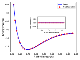
Figure 4: The ground state energy for the H₂ molecule as a function of internuclear distance R using the modified VQE based on the contex aware algorithm

VI Conclusion

In this paper, we have described a general storage method for matrices and shown circuits that execute quantum gates based on the data information. Since the gates are controlled by the data itself, this idea can be used for context aware quantum computing. We have also discussed how the circuit can be used with variational quantum eigensolver for any matrix related problems and for the simulation of molecular Hamiltonians. As an example, we have shown how the method can be used to calculate the ground state energy curve for the molecule H₂, which is in a complete agreement with the exact diagonalization results. Since any arbitrary real matrix can be decomposed into block diagonal matrices, this method may provide a new way to evolve quantum state by unitary/non-unitary operators through quantum circuits.

VII Acknowledgement

One of us, S.K would like to acknowledge the partial support from Purdue Integrative Data Science Initiative and the U.S. Department of Energy, Office of Basic Energy Sciences, under Award Number DE-SC0019215.

Appendix A Validation of the circuit in Fig.1

The controlled gate set in the circuit has the following matrix form:

$$\small\left(\begin{matrix}I^{\otimes 2n-2}\otimes X&&&\\ &I^{\otimes 2n-2}\otimes Z&&\\ &&\ddots&\\ &&&I^{\otimes 2n-2}\otimes I\end{matrix}\right)$$ (18)

We can represent the whole circuit more concisely by using the direct sum of matrices:

$$\small\left(H^{\otimes 3}\otimes I^{\otimes 2n-1}\right)\left(\bigoplus_{j=0}^{N/2}X\oplus\bigoplus_{j=0}^{N/2}Z\oplus\bigoplus_{j=0}^{N/2}-Z\oplus\dots\bigoplus_{j=0}^{N/2}I\right)$$ (19)

To illustrate the action of the circuit, we will use the example matrix $Q_{i}=Z\oplus XZ$ which leads to the following $\left|g_{ik}\right\rangle\left|k\right\rangle$s:

$$\left|g_{i0}\right\rangle\left|0\right\rangle=\left|\mathbf{1}\right\rangle\left|0\right\rangle\text{ and }\left|g_{i1}\right\rangle\left|1\right\rangle=\left|\mathbf{3}\right\rangle\left|1\right\rangle.$$ (20)

Then we form the following 6-qubit initial state:

$$\left|g_{i}\right\rangle\left|\psi\right\rangle=\frac{1}{\sqrt{2}}\left(\left|\mathbf{1}\right\rangle\left|0\right\rangle\left|\psi\right\rangle+\left|\mathbf{3}\right\rangle\left|1\right\rangle\left|\psi\right\rangle\right).$$ (21)

After applying the controlled gates ($CG$) to the initial state, we obtain:

$$\small CG\left|g_{i}\right\rangle\left|\psi\right\rangle=\frac{1}{\sqrt{2}}\left(\left|\mathbf{1}\right\rangle\left|0\right\rangle(Z\otimes Z)\left|\psi\right\rangle+\left|\mathbf{3}\right\rangle\left|1\right\rangle(XZ\otimes XZ)\left|\psi\right\rangle\right).$$ (22)

Applying the Hadamard gates to the first three qubits produces the following final state:

$$\small\begin{split}\frac{1}{4}\bigg{(}\big{(}\left|000\right\rangle-\left|001\right\rangle+\left|010\right\rangle-\left|011\right\rangle+\left|100\right\rangle-\left|101\right\rangle\\ +\left|110\right\rangle-\left|111\right\rangle\big{)}\left|0\right\rangle(Z\otimes Z)\left|\psi\right\rangle\\ +\big{(}\left|000\right\rangle-\left|001\right\rangle-\left|010\right\rangle+\left|011\right\rangle+\left|100\right\rangle-\left|101\right\rangle\\ -\left|110\right\rangle+\left|111\right\rangle\big{)}\left|1\right\rangle(XZ\otimes XZ)\left|\psi\right\rangle\bigg{)}.\end{split}$$ (23)

Here, the states where the first three qubits are in $\left|000\right\rangle$ includes the expected output which are:

$$\small\frac{1}{4}\big{(}\left|000\right\rangle\left|0\right\rangle(Z\otimes Z)\left|\psi\right\rangle+\left|000\right\rangle\left|1\right\rangle(XZ\otimes XZ)\left|\psi\right\rangle\big{)}.$$ (24)

The equivalent of $Q_{i}\left|\psi\right\rangle$ is produced on the amplitudes of the states:

$$\{\left|000000\right\rangle,\left|000001\right\rangle,\left|000110\right\rangle,\left|000111\right\rangle\}.$$ (25)

Appendix B Validations of the circuits in Fig.2 and Fig.3

In the circuit in Fig.2, we have the superpositioned input state $\left|g\right\rangle$. Before the Hadamard gates on the first register of the circuit, for different $\left|i\right\rangle$ on the output we have normalized $Q_{i}\left|\psi\right\rangle$ on the same states as given in (24) and (25). That means for $\left|\mathbf{0}\right\rangle$ on the first register we have normalized $Q_{0}\left|\psi\right\rangle$ on the chosen states, and for $\left|\mathbf{1}\right\rangle$ we have $Q_{1}\left|\psi\right\rangle$, and so on. By applying the Hadamard gates to the first register, for $\left|i\right\rangle=\left|\mathbf{0}\right\rangle$, we generate the normalized summation $\sum_{i}Q_{i}\left|\psi\right\rangle$ on the same chosen states.

Fig.3 is just the generalization of Fig.2 and acts the same way.

Appendix C A larger Hamiltonian divided into submatrices

$$\mathcal{H}=\left(\begin{matrix}H_{00}&H_{10}&H_{20}&H_{30}&H_{40}&H_{50}&H_{60}&H_{70}\\ H_{11}&H_{01}&H_{31}&H_{21}&H_{51}&H_{41}&H_{71}&H_{61}\\ H_{22}&H_{32}&H_{02}&H_{12}&H_{62}&H_{72}&H_{42}&H_{52}\\ H_{33}&H_{23}&H_{13}&H_{03}&H_{73}&H_{63}&H_{53}&H_{43}\\ H_{44}&H_{54}&H_{64}&H_{70}&H_{04}&H_{14}&H_{24}&H_{34}\\ H_{55}&H_{45}&H_{75}&H_{61}&H_{15}&H_{05}&H_{35}&H_{25}\\ H_{66}&H_{76}&H_{46}&H_{52}&H_{26}&H_{36}&H_{06}&H_{16}\\ H_{77}&H_{67}&H_{57}&H_{43}&H_{37}&H_{27}&H_{17}&H_{07}\\ \end{matrix}\right)_{16\times 16}.$$ (26)

References

- [1] Michael A Nielsen and Isaac L Chuang. Quantum Computation and Quantum Information. Cambridge University Press, 2010.
- [2] Andrew M Childs and Robin Kothari. Simulating sparse hamiltonians with star decompositions. In Conference on Quantum Computation, Communication, and Cryptography, pages 94–103. Springer, 2010.
- [3] Dominic W Berry, Andrew M Childs, Richard Cleve, Robin Kothari, and Rolando D Somma. Exponential improvement in precision for simulating sparse hamiltonians. In Forum of Mathematics, Sigma, volume 5. Cambridge University Press, 2017.
- [4] Ivan Kassal, James D Whitfield, Alejandro Perdomo-Ortiz, Man-Hong Yung, and Alán Aspuru-Guzik. Simulating chemistry using quantum computers. Annual review of physical chemistry, 62:185–207, 2011.
- [5] Jonathan Olson, Yudong Cao, Jonathan Romero, Peter Johnson, Pierre-Luc Dallaire-Demers, Nicolas Sawaya, Prineha Narang, Ian Kivlichan, Michael Wasielewski, and Alán Aspuru-Guzik. Quantum information and computation for chemistry. arXiv preprint arXiv:1706.05413, 2017.
- [6] S. Kais. Quantum Information and Computation for Chemistry: Advances in Chemical Physics, volume 154. Wiley Online Library, NJ, US., 2014.
- [7] Teng Bian, Daniel Murphy, Rongxin Xia, Ammar Daskin, and Sabre Kais. Quantum computing methods for electronic states of the water molecule. Molecular Physics, pages 1–14, 2019.
- [8] Rongxin Xia, Teng Bian, and Sabre Kais. Electronic structure calculations and the ising hamiltonian. The Journal of Physical Chemistry B, 122(13):3384–3395, 2017.
- [9] Rongxin Xia and Sabre Kais. Quantum machine learning for electronic structure calculations. Nature communications, 9(1):4195, 2018.
- [10] Alberto Peruzzo, Jarrod McClean, Peter Shadbolt, Man-Hong Yung, Xiao-Qi Zhou, Peter J Love, Alán Aspuru-Guzik, and Jeremy L O’brien. A variational eigenvalue solver on a photonic quantum processor. Nature communications, 5:4213, 2014.
- [11] Jarrod R McClean, Jonathan Romero, Ryan Babbush, and Alán Aspuru-Guzik. The theory of variational hybrid quantum-classical algorithms. New Journal of Physics, 18(2):023023, 2016.
- [12] Guang Hao Low and Isaac L Chuang. Optimal hamiltonian simulation by quantum signal processing. Physical review letters, 118(1):010501, 2017.
- [13] Anmer Daskin, Ananth Grama, Giorgos Kollias, and Sabre Kais. Universal programmable quantum circuit schemes to emulate an operator. The Journal of chemical physics, 137(23):234112, 2012.
- [14] Ammar Daskin and Sabre Kais. Direct application of the phase estimation algorithm to find the eigenvalues of the hamiltonians. Chemical Physics, 514:87–94, 2018.
- [15] Gregory D Abowd, Anind K Dey, Peter J Brown, Nigel Davies, Mark Smith, and Pete Steggles. Towards a better understanding of context and context-awareness. In International symposium on handheld and ubiquitous computing, pages 304–307. Springer, 1999.
- [16] Ammar Daskin and Sabre Kais. A generalized circuit for the hamiltonian dynamics through the truncated series. Quantum Information Processing, 17(12):328, Oct 2018.
- [17] PJJ O’malley, Ryan Babbush, Ian D Kivlichan, Jonathan Romero, Jarrod R McClean, Rami Barends, Julian Kelly, Pedram Roushan, Andrew Tranter, Nan Ding, et al. Scalable quantum simulation of molecular energies. Physical Review X, 6(3):031007, 2016.
- [18] Abhinav Kandala, Antonio Mezzacapo, Kristan Temme, Maika Takita, Markus Brink, Jerry M Chow, and Jay M Gambetta. Hardware-efficient variational quantum eigensolver for small molecules and quantum magnets. Nature, 549(7671):242, 2017.
- [19] Harry Buhrman, Richard Cleve, John Watrous, and Ronald De Wolf. Quantum fingerprinting. Physical Review Letters, 87(16):167902, 2001.
- [20] Jarrod R McClean, Ian D Kivlichan, Kevin J Sung, Damian S Steiger, Yudong Cao, Chengyu Dai, E Schuyler Fried, Craig Gidney, Brendan Gimby, Pranav Gokhale, et al. Openfermion: the electronic structure package for quantum computers. arXiv preprint arXiv:1710.07629, 2017.