Fence GAN: Towards Better Anomaly Detection

Abstract

Anomaly detection is a classical problem where the aim is to detect anomalous data that do not belong to the normal data distribution. Current state-of-the-art methods for anomaly detection on complex high-dimensional data are based on the generative adversarial network (GAN). However, the traditional GAN loss is not directly aligned with the anomaly detection objective: it encourages the distribution of the generated samples to overlap with the real data and so the resulting discriminator has been found to be ineffective as an anomaly detector. In this paper, we propose simple modifications to the GAN loss such that the generated samples lie at the boundary of the real data distribution. With our modified GAN loss, our anomaly detection method, called Fence GAN (FGAN), directly uses the discriminator score as an anomaly threshold. Our experimental results using the MNIST, CIFAR10 and KDD99 datasets show that Fence GAN yields the best anomaly classification accuracy compared to state-of-the-art methods.

1 Introduction

Anomaly detection is a well-known problem in artificial intelligence where one aims to identify anomalous instances that do not belong to the normal data distribution [5, 14]. It is used in a wide range of applications such as network intrusion [10], credit card fraud [29], crowd surveillance [20, 23], healthcare [25] and many more. Traditional classifiers trained in a supervised setting do not work well in anomaly detection since the anomalous data is usually unavailable or very few. Hence, anomaly detectors are usually trained in an unsupervised setting where the distribution of the normal data is learned and instances that are unlikely to be under this distribution are identified as anomalous.

For complex high-dimensional datasets such as images, traditional methods for anomaly detection are unsuitable. Instead, recent methods based on generative adversarial networks (GANs) have shown state-of-the-art anomaly detection performance by exploiting GANs ability to model high-dimensional data distributions. However, we identify a shortcoming of current GAN-based anomaly detection methods: the usual GAN objective encourages the distribution of generated samples to overlap with the real data, and this is not directly aligned with the anomaly detection objective. The resulting discriminator has been found to be ineffective in detecting anomalous data. Hence, in this paper, we propose a simple modification to the GAN objective such that the generated samples lie at the boundary of real data distribution instead of overlapping it. Our method, which we call Fence GAN (FGAN), trains in the usual adversarial manner with the modified objective and we show that the resulting discriminator can be used as an anomaly detector. We conducted experiments on MNIST, CIFAR10 and KDD99 datasets and show that FGAN outperforms state-of-the-art methods at anomaly detection.

The main contributions of this paper are as follows:

• We propose an anomaly detection method using the basic GAN architecture and framework.

• We modify the GAN loss such that the samples are generated only at the boundary of the data distribution unlike the traditional GANs that generate samples over the whole data distribution.

• The proposed method is tested on MNIST, CIFAR10 and KDD99 datasets, showing improved accuracies over other state-of-the-art methods.

2 Related work

Traditional methods for anomaly detection include one-class SVM [26], nearest neighbor [9], clustering [28], kernel density estimation [21] and hidden markov models [13]. However, such methods are not suitable for high-dimensional image data. Recent developments in deep learning have led to significant progress in supervised learning tasks on complex image datasets [15, 24]. For anomaly detection, deep learning based methods include deep belief networks [8], variational autoencoders [2, 30] and adversarial autoencoders [34, 18, 4, 19].

Among the deep learning methods, generative adversarial networks (GANs) [11, 22] have been the subject of extensive research as they show state-of-the-art performance in modeling complex high-dimensional image distributions. Similarly, GANs have been used for anomaly detection. In AnoGAN [25], the authors propose an anomaly detector where the GAN is first trained on the normal images, and for a test image, the latent space is iteratively searched to find the latent vector that best reconstructs the test image. The anomaly score is a combination of the reconstruction loss and the loss between the intermediate discriminator feature of the test image and the reconstructed image. A similar framework is used in ADGAN [7], where the anomaly score is based only on reconstruction loss, the search in latent space is repeated with multiple seeds and both the latent vector and generator are optimized. A more recent method, called Efficient GAN [32], makes use of the BiGAN model that is able to map from the image to latent space without iterative search, resulting in superior anomaly detection performance and faster test times. Finally, in the GANomaly framework [1], the generator consists of encoder-decoder-encoder subnetworks and the anomaly score is based on a combination of encoding, reconstruction and feature matching losses. GANomaly has shown superior performance compared to AnoGAN and Efficient GAN on several image datasets such as MNIST and CIFAR10.

Except for GANomaly, the GAN-based anomaly detection methods above train GAN with the usual minimax loss function where the generator aims to generate samples that overlap with the data distribution. Under the usual GAN loss function, the discriminator probability score was found to be ineffective [7], and we hypothesize that this is because the discriminator is not explicitly trained to fence the boundary of the data distribution. Contrary to these methods, our proposed Fence GAN aims to learn the boundary of the normal data distribution. We achieve this by modifying the generator’s objective to aim to generate data lying on the boundary of the normal data distribution, instead of overlapping with the data distribution. At test time, the anomaly score is simply the discriminator score given to the input data. Our alternative generator objective is similar to the one in Dai et al. [6], where they show that for the discriminator to be a good classifier, the generator has to produce complement samples instead of matching with the true data distribution. With the modified GAN loss, Fence GAN does not need to rely on reconstruction loss from the generator and does not require modifications to the basic GAN architecture unlike Efficient GAN and GANomaly.

3 Method

3.1 Original GAN loss function

In the original generative adversarial network by Goodfellow et al. [12], for a set $\mathcal{X}$ of $N$ number of data points $\mathcal{X}=\{\boldsymbol{x}_{1},\boldsymbol{x}_{2},...,\boldsymbol{x}_{N}\}$ with $\boldsymbol{x}_{i}$ in a Euclidean data space $\mathbb{R}^{d},\>d\in\mathbb{Z}^{+}$, $i=1,2,..,N$, which is sampled from a data distribution $p_{data}:\mathbb{R}^{d}\rightarrow\mathbb{R}^{+}$, we seek to map points from a prior noise distribution $p_{noise}:\mathbb{R}^{k}\rightarrow\mathbb{R}^{+},\>k\in\mathbb{Z}^{+}$ to $p_{data}$. For example, if each data point represents an image, then $d$ would be the number of pixels in the image. The dimension $k$ is set arbitrarily.

The mapping from $p_{noise}$ to $p_{data}$ is done by first using a differentiable function, represented by a “generator” multilayer perceptron $G_{\theta}$ with $\theta$ being its weights and biases, to map $p_{noise}$ to the generated distribution $p_{g}:\mathbb{R}^{d}\rightarrow\mathbb{R}^{+}$ from the output $G_{\theta}(\boldsymbol{z}),G_{\theta}(\boldsymbol{z})\in\mathbb{R}^{d}$ of $G_{\theta}$ and $\boldsymbol{z}$ is drawn from $p_{noise}$. In addition, we also have a “discriminator” multilayer perceptron $D_{\phi}$ with $\phi$ being its weights and biases, which outputs a real value $D_{\phi}(\boldsymbol{x})\in[0,1]$ that represents the probability of $\boldsymbol{x}$ - a point in $\mathbb{R}^{d}$ being drawn from $p_{data}$ rather than from $p_{g}$. $D_{\phi}$ and $G_{\theta}$ engage in a two-player minimax game, with $D_{\phi}$ and $G_{\theta}$ being alternatingly trained to minimize their respective loss functions as follows:

$$\mathcal{L}_{G_{\theta}}^{GAN}(G_{\theta},D_{\phi},\mathcal{Z}) =\frac{1}{N}\sum_{i=1}^{N}\Bigg{[}\log(1-D_{\phi}(G_{\theta}(\boldsymbol{z}_{i})))\Bigg{]}$$ (1)

$$\mathcal{L}_{D_{\phi}}^{GAN}(G_{\theta},D_{\phi},\mathcal{X},\mathcal{Z}) =\frac{1}{N}\sum_{i=1}^{N}\Bigg{[}-\log(D_{\phi}(\boldsymbol{x}_{i}))-\log(1-D_{\phi}(G_{\theta}(\boldsymbol{z}_{i})))\Bigg{]}$$ (2)

where $\mathcal{Z}=\{\boldsymbol{z}_{1},\boldsymbol{z}_{2},...,\boldsymbol{z}_{N}\}$ is sampled from $p_{noise}$. $\mathcal{L}_{G_{\theta}}^{GAN}$ is the loss function of $G_{\theta}$ and $\mathcal{L}_{D_{\phi}}^{GAN}$ is the loss function of $D_{\phi}$.

In this way, $D_{\phi}$ is trained to differentiate whether $\boldsymbol{x}$ is drawn from $p_{data}$ or from $p_{g}$. Meanwhile, $G_{\theta}$ is trained to map $p_{noise}$ to $p_{g}$ so as to maximise the score of its generated points as given by the discriminator, that is, $D_{\phi}(G_{\theta}(\boldsymbol{z}))$.

The training of GAN is completed if the distribution $p_{g}$ is indistinguishable from $p_{data}$. When this occurs, $p_{data}$ is estimated by $p_{g}$. Therefore, the mapping of points from $p_{noise}$ to $p_{g}$, which is represented by $G_{\theta}$, is also the mapping of points from $p_{noise}$ to $p_{data}$.

3.2 Modified loss functions

We propose Fence GAN (FGAN) which has a different objective from the original GAN’s. Whereas the original GAN aims to generate $p_{g}=p_{data}$, that is, to generate points at regions of high data density, our objective is to generate points around the boundary of $\mathcal{X}$, which we denote as $\delta\mathcal{X}$. This will enable our discriminator, at the end of training, to draw a boundary “tightly” around $\mathcal{X}$. Such a discriminator can then be used as a one-class classifier or an anomaly detector.

Learning $\delta\mathcal{X}$ directly is known to be an extremely difficult problem in high dimensions [27]. Thus, we use the discriminator score to define the domain of $\delta\mathcal{X}$ and then estimate $\delta\mathcal{X}$ using the generator in FGAN. The generated points $G_{\theta}(\boldsymbol{z})$ then must enclose the real data points tightly as shown in Figure 1(A). In order to achieve our objective, we propose a series of modifications to the loss functions for the generator and discriminator: encirclement and dispersion losses for generator, and weighted discriminator loss for discriminator.

3.2.1 Generator

Encirclement Loss

In our proposed FGAN, we want the generator to generate points $G_{\theta}(\boldsymbol{z})$ that lie in $\delta\mathcal{X}$. We first define points on $\delta\mathcal{X}$ to be those that yield a discriminator score of $\alpha$. To reflect this, the objective function of the generator in FGAN to be minimized is therefore:

$$EL\big{(}G_{\theta},D_{\phi},\mathcal{Z}\big{)} =\frac{1}{N}\sum_{i=1}^{N}\Bigg{[}\log(\lvert\alpha-D_{\phi}(G_{\theta}(\boldsymbol{z}_{i}))\rvert)\Bigg{]}$$ (3)

where $\alpha\in(0,1)$ is used for the generator to generate points on $\delta\mathcal{X}$. The rationale for Eq. (3) is that points generated inside of $\mathcal{X}$ will have a discriminator score higher than $\alpha$ and hence the generator will be penalised. On the other hand, points generated far from $\mathcal{X}$ will have a discriminator score less than $\alpha$ and hence the generator is also penalised. Only when points are generated at the $\alpha$-level set of the discriminator score will they yield optimal generator loss. This level set should ideally tightly enclose the real data points. In our experiments, we tune the value for $\alpha$ as a hyperparameter.

Dispersion loss

Based on the encirclement loss alone, however, there is no guarantee that the generated points will cover the entirety of $\delta\mathcal{X}$, it may only cover a small part of it, as shown in Figure 1(C). We note that this is similar to the mode collapse problem in GAN. The dispersion loss, which maximizes distance of the generated data points from their centre of mass $\boldsymbol{\mu}$, $\boldsymbol{\mu}\in\mathbb{R}^{d}$, is thus introduced to encourage the generated points to cover the whole boundary.

$$\boldsymbol{\mu}=(\mu_{1},\mu_{2},...,\mu_{d})$$

$$\boldsymbol{\mu}=\frac{1}{N}\sum_{i=1}^{N}G_{\theta}(\boldsymbol{z}_{i})$$

The dispersion loss is thus:

$$\ DL(G_{\theta},\mathcal{Z})=\frac{1}{\frac{1}{N}{\sum_{i=1}^{N}(\left\lVert G_{\theta}(\boldsymbol{z}_{i})-\boldsymbol{\mu}\right\rVert_{2})}}$$ (4)

We use $L2$ distance because in our experiments we found that it works better compared to $L1$ and $L\infty$ distances. The loss function of the generator in FGAN to be minimized is defined as the weighted sum of the encirclement loss and the dispersion loss:

$$\mathcal{L}_{generator}^{FGAN}\big{(}G_{\theta},D_{\phi},\mathcal{Z}\big{)} =EL\>+\beta\times\>DL$$

$$=\frac{1}{N}\sum_{i=1}^{N}\Bigg{[}\log\Big{[}\lvert\alpha-D_{\phi}(G_{\theta}(\boldsymbol{z}_{i}))\rvert\Big{]}\Bigg{]}+\beta\times\frac{1}{\frac{1}{N}{\sum_{i=1}^{N}(\left\lVert G_{\theta}(\boldsymbol{z}_{i})-\boldsymbol{\mu}\right\rVert_{2})}}$$ (5)

where $\beta$ is the dispersion hyperparameter with $\beta\in\mathbb{R}^{+}$.

3.2.2 Discriminator

Weighted Discriminator Loss

As the generator becomes better in approximating $\delta\mathcal{X}$, the discriminator faces a trade-off: to classify real data correctly or classify generated data correctly. If the discriminator focuses more on classifying generated data correctly, then the discriminator will start to classify real data as generated data. Thus, the loss function of the discriminator should be modified to prioritise classifying real data correctly:

$$\mathcal{L}_{discriminator}^{FGAN}\big{(}G_{\theta},D_{\phi},\mathcal{X},\mathcal{Z}\big{)} =\frac{1}{N}\sum_{i=1}^{N}\Bigg{[}-\log\big{(}D_{\phi}(\boldsymbol{x}_{i})\big{)}-\gamma\log\bigg{(}1-D_{\phi}(G_{\theta}(\boldsymbol{z}_{i})\big{)}\bigg{)}\Bigg{]}$$ (6)

where $\gamma$ is the anomaly hyperparameter with $\gamma\in(0,1]$. When $\gamma$ is less than 1, the discriminator will focus more on classifying the real data points correctly, thus its decision boundary is less likely to bend into the domain of $\mathcal{X}$, allowing the generator to better estimate $\delta\mathcal{X}$. We empirically tune $\gamma$ for each dataset.

3.3 Fence GAN (FGAN)

FGAN is composed of a generator and a discriminator being trained one after another like a typical GAN. The number of steps to train $G_{\theta}$ and $D_{\phi}$ for each iteration are hyperparameters to be tuned. However for simplicity, we train both networks once in each iteration.

Algorithm 1 Stochastic gradient descent training of FGAN.

for number of training iterations do

     $\bullet$ Sample noise samples $\mathcal{Z}=\{\boldsymbol{z}_{1},\boldsymbol{z}_{2},...,\boldsymbol{z}_{N}\}$ from prior $p_{noise}$

     $\bullet$ Update the generator’s parameters:

$$\theta\leftarrow\theta-\eta_{g}\nabla_{\theta}\mathcal{L}_{generator}^{FGAN}\big{(}G_{\theta},D_{\phi},\mathcal{Z}\big{)}$$

     $\bullet$ Resample noise samples $\mathcal{Z}=\{\boldsymbol{z}_{1},\boldsymbol{z}_{2},...,\boldsymbol{z}_{N}\}$ from prior $p_{noise}$

     $\bullet$ Sample data samples $\mathcal{X}=\{\boldsymbol{x}_{1},\boldsymbol{x}_{2},...,\boldsymbol{x}_{N}\}$ from real data distribution $p_{data}$

     $\bullet$ Update the discriminator’s parameters:

$$\phi\leftarrow\phi-\eta_{d}\nabla_{\phi}\mathcal{L}_{discriminator}^{FGAN}\big{(}G_{\theta},D_{\phi},\mathcal{Z},\mathcal{X}\big{)}$$

end for

The generator and discriminator learning rates $\eta_{g}$ and $\eta_{d}$ are to be set.

4 Experiments

In our experiments, we tested FGAN on a synthetic 2D dataset to study the training process in FGAN. Next, we tested FGAN for anomaly detection on three datasets: MNIST, CIFAR10 and KDD99, comparing the performance to state-of-the-art anomaly detection methods.

4.1 2D synthetic dataset

We illustrate the effect of FGAN using a 2D synthetic dataset where the data is sampled from a unimodal normal distribution, as shown in Figure 1. The red points represent the real data while the blue points are the generated points. The color of the shaded background represents the discriminator score, where the score increases from blue to red. We trained 5 different FGAN models with different hyperparameters over 30,000 epochs.

In (A), we show snapshots of training process at 4 epochs for an FGAN trained with optimal hyperparameters, yielding a good discriminator at the end of the training. The other examples show hyperparameters that lead to suboptimal performance. (B) shows the result of original GAN [12], where the real data points and generated data points are indistinguishable and the discriminator decision boundary does not surround the real data. (C) illustrates an example of generated points coalescing in one small region and the discriminator classifies most of the data space as positive instances. (D) shows an example of loosely enclosed generated points where the discriminator decision boundary is away from the real data points. (E) shows another example of indistinguishable real data and generated data distributions with bad discriminator decision boundaries. This experiment on the 2D dataset shows that under the optimal hyperparameters, the encirclement loss, dispersion loss and weighted discriminator loss in FGAN give rise to the desired result of the generated samples forming a tight boundary around the dataset.

Figure 1: FGAN on a normal distribution in two dimensions. Red points are data points and blue points are generated points. The color of the shaded background represents the discriminator score. We trained 5 different models with different hyperparameters over $3\times 10^{4}$ epochs. (A) shows snapshots of training process for a FGAN trained with optimal hyperparameters, yielding a good discriminator in the end of the training. (B)-(E) are examples of hyperparameters that lead to suboptimal performance of FGAN.

4.2 MNIST

To show the effectiveness of our proposed idea, we run FGAN for anomaly detection on the MNIST dataset [17]. In each case, we consider data points from a class as ‘anomalous’ (positive class) and data points from the other 9 classes as ‘normal’ (negative class). We then split the entire MNIST dataset which consists of 70000 images from 10 classes into 2 sets as follows: Training set consists of 80% of all data points in the ‘normal’ class. Testing set consists of the rest 20% of data in the ‘normal’ class and all data in the ‘anomalous’ class. We then evaluate our model as a binary classifier for normal and anomalous data. Our performance is measured by Area Under Precision and Recall Curve (AUPRC). The architecture as well as hyperparameters to train FGAN are presented in Table 1.

Operation	Kernel	Strides	Features Maps/Units	BN?	Activation
Generator
Dense			1024	✓	ReLU
Dense			7$\times$7$\times$128	✓	ReLU
Transposed Convolution	4$\times$4	2$\times$2	64	✓	ReLU
Transposed Convolution	4$\times$4	2$\times$2	1	$\times$	Tanh
Latent Dimension	200
Encirclement $\alpha$	0.1
Dispersion $\beta$	30
Optimizer	Adam(lr=2e-5, decay=1e-4)
Discriminator
Convolution	4$\times$4	2$\times$2	64	$\times$	Leaky ReLU
Convolution	4$\times$4	2$\times$2	64	$\times$	Leaky ReLU
Dense			1024	$\times$	Leaky ReLU
Dense			1	$\times$	Sigmoid
Leaky ReLU slope	0.1
Optimizer	Adam(lr=1e-5, decay=1e-4)
Anomaly $\gamma$	0.1
Epochs	100
Batchsize	200

Table 1: Architecture and hyperparameters of FGAN on MNIST Dataset

We train FGAN for 100 epochs with a training batch size of 100 and obtain the average AUPRC across 3 different seeds for each anomalous class. Mean AUPRC in comparison to other benchmark methods are shown in Figure 2. The other benchmark methods are trained using the same setup for splitting of the train and test sets. We reimplement GANomaly [1] using the hyperparameters used by the authors to obtain the AUPRC while the results for EGBAD, AnoGAN and VAE were taken from [31]. As seen from the AUPRC figures, FGAN has the highest accuracy for all but one digit class. Interestingly, for digit classes where the other methods perform badly (eg. digits 1, 7, 9), FGAN’s detection accuracy remains high. This shows FGAN’s robustness in anomaly detection for the MNIST dataset.

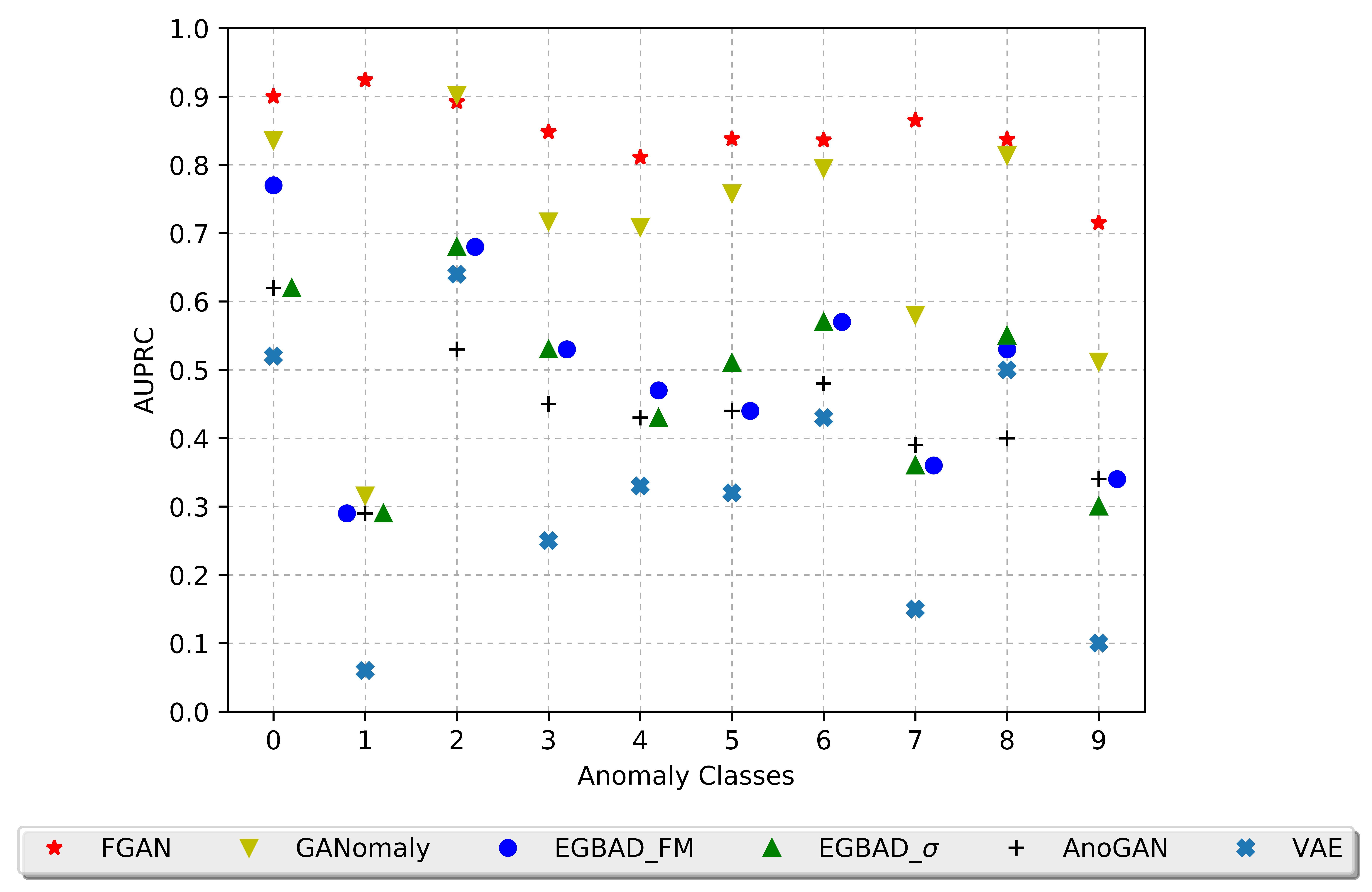
Figure 2: Detection accuracies for FGAN and benchmark methods on MNIST dataset.

4.3 CIFAR10

Next, we run the anomaly detection test on the CIFAR10 dataset [16]. Similar to the MNIST experiment, we consider data points from a class as ‘anomalous’ and data points from the other 9 classes as ‘normal’. We split the entire CIFAR10 dataset with 60000 images into a training set consisting of 80% of images in the ‘normal’ class and a testing set consisting of the rest 20% of data in the ‘normal’ class and all data in the ‘anomalous’ class. We train FGAN for 150 epochs with a training batch size of 128. The performance is measured by the Area Under Receiver Operating Characteristics (AUROC) curve, averaged over 3 seeds. The network architecture and hyperparameters to train FGAN are presented in Table 2.

Operation	Kernel	Strides	Feature Maps / Units	BN?	Activation
Generator
Dense			2$\times$2$\times$256	$\checkmark$	Leaky ReLU
Transposed Convolution	5$\times$5	2$\times$2	128	$\checkmark$	Leaky ReLU
Transposed Convolution	5$\times$5	2$\times$2	64	$\checkmark$	Leaky ReLU
Transposed Convolution	5$\times$5	2$\times$2	32	$\checkmark$	Leaky ReLU
Transposed Convolution	5$\times$5	2$\times$2	3	$\times$	Tanh
Latent Dimension	256
Leaky ReLU Slope	0.2
Encirclement $\alpha$	0.5
Dispersion $\beta$	10
Optimizer	Adam(lr=1e-3, beta_1 = 0.5, beta_2 = 0.999, decay=1e-5)
Discriminator
Convolution	5$\times$5	2$\times$2	32	$\checkmark$	Leaky ReLU
Convolution	5$\times$5	2$\times$2	64	$\checkmark$	Leaky ReLU
Convolution	5$\times$5	2$\times$2	128	$\checkmark$	Leaky ReLU
Convolution	5$\times$5	2$\times$2	256	$\times$	Leaky ReLU
Dropout			0.2	$\times$
Dense			1	$\times$	Sigmoid
Leaky ReLU Slope	0.2
Weight Decay	0.5
Optimizer	Adam(lr=1e-4, beta_1 = 0.5, beta_2 = 0.999, decay=1e-5)
Anomaly $\gamma$	0.5
Epochs	150
Batch Size	128

Table 2: Architecture and hyperparameters of FGAN on CIFAR-10 Dataset

The anomaly detection results are shown in Figure 3. For all but one anomaly class, FGAN’s accuracy is the highest among all methods, with AUROC of at least 60% across all classes. For the challenging ‘bird’ class where the state-of-the-art GANomaly method has an AUROC of just above 50%, FGAN manages an AUROC of 60%, showing its detection robustness.

In Figure 4, we analyze the distribution of discriminator scores for the normal test images, anomalous images and generated images where the anomalous class is ‘ship’. The normal test images scores are skewed towards the high score of 1.0 which is expected from the FGAN loss function. The anomalous images scores show a bimodal distribution with modes at 0.3 and 1.0, which means some anomalous images are challenging to detect. This explains the relatively good anomaly detection results in Figure 3. The distribution of scores for generated images is spread across the entire range which means the generated samples do not converge at a score of $\alpha=0.5$, although this has not significantly impacted anomaly detection performance.

Table 3 shows the average discriminator score for the anomalous ‘ship’ class, the other 9 classes and the generated images. All scores are taken from the test set. Interestingly the ‘airplane’ class has a lower score than the anomalous ‘ship’ class, and this may indicate that these two classes are semantically similar and challenging to differentiate compared to other classes. In Figure 5, we show examples of the generated images with their corresponding discriminator scores. The generated images are relatively realistic, resembling natural images, though there is no identifiable pattern from the discriminator scores.

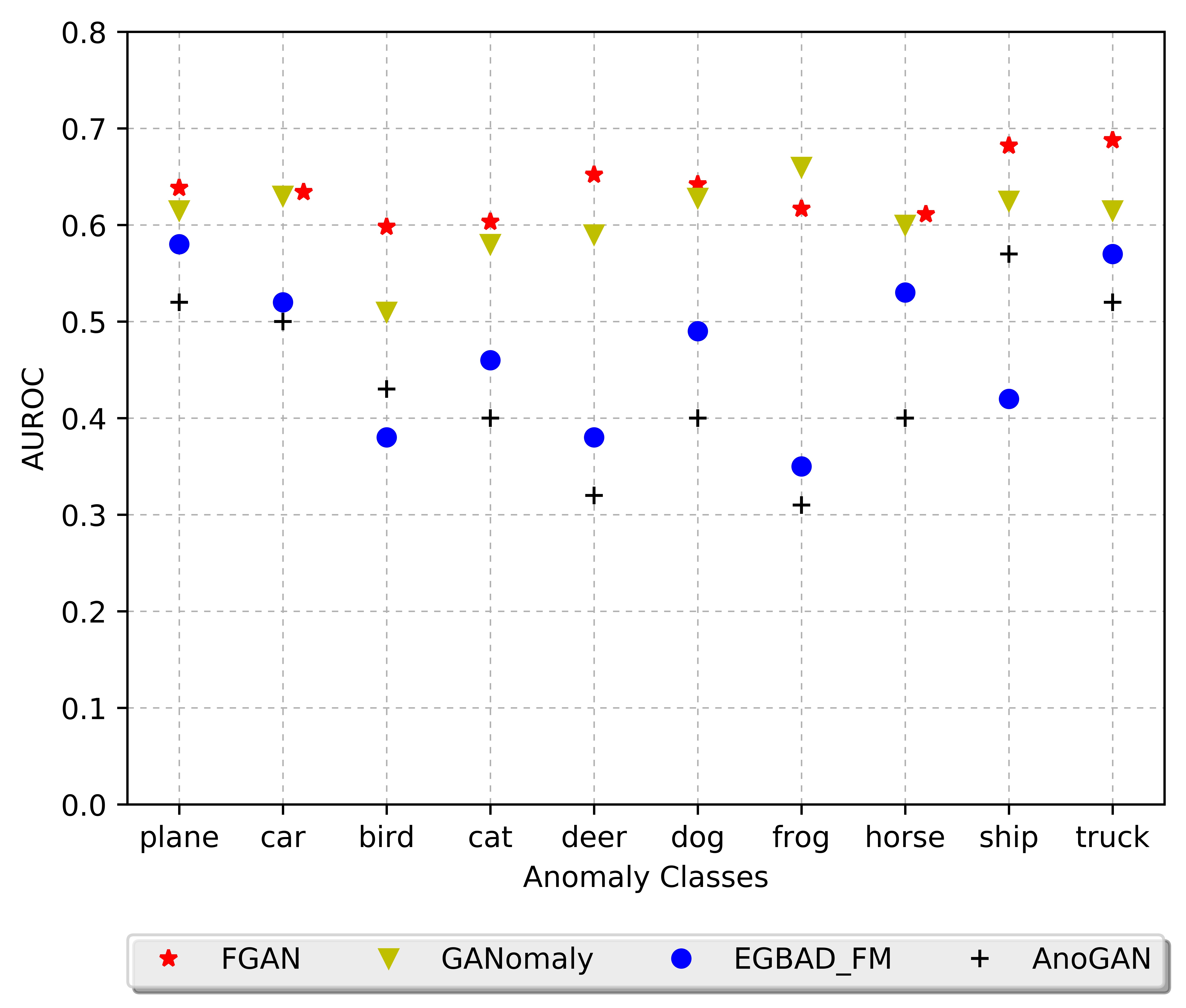
Figure 3: Detection accuracies for FGAN and benchmark methods on the CIFAR10 dataset.

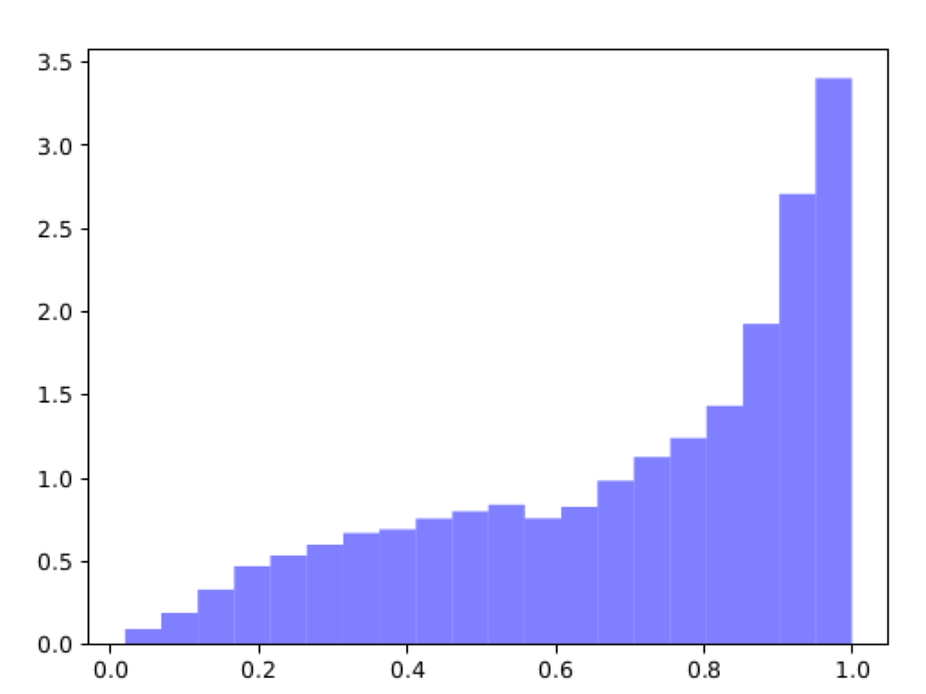
(a) Normal test images

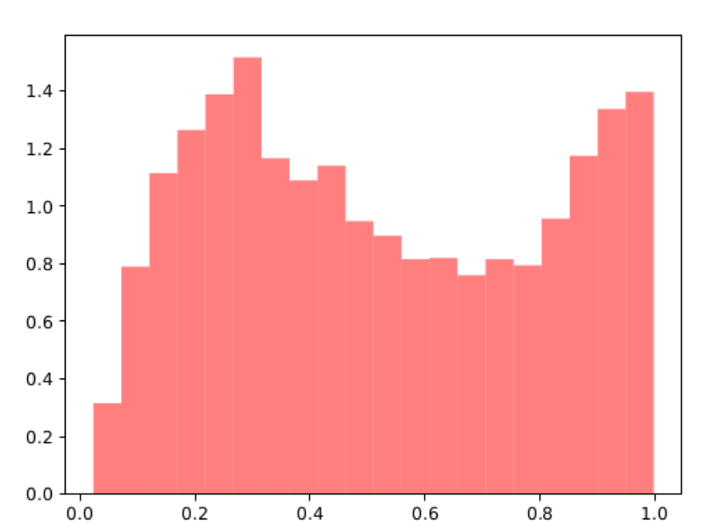
(b) Anomalous images

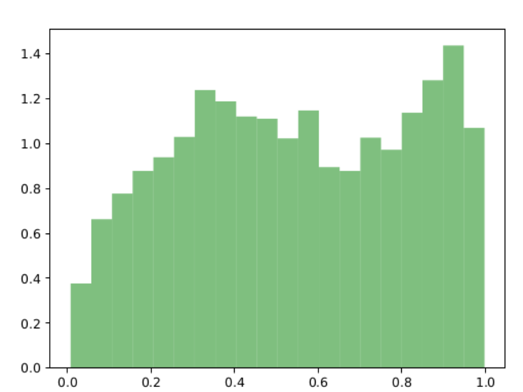
(c) Generated images

Figure 4: CIFAR10 anomalous class: ship. Histogram of discriminator scores for (a) normal test images, (b) anomalous images and (c) generated images. The normal test images have a distribution that is skewed towards higher scores, which is expected from the FGAN loss function. The distributions for the anomalous and generated images are bimodal.

Class	Airplane	Ship	Generated images	Dog	Bird	Cat	Car	Truck	Deer	Horse	Frog
Average score	0.505	0.521	0.543	0.669	0.671	0.686	0.717	0.737	0.75	0.752	0.795

Table 3: CIFAR10 anomalous class: ship. Average discriminator scores for the anomalous ‘ship’ class, the other 9 classes and the generated images. All scores were taken from the test set and the average scores are shown in increasing order.

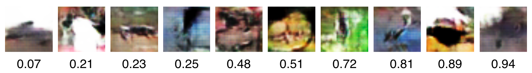
Figure 5: CIFAR10 anomalous class: ship. Examples of generated images shown in increasing order of the discriminator score.

4.4 KDD99

In order to further validate the merits of our approach, we test FGAN on the KDDCUP99 10 percent dataset [3]. We follow the experimental setup of [35] [31] in our experiments. In the KDD99 dataset, data is stratified into the ‘non-attack’ class and other classes with various attacks. We lump all the other classes with various attacks as one class and call it the ‘attack’ class. We then train FGAN on the ‘attack’ class only because the proportion of data belonging to the ‘attack’ class is much larger than the proportion of data belonging to the ‘non-attack’ class. The objective is to detect the ‘non-attack’ instances.

We split the KDD99 dataset as follows: Training set consists of 50% of all data points in the ‘attack’ class. Testing set consists of the remaining 50% of data in the ‘attack’ class and 50% of data in the ‘non-attack’ class. We then evaluate our approach against Efficient-GAN. The architecture and hyperparameters to train FGAN for KDD99 dataset is shown in Table 4.

Operation	Units	Non Linearity	Dropout	L2 Regularization
Generator			0	0
Dense	64	ReLU	0.2	0
Dense	128	ReLU	0.2	0
Dense (output)	121	Linear	0	0
Latent Dimension	32
Encirclement $\alpha$	0.5
Dispersion $\beta$	30
Optimizer	Adam(lr = 1e-4, decay = 1e-3)
Discriminator			0
Dense	256	Leaky ReLU	0	0
Dense	128	Leaky ReLU	0	0
Dense	128	Leaky ReLU	0	0
Dense (output)	1	Sigmoid	0
Leaky ReLU Slope	0.1
Optimizer	SGD(lr = 8e-6, decay = 1e-3)
Anomaly $\gamma$	0.5

Table 4: Architecture and hyperparameters for FGAN on KDD99 Dataset.

We train with a batch size of 256 for both discriminator and generator for 50 epochs. The precision, recall and F1 scores are averaged over 10 different consecutive seeds, as shown in Table 5. FGAN has the best anomaly detection accuracies compared to the other benchmark methods.

Model	Precision	Recall	F1
OC-SVM	0.7457	0.8523	0.7954
DSEBM-r	0.8521	0.6472	0.7328
DSEBM-e	0.8619	0.6446	0.7399
DAGMM-NVI	0.9290	0.9447	0.9368
DAGMM	0.9297	0.9442	0.9369
AnoGANfm	$0.88\pm 3\times 10^{-2}$	$0.83\pm 3\times 10^{-2}$	$0.89\pm 3\times 10^{-2}$
AnoGANsigmoid	$0.8\pm 0.1$	$0.8\pm 0.1$	$0.8\pm 0.1$
Efficient-GANfm	$0.9\pm 0.1$	$0.95\pm 2\times 10^{-2}$	$0.91\pm 7\times 10^{-2}$
Efficient-GANsigmoid	$0.92\pm 7\times 10^{-2}$	$0.96\pm 1\times 10^{-2}$	$0.94\pm 4\times 10^{-2}$
FGAN	0.954$\pm 9\times 10^{-3}$	0.969$\pm 9\times 10^{-3}$	0.95$\pm 2\times 10^{-2}$

Table 5: Performance on the KDD99 dataset. Values for OC-SVM, DSEBM, DAGMM were obtained from [33], [35]. Values for AnoGAN and Efficient-GAN were obtained from [31]. Precision, Recall, and F1 Score are calculated with ‘non-attack’ class being the positive class and ‘attack’ class being the negative class.

5 Discussion

State-of-the-art anomaly detection methods for complex high-dimensional data are based on generative adversarial networks. However, in this paper, we identify that the usual GAN loss objective is not directly aligned with the anomaly detection objective: the loss encourages the distribution of generated samples to overlap with real data. Hence, the resulting discriminator has been found to be ineffective for anomaly detector. Hence, we propose simple modifications to the GAN loss such that the generated samples lie at the boundary of real data distribution. Our method, called Fence GAN, uses the discriminator score as anomaly score. With the modified GAN loss, Fence GAN does not need to rely on reconstruction loss from the generator and does not require modifications to the basic GAN architecture unlike Efficient GAN and GANomaly.

On the MNIST, CIFAR10 and KDD99 datasets, Fence GAN outperforms existing methods in anomaly detection. We have shown that with simple modifications to the GAN loss, the basic GAN architecture and training scheme can produce an effective anomaly detector for complex high-dimensional data.

References

- Akcay et al. [2018] Samet Akcay, Amir Atapour-Abarghouei, and Toby P Breckon. Ganomaly: Semi-supervised anomaly detection via adversarial training. arXiv preprint arXiv:1805.06725, 2018.
- An and Cho [2015] Jinwon An and Sungzoon Cho. Variational autoencoder based anomaly detection using reconstruction probability. Special Lecture on IE, 2:1–18, 2015.
- Bay et al. [2000] Stephen D Bay, Dennis F Kibler, Michael J Pazzani, and Padhraic Smyth. The uci kdd archive of large data sets for data mining research and experimentation. SIGKDD Explorations, 2:81, 2000.
- Beggel et al. [2019] Laura Beggel, Michael Pfeiffer, and Bernd Bischl. Robust anomaly detection in images using adversarial autoencoders. arXiv preprint arXiv:1901.06355, 2019.
- Chandola et al. [2009] Varun Chandola, Arindam Banerjee, and Vipin Kumar. Anomaly detection: A survey. ACM computing surveys (CSUR), 41(3):15, 2009.
- Dai et al. [2017] Zihang Dai, Zhilin Yang, Fan Yang, William W Cohen, and Ruslan R Salakhutdinov. Good semi-supervised learning that requires a bad gan. In Advances in Neural Information Processing Systems, pages 6510–6520, 2017.
- Deecke et al. [2018] Lucas Deecke, Robert Vandermeulen, Lukas Ruff, Stephan Mandt, and Marius Kloft. Anomaly detection with generative adversarial networks. 2018.
- Erfani et al. [2016] Sarah M Erfani, Sutharshan Rajasegarar, Shanika Karunasekera, and Christopher Leckie. High-dimensional and large-scale anomaly detection using a linear one-class svm with deep learning. Pattern Recognition, 58:121–134, 2016.
- Eskin et al. [2002] Eleazar Eskin, Andrew Arnold, Michael Prerau, Leonid Portnoy, and Sal Stolfo. A geometric framework for unsupervised anomaly detection. In Applications of data mining in computer security, pages 77–101. Springer, 2002.
- Garcia-Teodoro et al. [2009] Pedro Garcia-Teodoro, Jesus Diaz-Verdejo, Gabriel Maciá-Fernández, and Enrique Vázquez. Anomaly-based network intrusion detection: Techniques, systems and challenges. computers & security, 28(1-2):18–28, 2009.
- Goodfellow et al. [2014a] Ian Goodfellow, Jean Pouget-Abadie, Mehdi Mirza, Bing Xu, David Warde-Farley, Sherjil Ozair, Aaron Courville, and Yoshua Bengio. Generative adversarial nets. In Advances in neural information processing systems, pages 2672–2680, 2014a.
- Goodfellow et al. [2014b] Ian J. Goodfellow, Jean Pouget-Abadie, Mehdi Mirza, Bing Xu, David Warde-Farley, Sherjil Ozair, Aaron C. Courville, and Yoshua Bengio. Generative adversarial nets. In NIPS, 2014b.
- Görnitz et al. [2015] Nico Görnitz, Mikio Braun, and Marius Kloft. Hidden markov anomaly detection. In International Conference on Machine Learning, pages 1833–1842, 2015.
- Hawkins [1980] Douglas M Hawkins. Identification of outliers, volume 11. Springer, 1980.
- He et al. [2016] Kaiming He, Xiangyu Zhang, Shaoqing Ren, and Jian Sun. Deep residual learning for image recognition. In Proceedings of the IEEE conference on computer vision and pattern recognition, pages 770–778, 2016.
- Krizhevsky and Hinton [2009] Alex Krizhevsky and Geoffrey Hinton. Learning multiple layers of features from tiny images. Technical report, Citeseer, 2009.
- LeCun and Cortes [2010] Yann LeCun and Corinna Cortes. MNIST handwritten digit database. 2010. URL http://yann.lecun.com/exdb/mnist/.
- Leveau and Joly [2017] Valentin Leveau and Alexis Joly. Adversarial autoencoders for novelty detection. 2017.
- Lim et al. [2018] Swee Kiat Lim, Yi Loo, Ngoc-Trung Tran, Ngai-Man Cheung, Gemma Roig, and Yuval Elovici. Doping: Generative data augmentation for unsupervised anomaly detection with gan. In 2018 IEEE International Conference on Data Mining (ICDM), pages 1122–1127. IEEE, 2018.
- Mahadevan et al. [2010] Vijay Mahadevan, Weixin Li, Viral Bhalodia, and Nuno Vasconcelos. Anomaly detection in crowded scenes. In Computer Vision and Pattern Recognition (CVPR), 2010 IEEE Conference on, pages 1975–1981. IEEE, 2010.
- Nicolau et al. [2016] Miguel Nicolau, James McDermott, et al. One-class classification for anomaly detection with kernel density estimation and genetic programming. In European Conference on Genetic Programming, pages 3–18. Springer, 2016.
- Radford et al. [2015] Alec Radford, Luke Metz, and Soumith Chintala. Unsupervised representation learning with deep convolutional generative adversarial networks. arXiv preprint arXiv:1511.06434, 2015.
- Ravanbakhsh et al. [2017] Mahdyar Ravanbakhsh, Enver Sangineto, Moin Nabi, and Nicu Sebe. Training adversarial discriminators for cross-channel abnormal event detection in crowds. arXiv preprint arXiv:1706.07680, 2017.
- Ronneberger et al. [2015] Olaf Ronneberger, Philipp Fischer, and Thomas Brox. U-net: Convolutional networks for biomedical image segmentation. In International Conference on Medical image computing and computer-assisted intervention, pages 234–241. Springer, 2015.
- Schlegl et al. [2017] Thomas Schlegl, Philipp Seeböck, Sebastian M Waldstein, Ursula Schmidt-Erfurth, and Georg Langs. Unsupervised anomaly detection with generative adversarial networks to guide marker discovery. In International Conference on Information Processing in Medical Imaging, pages 146–157. Springer, 2017.
- Schölkopf et al. [2001] Bernhard Schölkopf, John C Platt, John Shawe-Taylor, Alex J Smola, and Robert C Williamson. Estimating the support of a high-dimensional distribution. Neural computation, 13(7):1443–1471, 2001.
- Seidel [1986] Raimund Seidel. Constructing higher-dimensional convex hulls at logarithmic cost per face. pages 404–413, 01 1986. doi: 10.1145/12130.12172.
- Smith et al. [2002] Rasheda Smith, Alan Bivens, Mark Embrechts, Chandrika Palagiri, and Boleslaw Szymanski. Clustering approaches for anomaly based intrusion detection. Proceedings of intelligent engineering systems through artificial neural networks, pages 579–584, 2002.
- Srivastava et al. [2008] Abhinav Srivastava, Amlan Kundu, Shamik Sural, and Arun Majumdar. Credit card fraud detection using hidden markov model. IEEE Transactions on dependable and secure computing, 5(1):37–48, 2008.
- Xu et al. [2018] Haowen Xu, Wenxiao Chen, Nengwen Zhao, Zeyan Li, Jiahao Bu, Zhihan Li, Ying Liu, Youjian Zhao, Dan Pei, Yang Feng, et al. Unsupervised anomaly detection via variational auto-encoder for seasonal kpis in web applications. In Proceedings of the 2018 World Wide Web Conference on World Wide Web, pages 187–196. International World Wide Web Conferences Steering Committee, 2018.
- Zenati et al. [2018] H. Zenati, C. S. Foo, B. Lecouat, G. Manek, and V. Ramaseshan Chandrasekhar. Efficient GAN-Based Anomaly Detection. ArXiv e-prints, February 2018.
- Zenati et al. [2018] Houssam Zenati, Chuan Sheng Foo, Bruno Lecouat, Gaurav Manek, and Vijay Ramaseshan Chandrasekhar. Efficient gan-based anomaly detection. arXiv preprint arXiv:1802.06222, 2018.
- Zhai et al. [2016a] Shuangfei Zhai, Yu Cheng, Weining Lu, and Zhongfei Zhang. Deep structured energy based models for anomaly detection. CoRR, abs/1605.07717, 2016a. URL http://arxiv.org/abs/1605.07717.
- Zhai et al. [2016b] Shuangfei Zhai, Yu Cheng, Weining Lu, and Zhongfei Zhang. Deep structured energy based models for anomaly detection. arXiv preprint arXiv:1605.07717, 2016b.
- Zong et al. [2018] Bo Zong, Qi Song, Martin Renqiang Min, Wei Cheng, Cristian Lumezanu, Daeki Cho, and Haifeng Chen. Deep autoencoding gaussian mixture model for unsupervised anomaly detection. In International Conference on Learning Representations, 2018. URL https://openreview.net/forum?id=BJJLHbb0-.