The Discrete Fourier Transform for Golden Angle Linogram Sampling

Abstract

Estimation of the Discrete-Time Fourier Transform (DTFT) at points of a finite domain arises in many imaging applications. A new approach to this task, the Golden Angle Linogram Fourier Domain (GALFD), is presented, together with a computationally fast and accurate tool, named Golden Angle Linogram Evaluation (GALE), for approximating the DTFT at points of a GALFD. A GALFD resembles a Linogram Fourier Domain (LFD), which is efficient and accurate. A limitation of linograms is that embedding an LFD into a larger one requires many extra points, at least doubling the domain’s cardinality. The GALFD, on the other hand, allows for incremental inclusion of relatively few data points. Approximation error bounds and floating point operations counts are presented to show that GALE computes accurately and efficiently the DTFT at the points of a GALFD. The ability to extend the data collection in small increments is beneficial in applications such as Magnetic Resonance Imaging. Experiments for simulated and for real-world data are presented to substantiate the theoretical claims. The mathematical analysis, algorithms, and software developed in the paper are equally suitable to other angular distributions of rays and therefore we bring the benefits of linograms to arbitrary radial patterns.

Keywords: discrete Fourier transform, golden angle, linogram, tomography, magnetic resonance imaging, non-equidistant sampling, error estimates

1 Introduction

We use $\mathbb{R}$, $\mathbb{C}$ and $\mathbb{Z}$ to denote the sets of all real numbers, complex numbers and integers, respectively. Let $\boldsymbol{x}\in\mathbb{C}^{mn}$ denote a fixed two-dimensional complex array with $m$ rows and $n$ columns and let $\imath:=\sqrt{-1}$. We define the Discrete-Time Fourier Transform (DTFT) $\mathcal{D}[\boldsymbol{x}]:\mathbb{R}^{2}\to\mathbb{C}$ by

$$\mathcal{D}[\boldsymbol{x}](\xi,\upsilon):=\sum_{i=0}^{m-1}\sum_{j=0}^{n-1}x_{i,j}e^{-\imath(j\xi+i\upsilon)},$$ (1)

for $(\xi,\upsilon)\in\mathbb{R}^{2}$. Given a domain $\mathfrak{D}\subset\mathbb{R}^{2}$ with $|\mathfrak{D}|=MN$, where $M$ and $N$ are positive integers, the Discrete Fourier Transform (DFT) over the domain $\mathfrak{D}$ is the linear operator $\mathrm{D}_{\mathfrak{D}}:\mathbb{C}^{mn}\to\mathbb{C}^{MN}$ that takes any $\boldsymbol{x}\in\mathbb{C}^{mn}$ as input and outputs the values of the DTFT $\mathcal{D}[\boldsymbol{x}](\xi,\upsilon)$ for all $(\xi,\upsilon)\in\mathfrak{D}$. The definition of the DFT’s domain $\mathfrak{D}$ plays an important role, influencing both the ability of the DFT to model practical problems and the possibility of fast computation of $\mathrm{D}_{\mathfrak{D}}\boldsymbol{x}$. Because the DTFT is $2\pi$-periodic, we can assume that $\mathfrak{D}\subset[-\pi,\pi]^{2}$.

In this paper we introduce a new family $\mathscr{G}\subset 2^{\mathbb{R}^{2}}$ (for a given set $\mathbb{S}$, $2^{\mathbb{S}}$ denotes the power set of $\mathbb{S}$, that is, the set of all subsets of $\mathbb{S}$) of domains that is such that a “fine-grained inclusion chain” of the domains of $\mathscr{G}$ exists. By this we mean that, for any domain $\mathfrak{D}_{1}\in\mathscr{G}$, there exists another domain $\mathfrak{D}_{2}\in\mathscr{G}$ such that $\mathfrak{D}_{1}\subset\mathfrak{D}_{2}$ and that $\mathfrak{D}_{2}-\mathfrak{D}_{1}$ has few points compared to the cardinality of $\mathfrak{D}_{1}$. This latter property is one of the things setting this work apart from other existing techniques; in particular, it creates practical interest in certain Magnetic Resonance Imaging (MRI) applications.

In addition to the family $\mathscr{G}$ being capable of modeling practical data acquisition modes, it is also desirable from the numerical-analysis point of view: For every domain $\mathfrak{D}\in\mathscr{G}$, there is an efficient computational approach that delivers an accurate approximate evaluation of $\mathrm{D}_{\mathfrak{D}}\boldsymbol{x}$ for arbitrary data $\boldsymbol{x}\in\mathbb{C}^{mn}$. A contribution of the present paper is a numerical scheme for the approximate computation of $\mathrm{D}_{\mathfrak{D}}\boldsymbol{x}$ for any domain $\mathfrak{D}\in\mathscr{G}$ and also (this is important for reconstruction techniques) for the approximate computation of the adjoint operator. We include a bound for the approximation error, as well as a floating point operations (flops) count in order to give theoretical support to our accuracy and efficiency claims. These claims are also confirmed by simulation experiments and in MRI reconstructions from real-world data.

As will be seen, the key features of the method that we introduce are the following:

• It performs fast computation of the DFT for the proposed sampling.

• Increased accuracy can be achieved without considerably increasing computation time.

• The method is very accurate in the low-frequency part of the spectrum, which is the most important part in many imaging applications.

• Adjoint computation is as fast as the forward DFT.

• An upper bound for the approximation error is available.

• It approximates by sum truncation that converges quickly with more terms.

• The computational cost of the method scales linearly with the length of the truncated sum; other known methods scale with the square of this length.

• Parallelization of the method is efficient and its memory access pattern is cache-friendly.

Other families of domains, usually sampled in a polar pattern, that allowed for inclusion of a relatively small amount of data have been known [1] and used [2, 3, 4] in MRI for a while. However, linograms have never been brought into this context and the idea of joining golden angle (or more general) angular distributions with linogram-based [5, 6, 7] sampling is new to the present work. Not only it results in computationally effective methods, as we extensively discuss in this paper, but the wider coverage of the Fourier space of linograms compared to polar domains has recently been shown to bring improvements in image quality as well [8, 9]. Our contribution here is, therefore, twofold. We introduce the new family of golden-angle linogram domains and provide an effective and accurate method for the computation of the DTFT at the points of these domains. In what follows next, we give, as examples, some classical families of domains. We delay till C discussions of how various domains have been used in practical MRI and why we believe that the approaches demonstrated in the present work will lead to improved performance of MRI in certain kinds of medical applications.

1.1 The Cartesian and Polar Fourier Domains

The Cartesian Fourier Domain (CFD) $\mathfrak{C}_{M,N}$, for $M$ and $N$ positive integers, is defined by

$$\mathfrak{C}_{M,N}:=\Biggl{\{}\left(\frac{2\pi I}{M},\frac{2\pi J}{N}\right):I\in\{-\nicefrac{{M}}{{2}},-\nicefrac{{M}}{{2}} {}+1,\dots,\nicefrac{{M}}{{2}}-1\},$$

$$\text{and}\quad J\in\left\{-\nicefrac{{N}}{{2}},-\nicefrac{{N}}{{2}}+1,\dots,\nicefrac{{N}}{{2}}-1\right\}\Biggr{\}},$$

see Figure 1, left. If $M\geq m$ and $N\geq n$, there are Fast Fourier Transform (FFT) [10] algorithms that can compute $\mathcal{D}[\boldsymbol{x}](\xi,\upsilon)$ for all points $(\xi,\upsilon)\in\mathfrak{C}_{M,N}$ very efficiently, especially when $M$ and $N$ are powers of $2$. Computing $\mathrm{D}_{\mathfrak{C}_{M,N}}\boldsymbol{x}$ directly from the definition requires $O(mnMN)$ flops, but FFTs perform a mathematically equivalent computation that uses only $O(MN\log_{2}(MN))$ flops.

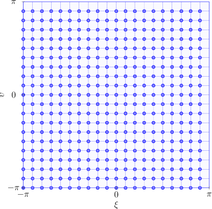
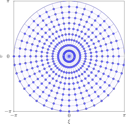
Figure 1: The above images depict all the points contained in two of the discrete domains described in the Introduction. Left: Cartesian Fourier Domain $\mathfrak{C}_{20,20}$. Right: Polar Fourier Domain $\mathfrak{P}_{20,20}$.

Note that, for $\mu$ and $\nu$ positive integers, $\mathfrak{C}_{M,N}\subset\mathfrak{C}_{\mu M,\nu N}$. Thus, it is possible to add new points to a CFD, but this demands at least doubling the DFT domain’s cardinality, for otherwise the samples of the DTFT computed at the points of $\mathfrak{C}_{M,N}$ will not be included in a new domain $\mathfrak{C}_{M^{\prime},N^{\prime}}$ unless both $\nicefrac{{M^{\prime}}}{{M}}$ and $\nicefrac{{N^{\prime}}}{{N}}$ are positive integers. This prevents incremental inclusion of a small amount of new sample points since, for using a CFD of slightly larger cardinality, the sample points of the smaller CFD will not be part of the larger domain.

Moreover, in some applications a radial sampling scheme of the Fourier space may be desirable, such as in MRI [11, 12], or unavoidable, such as in Computerized Tomography (CT) [13, 14], in which case the efficient computation of the DTFT for such a radial set of points is useful. Therefore, for these applications we may need to consider the evaluation of the DFT over a Polar Fourier Domain (PFD) $\mathfrak{P}_{M,N}$, defined by (see Figure 1, right)

$$\mathfrak{P}_{M,N}:=\Biggl{\{}\Biggl{(}\frac{2\pi I}{M}\cos\frac{\pi J}{N},\frac{2\pi I}{M}\sin\frac{\pi J}{N}\Biggr{)}:J {}\in\{0,1,\dots,N-1\}.$$

$$\text{and}\quad I\in\left\{-\nicefrac{{M}}{{2}},-\nicefrac{{M}}{{2}}+1,\dots,\nicefrac{{M}}{{2}}-1\right\}\Biggr{\}}.$$

Reasonably fast and accurate techniques are available that can evaluate $\mathcal{D}[\boldsymbol{x}]$ over a PFD [15, 16]. For a PFD, as was the case with the CFDs, no obvious way is available for including a small number of extra points in the domain. Instead, once more an inclusion of the form $\mathfrak{P}_{M,N}\subset\mathfrak{P}_{\mu M,\nu N}$ holds for positive integers $\mu$ and $\nu$, which is again of little practical value in many applications.

In the remainder of this introduction, we present the details of the newly proposed domains (the GALFDs), which have the flexibility of the Golden Angle Polar Fourier Domains (GAPFDs) and the benefit of the fast and accurate computation of the DFT over a Linogram Fourier Domain (LFD). Both the GAPFD and the LFD are presented below to motivate our choices, after which we introduce the new GALFD domains. Section 2 provides the mathematical theory required for the development of the technique, named GALE, that we propose for the approximate computation of the DFT over various domains, including the GALFD. Section 3 discusses the details of turning the theory into a computational methodology. Section 4 reports on our numerical experiments using both simulated data and actual MRI data. Section 5 gives our conclusions. The appendices provide (for the sake of completeness) some notations and algorithms that are either standard or well known and also a discussion of the relevance of our work to practical MRI in medicine.

1.2 The Linogram Fourier Domain

We define the subset $\mathfrak{L}_{M,N}$ of the real plane, called an LFD, by $\mathfrak{L}_{M,N}:=\mathfrak{H}_{M,N}\cup\mathfrak{V}_{M,N}$, where the sets $\mathfrak{H}_{M,N}$, and $\mathfrak{V}_{M,N}$ are given according to

$$\mathfrak{H}_{M,N}:=\Biggl{\{}\Biggl{(}\frac{2\pi I}{M},\frac{2\pi I}{M}\frac{4J}{N}\Biggr{)}:J\in\{-\nicefrac{{N}}{{4}} {}+1,-\nicefrac{{N}}{{4}}+2,\dots,\nicefrac{{N}}{{4}}\}$$

$$\text{and}\quad I\in\left\{-\nicefrac{{M}}{{2}},-\nicefrac{{M}}{{2}}+1,\dots,\nicefrac{{M}}{{2}}-1\right\}\Biggr{\}},$$

$$\mathfrak{V}_{M,N}:=\Biggl{\{}\Biggl{(}\frac{2\pi I}{M}\frac{4J}{N},\frac{2\pi I}{M}\Biggr{)}:J\in\{-\nicefrac{{N}}{{4}} ,-\nicefrac{{N}}{{4}}+1,\dots,\nicefrac{{N}}{{4}}-1\}$$

$$\text{and}\quad I\in\left\{-\nicefrac{{M}}{{2}}+1,-\nicefrac{{M}}{{2}}+2,\dots,\nicefrac{{M}}{{2}}\right\}\Biggr{\}}.$$

(See [13, (9.27), (9.28)]). An LFD is comprised of the intersections of $M$ equally spaced concentric squares and $N$ rays going through the origin, totaling $(M-1)N+1$ different points. Figure 2, left, shows an example of such a domain. As before, it is not possible to add just a small number of points to an LFD, even though for positive integers $\mu$ and $\nu$ we have $\mathfrak{L}_{M,N}\subset\mathfrak{L}_{\mu M,\nu N}$.

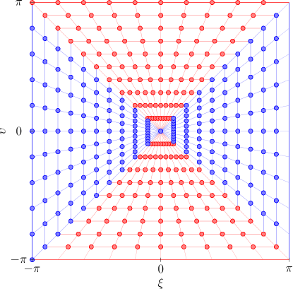
Figure 2: Left: The LFD $\mathfrak{L}_{20,20}$. The points of $\mathfrak{V}_{20,20}$ are displayed in red and the points of $\mathfrak{H}_{20,20}$ are displayed in blue. Right: Graphical representation of the GALFD $\mathfrak{N}_{20,20}$. The LRFSs with $\theta\in[\nicefrac{{\pi}}{{4}},\nicefrac{{3\pi}}{{4}})$ are shown in red and LRFSs with $\theta\in[\nicefrac{{3\pi}}{{4}},\nicefrac{{5\pi}}{{4}})$ are shown in blue.

Because of the Fourier Slice Theorem [13, (9.7)], the mathematics of CT allows us to think of the sampling obtained by a CT scanner as equivalent to a sampling of the Fourier space. Unlike in MRI, where direct acquisition of samples of the Fourier space is possible in arbitrary patterns, it is not possible to obtain directly the DFT over a CFD from CT data, due to the nature of the technique, but it is indeed possible to obtain Fourier samples over a PFD or over an LFD. Inversion of PFD data, however, requires certain approximations to be made or the use of computationally more expensive operations than just numerical Fourier transformations. On the other hand, inversion of LFD data is not only theoretically possible [5], but is also precise and computationally effective in practice [6]. In [7] LFDs appeared in the literature for the first time in connection with an MRI application. Efficient computation of the forward operator $\mathrm{D}_{\mathfrak{L}_{M,N}}\boldsymbol{x}$ is also discussed in [17], where the DFT over an LFD is named the Pseudo Polar Fourier Transform.

1.3 The Golden Angle Polar Fourier Domain

[width=0.5autoplay,loop]1gapfd_020

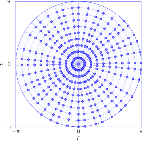
Figure 3: Left: Animation of the sequence of GAPFDs $\{\mathfrak{G}_{20,0},\mathfrak{G}_{20,1},\dots,\mathfrak{G}_{20,20}\}$, showing successive inclusion of the golden-angle spaced rays (JavaScript capable PDF viewer is required). Right: The GAPFD $\mathfrak{G}_{20,20}$.

The golden angle is $\Theta:=\nicefrac{{\pi}}{{\phi}}$, where $\phi:=\nicefrac{{\left(1+\sqrt{5}\right)}}{{2}}$ is the golden ratio. We then define the GAPFD $\mathfrak{G}_{M,N,\Theta_{0}}$ by

$$\mathfrak{G}_{M,N,\Theta_{0}}:=\Biggl{\{}\Biggl{(}\frac{2\pi I}{M}\cos\theta_{J},\frac{2\pi I}{M}\sin\theta_{J}\Biggr{)}:J {}\in\{0,1,\dots,N-1\}$$

$$\text{and}\quad I\in\left\{-\nicefrac{{M}}{{2}},-\nicefrac{{M}}{{2}}+1,\dots,\nicefrac{{M}}{{2}}-1\right\}\Biggr{\}},$$

where $\theta_{J}:=\left(\Theta_{0}+J\Theta\right)$, with $\Theta_{0}\in[0,2\pi]$. In principle, there is no reason to choose $\Theta$ to be $\nicefrac{{\pi}}{{\phi}}$. For example, the PFD $\mathfrak{P}_{M,N}$ would be equal to a rotation of the GAPFD $\mathfrak{G}_{M,N,\Theta_{0}}$ if $\Theta$ was replaced by $\nicefrac{{\pi}}{{N}}$. However, a GAPFD offers the advantages that the fine inclusion $\mathfrak{G}_{M,N,\Theta_{0}}\subset\mathfrak{G}_{M,N+1,\Theta_{0}}$ holds and that all of the GAPFDs present almost evenly distributed rays in the Fourier space [1].

These two properties together are of practical significance. They mean that new data can be incrementally added to an existing GAPFD sampling, as illustrated in Figure 3, in order to improve reconstruction while maintaining the overall structure of the dataset, a property that has been taken advantage of in several applications, see [2, 3, 4] and references therein for more on this subject.

1.4 The Golden Angle Linogram Fourier Domain

We now present our proposed family of domains, of which each member will be named a Golden Angle Linogram Fourier Domain (GALFD). A GALFD is an intermediate between an LFD and a GAPFD. It shares with an LFD the arrangement of the points of each of its rays into concentric squares, but unlike an LFD, the rays are distributed following the same golden angle spacing of a GAPFD. This way we retain the practical advantages of a GAPFD in comparison to a PFD in applications, while computation of the DFT over a GALFD can be performed more efficiently and accurately than computation of the DFT over a GAPFD or a PFD. How to perform the computation of the DFT over a GALFD is the subject of the next two sections.

We first define a Linogram Ray Fourier Subdomain (LRFS) $\mathfrak{R}_{M,\sigma}(\theta)$ for a positive even integer $M$, $\sigma\in\mathbb{R}$, and $\theta\in[\nicefrac{{\pi}}{{4}},\nicefrac{{5\pi}}{{4}})$. Then a GALFD is defined as a union of such subdomains. The definition of an LRFS is as follows:

$$\mathfrak{R}_{M,\sigma}(\theta)=\left\{\begin{array}[]{l}\biggl{\{}\biggl{(}\frac{2\pi I}{M}+\sigma,\left(\frac{2\pi I}{M}+\sigma\right)\tan\theta\biggr{)}:I\in\left\{-\nicefrac{{M}}{{2}},-\nicefrac{{M}}{{2}}+1,\dots,\nicefrac{{M}}{{2}}-1\right\}\biggr{\}}\\ \qquad\qquad\qquad\qquad\qquad\qquad\qquad\qquad\qquad\qquad\quad\text{if }\theta\in\left[\nicefrac{{3\pi}}{{4}},\nicefrac{{5\pi}}{{4}}\right),\\ \biggl{\{}\biggl{(}\left(\frac{2\pi I}{M}-\sigma\right)\cot\theta,\frac{2\pi I}{M}-\sigma\biggr{)}:I\in\left\{-\nicefrac{{M}}{{2}}+1,-\nicefrac{{M}}{{2}}+2,\dots,\nicefrac{{M}}{{2}}\right\}\biggr{\}}\\ \qquad\qquad\qquad\qquad\qquad\qquad\qquad\qquad\qquad\qquad\quad\ \text{if }\theta\in\left[\nicefrac{{\pi}}{{4}},\nicefrac{{3\pi}}{{4}}\right).\end{array}\right.$$ (2)

Let the angle constraining operator $\Lambda:\mathbb{R}\to\left[\nicefrac{{\pi}}{{4}},\nicefrac{{5\pi}}{{4}}\right)$ be given by

$$\Lambda(\theta):=\left(\theta-\nicefrac{{\pi}}{{4}}\right)\%\pi+\nicefrac{{\pi}}{{4}},$$

where $a\%b$ is, for real numbers $a$ and $b$, the remainder of the division of $a$ by $b$. The range $\left[\nicefrac{{\pi}}{{4}},\nicefrac{{5\pi}}{{4}}\right)$ is conventional; we could have chosen any half-open interval of length $\pi$. We define the GALFD $\mathfrak{N}_{M,N,\Theta_{0},\sigma}$ by (see Figure 2, right, for an example)

$$\mathfrak{N}_{M,N,\Theta_{0},\sigma}:=\bigcup_{J=0}^{N}\mathfrak{R}_{M,\sigma}\left(\Lambda\left(\Theta_{0}+J\Theta\right)\right).$$

Whenever possible, we simplify the notation by using $\mathfrak{N}_{M,N}:=\mathfrak{N}_{M,N,\nicefrac{{\pi}}{{2}},\nicefrac{{\pi}}{{M}}}$.

In the next sections we describe our method for efficiently computing the DFT over a GALFD. Section 2 presents the required mathematical development, including an upper bound on the incurred approximation error. Section 3 provides a precise algorithmic formulation for the whole procedure and discusses floating point operations count and memory-related issues.

2 Mathematical Foundations

In the present section we discuss the mathematical foundations of the method we propose for the computation of the DFT over an LRFS. We give an approximation of $\mathrm{D_{\mathfrak{R}_{M,\sigma}(\theta)}}\left[\boldsymbol{x}\right]$ for any fixed $\theta\in\left[\nicefrac{{\pi}}{{4}},\nicefrac{{3\pi}}{{4}}\right)$ and $\boldsymbol{x}\in\mathbb{C}^{mn}$. We assume that $M\geq m$, and that $M$ is even. The evenness assumption is used only for simplicity of exposition, but $M\geq m$ is useful for computational efficiency. The reasoning for $\theta\in\left[\nicefrac{{3\pi}}{{4}},\nicefrac{{5\pi}}{{4}}\right)$ is analogous and consequently we do not present its repetitive details. In the algorithmic description of the next section, however, the computational details are given in a concise but complete way.

Consider an arbitrary $\theta\in\left[\nicefrac{{\pi}}{{4}},\nicefrac{{3\pi}}{{4}}\right)$ and write $c=\cot\theta$. We proceed from the definition

$$\mathcal{D}[\boldsymbol{x}]\left(\left(\frac{2\pi I}{M}-\sigma\right)c,\frac{2\pi I}{M}-\sigma\right) {}=\sum_{i=0}^{m-1}\sum_{j=0}^{n-1}x_{i,j}e^{-\imath\left(j\left(\frac{2\pi I}{M}-\sigma\right)c+i\left(\frac{2\pi I}{M}-\sigma\right)\right)}$$

$${}=\sum_{j=0}^{n-1}\sum_{i=0}^{m-1}x_{i,j}e^{-\imath\left(j\left(\frac{2\pi I}{M}-\sigma\right)c+i\left(\frac{2\pi I}{M}-\sigma\right)\right)}$$

$${}=\sum_{j=0}^{n-1}e^{-\imath j\left(\frac{2\pi I}{M}-\sigma\right)c}\sum_{i=0}^{m-1}x_{i,j}e^{-\imath i\left(\frac{2\pi I}{M}-\sigma\right)}$$

$${}=\sum_{j=0}^{n-1}X_{I,j}e^{-\imath j\left(\frac{2\pi I}{M}-\sigma\right)c},$$

where (note that this is a one-dimensional discrete Fourier transform of $x_{i,j}$ with respect to $i$, refer to A for details)

$$X_{I,j}:=\sum_{i=0}^{m-1}x_{i,j}e^{\imath i\sigma}e^{-\imath i\frac{2\pi I}{M}}.$$ (3)

Now we rewrite these computations as

$$\mathcal{D}[\boldsymbol{x}]\left(\left(\frac{2\pi I}{M}-\sigma\right)c,\frac{2\pi I}{M}-\sigma\right)=\sum_{j=0}^{n-1}X_{I,j}e^{-\imath j\frac{2\pi\eta}{N_{L}}\alpha_{I}},$$ (4)

where $N_{L}\geq 2n$ is an integer divisible by $4$, $\eta=\nicefrac{{cN_{L}}}{{4}}$ and $\alpha_{I}=\nicefrac{{4I}}{{M}}-\nicefrac{{2\sigma}}{{\pi}}$. If $\eta$ were an integer with $\eta\in\left\{-\nicefrac{{N_{L}}}{{4}},-\nicefrac{{N_{L}}}{{4}}+1,\dots,\nicefrac{{N_{L}}}{{4}}-1\right\}$, then the right hand side of (4) would be a part of the output of a Chirp-Z Transform (CZT) [18] of length $\nicefrac{{N_{L}}}{{2}}$, which can be efficiently computed with the use of one FFT and one Inverse FFT (IFFT). This is what makes the computation of the DFT over an LFD efficient. However, in the LRFS case that we are considering, where $c=\cot\theta$ is not constrained to specific values in the interval [-1,1], $\eta$ is not necessarily an integer, and we need an appropriate theoretical tool to help us to deal with this situation.

As a preliminary step, we provide the definition of the Continuous Fourier Transform (CFT). Let $f:\mathbb{R}^{n}\to\mathbb{C}$ be an absolutely integrable function, its CFT $\hat{f}:\mathbb{R}^{n}\to\mathbb{C}$ is

$$\hat{f}(\boldsymbol{\omega}):=\mathcal{F}[f](\boldsymbol{\omega}):=\int_{\mathbb{R}^{n}}f(\boldsymbol{x})e^{-\imath\langle\boldsymbol{x},\boldsymbol{\omega}\rangle}\mathrm{d}\boldsymbol{x},$$

where $\langle\boldsymbol{x},\boldsymbol{\omega}\rangle$ is the inner product between $\boldsymbol{x}\in\mathbb{R}^{n}$ and $\boldsymbol{\omega}\in\mathbb{R}^{n}$. The following is a very useful result due to Fourmont [19]. Since the differences in our statement are due only to the notation and to the normalization of the CFT, we refer the reader to [19, Proposition 1] for a proof.

Theorem 1.

Let $\tau\in\mathbb{R}$ and $\delta\in\mathbb{R}$ be such that $0<\nicefrac{{\pi}}{{\delta}}<\tau<2\pi-\nicefrac{{\pi}}{{\delta}}$. Let also $W:\mathbb{R}\to\mathbb{R}$ be continuous and piecewise continuously differentiable in $[-\tau,\tau]$, vanishing outside $[-\tau,\tau]$ and nonzero in $\left[-\nicefrac{{\pi}}{{\delta}},\nicefrac{{\pi}}{{\delta}}\right]$, and let $\hat{W}:\mathbb{R}\to\mathbb{R}$ be its Fourier transform. Then, for $\zeta\in\mathbb{R}$ and $|t|\leq\nicefrac{{\pi}}{{\delta}}$, we have

$$e^{-\imath\zeta t}=\frac{1}{2\pi W(t)}\sum_{J\in\mathbb{Z}}\hat{W}(\zeta-J)e^{-\imath Jt}.$$

As an immediate consequence of the above equality, we have, for $|t-\varpi|\leq\pi/\delta$,

$$e^{-\imath\zeta t} {}=e^{-\imath\zeta\varpi}e^{-\imath\zeta(t-\varpi)}$$ (5)

$${}=\frac{e^{-\imath\zeta\varpi}}{2\pi W(t-\varpi)}\sum_{J\in\mathbb{Z}}\hat{W}(\zeta-J)e^{-\imath J(t-\varpi)}$$

$${}=\frac{1}{2\pi W(t-\varpi)}\sum_{J\in\mathbb{Z}}\hat{W}(\zeta-J)e^{-\imath(\zeta-J)\varpi}e^{-\imath Jt}.$$

Now, let $t_{j}^{I}:=\left(\nicefrac{{(2\pi j)}}{{N_{L}}}\right)\alpha_{I}$ (where $\alpha_{I}$ is as in (4)) and

$$\varpi_{I}:=\frac{\pi(n-1)}{N_{L}}\alpha_{I}.$$ (6)

At this point, we must introduce the constraint $|\sigma|<\nicefrac{{\pi}}{{(n-1)}}$. If this condition is true, taking into consideration that $N_{L}\geq 2n,$ that $j\in\{0,1,\dots,n-1\}$, and that $|I|\leq\nicefrac{{M}}{{2}}$, we have

$$|t_{j}^{I}-\varpi_{I}| {}=\left|\frac{\pi\alpha_{I}}{N_{L}}\left(2j-(n-1)\right)\right|=\frac{\pi}{N_{L}}\left|\frac{4I}{M}-\frac{2\sigma}{\pi}\right|\left|2j-(n-1)\right|$$ (7)

$${}\leq\frac{\pi}{N_{L}}\left|\frac{4I}{M}-\frac{2\sigma}{\pi}\right|(n-1)\leq\frac{\pi}{2}\left|\frac{4I}{M}-\frac{2\sigma}{\pi}\right|\frac{n-1}{n}$$

$${}\leq\frac{\pi}{2}\left(\left|\frac{4I}{M}\right|+\frac{2|\sigma|}{\pi}\right)\frac{n-1}{n}\leq\frac{\pi}{2}\left(2+\frac{2|\sigma|}{\pi}\right)\frac{n-1}{n}$$

$${}=\pi\left(1+\frac{|\sigma|}{\pi}\right)\frac{n-1}{n}<\pi\left(1+\frac{1}{n-1}\right)\frac{n-1}{n}=\pi.$$

Now, define, for an $\varepsilon\in(0,1)$ such that $\varepsilon\approx 1$ (we use the specific value $\varepsilon=1-10^{-4}$),

$$\tau_{I}:=\pi+\varepsilon\left(\pi-|\varpi_{I}|\right).$$ (8)

Note that a computation similar to (7) gives $|\varpi_{I}|<\pi$; therefore, because of the definition of $\tau_{I}$, we have $\pi<\tau_{I}<2\pi$. Thus, if some $W_{I}:\mathbb{R}\to\mathbb{R}$ is smooth for $t\in\left[-\tau_{I},\tau_{I}\right]$, $W_{I}(t)\neq 0$ for $t\in\left(-\tau_{I},\tau_{I}\right)$, and $W_{I}(t)=0$ for $t\notin\left(-\tau_{I},\tau_{I}\right)$, then $W_{I}$ satisfies all conditions for $W$ in the statement of Theorem 1 with any $\delta>\max\left\{\nicefrac{{\pi}}{{\tau_{I}}},\nicefrac{{\pi}}{{\left(2\pi-\tau_{I}\right)}}\right\}$. Hence, in view of (7), (5) can be used with $W=W_{I}$, $t=t_{j}^{I}$, $\zeta=\eta$, and $\varpi=\varpi_{I}$ inside of (4) in order to yield

$$\mathcal{D}[\boldsymbol{x}]\Biggl{(}\left(\frac{2\pi I}{M}-\sigma\right)c,\frac{2\pi I}{M} {}-\sigma\Biggr{)}$$ (9)

$${}=\sum_{j=0}^{n-1}X_{I,j}e^{-\imath\eta t_{j}^{I}}$$

$${}=\sum_{j=0}^{n-1}X_{I,j}\frac{1}{2\pi W_{I}\left(t_{j}^{I}-\varpi_{I}\right)}\sum_{J\in\mathbb{Z}}\hat{W}_{I}(\eta-J)e^{-\imath(\eta-J)\varpi_{I}}e^{-\imath Jt_{j}^{I}}$$

$${}=\frac{1}{2\pi}\sum_{J\in\mathbb{Z}}\hat{W}_{I}(\eta-J)e^{-\imath(\eta-J)\varpi_{I}}\sum_{j=0}^{n-1}X_{I,j}\frac{1}{W_{I}\left(t_{j}^{I}-\varpi_{I}\right)}e^{-\imath Jt_{j}^{I}}$$

$${}=\frac{1}{2\pi}\sum_{J\in\mathbb{Z}}\frac{\hat{W}_{I}(\eta-J)}{e^{\imath(\eta-J)\varpi_{I}}}\sum_{j=0}^{n-1}X_{I,j}\frac{1}{W_{I}\left(t_{j}^{I}-\varpi_{I}\right)}e^{-\imath j\frac{2\pi J}{N_{L}}\alpha_{I}}.$$

This means that the values of the DTFT at the desired points can be approximated by a sum

$$\mathcal{D}[\boldsymbol{x}]\Biggl{(}\left(\frac{2\pi I}{M}-\sigma\right)c,\frac{2\pi I}{M} {}-\sigma\Biggr{)}$$ (10)

$${}\approx\frac{1}{2\pi}\sum_{|J-\eta|\leq S}\frac{\hat{W}_{I}(\eta-J)}{e^{\imath(\eta-J)\varpi_{I}}}\sum_{j=0}^{n-1}X_{I,j} \frac{1}{W_{I}\left(t_{j}^{I}-\varpi_{I}\right)}e^{-\imath j\frac{2\pi J}{N_{L}}\alpha_{I}}$$

$$\qquad\qquad\ {}=:D_{I,N_{L},S}(\theta),$$

where the positive integer $S$, which dictates the number of terms in the truncated sum, is a parameter determining the accuracy of the approximation. Another such parameter is the length of the support of $W_{I}$. We return to this topic when we derive an upper bound for the approximation error.

Now we tackle the issue of determining the “window functions” $W_{I}:\mathbb{R}\to\mathbb{R}$ that satisfy the conditions of Theorem 1. Of course, there is some freedom in the selection of these window functions and many have been proposed and used in the literature. Among the most successful and popular is the family of Kaiser-Bessel [20] Window Functions (KBWFs). Members of this family of functions have finite support as required for the theorem to hold, and they also have the desirable property that the infinite series on the right-hand side of (5) converges very quickly, thus making the approximation by a finite summation precise even when only a few terms are used. The definition of a KBWF is as follows. For parameters $\beta\in\mathbb{R}$ and $\tau\in\mathbb{R}$,

$$K_{\beta,\tau}(t):=\left\{\begin{array}[]{ll}{\displaystyle\frac{\mathcal{I}_{0}\left(\beta\sqrt{1-(t/\tau)^{2}}\right)}{\mathcal{I}_{0}(\beta)},}&\quad\text{if}\quad|t|\leq\tau,\\ 0,&\quad\text{otherwise,}\end{array}\right.$$

where $\mathcal{I}_{0}:\mathbb{R}\to\mathbb{R}$ is the (real) modified zero-order cylindrical Bessel function. Note that

$$\hat{K}_{\beta,\tau}(\omega)=\frac{2\tau}{\mathcal{I}_{0}(\beta)}\frac{\sinh\left(\beta\sqrt{1-(\omega\tau/\beta)^{2}}\right)}{\beta\sqrt{1-(\omega\tau/\beta)^{2}}}.$$

In our methods we use specifically the following window functions: For $\beta_{I}:=S\tau_{I}$,

$$W_{I}:=K_{\beta_{I},\tau_{I}}.$$ (11)

Figure 4 shows examples of the Kaiser-Bessel window functions described above for some combination of parameters.

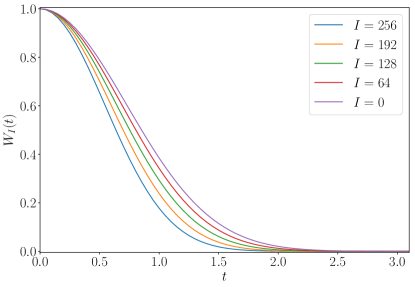
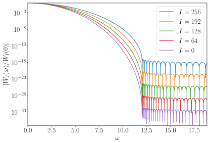
Figure 4: Plots of Kaiser-Bessel window functions (left) and respective Fourier transforms (right) for several values of $I$ with parameters $m=n=M=512$, $N_{L}=2.25m$, $\sigma=\nicefrac{{\pi}}{{M}}$, and $\epsilon=1-10^{-4}$.

We now present our upper bound for the approximation error due to the truncation (10).

Theorem 2.

Let $\theta\in\left[\nicefrac{{\pi}}{{4}},\nicefrac{{3\pi}}{{4}}\right),$ $|\sigma|<\nicefrac{{\pi}}{{(n-1)}}$, $\boldsymbol{x}\in\mathbb{C}^{mn}$, $M\geq m$, $N_{L}\geq 2n$, $1<S\leq 15$, $|I|\leq\nicefrac{{M}}{{2}}$, $\varpi_{I}$ as in (6), $\tau_{I}$ as in (8), and $D_{I,N_{L},S}(\theta)$ as in (10) with (11), then

$$\left|\mathcal{D}[\boldsymbol{x}]\left(\left(\frac{2\pi I}{M}-\sigma\right)\cot\theta,\frac{2\pi I}{M}-\sigma\right)-D_{I,N_{L},S}(\theta)\right|\leq\frac{29.5\|\boldsymbol{x}\|_{1}}{\pi\mathcal{I}_{0}\left(S\sqrt{\tau_{I}^{2}-\varpi_{I}^{2}}\right)},$$ (12)

where $\|\boldsymbol{x}\|_{1}:=\sum_{i=0}^{m-1}\sum_{j=0}^{n-1}\left|x_{i,j}\right|$.

Proof.

Let us first consider the difference below (notice that, although omitted from the notation, $\eta$ is a function of $N_{L}$ and $\theta$, and $W_{I}$ depends on $N_{L}$ through the parameter $\tau_{I}$):

$$\varepsilon_{j}^{I,N_{L},S}(\theta):=e^{-\imath\eta t_{j}^{I}}-\frac{1}{2\pi W_{I}\left(t_{j}^{I}-\varpi_{I}\right)}\sum_{|J-\eta|\leq S}\hat{W}_{I}(\eta-J)e^{-\imath(\eta-J)\varpi_{I}}e^{-\imath Jt_{j}^{I}}.$$ (13)

Notice that $\varepsilon_{j}^{I,N_{L},S}(\theta)$ is well defined since (7) and (8) imply that $\left|t_{j}^{I}-\varpi_{I}\right|<\tau_{I}$, which in turn, following definition (11), implies that $W_{I}\left(t_{j}^{I}-\varpi_{I}\right)>0$. Because of (5) we have

$$\left|\varepsilon_{j}^{I,N_{L},S}(\theta)\right| {}=\left|\frac{1}{2\pi W_{I}\left(t_{j}^{I}-\varpi_{I}\right)}\sum_{|J-\eta|>S}\hat{W}_{I}(\eta-J)e^{-\imath(\eta-J)\varpi_{I}}e^{-\imath Jt_{j}^{I}}\right|$$

$${}=\frac{1}{2\pi W_{I}\left(t_{j}^{I}-\varpi_{I}\right)}\left|\sum_{|J-\eta|>S}\hat{W}_{I}(\eta-J)e^{\imath(\eta-J)(t_{j}^{I}-\varpi_{I})}\right|,$$

since $\left|e^{-\imath\eta t_{j}^{I}}\right|=1$. By denoting $\ell=\eta-J$ and $t=t_{j}^{I}-\varpi_{I}$ we get

$$\left|\varepsilon_{j}^{I,N_{L},S}(\theta)\right|=\frac{1}{2\pi W_{I}(t)}\left|\sum_{|\ell|>S}\hat{W}_{I}(\ell)e^{\imath\ell t}\right|.$$ (14)

Now consider the specific window functions we use. Because $W_{I}=K_{\beta_{I},\tau_{I}}$ where $\beta_{I}=S\tau_{I}$,

$$\hat{W}_{I}(\omega)=\frac{2}{\mathcal{I}_{0}(\beta_{I})}\frac{\sinh\left(\tau_{I}\sqrt{S^{2}-\omega^{2}}\right)}{\sqrt{S^{2}-\omega^{2}}}.$$

For the specific case where $\ell>S$, the square roots are imaginary and we can write this as

$$\hat{W}_{I}(\ell)=\frac{2}{\mathcal{I}_{0}(\beta_{I})}\frac{\sin\left(\tau_{I}\sqrt{\ell^{2}-S^{2}}\right)}{\sqrt{\ell^{2}-S^{2}}}.$$

Thus, using this equality in (14) and considering that $W_{I}=K_{\beta_{I},\tau_{I}}$ we get, because $|t|<\tau_{I}$,

$$\left|\varepsilon_{j}^{I,N_{L},S}(\theta)\right|=\frac{1}{\pi\mathcal{I}_{0}\left(S\sqrt{\tau_{I}^{2}-t^{2}}\right)}\left|\sum_{|\ell|>S}\frac{\sin\left(\tau_{I}\sqrt{\ell^{2}-S^{2}}\right)}{\sqrt{\ell^{2}-S^{2}}}\right|.$$

Now we can apply [21, Corollar 2.5.12], which holds for $1<S\leq 15$, in order to obtain

$$\left|\varepsilon_{j}^{I,N_{L},S}(\theta)\right|\leq\frac{29.5}{\pi\mathcal{I}_{0}\left(S\sqrt{\tau_{I}^{2}-t^{2}}\right)}.$$

Now, notice that because the Bessel function $\mathcal{I}_{0}$ is monotonically increasing, the denominator is minimized when $t^{2}=\left(t_{j}^{I}-\varpi_{I}\right)^{2}$ is as close as possible to $\tau_{I}^{2}$. Equivalently, because $\left(t_{j}^{I}-\varpi_{I}\right)^{2}<\pi^{2}<\tau_{I}^{2}$ (see (7) and the definition of $\tau_{I}$ in (8)), this occurs when $\left(t_{j}^{I}-\varpi_{I}\right)^{2}$ is maximized over $j\in\{0,1,\dots,n-1\}$, which occurs when $j=0$ or when $j=(n-1)$ because

$$t_{j}^{I}-\varpi_{I}=\frac{\pi\alpha_{I}}{N_{L}}\left(2j-(n-1)\right).$$

From the definition of $\varpi_{I}$ in (6) it follows that

$$\left(t_{0}^{I}-\varpi_{I}\right)^{2}=\left(t_{(n-1)}^{I}-\varpi_{I}\right)^{2}=\varpi_{I}^{2}.$$

Therefore we obtain the following upper bound for $\varepsilon_{j}^{I,N_{L},S}(\theta)$ that is uniform in $\theta$ and $j$:

$$\left|\varepsilon_{j}^{I,N_{L},S}(\theta)\right|\leq\frac{29.5}{\pi\mathcal{I}_{0}\left(S\sqrt{\tau_{I}^{2}-\varpi_{I}^{2}}\right)}=:\varepsilon_{I,N_{L},S}.$$

Defining $\delta_{j}^{I,N_{L},S}(\theta)$ as below and using (9), (10), and (13) we complete the proof:

$$\delta_{j}^{I,N_{L},S}(\theta):=\left|\mathcal{D}[\boldsymbol{x}]\biggl{(}\biggl{(}\frac{2\pi I}{M}-\sigma\biggr{)}\cot\theta,\frac{2\pi I}{M}-\sigma\biggr{)}-D_{I,N_{L},S}(\theta)\right|.$$

$$\delta_{j}^{I,N_{L},S}(\theta) {}=\left|\sum_{j=0}^{n-1}X_{I,j}\varepsilon_{j}^{I,N_{L},S}(\theta)\right|$$

$${}\leq\left|\sum_{j=0}^{n-1}X_{I,j}\right|\varepsilon_{I,N_{L},S}\leq\sum_{j=0}^{n-1}\left|X_{I,j}\right|\varepsilon_{I,N_{L},S}$$

$${}=\sum_{j=0}^{n-1}\left|\sum_{i=0}^{m-1}x_{i,j}e^{\imath i\sigma}e^{-\imath i\frac{2\pi I}{M}}\right|\varepsilon_{I,N_{L},S}$$

$${}\leq\varepsilon_{I,N_{L},S}\sum_{j=0}^{n-1}\sum_{i=0}^{m-1}\left|x_{i,j}\right|.$$

∎

In the next section we give details of how to turn the above development into practical algorithms. Here we discuss some aspects of the error bound that we have just obtained. Consider fixed $N_{L}$ and $S$. We notice that $\tau_{I}^{2}-\varpi_{I}^{2}$ is larger for the lower frequency elements of the GALFD (i.e., $I$ close to $0$). This observation is important because the error bound in (12) is smaller when $\tau_{I}^{2}-\varpi_{I}^{2}$ is larger. This means that, for a given computational effort (which, for fixed $m$, $n$, and $M$, depends only on $N_{L}$ and $S$), we get better accuracy in the region of the spectrum where data are usually more reliable in practical applications. This is also interesting in the scenario where one wishes to vary $N_{L}$ and $S$ for each $I$, which could be easily considered in our theoretical framework, in order to obtain an overall desired accuracy with the smallest possible computational cost. For example, Figure 5 shows that the Fourier sample length $N_{L}$ becomes less important as $I$ gets close to zero, and could therefore be reduced in these regions, because there is a “natural oversampling” due to the fact that the samples used in the truncated sum get very close to each other in that region. Our approximation makes use of this fact by lengthening the size of the $W_{I}$ window support, thereby improving its decay in the Fourier domain and consequently reducing the precision loss caused by truncation of the infinite summation.

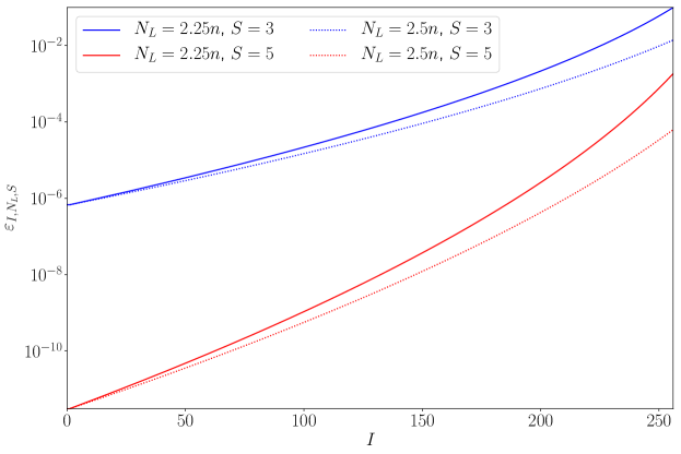
Figure 5: The error bound $\varepsilon_{I,N_{L},S}$ as a function of $I$ for indicated $N_{L}$ and $S$ ($M=m=n=512$, $\sigma=\pi/M$).

3 Computational Algorithm Formulation

At this point, the core of our strategy has been outlined. The first step consists of the computation of the $X_{I,j}$ for $I\in\{-\nicefrac{{M}}{{2}}+1,-\nicefrac{{M}}{{2}}+2,\dots,\nicefrac{{M}}{{2}}\}$ and $j\in\{0,1,\dots,n-1\}$ using $n$ FFTs of length $M$, see (3), and then multiplying the results by the weights $\nicefrac{{1}}{{W_{I}\left(t_{j}^{I}-\varpi_{I}\right)}}$, see (9). After this multiplication, the values

$$Z_{I,J}:=\sum_{j=0}^{n-1}X_{I,j}\frac{1}{W_{I}\left(t_{j}^{I}-\varpi_{I}\right)}e^{-\imath j\frac{2\pi J}{N_{L}}\alpha_{I}}$$ (15)

can be computed efficiently using $M$ CZTs, as we discuss below in B. An important detail that should not be overlooked is that, because $\eta$ can be very close to $\pm\nicefrac{{N_{L}}}{{4}}$, we may need $S+1$ extra points at each end of the output of the CZT for the right-hand side of (10) to be computable, and, thus, each CZT will have length $\nicefrac{{N_{L}}}{{2}}+2(S+1)$. Finally, the values of the estimates of the DFT at the desired points are computed by a linear combination of the previously-obtained values of $Z_{I,J}$, as in (10). In the appendices we describe for completeness two well known key computational elements that are used in our method. We leave the full description of our algorithm to Subsection 3.1 and we discuss its computational complexity in Subsection 3.2.

3.1 GALE: Approximating the DFT over a GALFD

Now we present GALE, the method that we propose for the computation of the DFT over a GALFD (an open source reference implementation can be downloaded from https://bitbucket.org/eshneto/gale/downloads/). We give an algorithm for the region $\theta\in\left[\nicefrac{{\pi}}{{4}},\nicefrac{{3\pi}}{{4}}\right)$ and explain later how to make use of the same computations in order to obtain the case $\theta\in\left[\nicefrac{{3\pi}}{{4}},\nicefrac{{5\pi}}{{4}}\right)$. Note that GALE is adaptable to other domains as well.

Before starting the presentation, we discuss some typographical conventions that are used in the description of the method. We denote non-scalar entities such as vectors, two-dimensional, or three-dimensional arrays of numbers by boldface letters, possibly with a subscript or with a superscript. If $\boldsymbol{x}\in\mathbb{C}^{mn}$ is a two-dimensional array with $m$ lines and $n$ columns, then $\boldsymbol{x}^{j}\in\mathbb{C}^{m}$ with $j\in\{0,1,\dots,n-1\}$ is the $j$-th column of $\boldsymbol{x}$, that is, $\boldsymbol{x}^{j}=\left(x_{0,j},x_{1,j},\dots,x_{m-1,j}\right)^{T}$. Likewise, $\boldsymbol{x}_{i}\in\mathbb{C}^{n}$ with $i\in\{0,1,\dots,m-1\}$ is the $i$-th row of $\boldsymbol{x}$ expressed as a column vector, that is, $\boldsymbol{x}_{i}=\left(x_{i,0},x_{i,1},\dots,x_{i,n-1}\right)^{T}$. Whenever there is a set of scalars indexed with subscripts and/or superscripts, a corresponding boldface letter represents the collection of those scalars. For example, $\boldsymbol{x}\in\mathbb{C}^{mn}$ is an entity that collects all scalars $x_{i,j}$. In another example, the algorithm may set values of $v_{i}^{I,K}$ for certain ranges of $I$, $K$, and $i$. In this case, $\boldsymbol{v}$ represents the set of all $v_{i}^{I,K}$ that were defined during the algorithm’s execution.

Algorithm 1 $\text{GALE-I}\left(\boldsymbol{\theta},m,n,M,N,N_{L},S,R_{1},R_{2},\sigma,\varepsilon\right)$

1:  for $i\in\{0,1,\dots,m-1\}$ do

2:        $p_{i}\leftarrow e^{\imath i\left(\frac{2\pi R_{1}}{M}+\sigma\right)}$

3:  for $I\in\{0,1,\dots,M-1\}$ do

4:        $\alpha_{I}\leftarrow\frac{4\left(I-R_{1}\right)}{M}-\frac{2\sigma}{\pi}$

5:        $(\hat{\boldsymbol{q}}^{I},\boldsymbol{r}^{I},\boldsymbol{s}^{I})\leftarrow\text{CZT-I}\left(n,\alpha_{I},N_{L},\nicefrac{{N_{L}}}{{2}}+2(S+1),R_{2}\right)$

6:        $\varpi_{I}\leftarrow\frac{\pi(n-1)}{N_{L}}\alpha_{I}$

7:        $\tau_{I}\leftarrow\pi+\varepsilon\left(\pi-|\varpi_{I}|\right)$

8:        for $j\in\{0,1,\dots,n-1\}$ do

9:              $t_{j}^{I}\leftarrow\frac{2\pi j}{N_{L}}\alpha_{I}$

10:              $r_{j}^{I}\leftarrow\frac{r_{j}^{I}}{K_{S\tau_{I},\tau_{I}}\left(t_{j}^{I}-\varpi_{I}\right)}$

11:        for $K\in\{0,1,\dots,N-1\}$ do

12:              $\eta_{K}\leftarrow\frac{N_{L}\cot\theta_{K}}{4}$

13:              $i\leftarrow 0$

14:              for $J\in\left\{\ell:\left|\ell-\eta_{K}\right|\leq S\right\}$ do

15:                    $v_{i}^{I,K}\leftarrow J+R_{2}$

16:                    $w_{i}^{I,K}\leftarrow\frac{\hat{K}_{S\tau_{I},\tau_{I}}\left(\eta_{K}-J\right)}{2\pi e^{\imath\left(\eta_{K}-J\right)\varpi_{I}}}$

17:                    $i\leftarrow i+1$

18:              $u_{I,K}\leftarrow i$

19:  return $(\boldsymbol{p},\hat{\boldsymbol{q}},\boldsymbol{r},\boldsymbol{s},\boldsymbol{u},\boldsymbol{v},\boldsymbol{w})$

Algorithm 2 $\text{GALE}\left(\boldsymbol{x},m,n,M,N,N_{L},S,\boldsymbol{p},\hat{\boldsymbol{q}},\boldsymbol{r},\boldsymbol{s},\boldsymbol{u},\boldsymbol{v},\boldsymbol{w}\right)$

1:  for $j\in\{0,1,\dots,n-1\}$ do

2:        for $i\in\{0,1,\dots,m-1\}$ do

3:              $x_{i,j}\leftarrow x_{i,j}p_{i}$

4:        $\boldsymbol{U}^{j}\leftarrow\text{FFT}\left(\boldsymbol{x}^{j},m,M\right)$

5:  for $I\in\{0,1,\dots,M-1\}$ do

6:        $\boldsymbol{V}_{I}\leftarrow\text{CZT}\left(\boldsymbol{U}_{I},n,\nicefrac{{N_{L}}}{{2}}+2(S+1),\hat{\boldsymbol{q}}^{I},\boldsymbol{r}^{I},\boldsymbol{s}^{I}\right)$

7:        for $K\in\{0,1,\dots,N-1\}$ do

8:              $Y_{I,K}\leftarrow 0$

9:              for $i\in\left\{0,1,\dots,u_{I,K}-1\right\}$ do

10:                    $J\leftarrow v_{i}^{I,K}$

11:                    $Y_{I,K}\leftarrow Y_{I,K}+w_{i}^{I,K}V_{I,J}$

12:  return $(\boldsymbol{Y})$

Now we discuss the specific algorithm GALE that we are introducing in the present paper. Algorithm 1 is the initialization phase, which is run only once for a combination of parameters $\boldsymbol{\theta}\in[\nicefrac{{\pi}}{{4}},\nicefrac{{3\pi}}{{4}})^{N}$, $m$, $n$, $M$, $N$, $N_{L}$, $S$, $R_{1}$, $R_{2}$, $\sigma$, and $\varepsilon$. Algorithm 2 uses the output of Algorithm 1 in order to compute an approximation to the DFT over the $\mathfrak{R}_{M,\sigma}(\theta_{K})$ of (2) for $K\in\{0,1,\dots,N-1\}$. Parameters $N_{L}$, $S$, and $\varepsilon$ influence the quality of the approximation. Parameters $m$, $n$, $M$, and $N$ are related to the dimensions of the image and the domain. Parameter $R_{1}$ determines the range $I\in\left\{-R_{1},-R_{1}+1,\dots,M-R_{1}-1\right\}$ of the domain in order to match the definition (2), and parameter $R_{2}$ determines the range $J\in\left\{-R_{2},-R_{2}+1,\dots,\nicefrac{{N_{L}}}{{2}}+2(S+1)-R_{2}-1\right\}$ of elements $Z_{I,J}$ from (15) that are going to be computed to be used in the truncated sum (10).

Assuming that we have run the initialization as

$$(\boldsymbol{p},\hat{\boldsymbol{q}},\boldsymbol{r},\boldsymbol{s},\boldsymbol{u},\boldsymbol{v},\boldsymbol{w})\leftarrow\text{GALE-I}\left(\boldsymbol{\theta},m,n,M,N,N_{L},S,R_{1},R_{2},\sigma,\varepsilon\right)$$

with $R_{1}=\nicefrac{{M}}{{2}}-1$ and $R_{2}=\nicefrac{{N_{L}}}{{4}}+S+1$, we analyze the output of

$$(\boldsymbol{Y})\leftarrow\text{GALE}\left(\boldsymbol{x},m,n,M,N,N_{L},S,\boldsymbol{p},\hat{\boldsymbol{q}},\boldsymbol{r},\boldsymbol{s},\boldsymbol{u},\boldsymbol{v},\boldsymbol{w}\right).$$

First notice that, because of the way $\boldsymbol{p}$ is initialized in Steps 1-2 of Algorithm 1, Steps 1-4 of Algorithm 2 store in the array $\boldsymbol{U}\in\mathbb{C}^{Mn}$ the elements $U_{I,J}=X_{I-R_{1},j}$, with $X_{I-R_{1},j}$ as defined in (3), for $I\in\{0,1,\dots,M-1\}$ and $j\in\{0,1,\dots,n-1\}$. Fix an $I\in\{0,1,\dots,M-1\}$ and notice that Step 10 of Algorithm 1 modifies the $\boldsymbol{r}^{I}$ that was previously obtained at Step 5 of Algorithm 1 in a way such that Step 6 of Algorithm 2 computes $V_{I,J}=Z_{I-R_{1},J-R_{2}}$, with $Z_{I-R_{1},J-R_{2}}$ as defined in (15), for $J\in\left\{0,1,\dots,\nicefrac{{N_{L}}}{{2}}+2(S+1)\right\}$. Fix a $K\in\{0,1,\dots,N-1\}$ and notice that the $u_{I,K}$ recorded in Step 18 of Algorithm 1 stores the number of terms in

$$\sum_{\left|J-\eta_{K}\right|\leq S}\frac{\hat{W}_{I}\left(\eta_{K}-J\right)}{2\pi e^{\imath\left(\eta_{K}-J\right)\varpi_{I}}}Z_{I,J}$$

of the approximation (10). Furthermore, according to Step 15 of Algorithm 1, the set $\left\{v_{0}^{I,K},\dots,v_{u_{I,K}-1}^{I,K}\right\}$ equals the set $\left\{J+R_{2}:\left|J-\eta_{K}\right|\leq S\right\}$ of the indices that go into the above summation, while Step 16 of Algorithm 1 ensures that $w_{i}^{I,K}=\frac{\hat{W}_{I}\left(\eta_{K}-J_{i}\right)}{2\pi e^{\imath\left(\eta_{K}-J_{i}\right)\varpi_{I}}}$, where $J_{i}:=v_{i}^{I,K}-R_{2}$. Finally, Steps 8-11 of Algorithm 2 make use of these pre-computed values in order to compute

$$Y_{I,K} {}=\sum_{i=0}^{u_{I,K}-1}w_{i}^{I,K}V_{I,v_{i}^{I,K}}=\sum_{|J-\eta_{K}|\leq S}\frac{\hat{W}_{I}\left(\eta_{K}-J\right)}{2\pi e^{\imath\left(\eta_{K}-J\right)\varpi_{I}}}V_{I,J+R_{2}}$$

$${}=\sum_{|J-\eta_{K}|\leq S}\frac{\hat{W}_{I}\left(\eta_{K}-J\right)}{2\pi e^{\imath\left(\eta_{K}-J\right))\varpi_{I}}}Z_{I-R_{1},J}.$$

This shows that we have $Y_{I,K}=D_{I-R_{1},N_{L},S}(\theta_{K})$, where $D_{I-R_{1},N_{L},S}(\theta_{K})$ is as defined in (10). That is, each column $\boldsymbol{Y}^{K}$ of $\boldsymbol{Y}$ returned by Algorithm 2 contains the approximations for $\mathcal{D}[\boldsymbol{x}]\biggl{(}\left(\frac{2\pi I}{M}-\sigma\right)\cot\theta_{K},\frac{2\pi I}{M}-\sigma\biggr{)}$ with $I\in\{-\nicefrac{{M}}{{2}}+1,-\nicefrac{{M}}{{2}}+2,\dots,\nicefrac{{M}}{{2}}\}$.

Now, let us consider the case where we have $\boldsymbol{\theta}\in[\nicefrac{{3\pi}}{{4}},\nicefrac{{5\pi}}{{4}})^{\tilde{N}}$ and we wish to compute $\mathcal{D}[\boldsymbol{x}]\biggl{(}\frac{2\pi I}{M}+\sigma,\left(\frac{2\pi I}{M}+\sigma\right)\tan\theta_{K}\biggr{)}$ for $\boldsymbol{x}\in\mathbb{R}^{mn}$ , $K\in\{0,1,\dots,\tilde{N}-1\}$, and $I\in\left\{\nicefrac{{M}}{{2}},-\nicefrac{{M}}{{2}}+2,\right.$ $\left.\dots,\nicefrac{{M}}{{2}}-1\right\}$. In this case, denote $\tilde{\sigma}:=-\sigma$, let $\tilde{\boldsymbol{x}}\in\mathbb{C}^{nm}$ be such that $\tilde{x}_{i,j}=x_{j,i}$ and let $\tilde{\boldsymbol{\theta}}\in[\nicefrac{{\pi}}{{4}},\nicefrac{{3\pi}}{{4}})^{\tilde{N}}$ be given componentwise by $\tilde{\theta}_{K}=\Lambda\left(-\theta_{K}-\nicefrac{{\pi}}{{2}}\right)$. Notice that $\tan\theta_{K}=\cot\tilde{\theta}_{K}$. Then, let us proceed from the definition, denoting $\tilde{n}=m$ and $\tilde{m}=n$,

$$\mathcal{D}[\boldsymbol{x}]\left(\frac{2\pi I}{M}+\sigma,\left(\frac{2\pi I}{M}+\sigma\right)\tan\theta_{K}\right) {}=\sum_{i=0}^{m-1}\sum_{j=0}^{n-1}x_{i,j}e^{-\imath\left(j\left(\frac{2\pi I}{M}+\sigma\right)+i\left(\frac{2\pi I}{M}+\sigma\right)\tan\theta_{K}\right)}$$

$${}=\sum_{\tilde{i}=0}^{\tilde{m}-1}\sum_{\tilde{j}=0}^{\tilde{n}-1}\tilde{x}_{\tilde{i},\tilde{j}}e^{-\imath\left(\tilde{j}\left(\frac{2\pi I}{M}-\tilde{\sigma}\right)\cot\tilde{\theta}_{K}+\tilde{i}\left(\frac{2\pi I}{M}-\tilde{\sigma}\right)\right)}$$

$${}=\mathcal{D}[\tilde{\boldsymbol{x}}]\biggl{(}\left(\frac{2\pi I}{M}-\tilde{\sigma}\right)\cot\theta_{K},\frac{2\pi I}{M}-\tilde{\sigma}\biggr{)}.$$

Thus, we can compute the desired values by the call

$$\left(\tilde{\boldsymbol{p}},\tilde{\hat{\boldsymbol{q}}},\tilde{\boldsymbol{r}},\tilde{\boldsymbol{s}},\tilde{\boldsymbol{u}},\tilde{\boldsymbol{v}},\tilde{\boldsymbol{w}}\right)\leftarrow\text{GALE-I}\left(\tilde{\boldsymbol{\theta}},\tilde{m},\tilde{n},M,\tilde{N},N_{L},S,\tilde{R}_{1},\tilde{R}_{2},\tilde{\sigma},\epsilon\right)$$

with $\tilde{R}_{1}=\nicefrac{{M}}{{2}}$ and $\tilde{R}_{2}=\nicefrac{{N_{L}}}{{4}}+S$, followed by the call

$$\left(\tilde{\boldsymbol{Y}}\right)\leftarrow\text{GALE}\left(\tilde{\boldsymbol{x}},\tilde{m},\tilde{n},M,\tilde{N},N_{L},S,\tilde{\boldsymbol{p}},\tilde{\hat{\boldsymbol{q}}},\tilde{\boldsymbol{r}},\tilde{\boldsymbol{s}},\tilde{\boldsymbol{u}},\tilde{\boldsymbol{v}},\tilde{\boldsymbol{w}}\right),$$

after which we have the approximations for $\mathcal{D}[\boldsymbol{x}]\biggl{(}\frac{2\pi I}{M}+\sigma,\left(\frac{2\pi I}{M}+\sigma\right)\tan\theta_{K}\biggr{)}$ for the indices $\left\{I\in-\nicefrac{{M}}{{2}},-\nicefrac{{M}}{{2}}+1,\dots,\nicefrac{{M}}{{2}}-1\right\}$ stored in column $\tilde{\boldsymbol{Y}}^{K}$ of $\tilde{\boldsymbol{Y}}$.

We end the present subsection discussing the computation of the adjoint operator of the approximate DFT over a GALFD that is computed by Algorithm 2. Notice that the algorithm can be expressed as $\boldsymbol{Y}=\mathrm{G}\boldsymbol{x}$ with $\mathrm{G}=\mathrm{L}\mathrm{C}\mathrm{F}\mathrm{D}$, where $\mathrm{D}:\mathbb{C}^{mn}\to\mathbb{C}^{mn}$ is a diagonal linear operator that represents Steps 2-3 of Algorithm 2 for all $j\in\{0,1,\dots,n-1\}$, $\mathrm{F}:\mathbb{C}^{mn}\to\mathbb{C}^{Mn}$ is a linear operator that represents Step 4 of Algorithm 2 for all $j\in\{0,1,\dots,n-1\}$, $\mathrm{C}:\mathbb{C}^{Mn}\to\mathbb{C}^{MP}$, where $P=\nicefrac{{N_{L}}}{{2}}+2(S+1)$, is a linear operator that represents Step 6 of Algorithm 2 for all $I\in\{0,1,\dots,M-1\}$ and $\mathrm{L}:\mathbb{C}^{MP}\to\mathbb{C}^{MK}$ is a linear operator that represents Steps 7-11 of Algorithm 2. Thus we have $\mathrm{G}^{*}=\mathrm{D^{*}}\mathrm{F}^{*}\mathrm{C}^{*}\mathrm{L}^{*}$, where all involved adjoint operators can be computed straightforwardly, except for $\mathrm{C}^{*}$, which we discuss soon. It is useful to note that all of the linear operators in the adjoint computation use the same data-independent coefficients computed by the initialization routines of the forward operator, eliminating the need to redo any computation when the adjoint is required, which is the case in most applications.

To compute $\mathrm{C}^{*}$, we notice that $\mathrm{C}$ can be written as a block-diagonal operator of the form

$$\mathrm{C}=\left(\begin{array}[]{cccc}\mathrm{B}_{0}\\ &\mathrm{B}_{1}\\ &&\ddots\\ &&&\mathrm{B}_{M-1}\end{array}\right)$$

where the $\mathrm{B}_{I}:\mathbb{C}^{n}\to\mathbb{C}^{P}$ are given by $\mathrm{B}=\mathrm{D}_{3}^{I}\mathrm{H}_{2}\mathrm{D}_{2}^{I}\mathrm{H}_{1}\mathrm{D}_{1}^{I}$. In this expression, the $\mathrm{D}_{1}^{I}:\mathbb{C}^{n}\to\mathbb{C}^{n}$ are diagonal linear operators that correspond to the multiplication in Steps 1-2 of Algorithm 4, $\mathrm{H}_{1}:\mathbb{C}^{n}\to\mathbb{C}^{2P}$ is a linear operator that corresponds to the zero-padded FFT performed in Step 3 of Algorithm 4, the $\mathrm{D}_{2}^{I}:\mathbb{C}^{2P}\to\mathbb{C}^{2P}$ are diagonal linear operators that correspond to the multiplication in Steps 4-5 of Algorithm 4, $\mathrm{H}_{2}:\mathbb{C}^{2P}\to\mathbb{C}^{P}$ is a linear operator that corresponds to the truncated IFFT performed in Step 6 of Algorithm 4, and the $\mathrm{D}_{3}^{I}:\mathbb{C}^{P}\to\mathbb{C}^{P}$ are diagonal linear operators that correspond to the multiplication in Steps 7-8 of Algorithm 4. The adjoints of each of the operators $\mathrm{D}_{3}^{I}$, $\mathrm{H}_{2}$, $\mathrm{D}_{2}^{I}$, $\mathrm{H}_{1}$, and $\mathrm{D}_{1}^{I}$ are easy to implement and we have

$$\mathrm{C^{*}}=\left(\begin{array}[]{cccc}\mathrm{B}_{0}^{*}\\ &\mathrm{B}_{1}^{*}\\ &&\ddots\\ &&&\mathrm{B}_{M-1}^{*}\end{array}\right),$$

where $(\mathrm{B}^{I})^{*}=(\mathrm{D}_{1}^{I})^{*}\mathrm{H}_{1}^{*}(\mathrm{D}_{2}^{I})^{*}\mathrm{H}_{2}^{*}(\mathrm{D}_{3}^{I})^{*}$.

3.2 Memory Requirements and Floating Point Operations Count

In the present subsection we discuss memory requirements for the operation of the proposed method and the asymptotic number of flops required for its execution. We do the estimations for Algorithm 2 for the case $\boldsymbol{\theta}\in[\nicefrac{{\pi}}{{4}},\nicefrac{{3\pi}}{{4}})^{N}$; for the full range of rays, the actual memory and flops will be roughly the double.

We start with a discussion about the memory requirements. Algorithm 2 requires storage of the precomputed arrays $\boldsymbol{p}\in\mathbb{C}^{m}$, $\hat{\boldsymbol{q}}\in\mathbb{C}^{2PM}$, where $P=\nicefrac{{N_{L}}}{{2}}+2(S+1)$, $\boldsymbol{r}\in\mathbb{C}^{Mn}$, $\boldsymbol{s}\in\mathbb{C}^{MP}$, $\boldsymbol{u}\in\mathbb{N}^{MN}$, $\boldsymbol{v}\in\mathbb{N}^{(2S+1)MN}$, and $\boldsymbol{w}\in\mathbb{C}^{(2S+1)MN}$. It is worth pointing out that the sizes of $\boldsymbol{u}$ and $\boldsymbol{v}$ can be reduced to $\boldsymbol{u}\in\mathbb{N}^{N}$ and $\boldsymbol{v}\in\mathbb{N}^{(2S+1)N}$ because the indices are the same for every point of a ray $\mathfrak{R}_{M,\sigma}(\theta_{K})$, which can be seen from the geometry of the domain. Therefore, if we assume that the number $N$ of angles in the domain is approximately the same as the number of rows/columns of the working images, and because $M\geq m$, then we have to store $2S+1$ arrays of roughly the size of the images input to the algorithm. This implies that increasing the number of summation terms has a large impact on storage requirements, which may be important to consider in memory-constrained computing environments. Other than these stored precomputed data, upon execution, the method requires two arrays $\boldsymbol{U}\in\mathbb{C}^{Mn}$ and $\boldsymbol{V}\in\mathbb{C}^{MP}$, but this extra storage can be shared if some consideration is put in the implementation and the amount of memory taken by these arrays is likely to be much smaller than the one used by the linear combination coefficients $\boldsymbol{w}$. This discussion implies that storage requirement for the method to run is $O(SMN)$, where $S\ll m$, $M\geq m$, and $N\approx n$.

Now, we discuss the number of flops necessary for to execute Algorithm 2. The initialization of the precomputed coefficients will be ignored, under the assumption that its cost is going to be diluted across many executions of the algorithm itself. We assume that an FFT/IFFT of length $n$ takes less than $C_{\text{FFT}}n\log_{2}n$ flops to complete, where $n$ is the FFT/IFFT length and $C_{\text{FFT}}$ is a positive constant. Also, we recall that complex multiplications take $6$ flops ($4$ real products and $2$ real additions) each and complex additions use $2$ flops each. Then, notice that Steps 1-4 of Algorithm 2 perform $6mn+nC_{\text{FFT}}M\log_{2}M$ flops. Without going into the details, the reader can realize that each call to CZT at Step 6 of Algorithm 2 takes $6(n+3P)+4C_{\text{FFT}}P\left(\log_{2}P+1\right)$ flops, totaling $6M(n+3P)+4MC_{\text{FFT}}P\left(\log_{2}P+1\right)$ flops for all the calls. It is easy to notice that $u_{I,K}\leq 2S+1$, therefore, the computational effort in Steps 8-11 of Algorithm 2 is less than or equal to $8N(2S+1)$, and these steps are repeated $M$ times. The total number of flops for Algorithm 2 therefore amounts to no more than

$$6(mn+Mn+3PM)+8M N(2S+1)$$

$$+MC_{\text{FFT}}\left[n\log_{2}n+4P\left(\log{}_{2}P+1\right)\right].$$

Assuming, as is often the case, that $n\approx m$, $M\approx m$, and $N\approx m$, then this simplifies to

$$O(m^{2}S)+O\left(mP\log_{2}P\right).$$ (16)

4 Numerical Experimentation

In the present section, we perform numerical experimentation intended to provide evidence of how the algorithm works in practice. We split the experiments in two parts. The first of these parts is dedicated to give a feeling of how accurate and fast the method is when compared with what we believe to be the most competitive existing alternatives for the same abstract mathematical task. Then we use the technique in MRI reconstruction, in order to display its practical capabilities for real-world tasks.

4.1 Experimentation with Simulated Data

We now present experiments comparing the accuracy of GALE with alternatives also capable of tackling the approximate computation of the DFT over a GALFD. The results obtained by the alternative methods and those obtained by GALE will be compared to results obtained by direct computation of the DFT over the GALFD through the definition (1), in order to assess the accuracy of the approaches.

The methods we try against GALE are two: the Non-uniform Fast Fourier Transform (NFFT) [16], which has an available implementation in the C language in the form of a widely distributed library called NFFT3, and the Non-Uniform Fast Fourier Transform (NUFFT) [15]. Computational times are not directly comparable in the NUFFT case, because the implementations of the GALE and the NFFT are in C/C++ while the NUFFT is entirely implemented in MATLAB (R2017b). The NFFT algorithm bears similarity with GALE in that the approximation is based on Theorem 1. However, in the NFFT approach, the approximate summation is based on the DFT over a CFD, instead of on the DFT over an LFD, as we propose. The NFFT computes the DTFT samples through the following formula:

$$\mathcal{D}[\boldsymbol{x}](\xi,\upsilon)\approx\sum_{\left|I-\eta_{\upsilon}\right|\leq S}\omega_{\xi,\upsilon,I}\sum_{\left|J-\eta_{\xi}\right|\leq S}\gamma_{\xi,\upsilon,J}\sum_{i=0}^{m-1}\overline{\omega}_{i}e^{-\imath i\frac{2\pi I}{P}}\sum_{j=0}^{n-1}\overline{\gamma}_{j}x_{i,j}e^{-\imath j\frac{2\pi J}{P}},$$

where the constants $\omega_{\xi,\upsilon,I}$, $\gamma_{\xi,\upsilon,I}$, $\overline{\omega}_{i}$, $\overline{\gamma}_{j}$, $\eta_{\upsilon}$, and $\eta_{\xi}$ are determined as required by Theorem 1 to give an approximation to the actual DTFT values we intend to compute. The exact values of these constants are not important for our discussion; only the impact of the parameters $P$ and $S$, which control accuracy and determine computational cost, matter in what follows. Both parameters have similar meanings to their counterparts in GALE: $P$ determines the Fourier sampling rate, while $S$ dictates the length of the truncation of the infinite sum in Theorem 1.

Because it is based on the DFT over a CFD, the NFFT algorithm requires oversampling and approximations in both the vertical and horizontal directions, a fact that translates to requiring a truncated summation with up to $(2S+1)^{2}$ terms, whereas GALE needs at most $2S+1$ terms to be summed. The NUFFT method is similar to the NFFT, and the important point to observe here is that it too requires $O\left(S^{2}\right)$ terms in its truncated sum. On the other hand, GALE requires longer FFTs because of the CZT computations. These longer FFTs may offer better accuracy because of the “natural oversampling” phenomenon, but this is only true within the central regions of the domain. Under the assumptions that $n\approx m$, $M\approx m$, and $N\approx m$, the flops count for the NFFT algorithm is

$$O\left(m^{2}S^{2}\right)+O\left(P^{2}\log_{2}P\right).$$ (17)

This formula compares unfavorably to (16), but it is a priori unclear which method is advantageous when the accuracy versus computation time trade-off is taken into account.

We computed the actual values of

$$\mathbb{C}^{512\cdot 400}\ni\boldsymbol{y}:=\mathrm{D}_{\mathfrak{N}_{512,400}}\boldsymbol{x}^{\dagger},$$ (18)

where $\boldsymbol{x}^{\dagger}\in\mathbb{R}^{512\cdot 512}$ is the synthetic image shown in Figure 6, using (1) in order to have a reference for the DFT over the GALFD that incurs no errors other than those caused by finite arithmetic precision. After that, we computed approximations for $\mathrm{D}_{\mathfrak{N}_{512,400}}\boldsymbol{x}$ using the NFFT, the NUFFT, and the GALE with several different parameters. The truncation parameter took values $S\in\{2,4,6,8\}$ and the Fourier sampling rate parameter took values $P\in\{768,1024,1280\}$. Notice that for GALE we have followed the convention $P=\nicefrac{{N_{L}}}{{2}}+2(S+1)$, i.e., once the values for $P$ and $S$ have been fixed, GALE was used with $N_{L}=2P-4(S+1)$. This approach was adopted in order to make the length of the CZTs computed during the execution of GALE equal to $P$.

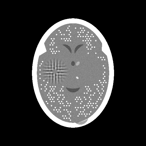
Figure 6: Mathematical phantom used in the simulated experiments. Image range is $[0,1]$.

A parallel version of GALE, called GALEP, was also tested to see how the algorithm scales in multiprocessing environments. All algorithms were executed in a quad core i7 7700HQ processor with 32GB of RAM. GALEP used four threads of processing. GALE and GALEP were implemented in C/C++ with the FFTW3 library [22] used for FFT computations.

For measures of approximation quality, we used the following: Given a $\boldsymbol{y}\in\mathbb{C}^{MN}$ such that $y_{I,J}\neq 0$ for all $(I,J)\in\{0,1,\dots,M-1\}\times\{0,1,\dots,N-1\}$ and an approximation $\overline{\boldsymbol{y}}$ to $\boldsymbol{y}$,

1. the Mean Relative Error (MRE) is defined as

   $$\text{MRE}\left(\boldsymbol{y},\overline{\boldsymbol{y}}\right):=\frac{1}{MN}\sum_{I=0}^{M-1}\sum_{J=0}^{N-1}\frac{\left|y_{I,J}-\overline{y}_{I,J}\right|}{\left|y_{I,J}\right|};$$

2. the Relative Squared Error (RSE) is defined as

   $$RSE\left(\boldsymbol{y},\overline{\boldsymbol{y}}\right):=\frac{\sum_{I=0}^{M-1}\sum_{J=0}^{N-1}\left|y_{I,J}-\overline{y}_{I,J}\right|^{2}}{\sum_{I=0}^{M-1}\sum_{J=0}^{N-1}\left|y_{I,J}\right|^{2}}.$$

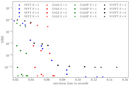
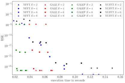
Figure 7: MREs (left) and RSEs (right) between the DFT over the GALFD computed using (1) and the approximation obtained by various schemes. For a given algorithm and for a given value of the parameter $S$, the marker for the points representing results with different values of $P$ was kept the same, but these can be differentiated by its computation time: the larger the $P\in\{768,1024,1280\}$, the longer a given algorithm with a given value of $S$ takes to run to completion.

The results are shown in Figure 7, where an advantage of the GALE is seen over the NFFT and the NUFFT. It is clear that if an MRE below $10^{-7}$ desired, then, within a same amount of computation time, it is possible to obtain a better approximation for the DFT over the GALFD with GALE than with the NFFT or of the NUFFT. This is so because the $O\left(m^{2}S\right)$ term in the flops count for GALE becomes significantly smaller than the $O\left(m^{2}S^{2}\right)$ term in the NFFT’s (and NUFFT’s) flops count. In fact, the $O\left(m^{2}S^{2}\right)$ term dominates (17) because increasing $S$ has a larger impact on NFFT’s running time than increasing $P$, whereas the opposite is true for GALE.

Notice that the relative gains are significant. For example, for an RSE of around $10^{-26}$, GALE takes half of the time of NFFT to complete the computations. Furthermore, although the computation times seem small, in MRI applications one usually deals with multiple channel data, volumetric images, and several different contrasts in, e.g., quantitative imaging. This means that computation times add up and therefore efficient numerical techniques for the computation of the DTFT over radial domains can have important practical consequences, especially when iterative reconstruction methods, as discussed in D, are used to recover the $\boldsymbol{x}$ in (1) from the observed data, indicated by the left-hand-side of (1).

We also notice that GALE scales well in multiprocessing environments. A parallel CPU implementation of the NFFT (but not of the NUFFT) is publicly available and recent research indicates that careful domain-specific implementations of the NUFFT can be competitive in GPU environments [23], however, extensive software comparisons in parallel environments are out of the scope of the present paper and we do not further pursue this topic here. A worth-mentioning alternative that could be adapted to the sampling circumstances that we are considering can be found in [24].

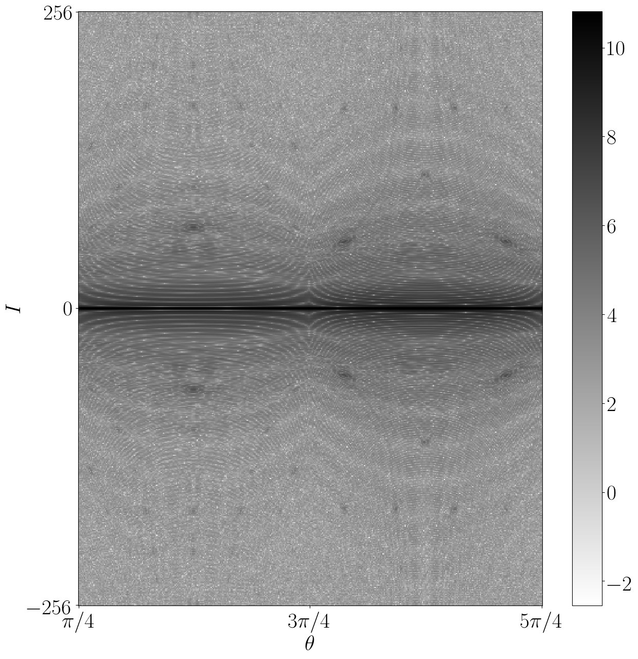
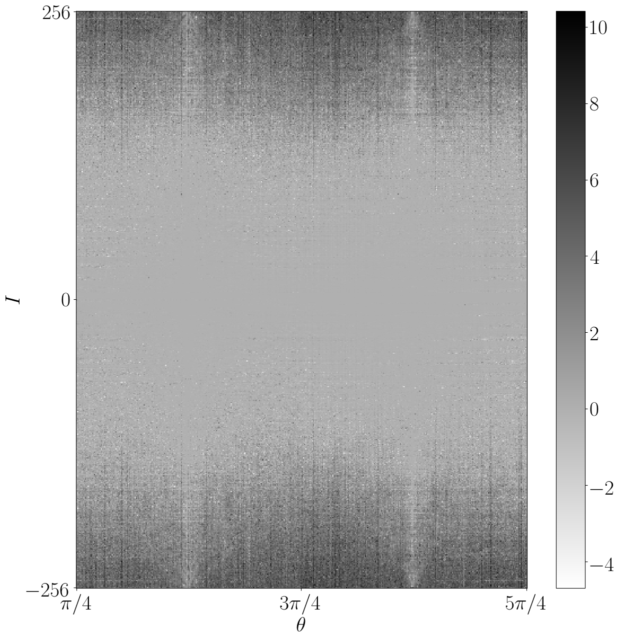
Figure 8: Left: Image of $\log\left|y_{I,J}\right|$ where $\boldsymbol{y}=\mathcal{D}_{\mathfrak{N}_{500,400}}\boldsymbol{x}$. It can be seen that the largest values are highly concentrated around the region $|I|\approx 0$. Right: Image of $\log\frac{\left|\tilde{y}_{I,J}-y_{I,J}\right|}{\left|\overline{y}_{I,J}-y_{I,J}\right|}$, where $\tilde{\boldsymbol{y}}$ is the approximation obtained by GALE with $(P,S)=(768,6)$ and $\overline{\boldsymbol{y}}$ is the approximation obtained by GALE with $(P,S)=(1280,6)$. Note that the accuracy improvements obtained by a larger Fourier oversampling occur mainly in the region $|I|\gg 0$. In both images, each column represents one ray of the GALFD.

An interesting observation regarding these experiments is that if absolute, rather than relative, errors are considered, then increasing the Fourier oversampling parameter $P$ has little effect on the approximation error for GALE. The explanation is given by the combination of two reasons: (i) the nature of the approximation error bound (12), which, as depicted in Figure 5, is such that, for GALE, the Fourier oversampling is only important in the higher frequencies components of the Fourier domain and (ii) the fact that medical images in general, and our phantom in particular, have most of their energy concentrated in the low frequency parts of the Fourier domain. Figure 8 illustrates these two points. On the left, we can see that indeed the largest values of the DTFT of the phantom are very concentrated in the region $|I|\approx 0$. On the right, we observe that increasing the Fourier sampling parameter does provide significantly better accuracy, but this improvement happens mostly in the region $|I|\gg 0$.

Realizing that the NUFFT does not achieve the same level of accuracy as the other two techniques, we have devised an experiment to further investigate this phenomenon. We have considered the function

$$f(\boldsymbol{x})=\left\|\mathrm{D}_{\mathfrak{N}_{512,400}}\boldsymbol{x}-\boldsymbol{y}\right\|^{2},$$

where, again, $\boldsymbol{y}$ is as given in (18) and is computed directly from the definition (1). We have then run $20$ iterations of the Conjugate Gradient (CG) method for the minimization of this function. We have performed two different reconstructions, one using GALE and the other using the NUFFT with parameters $S=2$ for both methods and $P=768$ for the NUFFT and $P=520$ for the GALE to approximate $\mathrm{D}_{\mathfrak{N}_{512,400}}$ and its adjoint. The parameter values were such that the computation time was approximately the same for both algorithms.

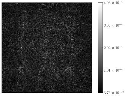
Figure 9: Images of the errors $\left|x_{i,j}^{\dagger}-x_{i,j}^{20}\right|$, where $\boldsymbol{x}^{20}$ is iteration $20$ of the CG method started with $\boldsymbol{x}^{0}=\boldsymbol{x}^{\dagger}$ as detailed in Subsection 4.1. Left: Errors obtained using the NUFFT with $S=2$ and $P=768$ for approximating $\mathrm{D}_{\mathfrak{N}_{512,400}}$ and its adjoint. The maximum error is $1.8\cdot 10^{-3}$. Right: Errors obtained using the GALE with $S=2$ and $P=520$ for approximating $\mathrm{D}_{\mathfrak{N}_{512,400}}$and its adjoint. The maximum error is $4.0\cdot 10^{-4}$.

Differences between the reconstructed images and the image $\boldsymbol{x}^{\dagger}$ that originated the data are possibly caused by the following:

1. Finite termination of the iterative method;

2. Infinite number of solutions for the problem due to number of equations smaller than the number of variables;

3. Approximation errors of the methods.

Notice that although the system matrix in this case might not be positive definite, only the last item will be different between experiments using GALE and experiments using the NUFFT, so, in order to be able to assess the influence of the last item alone, the CG algorithm was started with the actual desired image $\boldsymbol{x}^{\dagger}$ and therefore the method should not move from the starting point if computations were performed with full numerical accuracy. The resulting images of the differences between reconstructed and original images can be seen in Figure 9 and show an interesting phenomenon: the image obtained by the NUFFT presents a very structured error, whereas the image obtained using the GALE has a random-like error. In unreported experiments, we have increased the Fourier oversampling and the truncation parameter for the NUFFT, and we were able to rule out circular interference as the sole cause of the observed structure. Although the magnitude of the error can indeed be reduced this way, it always presents some sort of structure that follows the reconstructed image.

4.2 Magnetic Resonance Image Reconstruction

This subsection is dedicated to experiments involving image reconstruction in magnetic resonance. In MRI, the data acquisition process provides a signal that corresponds to the CFT of the object, modulated by the receiver sensitivities. More precisely, the image is assumed to be an absolutely integrable complex-valued function in the plane $f:\mathbb{R}^{2}\to\mathbb{C}$ and the data are assumed to take the form

$$y_{I,J}^{c}\approx\widehat{\zeta_{c}f}(\xi_{I,J},\upsilon_{I,J} )=\int_{\mathbb{R}^{2}}\zeta_{c}(\boldsymbol{z})f(\boldsymbol{z})e^{-\imath\left(z_{1}\xi_{I,J}+z_{2}\upsilon_{I,J}\right)}\mathrm{d}\boldsymbol{z},$$

$$(I,J,c)\in\{0,1,\dots,M-1\}\times\{0,1,\dots,N-1\}\times\{0,1,\dots,C-1\},$$

where each bounded function $\zeta_{c}:\mathbb{R}^{2}\to\mathbb{C}$ is the sensitivity function of receive coil $c$. In our case, we acquired data with

$$\left\{\left(\xi_{I,J},\upsilon_{I,J}\right):(I,J)\in\{0,1,\dots,M-1\}\times\{0,1,\dots,N-1\}\right\}=\mathfrak{N}_{M,N}.$$

Moreover, we can assume that

$$f=\sqrt{\sum_{c=0}^{C-1}\left(\zeta_{c}f\right)^{2}}.$$

The radial nature of the GALFD allows us to take an interesting analytical approach to image reconstruction from this kind of dataset, using a tool from CT [13, 14, 25], which is the Filtered Backprojection (FBP) algorithm. Let us assume that $f\in\mathscr{S}(\mathbb{R}^{2})$, where $\mathscr{S}(\mathbb{R}^{2})$ is the Schwartz space [14], then

$$f=\mathcal{B}\circ\mathcal{W}\circ\mathcal{R}[f],$$

where $\mathcal{R}$ is the Radon Transform (RT)

$$\mathcal{R}[f](\theta,t):=\int_{\mathbb{R}}f\left(s\left(-\sin\theta,\cos\theta\right)+t\left(\cos\theta,\sin\theta\right)\right)\mathrm{d}s,$$

$\mathcal{B}$ is the Backprojection operator

$$\mathcal{B}[g](\boldsymbol{z}):=\int_{[0,\pi]}g(\theta,z_{1}\cos\theta+z_{2}\sin\theta)\mathrm{d}\theta,$$

which turns out to be the adjoint of the Radon Transform $\mathcal{B}=\mathcal{R}^{*}$, and $\mathcal{W}$ has the form

$$\mathcal{W}=\mathcal{E}^{-1}\circ\mathcal{C}\circ\mathcal{E},$$

where $\mathcal{E}$ is an operator that computes the one-dimensional Fourier Transform with relation to the second variable of a function of two variables

$$\mathcal{E}[g](\theta,\omega):=\int_{\mathbb{R}}g(\theta,t)e^{-\imath\omega t}\mathrm{d}t,$$

which in turn means that $\mathcal{E}^{-1}=(2\pi)^{-1}\mathcal{E}^{*}$, and $\mathcal{C}$ is a diagonal operator of the form

$$\mathcal{C}[g](\theta,\omega):=|\omega|g(\theta,\omega).$$

Therefore, denoting $\mathcal{G}:=\mathcal{E}\circ\mathcal{R}$ we have

$$f=\frac{1}{2\pi}\mathcal{G}^{*}\circ\mathcal{C}\circ\mathcal{G}[f].$$ (19)

(For other interesting and relevant inversion techniques see [26, 27, 28].) Notice that operator $\mathcal{C}$ can be described as pointwise multiplication by a Density Compensation Function (DCF) $h(\omega,\theta)=|\omega|$ and that, because of the radial nature of the GALFD, we can write $(\xi_{I,j},\upsilon_{I,J})=\left(\omega_{I}\cos\theta_{J},\omega_{I}\sin\theta_{J}\right)$, where $\left|\omega_{I}\right|=\sqrt{\xi_{I,J}^{2}+\upsilon_{I,J}^{2}}$. Now, we consider the Fourier Slice Theorem (FST) [13, 14, 25], which states that

$$\mathcal{G}[f](\theta,\omega)=\mathcal{F}[f](\omega\cos\theta,\omega\sin\theta),$$

and then we approximate the above integral model by a discrete one.

Assume that $\boldsymbol{x}^{c}\in\mathbb{C}^{mn}$ is such that $x_{i,j}^{c}=f_{c}(j-\nicefrac{{n}}{{2}},i-\nicefrac{{m}}{{2}})$, where we denoted $f_{c}:=\zeta_{c}f$, then we have, using the FST and then approximating the integrations by a sum,

$$y_{I,J}^{c} {}=\mathcal{G}[f_{c}]\left(\theta_{I},\omega_{J}\right)=\mathcal{F}\left[f_{c}\right]\left(\omega_{I}\cos\theta_{J},\omega_{I}\sin\theta_{J}\right)$$

$${}\approx\frac{1}{mn}\sum_{i=0}^{m-1}\sum_{j=0}^{n-1}x_{i,j}^{c}e^{-\imath\left((j-\nicefrac{{n}}{{2}})\xi_{I,J}+(i-\nicefrac{{m}}{{2}})\upsilon_{I,J}\right)}$$

$${}=\frac{e^{\imath\left((\nicefrac{{n}}{{2}})\xi_{I,J}+(\nicefrac{{m}}{{2}})\upsilon_{I,J}\right)}}{mn}\sum_{i=0}^{m-1}\sum_{j=0}^{n-1}x_{i,j}^{c}e^{-\imath\left(j\xi_{I,J}+i\upsilon_{I,J}\right)}.$$

That is,

$$\boldsymbol{y}^{c}\approx\mathrm{Z}\mathrm{D}_{\mathfrak{N}_{M,N}}\boldsymbol{x}^{c},$$

where the diagonal linear operator $\mathrm{Z}:\mathbb{C}^{MN}\to\mathbb{C}^{MN}$ is given componentwise by

$$(\mathrm{Z}\boldsymbol{y})_{I,J}=y_{I,J}\frac{e^{\imath\left((\nicefrac{{n}}{{2}})\xi_{I,J}+(\nicefrac{{m}}{{2}})\upsilon_{I,J}\right)}}{mn}.$$

In other words, the composite operator $\mathrm{Z}\mathrm{D}_{\mathfrak{N}_{M,N}}$ serves as a discrete approximation for $\mathcal{G}[f_{c}]$ when the latter is computed over $(\xi,\theta)\in\mathfrak{N}_{M,N}$.

The validity of the discretization discussed above depends on bandwidth considerations about the functions $f_{c}$. An in-depth discussion about this subject can be found in [14], but for us, the practical value of this approach is that it allows us to make use of a discrete version of (19) that reads

$$\boldsymbol{x}^{c}\approx\mathrm{D}_{\mathfrak{N}_{M,N}}^{*}\mathrm{Z^{*}}\mathrm{C}\mathrm{Z}\mathrm{D}_{\mathfrak{N}_{M,N}}\boldsymbol{x}^{c},$$

where the diagonal linear operator $\mathrm{C}:\mathbb{C}^{MN}\to\mathbb{C}^{MN}$ is given componentwise by

$$(\mathrm{C}\boldsymbol{y})_{I,J}=y_{I,J}\sqrt{\xi_{I,J}^{2}+\upsilon_{I,J}^{2}}.$$

Finally, the algorithm for inverting the MR data consists of computing

$$\boldsymbol{x}^{c}=\mathrm{D}_{\mathfrak{N}_{M,N}}^{*}\mathrm{Z^{*}}\mathrm{C}\boldsymbol{y}^{c},\quad c\in\{0,1,\dots,C-1\}$$

and then

$$x_{i,j}=\sqrt{\sum_{c=0}^{C-1}\left(x_{i,j}^{c}\right)^{2}},\quad(i,j)\in\{0,1,\dots,m-1\}\times\{0,1,\dots,n-1\}.$$

The above algorithm was applied to the MRI reconstruction of a physical phantom and of a human brain, where image dimensions were $m=n=512$ ($256$ pixels with twofold oversampling, i.e., data were acquired for an ROI twice as large as the one that was known to contain the object in order to avoid circular interference) and data dimensions were $M=512$, $N=400$ and $C=20$ for the phantom, and $N=800$ and $C=16$ for the brain (recall that the data were collected in $M$ samples for each of the $N$ rays and each sample is measured in parallel by $C$ coils). Two-dimensional Fourier data were obtained by applying the IFFT along the $z$ direction of MRI data acquired using a stack-of-stars 3D Gradient-Recalled Echo (GRE) linogram sequence with golden-angle ordering at $3$ Tesla. We used two different ways of computing the adjoint operator $\mathrm{D}_{\mathfrak{N}_{M,N}}^{*}$. Besides GALE, the NUFFT [15] adjoint routine was tested for comparison. We used $S=3$ and $P=768$ for both the NUFFT and GALE. GALE was used with $8$ threads of execution. For these experiments, a MATLAB binding was created for GALE in order to have it running in the same environment as the NUFFT package, which is implemented in MATLAB.

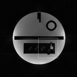
Figure 10: Reconstruction of physical phantom image from magnetic resonance data. Left: Using GALE ($0.025$ seconds of computation per coil per slice). Right: Using NUFFT within ($0.034$ seconds of computation per coil per slice). Top: Full image reconstructions. Bottom: Enlarged detail of small reconstructed structures (from regions delimited by dotted lines in top row).

Figure 11: Reconstruction of human brain image from magnetic resonance data. Left: Using GALE ($0.028$ seconds of computation per coil per slice). Right: Using NUFFT ($0.063$ seconds of computation per coil per slice). Top: Full image reconstructions. Bottom: Enlarged detail of small reconstructed structures (from regions delimited by dotted lines in top row).

The resulting images from the GALE and from the NUFFT are visually indistinguishable in the two experiments, as can be seen in Figures 10 and 11, with the existing numerical differences being irrelevant for human visualization. Furthermore, the good image quality indicates that the GALFD is a sound way of sampling the Fourier space in MRI and that the proposed numerical approach is useful in practical scenarios, potentially leading to a significant reduction in computation time without loss of accuracy when compared to other available algorithms for the same task.

5 Conclusions

We introduced a new family of subsets, each of which is called a GALFD, of the two-dimensional Fourier space, that has desirable properties for MRI reconstruction applications. The paper was dedicated to the study of GALE, a new approach for the numerical computation of the DFT over finite domains, in particular over a GALFD. GALE was demonstrated to be fast and accurate when compared to existing techniques available for the task. Therefore, among the desirable practical features of GALE is its good accuracy/computation time trade-off. An upper bound on the approximation error incurred by GALE was provided; it can be used to gain insight on how to select the method’s parameters in practical settings.

Generalizing the GALFD sampling scheme to a 3D configuration is planned for future work, again with application to MRI as the main goal [29]. In this case, the computation time reductions of a linogram-based approach is even more significant, because an appropriate selection of the rays in 3D space allows the method to use a summation of $O(S)$ terms, while some current methods use $O\left(S^{3}\right)$ terms for this case, which in practice precludes the use of three-dimensional radial sampling of the Fourier space.

Appendix A The 1D Discrete Fourier Transform

The 1D DFT of a vector $\boldsymbol{x}\in\mathbb{C}^{m}$ is given by:

$$\hat{x}_{I}:=\sum_{i=0}^{m-1}x_{i}e^{-\imath i\frac{2\pi I}{m}},\quad I\in\{0,1,\dots,m-1\}.$$

This defines a linear operator $\mathrm{F}_{m}:\mathbb{C}^{m}\rightarrow\mathbb{C}^{m}$ such that $\hat{\boldsymbol{x}}=\mathrm{F}_{m}\boldsymbol{x}$ is given componentwise as above. It is possible to perform the computation of $\mathrm{F}_{m}\boldsymbol{x}$ efficiently with an FFT of length $m$ that uses roughly $5m\log_{2}m$ flops. Inversion of the 1D DFT is simple:

$$x_{i}=\frac{1}{m}\sum_{I=0}^{m-1}\hat{x}_{I}e^{\imath I\frac{2\pi i}{m}},\quad i\in\{0,1,\dots,m-1\}.$$

Such a computation is performed efficiently by the Inverse FFT (IFFT) algorithm that uses about as many flops as the FFT does. We denote this inverse operator by $\mathrm{F}_{m}^{-1}:\mathbb{C}^{m}\rightarrow\mathbb{C}^{m}$.

There are times when we wish to compute, for some $M\geq m$,

$$\hat{x}_{I}:=\sum_{i=0}^{m-1}x_{i}e^{-\imath i\frac{2\pi I}{M}},\quad I\in\{0,1,\dots,M-1\}.$$ (20)

Such a computation provides a finer sampling of the Fourier space and can be obtained by computing $\mathrm{F}_{M}\mathrm{Z}_{m,M}\boldsymbol{x}$, where $\mathrm{Z}_{m,M}:\mathbb{C}^{m}\rightarrow\mathbb{C}^{M}$ is the zero-padding operator given by

$$(\mathrm{Z}_{m,M}\boldsymbol{x})_{i}:=\left\{\begin{array}[]{ll}x_{i},&\quad\text{if}\quad 0\leq i<m-1,\\ 0,&\quad\text{if}\quad m\leq i<M.\end{array}\right.$$

It is helpful to use the notation $\text{FFT}(\boldsymbol{x},m,M):=\mathrm{F}_{M}\mathrm{Z}_{m,M}\boldsymbol{x}$, which also implies that such a computation is done using the FFT algorithm of length $M$ after zero-padding the vector $\boldsymbol{x}\in\mathbb{R}^{m}$, where $m\leq M$. Correspondingly, for $\boldsymbol{x}\in\mathbb{C}^{M}$ with $M\geq m$, we denote $\text{IFFT}(\boldsymbol{x},m,M):=\mathrm{T}_{m,M}\mathrm{F}_{M}^{-1}\boldsymbol{x}$, where $\mathrm{T}_{m,M}:\mathbb{C}^{M}\rightarrow\mathbb{C}^{m}$ is the truncation operator defined componentwise as $\left(\mathrm{T}_{m,M}\boldsymbol{x}\right)_{i}=x_{i}$, $i\in\{0,1,\dots m-1\}$. Note that $\mathrm{T}_{m,M}\mathrm{F}_{M}^{-1}=\nicefrac{{1}}{{M}}(\mathrm{F}_{M}\mathrm{Z}_{m,M})^{*}$.

Also useful for us is to notice that the range $I\in\{0,1,\dots,M-1\}$ in (20) can be changed very easily to, say, $I\in\{-R,-R+1,\dots,-R+M-1\}$ by computing

$$\sum_{i=0}^{m-1}x_{i}e^{-\imath i\frac{2\pi(I-R)}{M}}=\sum_{i=0}^{m-1}x_{i}e^{\imath i\frac{2\pi R}{M}}e^{-\imath i\frac{2\pi I}{M}},\quad I\in\{0,1,\dots,M-1\},$$

that is multiplying each component $x_{i}$ of $\boldsymbol{x}\in\mathbb{R}^{m}$ by $e^{\imath i\frac{2\pi R}{M}}$ before computing $\text{FFT}(\boldsymbol{x},m,M)$.

Appendix B The Chirp-Z Transform

Let $\alpha\in\mathbb{R}$, $R\in\mathbb{Z}$, and $m$, $M$, $P$ be positive integers such that $P\geq m$. Consider the linear operator $\mathrm{F}_{m}^{\alpha,M,P,R}:\mathbb{C}^{m}\rightarrow\mathbb{C}^{P}$ such that, for $\boldsymbol{x}\in\mathbb{C}^{m}$, if $\hat{\boldsymbol{x}}^{\alpha,M,P,R}=\mathrm{F}_{m}^{\alpha,M,P,R}\boldsymbol{x}$, then $\hat{\boldsymbol{x}}^{\alpha,M,P,R}\in\mathbb{C}^{P}$ is given componentwise by

$$\hat{x}_{I}^{\alpha,M,P,R}:=\sum_{i=0}^{m-1}x_{i}e^{-\imath i\frac{2\pi(I-R)}{M}\alpha}=\sum_{i=0}^{m-1}x_{i}e^{\imath i\frac{2\pi R}{M}\alpha}e^{-\imath i\frac{2\pi I}{M}\alpha},\quad I\in\{0,1,\dots,P-1\}.$$ (21)

We call the $\hat{\boldsymbol{x}}^{\alpha,M,P,R}\in\mathbb{C}^{P}$ thus obtained the Chirp-Z Transform of $\boldsymbol{x}\in\mathbb{C}^{m}$. There is an efficient equivalent way of performing this computation, for which a key observation is that

$$\hat{x}_{I}^{\alpha,M,P,R} {}=\sum_{i=0}^{m-1}x_{i}e^{\imath i\frac{2\pi R}{M}\alpha}e^{-\imath\frac{\pi\alpha}{M}\left(I^{2}+i^{2}-(I-i)^{2}\right)}$$ (22)

$${}=e^{-\imath\frac{\pi\alpha}{M}I^{2}}\sum_{i=0}^{m-1}x_{i}e^{\imath i\frac{2\pi R}{M}\alpha}e^{-\imath\frac{\pi\alpha}{M}i^{2}}e^{\imath\frac{\pi\alpha}{M}(I-i)^{2}}.$$

We will return to this computation shortly; meanwhile we consider another useful concept.

A circular convolution $\boldsymbol{p}\circledast\boldsymbol{q}\in\mathbb{C}^{Q}$ between two vectors $\boldsymbol{p}\in\mathbb{C}^{Q}$ and $\boldsymbol{q}\in\mathbb{C}^{Q}$ is defined by

$$(\boldsymbol{p}\circledast\boldsymbol{q})_{I}:=\sum_{i=0}^{Q-1}p_{i}q_{(I-i)\%Q},\quad I\in\{0,1,\dots,Q-1\},$$ (23)

The easily proven Circular Convolution Theorem (CCT) states that

$$\boldsymbol{p}\circledast\boldsymbol{q}=F_{Q}^{-1}\left((F_{Q}\boldsymbol{p})\odot(F_{Q}\boldsymbol{q})\right),$$ (24)

where $\boldsymbol{u}\odot\boldsymbol{v}\in\mathbb{C}^{Q}$ is obtained by componentwise multiplication of $\boldsymbol{u}\in\mathbb{C}^{Q}$ and $\boldsymbol{v}\in\mathbb{C}^{Q}$.

The CCT provides efficient computation of a circular convolution using the FFT and the IFFT. We notice that the summation on the right-hand side of (22) can obtained as part of a computation of the form (23). To be precise, let $Q=2P$ and $\boldsymbol{p}\in\mathbb{C}^{Q}$, $\boldsymbol{q}\in\mathbb{C}^{Q}$ be given by

$$p_{i}=\left\{\begin{array}[]{ll}x_{i}e^{-\imath i\frac{\pi\alpha}{M}(i-2R)},&\quad\text{if}\quad 0\leq i<m,\\ 0,&\quad\text{if}\quad m\leq i<Q,\end{array}\right.$$ (25)

$$q_{i}=\left\{\begin{array}[]{ll}e^{\imath\frac{\pi\alpha}{M}i^{2}},&\quad\text{if}\quad 0\leq i<P,\\ e^{\imath\frac{\pi\alpha}{M}(Q-i)^{2}},&\quad\text{if}\quad P\leq i<Q.\end{array}\right.$$ (26)

Then, we have

$$\hat{x}_{I}^{\alpha,M,P,R}=e^{-\imath\frac{\pi\alpha}{M}I^{2}}(\boldsymbol{p}\circledast\boldsymbol{q})_{I},\quad I\in\{0,1,\dots,P-1\}.$$ (27)

Now we give an efficient algorithm for the computation of the CZT. Since CZTs with fixed parameters $m$, $\alpha$, $M$, $P$, and $R$ are often computed for several inputs, it is convenient to reuse all data-independent computations. This is why we separate initialization, which is performed by Algorithm 3, from the data-dependent calculations executed by Algorithm 4, which makes use of the parameters initialized by Algorithm 3 while computing the CZT itself.

Algorithm 3 $\text{CZT-I}(m,\alpha,M,P,R)$

1:  for $i\in\{0,1,\dots,m-1\}$ do

2:        $r_{i}\leftarrow e^{-\imath i\frac{\pi\alpha}{M}(i-2R)}$

3:  for $i\in\{0,1,\dots,2P-1\}$ do

4:        $q_{i}\leftarrow\left\{\begin{array}[]{ll}e^{\imath\frac{\pi\alpha}{M}i^{2}},&\quad\text{if}\quad 0\leq i<P,\\ e^{\imath\frac{\pi\alpha}{M}(2P-i)^{2}},&\quad\text{if}\quad P\leq i<2P.\end{array}\right.$

5:  $\hat{\boldsymbol{q}}\leftarrow\text{FFT}(\boldsymbol{q},2P,2P)$

6:  for $I\in\{0,1,\dots,P-1\}$ do

7:        $s_{I}\leftarrow e^{-\imath\frac{\pi\alpha}{M}I^{2}}$

8:  return $(\hat{\boldsymbol{q}},\boldsymbol{r},\boldsymbol{s})$

Algorithm 4 $\text{CZT}(\boldsymbol{x},m,P,\hat{\boldsymbol{q}},\boldsymbol{r},\boldsymbol{s})$

1:  for $i\in\{0,1,\dots,m-1\}$ do

2:        $p_{i}\leftarrow x_{i}r_{i}$

3:  $\hat{\boldsymbol{p}}\leftarrow\text{FFT}(\boldsymbol{p},m,2P)$

4:  for $I\in\{0,1,\dots,2P-1\}$ do

5:        $\hat{p_{I}}\leftarrow\hat{p_{I}}\hat{q}_{I}$

6:  $\boldsymbol{y}\leftarrow IFFT(\hat{\boldsymbol{p}},P,2P)$

7:  for $I\in\{0,1,\dots,P-1\}$ do

8:        $y_{I}\leftarrow y_{I}s_{I}$

9:  return $(\boldsymbol{y})$

Finally, let us relate Algorithm 4 with the desired computation (21). We assume that we have computed $(\hat{\boldsymbol{q}},\boldsymbol{r},\boldsymbol{s})\leftarrow\text{CZT-I}(m,\alpha,M,P,R)$ and then analyze the output of $(\boldsymbol{y})\leftarrow\text{CZT}(\boldsymbol{x},m,P,\hat{\boldsymbol{q}},\boldsymbol{r},\boldsymbol{s})$. First we notice that after Steps 1-2 of Algorithm 4, because $\boldsymbol{r}$ was computed in Steps 1-2 of Algorithm 3, we have $p_{i}=x_{i}e^{-\imath i\frac{\pi\alpha}{M}(i-2R)}$ for $i\in\{0,1,\dots,m-1\}$. Then, after Step 3 of Algorithm 4, $\hat{\boldsymbol{p}}$ will hold exactly the 1D DFT of the sequence defined in (25). Because $\hat{\boldsymbol{q}}$ was computed in Steps 3-5 of Algorithm 3, we know that it holds the 1D DFT of the sequence defined in (26). Thus, due to the CCT (24), we know that Steps 4-6 of Algorithm 4 give $y_{I}=(\boldsymbol{p}\circledast\boldsymbol{q})_{I}$ for $I\in\{0,1,\dots,P-1\}$. Steps 7-8 of Algorithm 4 complete the computation of (21) through the equivalent formulation (27) with the use of (24).

Appendix C Relevance to Practical MRI in Medicine

Our desire to pursue the concept of GALFD for practical imaging applications is driven by the recent advances in the use of radial imaging approaches for MRI, with various sorts of polar-type sampling of the Fourier space. Radial imaging has shown advantages for cardiac [30] and abdominal [4] imaging, as well as short-T2 [31] and sodium imaging [32]. While polar sampling with projection-reconstruction was one of the original methods used for MRI, it had been mostly abandoned for many years in favor of the mathematically simpler and often more robust imaging methods that use direct Cartesian grid sampling of the Fourier space; see Figure 1. Linogram (“concentric squares”) data sampling approaches to radial imaging (as in Figure 2, left) were demonstrated early on to have computational advantages over the more common “concentric circles” polar sampling schemes (as in Figure 1, right). This is due to linogram sampling enabling the use of direct Fourier reconstruction methods without the need for the time-consuming and resolution-degrading intermediate interpolation steps used with reconstruction from samples on concentric circles. However, this advantage was not compelling enough to lead to their widespread adoption at that time, for the relatively limited size data sets that were being acquired then. The principal advantage of radial data sampling approaches for magnetic resonance imaging is that it permits the use of very short delays before acquiring the data, which is important for imaging of short-T2 species of signal sources [31], such as hydrogen in large molecules (such as collagen or myelin) or sodium [32]. In this case, the computational advantages of linogram imaging approaches over conventional polar sampling methods become particularly important for acquisition and reconstruction of fully 3D radial data sets. The limitations of conventional polar radial image reconstruction methods has led to the common use of “stack-of-stars” data acquisition approaches (“concentric cylinders”) for 3D radial imaging, with their longer associated data acquisition delay times, rather than fully 3D radial sampling; using linogram 3D approaches (“concentric cubes” [29]) thus has the potential for significantly improved (shorter) delays in the data acquisition times, as compared to the conventional approach.

Another factor leading to the recently renewed interest in the radial sampling MRI methods has been their use for imaging of dynamic processes, such as contrast enhancement dynamics [4], or of moving objects, such as the heart. In this case, we typically use golden angle incrementation of the orientation of the consecutively acquired radial sample sets, which permits continuous data acquisition with the ability for flexible rebinning of the data for use in the image reconstruction, with approximately uniform angular distributions of the samples in each such set [30] . However, this still requires the time-consuming interpolation steps for reconstruction, with its associated disadvantages for conventional 2D imaging, and it has again led to the conventional use of the “stack-of-stars” approach for 3D imaging with golden angle increments, rather than fully 3D radial imaging acquisitions. The use of modified linogram approaches with golden angle increments, as demonstrated in the present work, allows for the use of direct Fourier approaches for at least one dimension of the image reconstruction, rather than needing to rely on intermediate interpolations for all dimensions, with the associated advantages of computational speed and precision, and thus can potentially enable improved performance for MRI in these kinds of applications. This is likely to be particularly useful for 3D imaging.

Appendix D Iterative Algorithms

Several practical circumstances require data acquisition in CT or MRI to be done in a less than ideal manner leading to increased noise and/or small number of data samples. Examples include imaging of moving objects, requirements of radiation exposure reduction in CT, sodium imaging in MRI, etc.

In such cases, methods that provide the best reconstructions usually work by successively refining an initial estimate of the desired image, that is, they are iterative. A reason why such methods are powerful is their capability of solving optimization models of image reconstruction, but quite a few efficacious iterative methods do not rely on an optimization model. Many iterative methods share a common structure that we now discuss for the problem of recovering an $\boldsymbol{x}\in\mathbb{C}^{mn}$ in (1) from experimentally obtained vector $\boldsymbol{y}$ of the values $\mathcal{D}[\boldsymbol{x}](\xi,\upsilon)$ of the DTFT of $\boldsymbol{x}$ for all $(\xi,\upsilon)\in\mathfrak{D}$, with $\mathfrak{D}$ a GALFD.

Such an iterative method starts with some $\boldsymbol{x}^{0}\in\mathbb{C}^{mn}$ and proceeds by successive application of an algorithmic operator $\mathcal{A}$ to the current iterate $\boldsymbol{x}^{k}$ to obtain the next one: $\boldsymbol{x}^{k+1}=\mathcal{A}(\boldsymbol{x}^{k})$, $k=0,1,2,\dots$. It is in the computation of $\mathcal{A}(\boldsymbol{x}^{k})$ that GALE can be efficacious. To demonstrate this, we refer to [13, Section 12.2] that discusses in detail a particular iterative method of CT reconstruction. For example, Equation (12.25) there can be rewritten in the notation of our current paper as

$$\boldsymbol{x}^{k+1}=\mathbf{x}^{k}+\lambda^{k}\left(r^{2}\mathcal{O}^{*}\left(\boldsymbol{y}-\mathcal{O}\boldsymbol{x}^{k}\right)+\left(\mu_{X}-\boldsymbol{x}^{k}\right)\right),$$ (28)

where $\mathcal{O}$ is the operator calculated by Algorithm 2 (GALE) and $\mathcal{O}^{*}$ is its adjoint, $\lambda^{k}$ is a real number (the relaxation parameter in the $k$th iteration), $r$ is a real number (the signal-to-noise ratio in the data collection) and $\mu_{X}$ is the expected prior value of $\boldsymbol{x}$. If data were acquired in a GALFD, then GALE could be used for efficient computations of $\mathcal{O}\boldsymbol{x}^{k}$ and of $\mathcal{O}^{*}\left(\boldsymbol{y}-\mathcal{O}\boldsymbol{x}^{k}\right)$, which are often the most time consuming operations of each iteration. This would lead to substantial computational savings that could bring such iterative reconstruction techniques closer to clinical practice.

References

References

- [1] Winkelmann S, Schaeffter T, Koehler T, Eggers H and Doessel O 2006 IEEE Transactions on Medical Imaging 26 68–76
- [2] Benkert T, Tian Y, Huang C, DiBella E V R, Chandarana H and Feng L 2018 Magnetic Resonance in Medicine 80 286–293
- [3] Castets C R, Cois W L, Wecker D, Ribot E J, Trotier A J, Thiaudière E, Franconi J M and Miraux S 2017 Magnetic Resonance in Medicine 77 1831–1840
- [4] Feng L, Grimm R, Block K T, Chandarana H, Kim S, Xu J, Axel L, Sodickson D K and Otazo R 2014 Magnetic Resonance in Medicine 72 707–717
- [5] Edholm P R and Herman G T 1987 IEEE Transactions on Medical Imaging 6 301–307
- [6] Edholm P R, Herman G T and Roberts D A 1988 IEEE Transactions on Medical Imaging 7 239–246
- [7] Axel L, Herman G T, Roberts D A and Dougherty L 1990 IEEE Transactions on Medical Imaging 9 447–449
- [8] Ersoza A and Muftuler L T 2016 NMR in Biomedicine 29 240–248
- [9] Yang Y, Liu F, Li M, Jin J, Weber E, Liu Q, and Crozier S 2017 IEEE Transactions on Biomedical Engineering 64 816–825
- [10] Cooley J W and Tukey J W 1965 Mathematics of Computation 19 297–301
- [11] Block K T, Uecker M and Frahm J 2007 Magnetic Resonance in Medicine 57 1086–1098
- [12] Yeh E N, Stuber M, McKenzie C A, Botnar R M, Leiner T, Ohliger M A, Grant A K, Willig-Onwuachi J D and Sodickson D K 2005 Magnetic Resonance in Medicine 54 1–8
- [13] Herman G T 2009 Fundamentals of Computerized Tomography: Image Reconstruction from Projections 2nd ed (London, UK: Springer)
- [14] Natterer F 1986 The Mathematics of Computerized Tomography (Wiley)
- [15] Fessler J A and Sutton B P 2003 IEEE Transactions on Signal Processing 51 560–574
- [16] Keiner J, Kunis S and Potts D 2009 ACM Transactions on Mathematical Software
- [17] Averbuch A, Coifman R R, Donoho D L, Israeli M and Shkolnisky Y 2008 SIAM Journal on Scientific Computing 30 764–784
- [18] Bluestein L I 1970 IEEE Transactions on Audio and Electroacoustics 18 451–455
- [19] Fourmont K 2003 Journal of Fourier Analysis and Applications 9 431–450
- [20] Kaiser J F and Shafer R W 1980 IEEE Transactions on Acoustics, Speech, and Signal Processing 28 105–107
- [21] Fourmont K 1999 Schnelle Fourier-Transformation bei nichtäquidistanten Gittern und tomographische Anwendungen Disssertation University of Münster
- [22] Frigo M and Johnson S G 2005 Proceedings of the IEEE 93 216–231
- [23] Smith D S, Sengupta S, Smith S A and Welch E B 2018 Magnetic Resonance in Medicine Early View 1–8
- [24] Potts D and Steidl G 2001 IMA Journal of Numerical Analysis 21 769–782
- [25] Natterer F and Wübbeling F 2001 Mathematical Methods in Image Reconstruction (SIAM)
- [26] Grigoryan A M and Du N 2011 IEEE Transactions on Image Processing 20 2531–2541
- [27] Grigoryan A M 2013 IEEE Transactions on Image Processing 22 4738–4751
- [28] Grigoryan A M 2016 Journal of Mathematical Imaging and Vision 54 35–63
- [29] Herman G T, Roberts D and Axel L 1992 Physics in Medicine and Biology 37 673–687
- [30] Feng L, Axel L, Chandarana H, Block K T, Sodickson D K and Otazo R 2015 Magnetic Resonance in Medicine 75 775–788
- [31] Rahmer J, Börnert P, Groen J and Bos C 2006 Magnetic Resonance in Medicine 55 1075–1082
- [32] Nielles-Vallespin S, Weber M A, Bock M, Bongers A, Speier P, Combs S E, Wöhrle J, Lehmann-Horn F, Essig M and Schad L R 2007 Magnetic Resonance in Medicine 57 74–81