Updates-Leak: Data Set Inference and Reconstruction Attacks in Online Learning

Abstract

Machine learning (ML) has progressed rapidly during the past decade and the major factor that drives such development is the unprecedented large-scale data. As data generation is a continuous process, this leads to ML model owners updating their models frequently with newly-collected data in an online learning scenario. In consequence, if an ML model is queried with the same set of data samples at two different points in time, it will provide different results.

In this paper, we investigate whether the change in the output of a black-box ML model before and after being updated can leak information of the dataset used to perform the update, namely the updating set. This constitutes a new attack surface against black-box ML models and such information leakage may compromise the intellectual property and data privacy of the ML model owner. We propose four attacks following an encoder-decoder formulation, which allows inferring diverse information of the updating set. Our new attacks are facilitated by state-of-the-art deep learning techniques. In particular, we propose a hybrid generative model (CBM-GAN) that is based on generative adversarial networks (GANs) but includes a reconstructive loss that allows reconstructing accurate samples. Our experiments show that the proposed attacks achieve strong performance.

1 Introduction

Machine learning (ML) has progressed rapidly during the past decade. A key factor that drives the current ML development is the unprecedented large-scale data. In consequence, collecting high-quality data becomes essential for building advanced ML models. Data collection is a continuous process, which in turn transforms the ML model training into a continuous process as well: Instead of training an ML model for once and keeping on using it afterwards, the model’s owner needs to keep on updating the model with newly-collected data. As training from scratch is often prohibitive, this is often achieved by online learning. We refer to the dataset used to perform model update as the updating set.

In this paper, our main research question is: Can different outputs of an ML model’s two versions queried with the same set of data samples leak information of the corresponding updating set?. This constitutes a new attack surface against machine learning models. Information leakage of the updating set may compromise the intellectual property and data privacy of the model owner.

We concentrate on the most common ML application – classification. More importantly, we target black-box ML models – the most difficult attack setting where an adversary does not have access to her target model’s parameters but can only query the model with her data samples and obtain the corresponding prediction results, i.e., posteriors in the case of classification. Moreover, we assume the adversary has a local dataset from the same distribution as the target model’s training set, and the ability to establish the same model as the target model with respect to model architecture. Finally, we only consider updating sets which contain up to 100 newly collected data samples. Note that this is a simplified setting and a step towards real-world setting.

In total, we propose four different attacks in this surface which can be categorized into two classes, namely, single-sample attack class and multi-sample attack class. The two attacks in the single-sample attack class concentrate on a simplified case when the target ML model is updated with one single data sample. We investigate this case to show whether an ML model’s two versions’ different outputs indeed constitute a valid attack surface. The two attacks in the multi-sample attack class tackle a more general and complex case when the updating set contains multiple data samples.

Among our four attacks, two (one for each attack class) aim at reconstructing the updating set which are the first attempts in this direction. Compared to many previous attacks inferring certain properties of a target model’s training set [11, 20, 13], a dataset reconstruction attack leads to more severe consequences.

Our experiments show that indeed, the output difference of the same ML model’s two different versions can be exploited to infer information about the updating set. We detail our contributions as the following.

General Attack Construction. Our four attacks follow a general structure, which can be formulated into an encoder-decoder style. The encoder realized by a multilayer perceptron (MLP) takes the difference of the target ML model’s outputs, namely posterior difference, as its input while the decoder produces different types of information about the updating set with respect to different attacks.

To obtain the posterior difference, we randomly select a fixed set of data samples, namely probing set, and probe the target model’s two different versions (the second-version model is obtained by updating the first-version model with an updating set). Then, we calculate the difference between the two sets of posteriors as the input for our attack’s encoder.

Single-Sample Attack Class. The single-sample attack class contains two attacks: Single-sample label inference attack and single-sample reconstruction attack. The first attack predicts the label of the single sample used to update the target model. We realize the corresponding decoder for the attack by a two-layer MLP. Our evaluation shows that our attack is able to achieve a strong performance, e.g., 0.96 accuracy on the CIFAR-10 dataset [1].

The single-sample reconstruction attack aims at reconstructing the updating sample. We rely on autoencoder (AE). In detail, we first train an AE on a different set of data samples. Then, we transfer the AE’s decoder into our attack model as its sample reconstructor. Experimental results show that we can reconstruct the single sample with a performance gain (with respect to mean squared error) of 22% for the MNIST dataset [2], 107.1% for the CIFAR-10 dataset, and 114.7% for the Insta-NY dataset [6], over randomly picking a sample affiliated with the same label of the updating sample.

Multi-Sample Attack Class. The multi-sample attack class includes multi-sample label distribution estimation attack and multi-sample reconstruction attack. Multi-sample label distribution estimation attack estimates the label distribution of the updating set’s data samples. It is a generalization of the label inference attack in the single-sample attack class. We realize this attack by setting up the attack model’s decoder as a multilayer perceptron with a fully connected layer and a softmax layer. Kullback-Leibler divergence (KL-divergence) is adopted as the model’s loss function. Our experiments demonstrate the effectiveness of this attack. For the CIFAR-10 dataset, when the updating set’s cardinality is 100, our attack model achieves a 0.00384 KL-divergence which outperforms random guessing by a factor of 2.5. Moreover, the accuracy of predicting the most frequent label is 0.29 which is almost 3 times higher than random guessing.

Our last attack, namely multi-sample reconstruction attack, aims at generating all samples in the updating set. This is a much more complex attack than the previous ones. The decoder for this attack is assembled with two components. The first one learns the data distribution of the updating set samples. In order to achieve coverage and accuracy of the reconstructed samples, we propose a novel hybrid generative model, namely CBM-GAN. Different from the standard generative adversarial networks (GANs), our Conditional Best of Many GAN (CBM-GAN) introduces a “Best Match” loss which ensures that each sample in the updating set is reconstructed accurately. The second component of our decoder relies on machine learning clustering to group the generated data samples by CBM-GAN into clusters and take the central sample of each cluster as one final reconstructed sample. Our evaluation shows that our approach outperforms all baselines when reconstructing the updating set on all MNIST, CIFAR-10, and Insta-NY datasets.

2 Preliminaries

In this section, we start by introducing online learning, then present our threat model, and finally introduce the datasets used in our experiments.

2.1 Online Learning

In this paper, we focus on the most common ML task – classification. An ML classifier $\mathcal{M}$ is essentially a function that maps a data sample $x\in\mathcal{X}$ to posterior probabilities $y\in\mathcal{Y}$, i.e., $\mathcal{M}:\mathcal{X}\rightarrow\mathcal{Y}$. Here, $y\in\mathcal{Y}$ is a vector with each entry indicating the probability of $x$ being classified to a certain class or affiliated with a certain label. The sum of all values in $y$ is 1. To train an ML model, we need a set of data samples, i.e., training set. The training process is performed by a certain optimization algorithm, such as ADAM, following a predefined loss function.

A trained ML model $\mathcal{M}$ can be updated with an updating set denoted by $\mathcal{D}_{\it update}$. The model update is performed by further training the model with the updating set using the same optimization algorithm on the basis of the current model’s parameters. More formally, given an updating set $\mathcal{D}_{\it update}$ and a trained ML model $\mathcal{M}$, the updating process $\mathcal{F}_{\it update}$ can be defined as $\mathcal{F}_{\it update}:\mathcal{D}_{\it update},\mathcal{M}\rightarrow\mathcal{M^{\prime}}$ where $\mathcal{M^{\prime}}$ is the updated version of $\mathcal{M}$.

2.2 Threat Model

For all of our four attacks, we consider an adversary with black-box access to the target model. This means that the adversary can only query the model with a set of data samples, i.e., her probing set, and obtain the corresponding posteriors. This is the most difficult attack setting for the adversary [40]. We also assume that the adversary has a local dataset which comes from the same distribution as the target model’s training set following previous works [40, 13, 38]. Moreover, we consider the adversary to be able to establish the same ML model as the target ML model with respect to model architecture. This can be achieved by performing model hyperparameter stealing attacks [47, 33]. The adversary needs these two information to establish a shadow model which mimics the behavior of the target model to derive data for training her attack model (see Section 3). Also, part of the adversary’s local dataset will be used as her probing set. Finally, we assume that the target ML model is updated only with new data, i.e., the updating set and the training set are disjoint.

We later show in Section 6 that the two assumptions, i.e., the adversary’s knowledge of the target model’s architecture and her possession of a dataset from the same distribution as the target model’s training set, can be further relaxed.

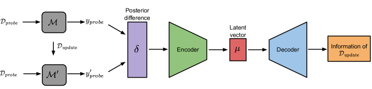
Figure 1: A schematic view of the general attack pipeline.

2.3 Datasets Description

For our experimental evaluation, we use three datasets: MNIST, CIFAR-10, and Insta-NY. Both MNIST and CIFAR-10 are benchmark datasets for various ML security and privacy tasks. MNIST is a 10-class image dataset, it consists of 70,000 28$\times$28 grey-scale images. Each image contains in its center a handwritten digit. Images in MNIST are equally distributed over 10 classes. CIFAR-10 contains 60,000 32$\times$32 color images. Similar to MNIST, CIFAR-10 is also a 10-class balanced dataset. Insta-NY [6] contains a sample of Instagram users’ location check-in data in New York. Each check-in represents a user visiting a certain location at a certain time. Each location is affiliated with a category. In total, there are eight different categories. Our ML task for Insta-NY is to predict each location’s category. We use the number of check-ins happened at each location in each hour on a weekly base as the location’s feature vector. We further filter out locations with less than 50 check-ins, in total, we have 19,215 locations for the dataset. In Section 6, we further use Insta-LA [6] which contains the check-in data from Los Angeles for our threat model relaxation experiments.

3 General Attack Pipeline

Our general attack pipeline contains three phases. In the first phase, the adversary generates her attack input, i.e., posterior difference. In the second phase, our encoder transforms the posterior difference into a latent vector. In the last phase, the decoder decodes the latent vector to produce different information of the updating set with respect to different attacks. Figure 1 provides a schematic view of our attack pipeline.

In this section, we provide a general introduction for each phase of our attack pipeline. In the end, we present our strategy of deriving data to train our attack models.

3.1 Attack Input

Recall that we aim at investigating the information leaked from posterior difference of a model’s two versions when queried with the same set of data samples. To create this posterior difference, the adversary first needs to pick a set of data samples as her probing set, denoted by $\mathcal{D}_{\it probe}$. In this work, the adversary picks a random sample of data samples (from her local dataset) to form $\mathcal{D}_{\it probe}$. Choosing or crafting [33] a specific set of data samples as the probing set may further improve attack efficiency, we leave this as a future work. Next, the adversary queries the target ML model $\mathcal{M}$ with all samples in $\mathcal{D}_{\it probe}$ and concatenates the received outputs to form a vector $y_{\it probe}$. Then, she probes the updated model $\mathcal{M^{\prime}}$ with samples in $\mathcal{D}_{\it probe}$ and creates a vector $y^{\prime}_{\it probe}$ accordingly. In the end, she sets the posterior difference, denoted by $\delta$, to the difference of both outputs:

$$\delta=y_{\it probe}-y^{\prime}_{\it probe}$$

Note that the dimension of $\delta$ is the product of $\mathcal{D}_{\it probe}$’s cardinality and the number of classes of the target dataset. For this paper, both CIFAR-10 and MNIST are 10-class datasets, while Insta-NY is an 8-class dataset. As our probing set always contains 100 data samples, this indicates the dimension of $\delta$ is 1,000 for CIFAR-10 and MNIST, and 800 for Insta-NY.

3.2 Encoder Design

All our attacks share the same encoder structure, we model it with a multilayer perceptron. The number of layers inside the encoder depends on the dimension of $\delta$: Longer $\delta$ requires more layers in the encoder. As our $\delta$ is a 1,000-dimension vector for the MNIST and CIFAR-10 datasets, and 800-dimension vector for the Insta-NY dataset, we use two fully connected layers in the encoder. The first layer transforms $\delta$ to a 128-dimension vector and the second layer further reduces the dimension to 64. The concrete architecture of our encoder is presented in Appendix B.

3.3 Decoder Structure

Our four attacks aim at inferring different information of $\mathcal{D}_{\it update}$, ranging from sample labels to the updating set itself. Thus, we construct different decoders for different attacks with different techniques. The details of these decoders will be presented in the following sections.

3.4 Shadow Model

Our encoder and decoder need to be trained jointly in a supervised manner. This indicates that we need ground truth data for model training. Due to our minimal assumptions, the adversary cannot get the ground truth from the target model. To solve this problem, we rely on shadow models following previous works [40, 13, 38]. A shadow model is designed to mimic the target model. By controlling the training process of the shadow model, the adversary can derive the ground truth data needed to train her attack models.

As presented in Section 2, our adversary knows (1) the architecture of the target model and (2) a dataset coming from the same distribution as the target dataset. To build a shadow model $\mathcal{M}_{\it shadow}$, the adversary first establishes an ML model with the same structure as the target model. Then, she gets a shadow dataset $\mathcal{D}_{\it shadow}$ from her local dataset (the rest is used as $\mathcal{D}_{\it probe}$) and splits it into two parts: Shadow training set $\mathcal{D}_{\it shadow}^{\it train}$ and shadow updating set $\mathcal{D}_{\it shadow}^{\it update}$. $\mathcal{D}_{\it shadow}^{\it train}$ is used to train the shadow model while $\mathcal{D}_{\it shadow}^{\it update}$ is further split to $m$ datasets: $\mathcal{D}_{\it shadow}^{\it update^{1}}\cdots\mathcal{D}_{\it shadow}^{\it update^{m}}$. The number of samples in each of the $m$ datasets depends on the attack. For instance, our single-sample class attacks require each dataset containing a single sample. The adversary then generates $m$ shadow updated models $\mathcal{M^{\prime}}_{\it shadow}^{1}\cdots\mathcal{M^{\prime}}_{\it shadow}^{m}$ by updating the shadow model $\mathcal{M}_{\it shadow}$ with $m$ shadow updating sets in parallel.

The adversary, in the end, probes the shadow and updated shadow models with her probing set $\mathcal{D}_{\it probe}$, and calculates the shadow posterior difference $\delta_{\it shadow}^{1}\cdots\delta_{\it shadow}^{m}$. Together with the corresponding shadow updating set’s ground truth information (depending on the attack), the training data for her attack model is derived.

More generally, the training set for each of our attack models contains $m$ samples corresponding to $\mathcal{D}_{\it shadow}^{\it update^{1}}\cdots\mathcal{D}_{\it shadow}^{\it update^{m}}$. In all our experiments, we set $m$ to 10,000. In addition, we create 1,000 updated models for the target model, this means the testing set for each attack model contains 1,000 samples, corresponding to $\mathcal{D}_{\it target}^{\it update^{1}}\cdots\mathcal{D}_{\it target}^{\it update^{1,000}}$.

4 Single-sample Attacks

In this section, we concentrate on the case when an ML model is updated with a single sample. This is a simplified attack scenario and we aim to examine the possibility of using posterior difference to infer information about the updating set. We start by introducing the single-sample label inference attack, then, present the single-sample reconstruction attack.

4.1 Single-sample Label Inference Attack

Attack Definition. Our single-sample label inference attack takes the posterior difference as the input and outputs the label of the single updating sample. More formally, given a posterior difference $\delta$, our single-sample label inference attack is defined as follows:

$$\mathcal{A}_{\it LI}:\delta\mapsto\ell$$

where $\ell$ is a vector with each entry representing the probability of the updating sample affiliated with a certain label.

Methodology. To recap, the general construction of the attack model consists of an MLP-based encoder which takes the posterior difference as its input and outputs a latent vector $\mu$. For this attack, the adversary constructs her decoder also with an MLP which is assembled with a fully connected layer and a softmax layer to transform the latent vector to the corresponding updating sample’s label. The concrete architecture of our $\mathcal{A}_{\it LI}$’s decoder is presented in Appendix C.

To obtain the data for training $\mathcal{A}_{\it LI}$, the adversary generates ground truth data by creating a shadow model as introduced in Section 3 while setting the shadow updating set’s cardinality to 1. Then, the adversary trains her attack model $\mathcal{A}_{\it LI}$ with a cross-entropy loss. Our loss function is,

$$\mathcal{L}_{\it CE}=\sum\limits_{i}\ell_{i}\log(\hat{\ell}_{i})$$

where $\ell_{i}$ is the true probability of label $i$ and $\hat{\ell}_{i}$ is our predicted probability of label $i$. The optimization is performed by the ADAM optimizer.

To perform the label inference attack, the adversary constructs the posterior difference as introduced in Section 3, then feeds it to the attack model $\mathcal{A}_{\it LI}$ to obtain the label.

Experimental Setup. We evaluate the performance of our single-sample label inference attack using the MNIST, CIFAR-10, and Insta-NY datasets. First, we split each dataset into three disjoint datasets: The target dataset $\mathcal{D}_{\it target}$, the shadow dataset $\mathcal{D}_{\it shadow}$, and the probing dataset $\mathcal{D}_{\it probe}$. As mentioned before, $\mathcal{D}_{\it probe}$ contains 100 data samples. We then split $\mathcal{D}_{\it shadow}$ to $\mathcal{D}_{\it shadow}^{\it train}$ and $\mathcal{D}_{\it shadow}^{\it update}$ to train the shadow model as well as updating it (see Section 3). The same process is applied to train and update the target model with $\mathcal{D}_{\it target}$. As mentioned in Section 3, we build 10,000 and 1,000 updated models for shadow and target models, respectively. This means the training and testing sets for our attack model contain 10,000 and 1,000 samples, respectively.

We use convolutional neural network (CNN) to build shadow and target models for both CIFAR-10 and MNIST datasets, and a multilayer perceptron (MLP) for the Insta-NY dataset. The CIFAR-10 model consists of two convolutional layers, one max pooling layer, three fully connected layers, and a softmax layer. The MNIST model consists of two convolutional layers, two fully connected layers, and a softmax layer. Finally, the Insta-NY model consists of three fully connected layers and a softmax layer. The concrete architectures of the models are presented in Appendix A.

All shadow and target models’ training sets contain 10,000 images for CIFAR-10 and MNIST, and 5,000 samples for Insta-NY. We train the CIFAR-10, MNIST and Insta-NY models for 50, 25, and 25 epochs, respectively, with a batch size of 64. To create an updated ML model, we perform a single-epoch training. Finally, we adopt accuracy to measure the performance of the attack. All of our experiments are implemented using Pytorch [3]. For reproducibility purposes, our code will be made available.

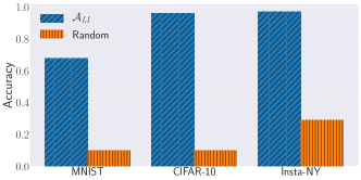
Figure 2: [Higher is better] Performance of the single-sample label inference attack ($\mathcal{A}_{\it LI}$) on MNIST, CIFAR-10, and Insta-NY datasets together with the baseline model. Accuracy is adopted as the evaluation metric.

Results. Figure 2 depicts the experimental results. As we can see, $\mathcal{A}_{\it LI}$ achieves a strong performance with an accuracy of 0.97 on the Insta-NY dataset, 0.96 on the CIFAR-10 dataset, and 0.68 on the MNIST dataset. Moreover, our attack significantly outperforms the baseline model, namely Random, which simply guesses a label over all possible labels. As both CIFAR-10 and MNIST contain 10 balanced classes, the baseline model’s result is approximately 10%. For the Insta-NY dataset, since it is not balanced, we randomly sample a label for each sample to calculate the baseline which results in approximately 29% accuracy. Our evaluation shows that the different outputs of an ML model’s two versions indeed leak information of the corresponding updating set.

4.2 Single-sample Reconstruction Attack

Figure 3: Methodology of the single-sample reconstruction attack ($\mathcal{A}_{\it SSR}$).

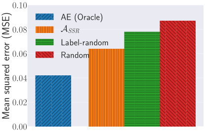
(a) MNIST

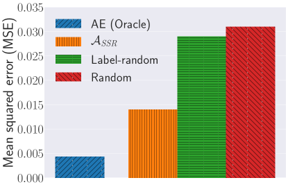
(b) CIFAR-10

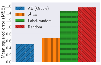
(c) Insta-NY

Figure 4: [Lower is better] Performance of the single-sample reconstruction attack ($\mathcal{A}_{\it SSR}$) together with autoencoder and two baseline models. Mean squared error is adopted as the evaluation metric. Autoencoder (AE) serves as an oracle as the adversary cannot use it for her attack.

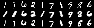
Figure 5: Visualization of some generated samples from the single-sample reconstruction attack ($\mathcal{A}_{\it SSR}$) on the MNIST dataset. Samples are fair random draws, not cherry-picked. The first row shows the original samples. The second row shows the reconstructed samples by $\mathcal{A}_{\it SSR}$. The third shows row the reconstructed samples by autoencoder, i.e., the upper bound of our reconstruction attack.

Attack Definition. Our single-sample reconstruction attack takes one step further to construct the data sample used to update the model. Formally, given a posterior difference $\delta$, our single-sample reconstruction attack, denoted by $\mathcal{A}_{\it SSR}$, is defined as follows:

$$\mathcal{A}_{\it SSR}:\delta\mapsto x_{\it update}$$

where $x_{\it update}$ denotes the sample used to update the model ($\mathcal{D}_{\it update}=\{x_{\it update}\}$).

Methodology. Reconstructing a data sample is a much more complex task than predicting the sample’s label. To tackle this problem, we need an ML model which is able to generate a data sample in the complex space. To this end, we rely on autoencoder (AE).

Autoencoder is assembled with an encoder and a decoder. Different from our attacks, AE’s goal is to learn an efficient encoding for a data sample: Its encoder encodes a sample into a latent vector and its decoder tries to decode the latent vector to reconstruct the same sample. This indicates AE’s decoder itself is a data sample reconstructor. For our attack, we first train an AE, then transfer the AE’s decoder to our attack model as the initialization of the attack’s decoder. Figure 3 provides an overview of the attack methodology. The concrete architectures of our AEs’ encoders and decoders are presented in Appendix D.

After the autoencoder is trained, the adversary takes its decoder and appends it to her attack model’s encoder. To establish the link, the adversary adds an additional fully connected layer to its encoder which transforms the dimensions of the latent vector $\mu$ to the same dimension as $\mu_{\it AE}$.

We divide the attack model training process into two phases. In the first phase, the adversary uses her shadow dataset to train an AE with the previously mentioned model architecture. In the second phase, she follows the same procedure for single-sample label inference attack to train her attack model. Note that the decoder from AE here serves as the initialization of the decoder, this means it will be further trained together with the attack model’s encoder. To train both autoencoder and our attack model, we use mean squared error (MSE) as the loss function. Our objective is,

$$\mathcal{L}_{\it MSE}=\lVert\hat{x}_{\it update}-x_{\it update}\lVert^{2}_{2}$$

where $\hat{x}_{\it update}$ is our predicted data sample. We again adopt ADAM as the optimizer.

Experimental Setup. We use the same experimental setup as the previous attack (see Section 4.1) except for the evaluation metric. In detail, we adopt MSE to measure our attack’s performance instead of accuracy.

We construct two baseline models, namely Label-random and Random. Both of these baseline models take a random data sample from the adversary’s shadow dataset. The difference is that the Label-random baseline picks a sample within the same class as the target updating sample, while the Random baseline takes a random data sample from the whole shadow dataset of the adversary. The Label-random baseline can be implemented by first performing our single-sample label inference attack to learn the label of the data sample and then picking a random sample affiliated with the same label.

Results. First, our single-sample reconstruction attack achieves a promising performance. As shown in Figure 4, our attack on the MNIST dataset outperforms the Random baseline by 36% and more importantly, outperforms the Label-random baseline by 22%. Similarly, for the CIFAR-10 and Insta-NY datasets, our attack achieves an MSE of 0.014 and 0.68 which is significantly better than the two baseline models, i.e., it outperforms the Label-random (Random) baselines by a factor of 2.1 (2.2) and 2.1 (2.3), respectively. The difference between our attack’s performance gain over the baseline models on the MNIST and on the other datasets is expected as the MNIST dataset is more homogeneous compared to the other two. In other words, the chance of picking a random data sample similar to the updating sample is much higher in the MNIST dataset than in the other datasets.

Secondly, we compare our attack’s performance against the results of the autoencoder for sample reconstruction. Note that AE takes the original data sample as input and outputs the reconstructed one, thus it is considered as an oracle, since the adversary does not have access to the original updating sample. Here, we just use AE’s result to show the best possible result for our attack. From Figure 4, we observe that AE achieves 0.042, 0.0043, and 0.51 MSE for the MNIST, CIFAR-10, and Insta-NY datasets, respectively, which indeed outperforms our attack. However, our attack still has a comparable performance.

Finally, Figure 5 visualizes some randomly sampled reconstructed images by our attack on MNIST. The first row depicts the original images used to update the models and the second row shows the result of our attack. As we can see, our attack is able to reconstruct images that are visually similar to the original sample with respect to rotation and shape. We also show the result of AE in the third row in Figure 5 which as mentioned before, is the upper bound for our attack. The results from Figure 4 and Figure 5 demonstrate the strong performance of our attack.

5 Multi-sample Attacks

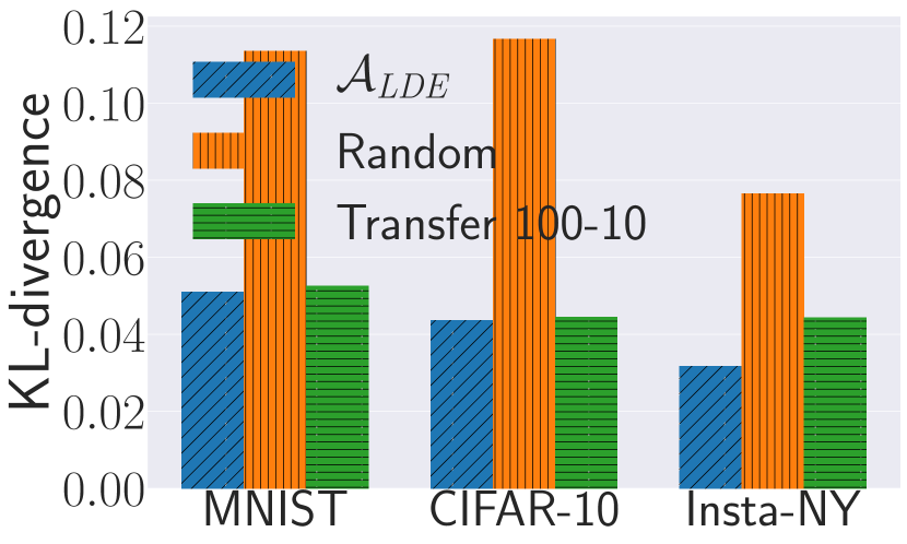
(a) KL-divergence (10 samples)

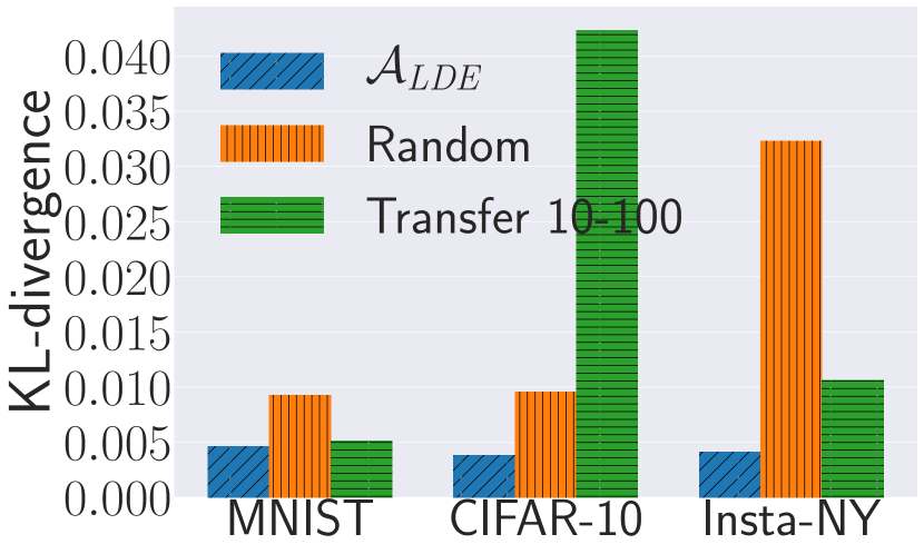
(b) KL-divergence (100 samples)

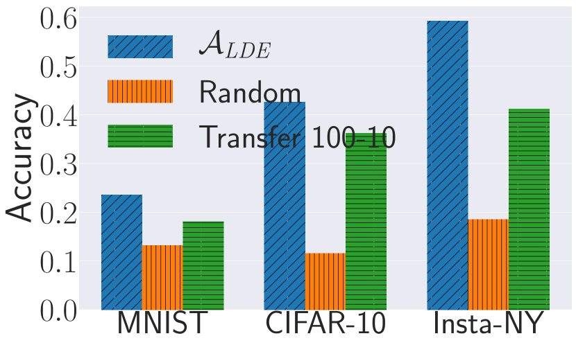
(c) Accuracy (10 samples)

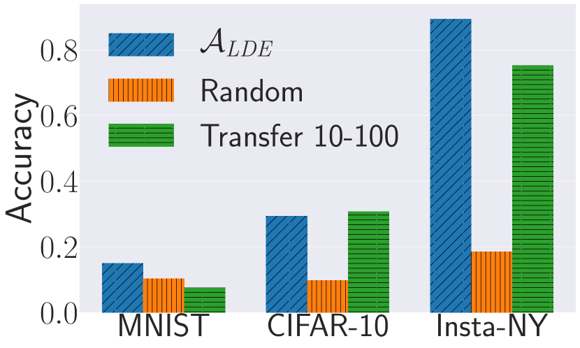
(d) Accuracy (100 samples)

Figure 6: [Lower is better for (a) and (b), higher is better for (c) and (d)] Performance of the multi-sample label distribution estimation attack ($\mathcal{A}_{\it LDE}$) together with the baseline model and transfer attack. KL-divergence and accuracy are adopted as the evaluation metric. Accuracy here is used to measure the prediction of the most frequent label over samples in the updating set. Transfer 10-100 means each of the training sample for the attack model corresponds to an updating set containing 10 data samples and each of the testing sample for the attack model corresponds to an updating set containing 100 data samples.

After demonstrating the effectiveness of our attacks against the updating set with a single sample, we now focus on a more general attack scenario where the updating set contains multiple data samples that are never seen during the training. We introduce two attacks in the multi-sample attack class: Multi-sample label distribution estimation attack and multi-sample reconstruction attack.

5.1 Multi-sample Label Distribution Estimation Attack

Attack Definition. Our first attack in the multi-label attack class aims at estimating the label distribution of the updating set’s samples. It can be considered as a generalization of the label inference attack in the single-sample attack class. Formally, the attack is defined as:

$$\mathcal{A}_{\it LDE}:\delta\mapsto q$$

where $q$ as a vector denotes the distribution of labels over all classes for samples in the updating set.

Methodology. The adversary uses the same encoder structure as presented in Section 3 and the same decoder structure of the label inference attack (Section 4.1). Since the label distribution estimation attack estimates a probability vector $q$ instead of performing classification, we use Kullback-–Leibler divergence (KL-divergence) as our objective function:

$$\mathcal{L}_{\it KL}=\sum\limits_{i}(\hat{q}_{\ell})_{i}\log\frac{(\hat{q}_{\ell})_{i}}{(q_{\ell})_{i}}$$

where $\hat{q}_{\ell}$ and $q_{\ell}$ represent our attack’s estimated label distribution and the target label distribution, respectively, and $(q_{\ell})_{i}$ corresponds to the $i$th label.

To train the attack model $\mathcal{A}_{\it LDE}$, the adversary first generates her training data as mentioned in Section 3. She then trains $\mathcal{A}_{\it LDE}$ with the posterior difference $\delta_{\it shadow}^{1}\cdots\delta_{\it shadow}^{m}$ as the input and the normalized label distribution of their corresponding updating sets as the output. We assume the adversary knows the cardinality of the updating set. We try to relax this assumption later in our evaluation.

Experimental Setup. We evaluate our label distribution estimation attack using updating set of cardinalities 10 and 100. For the two different cardinalities, we build attack models as mentioned in the methodology. All data samples in each updating set for the shadow and target models are sampled uniformly, thus each sample (in both training and testing set) for the attack model, which corresponds to an updating set, has the same label distribution of the original dataset. We use a batch size of 64 when updating the models.

For evaluation metrics, we calculate KL-divergence for each testing sample (corresponding to an updating set on the target model) and report the average result over all testing samples (1,000 in total). Besides, we also measure the accuracy of predicting the most frequent label over samples in the updating set. We randomly sample a dataset with the same size as the updating set and use its samples’ label distribution as the baseline, namely Random.

Results. We report the result for our label distribution estimation attack in Figure 6. As shown, $\mathcal{A}_{\it LDE}$ achieves a significantly better performance than the Random baseline on all datasets. For the updating set with 100 data samples on the CIFAR-10 dataset, our attack achieves 3 and 2.5 times better accuracy and KL-divergence, respectively, than the Random baseline. Similarly, for the MNIST and Insta-NY datasets, our attack achieves 1.5 and 4.8 times better accuracy, and 2 and 7.9 times better KL-divergence. Furthermore, $\mathcal{A}_{\it LDE}$ achieves a similar improvement over the Random baseline for the updating set of size 10.

Recall that the adversary is assumed to know the cardinality of the updating set in order to train her attack model, we further test whether we can relax this assumption. To this end, we first update the shadow model with 100 samples while updating the target model with 10 samples. As shown in 6(a) and 6(c) Transfer 100-10, our attack still has a similar performance as the original attack. However, when the adversary updates her shadow model with 10 data samples while the target model is updated with 100 data samples (6(b) and 6(d) Transfer 10-100), our attack performance drops significantly, in particular for KL-divergence on the CIFAR-10 dataset. We believe this is due to the 10 samples not providing enough information for the attack model to generalize to a larger updating set.

5.2 Multi-sample Reconstruction Attack

Attack Definition. Our last attack, namely multi-sample reconstruction attack, aims at reconstructing the updating set. This attack can be considered as a generalization of the single-sample reconstruction attack, and a step towards the goal of reconstructing the training set of a black-box ML model. Formally, the attack is defined as follows:

$$\mathcal{A}_{\it MSR}:\delta\mapsto\mathcal{D}_{\it update}$$

where $\mathcal{D}_{\it update}=\{x^{1}_{\it update},\dots,x^{|\mathcal{D}_{\it update}|}_{\it update}\}$ contains the samples used to update the model.

Methodology. The complexity of the task for reconstructing an updating set increases significantly when the updating set size grows from one to multiple. Our single-sample reconstruction attack (Section 4.2) uses AE to reconstruct a single sample. However, AE cannot generate a set of samples. In fact, directly predicting a set of examples is a very challenging task. Therefore, we rely on generative models which are able to generate multiple samples rather than a single one.

We first introduce the classical Generative Adversarial Networks (GANs) and point out why classical GANs cannot be used for our multi-sample reconstruction attack. Next, we propose our Conditional Best of Many GAN (CBM-GAN), a novel hybrid generative model and demonstrate how to use it to execute the multi-sample reconstruction attack.

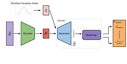
Figure 7: Methodology of the multi-sample reconstruction attack ($\mathcal{A}_{\it MSR}$).

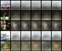
(a)

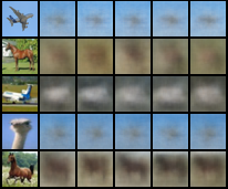
(b)

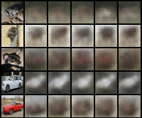
(c)

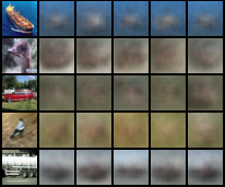
(d)

Figure 8: Visualization of some generated samples from the multi-sample reconstruction attack ($\mathcal{A}_{\it MSR}$) before clustering on the CIFAR-10 dataset. Samples are fair random draws, not cherry-picked. The left column shows the original samples and the next 5 columns show the 5 nearest reconstructed samples with respect to mean squared error.

Generative Adversarial Networks. Samples from a dataset are essentially samples drawn from a complex data distribution. Thus, one way to reconstruct the dataset $\mathcal{D}_{\it update}$ is to learn this complex data distribution and sample from it. This is the approach we adopt for our multi-sample reconstruction attack. Mainly, the adversary starts the attack by learning the data distribution of $\mathcal{D}_{\it update}$, then she generates multiple samples from the learned distribution, which is equivalent to reconstructing the dataset $\mathcal{D}_{\it update}$. In this work, we leverage the state-of-the-art generative model GANs, which has been demonstrated effective on learning a complex data distribution.

A GAN consists of a pair of ML models: a generator (G) and a discriminator (D). The generator G learns to transform a Gaussian noise vector $z\sim\mathcal{N}(0,1)$ to a data sample $\hat{x}$,

$$\text{G}:z\mapsto\hat{x}$$

such that the generated sample $\hat{x}$ is indistinguishable from a true data sample. This is enabled by the discriminator D which is jointly trained. The generator G tries to fool the discriminator, which is trained to distinguish between samples from the Generator (G) and true data samples. The objective function maximized by GAN’s discriminator D is,

$$\mathcal{L}_{D}=\mathbb{E}_{x\in\mathcal{D}_{\it update}}\log(\text{D}(x))+\mathbb{E}_{\hat{x}}\log(1-\text{D}(\hat{x}))$$ (1)

The GAN discriminator D is trained to output 1 (“true”) for real data and 0 (“false”) for fake data. On the other hand, the generator G maximizes:

$$\mathcal{L}_{G}=\mathbb{E}_{\hat{x}}\log(\text{D}(\hat{x}))$$

Thus, G is trained to produce samples $\hat{x}=\text{G}(z)$ that are classified as “true” (real) by D.

However, our attack aims to reconstruct $\mathcal{D}_{\it update}$ for any given $\delta$, which the standard GAN does not support. Therefore, first, we change the GAN into a conditional model to condition its generated samples $\hat{x}$ on the posterior difference $\delta$. Second, we construct our novel hybrid generative model CBM-GAN, by adding a new “Best Match” loss to reconstruct all samples inside the updating set accurately.

CBM-GAN. The decoder of our attack model is casted as our CBM-GAN’s generator (G). To enable this, we concatenate the noise vector $z$ and the latent vector $\mu$ produced by our attack model’s encoder (with posterior different as input), and use it as CBM-GAN’s generator’s input, as in Conditional GANs [30]. This allows our decoder to map the posterior difference $\delta$ to samples in $\mathcal{D}_{\it update}$.

However, Conditional GANs are severely prone to mode collapse, where the generator’s output is restricted to a limited subset of the distribution [7, 51]. To deal with this, we introduce a reconstruction loss. This reconstruction loss forces our GAN to cover all the modes of the distribution (set) of data samples used to update the model. However, it is unclear, given a posterior difference $\delta$ and a noise vector $z$ pair, which sample in the data distribution we should force CBM-GAN to reconstruct. Therefore, we allow our GAN full flexibility in learning a mapping from posterior difference and noise vector $z$ pairs to data samples – this means we allow it to choose the data sample to reconstruct. We realize this using a novel “Best Match” based objective in the CBM-GAN formulation,

$$\mathcal{L}_{BM}=\sum_{x\in\mathcal{D}_{\it update}}\min\limits_{\hat{x}\sim\text{G}}\lVert\hat{x}-x\lVert^{2}_{2}\,+\sum_{\hat{x}}\,\log(\text{D}(\hat{x}))$$ (2)

where $\hat{x}\sim\text{G}$ represents samples produced by our CBM-GAN given a latent vector $\mu$ and noise sample $z$. The first part of the $\mathcal{L}_{BM}$ objective is based on the standard MSE reconstruction loss and forces our CBM-GAN to reconstruct all samples in $\mathcal{D}_{\it update}$ as the error is summed across $x\in\mathcal{D}_{\it update}$. However, unlike the standard MSE loss, given a data sample $x\in\mathcal{D}_{\it update}$, the loss is based only on the generated sample $\hat{x}$ which is closest to the data sample $x\in\mathcal{D}_{\it update}$. This allows CBM-GAN to reconstruct samples in $\mathcal{D}_{\it update}$ without having an explicit mapping from posterior difference and noise vector $z$ pairs to data samples, as only the “Best Match” is penalized. Finally, the discriminator D ensures that the samples $\hat{x}$ are indistinguishable from the “true” samples of $\mathcal{D}_{\it update}$.

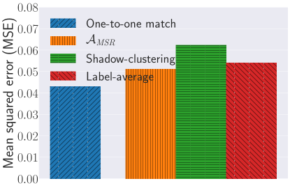
(a) MNIST

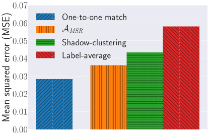
(b) CIFAR-10

(c) Insta-NY

Figure 9: [Lower is better] Performance of the multi-sample reconstruction attack ($\mathcal{A}_{\it MSR}$) together with one-to-one match and the two baseline models. Mean squared error (MSE) is adopted as the evaluation metric. The match between the original and reconstructed samples is performed by the Hungarian algorithm for both $\mathcal{A}_{\it MSR}$ and Shadow-clustering. For Label-average, each sample is matched within the average of samples with the same class in the shadow dataset. One-to-one match serves as an oracle as the adversary cannot use it for her attack.

Training of CBM-GAN. The training of the attack model $\mathcal{A}_{\it MSR}$ is more complicated than previous attacks, hence we provide more details here. Similar to the previous attacks, the adversary starts the training by generating the training data as mentioned in Section 3. She then jointly trains her encoder and CBM-GAN with the posterior difference $\delta_{\it shadow}^{1}\cdots\delta_{\it shadow}^{m}$ as the inputs and samples inside their corresponding updating sets, i.e., $\mathcal{D}_{\it shadow}^{\it update^{1}}\cdots\mathcal{D}_{\it shadow}^{\it update^{m}}$ as the output. More concretely, for each posterior difference $\delta_{\it shadow}^{i}$, she updates her attack model $\mathcal{A}_{\it MSR}$ as follows:

1. The adversary sends the posterior difference $\delta_{\it shadow}^{i}$ to her encoder to get the latent vector $\mu_{i}$.

2. She then generates $|\mathcal{D}_{\it shadow}^{\it update^{i}}|$ noise vectors.

3. To create generator’s input, she concatenates each of the noise vectors with the latent vector $\mu_{i}$.

4. On the input of the concatenated vectors, the CBM-GAN generates $|\mathcal{D}_{\it shadow}^{\it update^{i}}|$ samples, i.e., each vector corresponds to each sample.

5. The adversary then calculates the generator loss as introduced by Equation 2, and uses it to update the generator and the encoder.

6. Finally, she calculates and updates the CBM-GAN’s discriminator according to Equation 1.

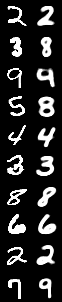
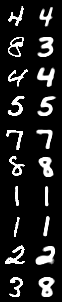
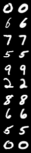
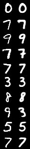
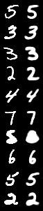
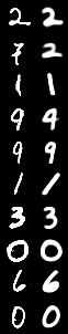
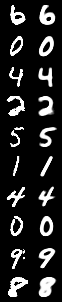
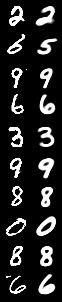
Figure 10: Visualization of a full MNIST updating set together with the output of the multi-sample reconstruction attack ($\mathcal{A}_{\it MSR}$) after clustering. Samples are fair random draws, not cherry-picked. The left column shows the original samples and the right column shows the reconstructed samples. The match between the original and reconstructed samples is performed by the Hungarian algorithm.

Clustering. CBM-GAN only provides a generator which learns the distribution of the samples in the updating set. However, to reconstruct the exact data samples in $\mathcal{D}_{\it update}$, we need a final step assisted by machine learning clustering. In detail, we assume the adversary knows the cardinality of $\mathcal{D}_{\it update}$ as in Section 5.1. After CBM-GAN is trained, the adversary utilizes CBM-GAN’s generator to generate a large number of samples. She then clusters the generated samples into $|\mathcal{D}_{\it update}|$ clusters. Here, the K-means algorithm is adopted to perform clustering where we set K to $|\mathcal{D}_{\it update}|$. In the end, for each cluster, the adversary calculates its centroid, and takes the nearest sample to the centroid as one reconstructed sample.

Figure 7 presents a schematic view of our multi-sample reconstruction attack’s methodology. The concrete architecture of CBM-GAN’s generator and discriminator for the three datasets used in this paper are listed in Appendix E.

Experimental Setup. We evaluate the multi-sample reconstruction attack on the updating set of size 100 and generate 20,000 samples for each updating set reconstruction with CBM-GAN. For the rest of the experimental settings, we follow the one mentioned in Section 5.1 except for evaluation metrics and baseline.

We use MSE between the updating and reconstructed data samples to measure the multi-sample reconstruction attack’s performance. We construct two baselines, namely Shadow-clustering and Label-average. For Shadow-clustering, we perform K-means clustering on the adversary’s shadow dataset. More concretely, we cluster the adversary’s shadow dataset into 100 clusters and take the nearest sample to the centroid of each cluster as one reconstructed sample. For Label-average, we calculate the MSE between each sample in the updating set and the average of the images with the same label in the adversary’s shadow dataset.

Results. In Figure 8, we first present some visualization of the intermediate result of our attack, i.e., the CBM-GAN’s output before clustering, on the CIFAR-10 dataset. For each randomly sampled image in the updating set, we show the 5 nearest reconstructed images with respect to MSE generated by CBM-GAN. As we can see, our attack model tries to generate images with similar characteristics to the original images. For instance, the 5 reconstructed images for the airplane image in 8(b) all show a blue background and a blurry version of the airplane itself. The similar result can be observed from the boat image in 8(a), the car image in 8(c), and the boat image in 8(d). It is also interesting to see that CBM-GAN provides different samples for the two different horse images in 8(b). The blurriness in the results is expected, due to the complex nature of the CIFAR-10 dataset and the weak assumptions for our adversary, i.e., access to black-box ML model.

We also quantitatively measure the performance of our intermediate results, by calculating the MSE between each image in the updating set and its nearest reconstructed sample. We refer to this as one-to-one match. Figure 9 shows for the CIFAR-10, MNIST, and Insta-NY datasets, we achieve 0.0283, 0.043 and 0.60 MSE, respectively. It is important to note that the adversary cannot perform one-to-one match as she does not have access to ground truth samples in the updating set, i.e., one-to-one match is an oracle.

Figure 9 shows the mean squared error of our full attack with clustering for all datasets. To match each of our reconstructed samples to a sample in $\mathcal{D}_{\it update}$, we rely on the Hungarian algorithm [24]. This guarantees that each reconstructed sample is only matched with one ground truth sample in $\mathcal{D}_{\it update}$ and vice versa. As we can see, our attack outperforms both baseline models on the CIFAR-10, MNIST and Insta-NY datasets (20%, 22%, and 25% performance gain for Shadow-clustering and 60.1%, 5.5% and 14% performance gain for Label-average, respectively). The different performance gain of our attack over the label-average baseline for different datasets is due to the different complexity of these datasets. For instance, all images inside MNIST have black background and lower variance within each class compared to the CIFAR-10 dataset. The different complexity results in some datasets having a more representative label-average, which leads to a lower performance gain of our attack over them.

These results show that our multi-sample reconstruction attack provides a more useful output than calculating the average from the adversary’s dataset. In detail, our attack achieves an MSE of 0.036 on the CIFAR-10 dataset, 0.051 on the MNIST dataset, and 0.64 on the Insta-NY dataset. As expected, the MSE of our final attack is higher than one-to-one match, i.e., the above mentioned intermediate results.

We further visualize our full attack’s result on the MNIST dataset. Figure 10 shows a sample of a full MNIST updating set reconstruction, i.e., the CBM-GAN’s reconstructed images for the 100 original images in an updating set. We observe that our attack model reconstructs diverse digits of each class that for most of the cases match the actual ground truth data very well. This suggests CBM-GAN is able to capture most modes in a data distribution well. Moreover, comparing the results of this attack (Figure 10) with the results of the single-sample reconstruction attack (Figure 5), we can see that this attack produces sharper images. This result is due to the discriminator of our CBM-GAN, as it is responsible for making the CBM-GAN’s output to look real, i.e., sharper in this case.

One limitation of our attack is that CBM-GAN’s sample generation and clustering are performed separately. In the future, we plan to combine them to perform an end-to-end training which may further boost our attack’s performance.

From all these results, we show that our attack does not generate a general representation of data samples affiliated with the same label, but tries to reconstruct images with similar characteristics as the images inside the updating set (as shown by the different shapes of the same numbers in Figure 10).

Relaxing The Knowledge of Updating Set Cardinality. One of the above attack’s main assumptions is the adversary’s knowledge of the updating set cardinality, i.e., $|\mathcal{D}_{\it update}|$. Next, we show how to relax this assumption. To recap, the adversary needs the updating set cardinality when updating her shadow model and clustering CBM-GAN’s output. We address the former by using updating sets of different cardinalities. For the latter, we use the silhouette score to find the optimal k for K-means, i.e., the most likely value of the target updating set’s cardinality. The silhouette score lies in the range between -1 and 1, it reflects the consistency of the clustering. Higher silhouette score leads to more suitable k.

Specifically, the adversary follows the previously presented methodology in Section 5.2 with the following modifications. First, instead of using updating sets with the same cardinality, the adversary uses updating sets with different cardinalities to update the shadow model. Second, after the adversary generates multiple samples from CBM-GAN, she uses the silhouette score to find the optimal k. The silhouette score is used here to identify the target model’s updating set cardinality from the different updating sets cardinalities used to update the shadow model.

We evaluate the effectiveness of this attack on all datasets. We use a target model updated with 100 samples and create our shadow updated models using updating sets with cardinality 10 and 100. Concretely, we update the shadow model half of the time with updating sets of cardinality 10 and the other half with cardinality 100.

Our evaluation shows that our attack consistently produces higher silhouette score -by at least 20%- for the correct cardinality in all cases. In another way, our method can always detect the right cardinality of the updating set in this setting. Moreover, the MSE for the final output of the attack only drops by 1.6%, 0.8%, and 5.6% for the Insta-NY, MNIST, and CIFAR-10 datasets, respectively.

6 Discussion

In this section, we analyze the effect of different hyperparameters of both the target and shadow models on our attacks’ performance. Furthermore, we investigate relaxing the threat model assumptions and discuss the limitations of our attacks.

Relaxing The Attacker Model Assumption. Our threat model has two main assumptions: Same data distribution for both target and shadow datasets and same structure for both target and shadow models. We relax the former by proposing data transferability attack and latter by model transferability attack.

Attack	Original	Transfer
$\mathcal{A}_{\it LI}$	0.97	0.89
$\mathcal{A}_{\it SSR}$	0.68	1.1
$\mathcal{A}_{\it LDE}(10)$	0.59(0.0317)	0.55(0.0377)
$\mathcal{A}_{\it LDE}(100)$	0.89(0.0041)	0.89 (0.0067)
$\mathcal{A}_{\it MSR}$	0.64	0.73

Table 1: Evaluation of the data transferability attacks. The first column shows all different attacks, the second and third shows the performance of the attacks using similar and different distributions, respectively. Where $\mathcal{A}_{\it LI}$ performance is measured in accuracy, $\mathcal{A}_{\it MSR}$ and $\mathcal{A}_{\it SSR}$ measured in MSE, and $\mathcal{A}_{\it LDE}(10)$ and $\mathcal{A}_{\it LDE}(100)$ measured in accuracy (KL-divergence).

Data Transferability. In this setting, we locally train and update the shadow model with a dataset which comes from a different distribution from the target dataset. For our experiments, we use Insta-NY as the target dataset and Insta-LA as the shadow dataset.

Table 1 depicts the evaluation results. As expected, the performance of our data transferability attacks drops; however, they are still significantly better than corresponding baseline models. For instance, the performance of the multi-sample reconstruction attack drops by 14% but is still 10% better than the baseline (see Figure 9). Moreover, the multi-sample label distribution attack’s accuracy (KL-divergence) only drops by 6.8% (18.9%) and 0% (63%), which is still significantly better than the baseline (see Figure 6) by 6.5x (2x) and 4.6x (4.8x) for updating set sizes of 10 and 100, respectively.

Model Transferablity. Now we relax the attacker’s knowledge on the target model’s architecture, i.e., we use different architectures for shadow and target models. In our experiments on Insta-NY, we use the same architecture mentioned previously in Section 4.1 for the target model, and remove one hidden layer and use half of the number of neurons in other hidden layers for the shadow model.

The performance drop of our model transferability attack is only less than 2% for all of our attacks, which shows that our attacks are robust against such changes in the model architectures. We observe similar results when repeating the experiment using different architectures and omit them for space restrictions.

Effect of The Probing Set Cardinality. We evaluate the performance of our attacks on CIFAR-10 when the probing set cardinality is 10, 100, 1,000, or 10,000. As our encoder’s input size relies on the probing set cardinality (see Section 3), we adjust its input layer size accordingly.

As expected, using a probing set of size 10 reduces the performance of the attacks. For instance, the single-sample label inference and reconstruction attacks’ performance drops by 9% and 71%, respectively. However, increasing the probing set cardinality from 100 to 1,000 or 10,000 has a limited effect (up to 3.5% performance gain). It is also important to mention that the computational requirement for our attacks increases with an increasing probing set cardinality, as the cardinality decides the size of the input layer for our attack models. In conclusion, using 100 samples for probing the target model is a suitable choice.

Effect of Target Model Hyperparameters. We now evaluate our attacks’ performance with respect to two hyperparameters of the target model.

Target Model’s Training Epochs Before Updating. We use the MNIST dataset to evaluate the multi-sample label distribution estimation attack’s performance on target models trained for 10, 20, and 50 epochs. For each setting, we update the model and execute our attack as mentioned in Section 5.1.

The experiments show that the difference in the attack’s performance for the different models is less than 2%. That is expected as gradients are not monotonically decreasing during the training procedure. In other words, information is not necessarily vanishing [15].

Target Model’s Updating Epochs. We train target and shadow models as introduced in Section 5.1 with the Insta-NY dataset, but we update the models using different number of epochs. More concretely, we update the models using from 2 to 10 epochs and evaluate the multi-sample label distribution estimation attack’s performance on the updated models.

We report the results of our experiments in Figure 11. As expected, the multi-sample label distribution estimation attack’s performance improves with the increase of the number of epochs used to update the model. For instance, the attack performance improves by 25.4 % when increasing the number of epochs used to update the model from 2 to 10.

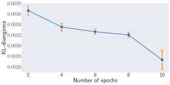
Figure 11: [Lower is better] The performance of the multi-sample label distribution estimation attack ($\mathcal{A}_{\it LDE}$) with different number of epochs used to update the target model.

Limitations of Our Attacks. For all of our attacks, we assume a simplified setting, in which, the target model is solely updated on new data. Moreover, we perform our attacks on updating sets of maximum cardinality of 100. In future work, we plan to further investigate a more complex setting, where the target model is updated using larger updating sets of both new and old data.

7 Possible Defenses

Adding Noise to Posteriors. All our attacks leverage posterior difference as the input. Therefore, to reduce our attacks’ performance, one could sanitize posterior difference. However, the model owner cannot directly manipulate the posterior difference, as she does not know with what or when the adversary probes her model. Therefore, she has to add noise to the posterior for each queried sample independently. We have tried adding noise sampled from a uniform distribution to the posteriors. Experimental results show that the performance for some of our attacks indeed drops to a certain degree. For instance, the single-sample label inference attack on the CIFAR-10 dataset drops by 17% in accuracy. However, the performance of our multi-sample reconstruction attack stays stable. One reason might be the noise vector $z$ is part of CBM-GAN’s input which makes the attack model more robust to the noisy input.

Differential Privacy. Another possible defense mechanism against our attacks is differentially private learning. Differential privacy [10] can help an ML model learn its main tasks while reducing its memory on the training data. If differentially private learning schemes [4, 39, 9] are used when updating the target ML model, this by design will reduce the performance of our attacks. However, it is also important to mention that depending on the privacy budget for differential privacy, the utility of the model can drop significantly.

We leave an in-depth exploration of effective defense mechanisms against our attacks as a future work.

8 Related Works

Membership Inference. Membership inference aims at determining whether a data sample is inside a dataset. It has been successfully performed in various settings, such as biomedical data [21, 18] and location data [36, 37]. Shokri et al. [40] propose the first membership inference attack against machine learning models. In this attack, an adversary’s goal is to determine whether a data sample is in the training set of a black-box ML model. To mount this attack, the adversary relies on a binary machine learning classifier which is trained with the data derived from shadow models (similar to our attacks). More recently, multiple membership inference attacks have been proposed with new attacking techniques or targeting on different types of ML models [27, 19, 28, 53, 31, 42, 38, 32].

In theory, membership inference attack can be used to reconstruct the dataset, similar to our reconstruction attacks. However, it is not scalable in the real-world setting as the adversary needs to obtain a large-scale dataset which includes all samples in the target model’s training set. Though our two reconstruction attacks are designed specifically for the online learning setting, we believe the underlying techniques we propose, i.e., pretrained decoder from a standard autoencoder and CBM-GAN, can be further extended to reconstruct datasets from black-box ML models in other settings.

Model Inversion. Fredrikson et al. [12] propose model inversion attack first on biomedical data. The goal of model inversion is to infer some missing attributes of an input feature vector based on the interaction with a trained ML model. Later, other works generalize the model inversion attack to other settings, e.g.,, reconstructing recognizable human faces [11, 20]. As pointed out by other works [40, 29], model inversion attack reconstructs a general representation of data samples affiliated with certain labels, while our reconstruction attacks target on specific data samples used in the updating set.

Model Stealing. Another related line of work is model stealing. Tramèr et al. [45] are among the first to introduce the model stealing attack against black-box ML models. In this attack, an adversary tries to learn the target ML model’s parameters. Tramèr et al. propose various attacking techniques including equation-solving and decision tree path-finding. The former has been demonstrated to be effective on simple ML models, such as logistic regression, while the latter is designed specifically for decision trees, a class of machine learning classifiers. Moreover, relying on an active learning based retraining strategy, the authors show that it is possible to steal an ML model even if the model only provides the label instead of posteriors as the output. More recently, Orekondy et al. [34] propose a more advanced attack on stealing the target model’s functionality and show that their attack is able to replicate a mature commercial machine learning API. In addition to model parameters, several works concentrate on stealing ML models’ hyperparameters [33, 47].

Besides the above, there exist a wide range of other attacks and defenses on machine learning models [9, 43, 46, 16, 25, 4, 35, 14, 41, 8, 44, 52, 49, 22, 17, 55, 5, 13, 48, 54, 50, 23, 26, 56]

9 Conclusion

Large-scale data being generated at every second turns ML model training into a continuous process. In consequence, a machine learning model queried with the same set of data samples at two different time points will provide different results. In this paper, we investigate whether these different model outputs can constitute a new attack surface for an adversary to infer information of the dataset used to perform model update. We propose four different attacks in this surface all of which follow a general encoder-decoder structure. The encoder encodes the difference in the target model’s output before and after being updated, and the decoder generates different types of information regarding the updating set.

We start by exploring a simplified case when an ML model is only updated with one single data sample. We propose two different attacks for this setting. The first attack shows that the label of the single updating sample can be effectively inferred. The second attack utilizes an autoencoder’s decoder as the attack model’s pretrained decoder for single-sample reconstruction.

We then generalize our attacks to the case when the updating set contains multiple samples. Our multi-sample label distribution estimation attack trained following a KL-divergence loss is able to infer the label distribution of the updating set’s data samples effectively. For the multi-sample reconstruction attack, we propose a novel hybrid generative model, namely CBM-GAN, which uses a “Best Match’ loss in its objective function. The “Best Match” loss directs CBM-GAN’s generator to reconstruct each sample in the updating set. Quantitative and qualitative results show that our attacks achieve promising performance.

Appendices

Appendix A Target Models Architecture

Here, max($2$) denotes a max-pooling layer with a $2\times 2$ kernel, FullyConnected($x$) denotes a fully connected layer with $x$ hidden units, Conv2d(k’,s’) denotes a 2-dimension convolution layer with kernel size $k^{\prime}\times k^{\prime}$ and $s^{\prime}$ filters, and Softmax denotes the Softmax function. We adopt ReLU as the activation function for all layers for the MNIST, CIFAR-10 and Location models.

Appendix B Encoder Architecture

Here, $\mu$ denotes the latent vector which serves as the input for our decoder. Furthermore, we use LeakyReLU as our encoder’s activation function and apply dropout on both layers for regularization.

Appendix C Single-sample Label Inference Attack’s Decoder Architecture

Here, $n$ is equal to the size of $\ell$, i.e., $n=|\ell|$.

Appendix D Single-sample Reconstruction Attack

D.1 AE’s Encoder Architecture

Here, $\mu_{\it AE}$ is the latent vector output of the encoder. Moreover, $k_{i}$, $s_{i}$, and $f_{i}$ represent the kernel size, number of filters, and number of units in the $i$th layer. The concrete values of these hyperparameters depend on the target dataset, we present our used values in Table 2. We adopt ReLU as the activation function for all layers for the MNIST and CIFAR-10 encoders. For the Insta-NY decoder, we use ELU as the activation function for all layers except for the last one. Finally, we apply dropout after the first fully connected layer for MNIST and CIFAR-10. For Insta-NY, we apply dropout and batch normalization for the first three fully connected layers.

D.2 AE’s Decoder Architecture

Here, ConvTranspose2d(k’,s’) denotes a 2-dimension transposed convolution layer with kernel size $k^{\prime}\times k^{\prime}$ and $s^{\prime}$ filters, and $f_{i}^{\prime}$ specifies the number of units in the $i$th fully connected layer. The concrete values of these hyperparameters are presented in Table 2. For MNIST and CIFAR-10 decoders, we again use ReLU as the activation function for all layers except for the last one where we adopt tanh. For the Insta-NY decoder, we adopt ELU for all layers except for the last one. We also apply dropout after the last fully connected layer for regularization for MNIST and CIFAR-10, and dropout and batch normalization on the first three fully connected layers for Insta-NY.

Table 2: Hyperparameters for AE’s encoder and decoder.

Variable	MNIST	CIFAR-10
$k_{1}$	3	3
$s_{1}$	16	32
$k_{2}$	3	3
$s_{2}$	8	16
$f_{1}$	15	50
$f_{2}$	10	30
$f_{1}^{\prime}$	15	50
$f_{2}^{\prime}$	32	64
$k_{1}^{\prime}$	3	3
$s_{1}^{\prime}$	16	32
$k_{2}^{\prime}$	5	5
$s_{2}^{\prime}$	8	16
$k_{3}^{\prime}$	2	4
$s_{3}^{\prime}$	1	3

Appendix E Multi-sample Reconstruction Attack’s Decoder Architecture

Here, for both generators and discriminators, Sigmoid is the Sigmoid function, batch normalization is applied on the output of each layer except the last layer, and LeakyReLU is used as the activation function for all layers except the last one, which uses tanh.

References

- [1] https://www.cs.toronto.edu/~kriz/cifar.html.
- [2] http://yann.lecun.com/exdb/mnist/.
- [3] https://pytorch.org/.
- [4] Martin Abadi, Andy Chu, Ian Goodfellow, Brendan McMahan, Ilya Mironov, Kunal Talwar, and Li Zhang. Deep Learning with Differential Privacy. In Proceedings of the 2016 ACM SIGSAC Conference on Computer and Communications Security (CCS), pages 308–318. ACM, 2016.
- [5] Anish Athalye, Nicholas Carlini, and David A. Wagner. Obfuscated Gradients Give a False Sense of Security: Circumventing Defenses to Adversarial Examples. In Proceedings of the 2018 International Conference on Machine Learning (ICML), pages 274–283. JMLR, 2018.
- [6] Michael Backes, Mathias Humbert, Jun Pang, and Yang Zhang. walk2friends: Inferring Social Links from Mobility Profiles. In Proceedings of the 2017 ACM SIGSAC Conference on Computer and Communications Security (CCS), pages 1943–1957. ACM, 2017.
- [7] Andrew Brock, Jeff Donahue, and Karen Simonyan. Large Scale GAN Training for High Fidelity Natural Image Synthesis. In Proceedings of the 2-19 International Conference on Learning Representations (ICLR), 2-19.
- [8] Nicholas Carlini and David Wagner. Towards Evaluating the Robustness of Neural Networks. In Proceedings of the 2017 IEEE Symposium on Security and Privacy (S&P), pages 39–57. IEEE, 2017.
- [9] Kamalika Chaudhuri and Claire Monteleoni. Privacy-preserving Logistic Regression. In Proceedings of the 2009 Annual Conference on Neural Information Processing Systems (NIPS), pages 289–296. NIPS, 2009.
- [10] Cynthia Dwork and Aaron Roth. The Algorithmic Foundations of Differential Privacy. Foundations and Trends in Theoretical Computer Science, 2014.
- [11] Matt Fredrikson, Somesh Jha, and Thomas Ristenpart. Model Inversion Attacks that Exploit Confidence Information and Basic Countermeasures. In Proceedings of the 2015 ACM SIGSAC Conference on Computer and Communications Security (CCS), pages 1322–1333. ACM, 2015.
- [12] Matt Fredrikson, Eric Lantz, Somesh Jha, Simon Lin, David Page, and Thomas Ristenpart. Privacy in Pharmacogenetics: An End-to-End Case Study of Personalized Warfarin Dosing. In Proceedings of the 2014 USENIX Security Symposium (USENIX Security), pages 17–32. USENIX, 2014.
- [13] Karan Ganju, Qi Wang, Wei Yang, Carl A. Gunter, and Nikita Borisov. Property Inference Attacks on Fully Connected Neural Networks using Permutation Invariant Representations. In Proceedings of the 2018 ACM SIGSAC Conference on Computer and Communications Security (CCS), pages 619–633. ACM, 2018.
- [14] Adrià Gascón, Phillipp Schoppmann, Borja Balle, Mariana Raykova, Jack Doerner, Samee Zahur, and David Evans. Privacy-Preserving Distributed Linear Regression on High-Dimensional Data. Symposium on Privacy Enhancing Technologies Symposium, 2017.
- [15] Ian Goodfellow, Yoshua Bengio, and Aaron Courville. Deep Learning. The MIT Press, 2016.
- [16] Ian Goodfellow, Jonathon Shlens, and Christian Szegedy. Explaining and Harnessing Adversarial Examples. In Proceedings of the 2015 International Conference on Learning Representations (ICLR), 2015.
- [17] Wenbo Guo, Dongliang Mu, Jun Xu, Purui Su, and Gang Wang abd Xinyu Xing. LEMNA: Explaining Deep Learning based Security Applications. In Proceedings of the 2018 ACM SIGSAC Conference on Computer and Communications Security (CCS), pages 364–379. ACM, 2018.
- [18] Inken Hagestedt, Yang Zhang, Mathias Humbert, Pascal Berrang, Haixu Tang, XiaoFeng Wang, and Michael Backes. MBeacon: Privacy-Preserving Beacons for DNA Methylation Data. In Proceedings of the 2019 Network and Distributed System Security Symposium (NDSS). Internet Society, 2019.
- [19] Jamie Hayes, Luca Melis, George Danezis, and Emiliano De Cristofaro. LOGAN: Evaluating Privacy Leakage of Generative Models Using Generative Adversarial Networks. Symposium on Privacy Enhancing Technologies Symposium, 2019.
- [20] Briland Hitaj, Giuseppe Ateniese, and Fernando Perez-Cruz. Deep Models Under the GAN: Information Leakage from Collaborative Deep Learning. In Proceedings of the 2017 ACM SIGSAC Conference on Computer and Communications Security (CCS), pages 603–618. ACM, 2017.
- [21] Nils Homer, Szabolcs Szelinger, Margot Redman, David Duggan, Waibhav Tembe, Jill Muehling, John V. Pearson, Dietrich A. Stephan, Stanley F. Nelson, and David W. Craig. Resolving Individuals Contributing Trace Amounts of DNA to Highly Complex Mixtures Using High-Density SNP Genotyping Microarrays. PLOS Genetics, 2008.
- [22] Matthew Jagielski, Alina Oprea, Battista Biggio, Chang Liu, Cristina Nita-Rotaru, and Bo Li. Manipulating Machine Learning: Poisoning Attacks and Countermeasures for Regression Learning. In Proceedings of the 2018 IEEE Symposium on Security and Privacy (S&P). IEEE, 2018.
- [23] Jinyuan Jia, Ahmed Salem, Michael Backes, Yang Zhang, and Neil Zhenqiang Gong. MemGuard: Defending against Black-Box Membership Inference Attacks via Adversarial Examples. In Proceedings of the 2019 ACM SIGSAC Conference on Computer and Communications Security (CCS), pages 259–274. ACM, 2019.
- [24] Harold W Kuhn. The Hungarian Method for the Assignment Problem. Naval Research Logistics Quarterly, 1955.
- [25] Bo Li and Yevgeniy Vorobeychik. Scalable Optimization of Randomized Operational Decisions in Adversarial Classification Settings. In Proceedings of the 2015 International Conference on Artificial Intelligence and Statistics (AISTATS), pages 599–607. PMLR, 2015.
- [26] Zheng Li, Chengyu Hu, Yang Zhang, and Shanqing Guo. How to Prove Your Model Belongs to You: A Blind-Watermark based Framework to Protect Intellectual Property of DNN. In Proceedings of the 2019 Annual Computer Security Applications Conference (ACSAC). ACM, 2019.
- [27] Yunhui Long, Vincent Bindschaedler, and Carl A. Gunter. Towards Measuring Membership Privacy. CoRR abs/1712.09136, 2017.
- [28] Yunhui Long, Vincent Bindschaedler, Lei Wang, Diyue Bu, Xiaofeng Wang, Haixu Tang, Carl A. Gunter, and Kai Chen. Understanding Membership Inferences on Well-Generalized Learning Models. CoRR abs/1802.04889, 2018.
- [29] Luca Melis, Congzheng Song, Emiliano De Cristofaro, and Vitaly Shmatikov. Exploiting Unintended Feature Leakage in Collaborative Learning. In Proceedings of the 2019 IEEE Symposium on Security and Privacy (S&P). IEEE, 2019.
- [30] Mehdi Mirza and Simon Osindero. Conditional Generative Adversarial Nets. CoRR abs/1411.1784, 2014.
- [31] Milad Nasr, Reza Shokri, and Amir Houmansadr. Machine Learning with Membership Privacy using Adversarial Regularization. In Proceedings of the 2018 ACM SIGSAC Conference on Computer and Communications Security (CCS). ACM, 2018.
- [32] Milad Nasr, Reza Shokri, and Amir Houmansadr. Comprehensive Privacy Analysis of Deep Learning: Passive and Active White-box Inference Attacks against Centralized and Federated Learning. In Proceedings of the 2019 IEEE Symposium on Security and Privacy (S&P). IEEE, 2019.
- [33] Seong Joon Oh, Max Augustin, Bernt Schiele, and Mario Fritz. Towards Reverse-Engineering Black-Box Neural Networks. In Proceedings of the 2018 International Conference on Learning Representations (ICLR), 2018.
- [34] Tribhuvanesh Orekondy, Bernt Schiele, and Mario Fritz. Knockoff Nets: Stealing Functionality of Black-Box Models. In Proceedings of the 2019 IEEE Conference on Computer Vision and Pattern Recognition (CVPR). IEEE, 2019.
- [35] Nicolas Papernot, Patrick D. McDaniel, Ian Goodfellow, Somesh Jha, Z. Berkay Celik, and Ananthram Swami. Practical Black-Box Attacks Against Machine Learning. In Proceedings of the 2017 ACM Asia Conference on Computer and Communications Security (ASIACCS), pages 506–519. ACM, 2017.
- [36] Apostolos Pyrgelis, Carmela Troncoso, and Emiliano De Cristofaro. Knock Knock, Who’s There? Membership Inference on Aggregate Location Data. In Proceedings of the 2018 Network and Distributed System Security Symposium (NDSS). Internet Society, 2018.
- [37] Apostolos Pyrgelis, Carmela Troncoso, and Emiliano De Cristofaro. Under the Hood of Membership Inference Attacks on Aggregate Location Time-Series. CoRR abs/1902.07456, 2019.
- [38] Ahmed Salem, Yang Zhang, Mathias Humbert, Pascal Berrang, Mario Fritz, and Michael Backes. ML-Leaks: Model and Data Independent Membership Inference Attacks and Defenses on Machine Learning Models. In Proceedings of the 2019 Network and Distributed System Security Symposium (NDSS). Internet Society, 2019.
- [39] Reza Shokri and Vitaly Shmatikov. Privacy-Preserving Deep Learning. In Proceedings of the 2015 ACM SIGSAC Conference on Computer and Communications Security (CCS), pages 1310–1321. ACM, 2015.
- [40] Reza Shokri, Marco Stronati, Congzheng Song, and Vitaly Shmatikov. Membership Inference Attacks Against Machine Learning Models. In Proceedings of the 2017 IEEE Symposium on Security and Privacy (S&P), pages 3–18. IEEE, 2017.
- [41] Congzheng Song, Thomas Ristenpart, and Vitaly Shmatikov. Machine Learning Models that Remember Too Much. In Proceedings of the 2017 ACM SIGSAC Conference on Computer and Communications Security (CCS), pages 587–601. ACM, 2017.
- [42] Congzheng Song and Vitaly Shmatikov. The Natural Auditor: How To Tell If Someone Used Your Words To Train Their Model. CoRR abs/1811.00513, 2018.
- [43] Christian Szegedy, Wojciech Zaremba, Ilya Sutskever, Joan Bruna, Dumitru Erhan, Ian Goodfellow, and Rob Fergus. Intriguing Properties of Neural Networks. CoRR abs/1312.6199, 2013.
- [44] Florian Tramèr, Alexey Kurakin, Nicolas Papernot, Ian Goodfellow, Dan Boneh, and Patrick McDaniel. Ensemble Adversarial Training: Attacks and Defenses. In Proceedings of the 2017 International Conference on Learning Representations (ICLR), 2017.
- [45] Florian Tramér, Fan Zhang, Ari Juels, Michael K. Reiter, and Thomas Ristenpart. Stealing Machine Learning Models via Prediction APIs. In Proceedings of the 2016 USENIX Security Symposium (USENIX Security), pages 601–618. USENIX, 2016.
- [46] Yevgeniy Vorobeychik and Bo Li. Optimal Randomized Classification in Adversarial Settings. In Proceedings of the 2014 International Conference on Autonomous Agents and Multi-agent Systems (AAMAS), pages 485–492, 2014.
- [47] Binghui Wang and Neil Zhenqiang Gong. Stealing Hyperparameters in Machine Learning. In Proceedings of the 2018 IEEE Symposium on Security and Privacy (S&P). IEEE, 2018.
- [48] Bolun Wang, Yuanshun Yao, Bimal Viswanath, Haitao Zheng, and Ben Y. Zhao. With Great Training Comes Great Vulnerability: Practical Attacks against Transfer Learning. In Proceedings of the 2018 USENIX Security Symposium (USENIX Security), pages 1281–1297. USENIX, 2018.
- [49] Weilin Xu, David Evans, and Yanjun Qi. Feature Squeezing: Detecting Adversarial Examples in Deep Neural Networks. In Proceedings of the 2018 Network and Distributed System Security Symposium (NDSS). Internet Society, 2018.
- [50] Mohammad Yaghini, Bogdan Kulynych, and Carmela Troncoso. Disparate Vulnerability: on the Unfairness of Privacy Attacks Against Machine Learning. CoRR abs/1906.00389, 2019.
- [51] Dingdong Yang, Seunghoon Hong, Yunseok Jang, Tianchen Zhao, and Honglak Lee. Diversity-Sensitive Conditional Generative Adversarial Networks. In Proceedings of the 2019 International Conference on Learning Representations (ICLR), 2019.
- [52] Yuanshun Yao, Bimal Viswanath, Jenna Cryan, Haitao Zheng, and Ben Y. Zhao. Automated Crowdturfing Attacks and Defenses in Online Review Systems. In Proceedings of the 2017 ACM SIGSAC Conference on Computer and Communications Security (CCS), pages 1143–1158. ACM, 2017.
- [53] Samuel Yeom, Irene Giacomelli, Matt Fredrikson, and Somesh Jha. Privacy Risk in Machine Learning: Analyzing the Connection to Overfitting. In Proceedings of the 2018 IEEE Computer Security Foundations Symposium (CSF). IEEE, 2018.
- [54] Xiao Zhang and David Evans. Cost-Sensitive Robustness against Adversarial Examples. In Proceedings of the 2019 International Conference on Learning Representations (ICLR), 2019.
- [55] Yang Zhang, Mathias Humbert, Tahleen Rahman, Cheng-Te Li, Jun Pang, and Michael Backes. Tagvisor: A Privacy Advisor for Sharing Hashtags. In Proceedings of the 2018 Web Conference (WWW), pages 287–296. ACM, 2018.
- [56] Yang Zhang, Mathias Humbert, Bartlomiej Surma, Praveen Manoharan, Jilles Vreeken, and Michael Backes. Towards Plausible Graph Anonymization. In Proceedings of the 2020 Network and Distributed System Security Symposium (NDSS). Internet Society, 2020.