oddsidemargin has been altered.
textheight has been altered.
marginparsep has been altered.
textwidth has been altered.
marginparwidth has been altered.
marginparpush has been altered.
The page layout violates the UAI style.
Please do not change the page layout, or include packages like geometry,
savetrees, or fullpage, which change it for you.
We’re not able to reliably undo arbitrary changes to the style. Please remove
the offending package(s), or layout-changing commands and try again.
Multitask Soft Option Learning
Abstract
We present Multitask Soft Option Learning (msol), a hierarchical multitask framework based on Planning as Inference. msol extends the concept of options, using separate variational posteriors for each task, regularized by a shared prior. This “soft” version of options avoids several instabilities during training in a multitask setting, and provides a natural way to learn both intra-option policies and their terminations. Furthermore, it allows fine-tuning of options for new tasks without forgetting their learned policies, leading to faster training without reducing the expressiveness of the hierarchical policy. We demonstrate empirically that msol significantly outperforms both hierarchical and flat transfer-learning baselines.
1 INTRODUCTION
A key challenge in Deep Reinforcement Learning is to scale current approaches to complex tasks without requiring a prohibitive number of environmental interactions. One promising approach is to construct or learn efficient exploration priors to focus on more relevant parts of the state-action space, reducing the number of required interactions. This includes, for example, reward shaping (Ng et al., 1999), curriculum learning (Bengio et al., 2009), meta-learning (Wang et al., 2016) and transfer learning (Teh et al., 2017).
In particular, transfer learning does not require human designed rewards or curricula, instead allowing the network to learn what and how to transfer knowledge between tasks. One promising way to capture such knowledge is to decompose policies into a hierarchy of sub-policies (or skills) that can be reused and combined in novel ways to solve new tasks (Sutton et al., 1999). This idea of Hierarchical RL (hrl) is also supported by findings that humans appear to employ a hierarchical mental structure when solving tasks (Botvinick et al., 2009). In such a hierarchical policy, lower-level, temporally extended skills yield directed behavior over multiple time steps. This has two advantages: i) it allows efficient exploration, as the target states of skills can be reached without having to explore much of the state space in between, and ii) directed behavior also reduces the variance of the future reward, which accelerates convergence of estimates thereof. On the other hand, while a hierarchical approach can significantly speed up exploration and training, it can also severely limit the expressiveness of the final policy and lead to suboptimal performance when the temporally extended skills are not able to express the required policy for the task at hand.
Many methods exist for learning such hierarchical skills, (e.g. Sutton et al., 1999; Bacon et al., 2017; Gregor et al., 2016). The key challenge is to learn skills which are diverse, and relevant for future tasks. One widely used approach is to rely on additional human-designed input, often in the form of manually specified subgoals (Vezhnevets et al., 2017; Nachum et al., 2018) or a fixed temporal extension of learned skills (Frans et al., 2018). While this can lead to impressive results, it is only applicable in situations where relevant subgoals or temporal extension can be easily identified a priori.
This paper proposes Multitask Soft Option Learning (msol), an algorithm to learn hierarchical skills from a given distribution of tasks without any additional human specified knowledge. msol trains simultaneously on multiple tasks from this distribution and autonomously extracts sub-policies which are reusable across them.
Importantly, unlike prior work (Frans et al., 2018), our proposed soft option framework avoids several pitfalls of learning options from multiple tasks, which arise when skills are jointly optimized with a higher-level policy that determines when each skill is used. Generally, as each skill must be used for similar purposes across all tasks, to learn consistent behavior, a complex training schedules is required to assure a nearly converged higher-level policy before skills can be updated (Frans et al., 2018). However, once a skill has converged it can be hard to change its behavior without hurting the performance of higher-level policies that rely it. Training is therefore prone to end up in local optima: even if changing a skill on one task could increase the return, it would likely lead to lower returns on other tasks in which it is currently used. This is particularly an issue when multiple skills have learned similar behavior, preventing the learning of a diverse set of skills.
msol alleviates both difficulties. The core idea is to learn a “prototypical” – or prior – behavior for each skill, while allowing the actually-executed skill on each task – the posterior – to deviate from it if the specific task rewards require it. Penalizing deviations between the prior and posteriors from different tasks gives rise to skills that are consistent across tasks, and can be elegantly formulated in the Planning as Inference (pai) framework (Levine, 2018). This distinction between prior and task-dependent posterior obviates the need for complex training schedules: every task can change their posterior independently of each other and discover new skills without direct interference in other tasks. Nevertheless, the penalization term encourages skills to be similar across tasks and rewards higher-level policies for preferring such more specialised skills. We discuss in more detail in Section 3.5 how this helps to prevent the aforementioned local optima.
In addition to these optimization pitfalls, the idea of soft options also alleviates the restrictiveness of hierarchical policies. New tasks can make use of learned skills, by initializing their posterior skills from the priors, but are not restricted by them. The penalization term between prior and posterior acts here as learned shaping reward, guiding the exploration on new tasks towards previously relevant behavior, without requiring the new policy to exactly match previous behavior. In difference to prior work, msol can thus even learn tasks that are not solvable with previously learned skills alone. Finally, we show how the soft option framework gives rise to a natural solution to the challenging task of learning option-termination policies.
Our experiments demonstrate that msol outperforms previous hierarchical and transfer-learning algorithms during transfer tasks in a multitask setting. Unlike prior work, Msol only modifies the regularized reward and loss function. and does not require specialized architectures, or artificial restrictions on the expressiveness of either the higher-level or intra-option policies.
2 PRELIMINARIES
An agent’s task is formalized as a MDP , consisting of the state space , action space , initial state distribution , transition probability of reaching state by executing action in state , reward that an agent receives for this transition, and discount factor . An optimal agent chooses actions that maximize the return consisting of discounted future rewards.
2.1 PLANNING AS INFERENCE
Planning as inference (pai) (Todorov, 2008; Levine, 2018) frames Reinforcement Learning (rl) as a probabilistic inference problem. The agent learns a distribution over actions given states , i.e., a policy, parameterized by , which induces a distribution over trajectories of length , i.e., :
| (1) |
This can be seen as a structured variational approximation of the optimal trajectory distribution. Note that the true initial state probability and transition probability are used in the variational posterior, as we can only control the policy, not the environment.
A significant advantage of this formulation is that it is straightforward to incorporate information both from prior knowledge, in the form of a prior policy distribution, and the task at hand through a likelihood function that is defined in terms of the achieved reward. The prior policy can be specified by hand or, as in our case, learned (see Section 3). To incorporate the reward, we introduce a binary optimality variable (Levine, 2018), whose likelihood is highest along the optimal trajectory that maximizes return: , where for we recover the original rl problem. The constraint can be relaxed without changing the inference procedure (Levine, 2018). For brevity, we denote as . If a given prior policy explores the state-action space sufficiently, then is the distribution of desirable trajectories. pai aims to find a policy such that the variational posterior in Equation 1 approximates this distribution by minimizing the Kullback-Leibler (kl) divergence:
| (2) |
2.2 MULTI-TASK LEARNING
In a multi-task setting, we have a set of different tasks , drawn from a task distribution with probability . All tasks share state space and action space , but each task has its own initial-state distribution , transition probability , and reward function . Our goal is to learn tasks concurrently, distilling common information that can be leveraged to learn faster on new tasks from . In this setting, the prior policy can be learned jointly with the task-specific posterior policies (Teh et al., 2017). To do so, we simply extend Equation 2 to
| (3) |
where is a regularised reward. Minimizing the loss in Equation 3 is equivalent to maximizing the regularized reward . Moreover, minimizing the term implicitly minimizes the expected kl-divergence . In practise (see Section B.1) we will also make use of a discount factor . For details on how arises in the pai framework we refer to Levine (2018).
2.3 OPTIONS
Options (Sutton et al., 1999) are skills that generalize primitive actions and consist of three components: i) an intra-option policy that selects primitive actions according to the currently active option , ii) a probability of terminating the previously active option , and iii) an initiation set , which we simply assume to be . Note that by construction, the higher-level (or master-) policy can only select a new option if the previous option has terminated.
3 METHOD
We aim to learn a reusable set of options that allow for faster training on new tasks from a given distribution. To differentiate ourselves from classical ‘hard’ options, which, once learned, do not change during new tasks, we call our novel approach soft-options. Each soft-option consists of an option prior, denoted by , which is shared across all tasks, and a task-specific option posterior, denoted by for task . Unlike most previous work, e.g. (Frans et al., 2018), we learn both intra-option and termination policies. The priors of both the intra-option policy and the termination policy capture how an option typically behaves and remain fixed once they are fully learned. At the beginning of training on a new task, they are used to initialize the task-specific posterior distributions and . During training, the posterior is then regularized against the prior to prevent inadvertent unlearning. However, if maximizing the reward on certain tasks is not achievable with the prior policy, the posterior is free to deviate from it. We can thus speed up training using options, while remaining flexible enough to solve more tasks. Additionally, this soft option framework also allows for learning good priors in a multitask setting while avoiding complex training schedules and local optima (see Section 3.5). In this work, we also learn the higher-level posterior within the framework of pai, but assume a fixed, uniform prior distribution , i.e. we assume there is no shared higher-level structure between tasks. Figure 1 shows an overview over this architecture which we explain further below.
3.1 HIERARCHICAL POSTERIOR POLICIES
To express options in the pai framework, we introduce two additional variables at each time step : option selections , representing the currently selected option, and decisions to terminate them and allow the higher-level (master) policy to choose a new option. The agent’s behavior depends on the currently selected option , by drawing actions from the intra-option posterior policy . The selection itself is drawn from a master policy , which conditions on , drawn by the termination posterior policy . The master policy either continues with the previous or draws a new option, where we set at the beginning of each episode. We slightly abuse notation by referring by to the Kronecker delta for discrete and the Dirac delta distribution for continuous . The joint posterior policy is
| (4) |
While can be a continuous variable, we consider only , where is the number of available options. The induced distribution over trajectories of task , , is then
| (5) |
3.2 HIERARCHICAL PRIOR POLICY
Our framework transfers knowledge between tasks by a shared prior over all joint policies (4):
| (6) |
By choosing , , and correctly, we can learn useful temporally extended options. The parameterized priors and are structurally equivalent to the posterior policies and so that they can be used as initialization for the latter on new tasks. Optimizing the regularized return (see next section) w.r.t. distills the common behavior into the prior policy and softly enforces similarity across posterior distributions of each option amongst all tasks .
The prior selects the previous option if , and otherwise draws options uniformly to ensure exploration. Because the posterior master policy is different on each task, there is no need to distill common behavior into a joint prior.
3.3 OBJECTIVE
We extend the multitask objective in (3) by substituting and with those induced by our hierarchical posterior policy in (4) and the corresponding prior. The resulting objective has the same form but with a new regularized reward that is maximized:
| (7) |
As we maximize , this corresponds to maximizing the expectation over
| (8) |
along the on-policy trajectories drawn from . In the following, we will discuss the effects of all three regularization terms on the optimization.
Term of the regularization encourages exploration in the space of options since we chose a uniform prior for when the previous option was terminated. It can also be seen as a form of deliberation cost (Harb et al., 2017) as it is only nonzero whenever we terminate an option and the master policy needs to select another to execute: if the option is not terminated, we have with probability for both prior and posterior by construction and .
Because Equation 7 is optimized across all tasks , term updates the prior towards the ‘average’ posterior. It also regularizes each posterior towards this prior. This enforces similarity between option posteriors across tasks. Importantly, it also encourages the master policy to pick the most specialized option that still maximizes the return, i.e the option for which the posteriors are most similar across tasks as this will minimize term . Consequently, if multiple options have learned the desired behavior, the master policy will only pick the most specialized option consistently. As discussed in Section 3.5, this allows us to escape the local optima that hard options face in multitask learning, while still having fully specialized options after training.
Lastly, we can use to also encourage temporal abstraction of options. To do so, during option learning, we fix the termination prior to a Bernoulli distribution . Choosing a large encourages prolonged execution of one option, but allows switching whenever necessary. This is similar to deliberation costs (Harb et al., 2017) but with a more flexible cost model.
We can still distill a termination prior which can be used on future tasks. Instead of learning by minimizing the KL against the posterior termination policies, we can get more decisive terminations by minimizing
| (9) |
and i.e., the learned termination prior distills the probability that the tasks’ master policies would change the active option if they had the opportunity. Details on how we optimized the MSOL objective are given in Appendix B.
3.4 MSOL VS. CLASSICAL OPTIONS
Assume we are faced with a new task and are given some prior knowledge in the form of a set of skills that we can use. Using the skills’ policies and termination probabilities as prior policies and in the soft option framework, we can interpret as a temperature parameter determining how closely we are required to follow them. For we recover the classical “hard” option case and our posterior option policies are restricted to the prior.111However, in this limiting case optimization using the regularized reward is not possible. For the priors only initialize the otherwise unconstrained policy, quickly unlearning behavior that may be useful down the line. Only for msol can keep prior information to guide long-term exploration but can also explore policies “close” to them.
3.5 LOCAL OPTIMA OPTION LEARNING

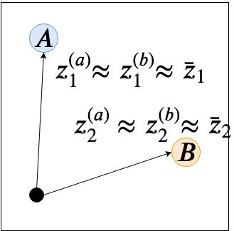
In this section our aim is to provide an intuitive explanation of why learning hard options in a multitask setting can lead to local optima and how soft options can overcome this. In this local optimum, multiple options have learned the same behavior and are unable to change it, even if doing so would ultimately lead to a higher reward. We use the Moving Bandits experiment schematically depicted in Figure 2 as an example. The agent (black dot) observes two target locations and but does not know which one is the correct one that has to be reached in order to generate a reward. The state- and action-spaces are continuous, requiring multiple actions to reach either or from the starting position. Consequently, having access to two options, one for each location, can accelerate learning. Experimental results comparing msol against a recently proposed ‘hard option’ method (Meta Learning of Shared Hierarchies (mlsh), (Frans et al., 2018)) are discussed in Section 5.1.
Let us denote the options we are learning as and and further assume that due to random initialization or late discovery of target , both skills currently reach . In this situation, the master policies on tasks in which the correct goal is are indifferent between using and and will consequently use both with equal probability.
In the case of hard options, changing one skill, e.g. , towards in order to solve tasks in which is the correct target, decreases the performance on all tasks that currently use to reach target , because for hard options the skills are shared exactly across tasks. Averaged across all tasks, this would at first decrease the overall average return, preventing any option from changing away from , leaving unreachable and training stuck in a local optimum.
To “free up” and learn a new skill reaching , all master policies need to refrain from using to reach and instead use the equally useful skill exclusively. Importantly, using soft options makes this possible. In Figures 2(b) and 2(c) we depict this schematically. The key difference is that in msol we have separate task-specific posteriors and for tasks and and soft options (for simplicity, we assume that the correct target is for task and for task ). This allows us, in a first step, to solve all tasks (Figure 2(b)): despite master policies on tasks still using posterior to reach , the other posterior can learn to reach . However, this now makes option less specialized across tasks, i.e. the prior does not agree with either posterior . Consequently, for tasks , the master policies will now strictly prefer option to reach , allowing option to specialize on only reaching , leading to the situation shown in Figure 2(c) in which both options specialize to reach different targets.
4 RELATED WORK
Most hierarchical approaches rely on proxy rewards to train the lower level components and their terminations. Some of them aim to reach pre-specified subgoals (Sutton et al., 1999), which are often found by analyzing the structure of the MDP (McGovern and Barto, 2001), previously learned policies (Tessler et al., 2017) or predictability (Harutyunyan et al., 2019). Those methods typically require knowledge, or a sufficient approximation, of the transition model, both of which are often infeasible.
Recently, several authors have proposed unsupervised training objectives for learning diverse skills based on their distinctiveness (Gregor et al., 2016). However, those approaches don’t learn termination functions and cannot guarantee that the required behavior on the downstream task is included in the set of learned skills. Hausman et al. (2018) also incorporate reward information, but do not learn termination policies and are therefore restricted to learning multiple solutions to the provided task instead of learning a decomposition of the task solutions which can be re-composed to solve new tasks.
A third usage of proxy rewards is by training lower level policies to move towards goals defined by the higher levels. When those goals are set in the original state space (Nachum et al., 2018), this approach has difficulty scaling to high dimensional state spaces like images. Setting the goals in a learned embedding space (Vezhnevets et al., 2017) can be difficult to train, though. In both cases, the temporal extension of the learned skills are set manually. On the other hand, Goyal et al. (2019) also learn a hierarchical agent, but not to transfer skills, but to find decisions states based on how much information is encoded in the latent layer.
HiREPS Daniel et al. (2012) also take an inference motivated approach to learning options. In particular Daniel et al. (2016) propose a similarly structured hierarchical policy, albeit in a single task setting. However, they do not utilize learned prior and posterior distributions, but instead use expectation maximization to iteratively infer a hierarchical policy to explain the current reward-weighted trajectory distribution.
Several previous works try to overcome the restrictive nature of options that can lead to sub-optimal solutions by allowing the higher-level actions to modulate the behavior of the lower-level policies Heess et al. (2016); Haarnoja et al. (2018). However, this significantly increases the required complexity of the higher-level policy and therefore the learning time.
The multitask- and transfer-learning setup used in this work is inspired by Thrun and Schwartz (1995) who suggests extracting options by using commonalities between solutions to multiple tasks. Prior multitask approaches often rely on additional human supervision like policy sketches (Andreas et al., 2017) or desirable sub-goals (Tessler et al., 2017) in order to learn skills which transfer well between tasks. In contrast, our work aims at finding good termination states without such supervision. Tirumala et al. (2019) investigate the use of different priors for the higher-level policy while we are focussing on learning transferrable option priors. Closest to our work is mlsh (Frans et al., 2018) which, however, shares the lower-level policies across all tasks without distinguishing between prior and posterior and does not learn termination policies. As discussed, this leads to local minima and insufficient diversity in the learned options. Similarly to us, Fox et al. (2016) differentiate between prior and posterior policies on multiple tasks and utilize a KL-divergence between them for training. However, they do not consider termination probabilities and instead only choose one option per task.
Our approach is closely related to distral (Teh et al., 2017) with which we share the multitask learning of prior and posterior policies. However, distral has no hierarchical structure and applies the same prior distribution over primitive actions, independent of the task. As a necessary hierarchical heuristic, the authors propose to also condition on the last primitive action taken. This works well when the last action is indicative of future behavior; however, in Section 5 we show several failure cases where a learned hierarchy is needed.
5 EXPERIMENTS
We conduct a series of experiments to show: i) msol trains successfully without complex training schedules like in mlsh (Frans et al., 2018), ii) msol can learn useful termination policies, iii) when learning hierarchies in a multitask setting, unlike other methods, msol successfully overcomes the local minimum of insufficient option diversity, as described in Section 3.5, iv) using soft options yields fast transfer learning while still reaching optimal performance, even on new, out-of-distribution tasks.
All architectural details and hyper-parameters can be found in the appendix. For all experiments, we first train the exploration priors and options on tasks from the available task distribution (training phase is plotted in Appendix D). Subsequently, we test how quickly we can learn new tasks from (or another distribution ).
We compare the following algorithms: msol is our proposed method that utilizes soft options both during option learning and transfer. msol (frozen) uses the soft options framework during learning to find more diverse skills, but does not allow fine-tuning the posterior sub-policies after transfer. distral (Teh et al., 2017) is a strong non-hierarchical transfer learning algorithm that also utilizes prior and posterior distributions. distral(+action) utilizes the last action as option-heuristic, that is, as additional input to the policy and prior, which works well in some tasks but fails when the last action is not sufficiently informative. Conditioning on an informative last action allows the distral prior to learn temporally correlated exploration strategies. mlsh (Frans et al., 2018) is a multitask option learning algorithm like msol, but utilizes ‘hard’ options for both learning and transfer, i.e., sub-policies that are shared exactly across tasks. It relies on fixed option durations and requires a complex training schedule between master and intra-option policies to stabilize training. We use the author’s mlsh implementation. We also compare against Option Critic (oc) (Bacon et al., 2017), which takes the task-id as additional input in order to apply it to multiple tasks.
Note that, during test time, mlsh and msol (frozen) can be fairly compared as each uses one fixed policy per skill. On the other hand, distral, distral(+action) and msol use adaptive posterior policies for each task and are consequently more expressive.
5.1 MOVING BANDITS


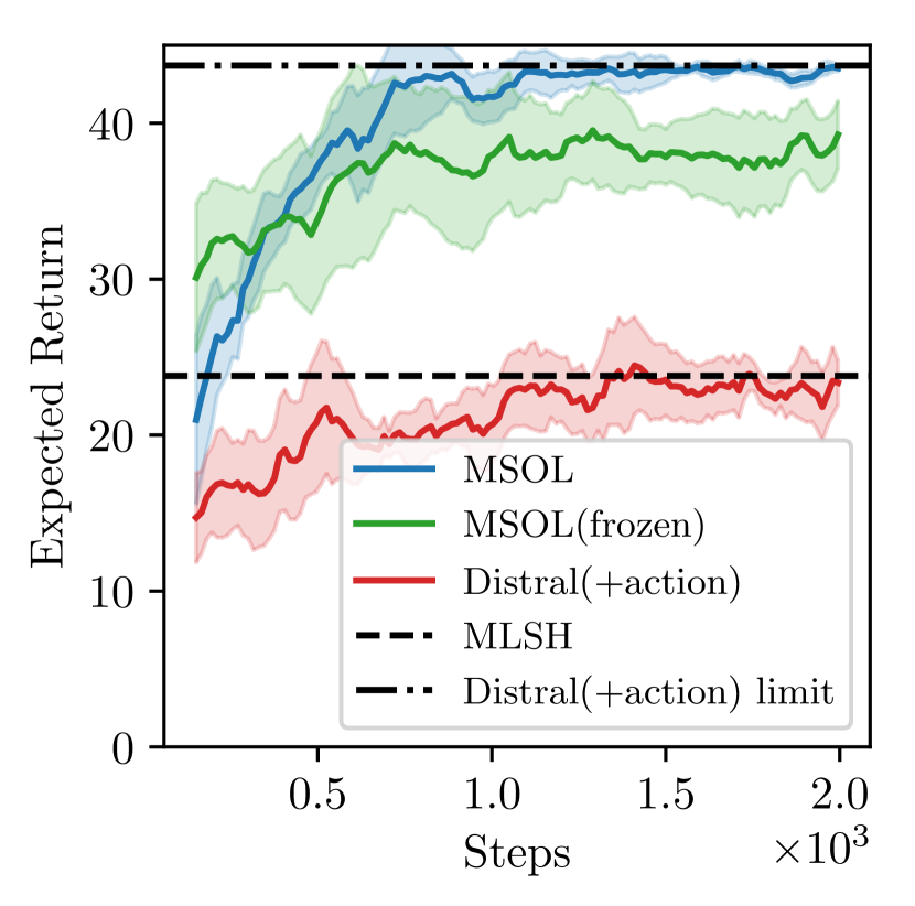
We start with the 2D Moving Bandits environment proposed and implemented by Frans et al. (2018), which is similar to the example in Section 3.5. There are two randomly sampled, distinguishable, marked positions in the environment. In each episode, the agent receives a reward of 1 for each time step it is sufficiently close to the correct one of both positions, and 0 otherwise. Which location is rewarded is not signaled in the observation. The agent can take actions that move it in one of the four cardinal directions. Each episode lasts 50 steps.
We compare against mlsh and distral to highlight challenges that arise in multitask training. We allow mlsh and msol to learn two options. During transfer, optimal performance can only be achieved with diverse options that have successfully learned to reach different marked locations. In Figure 3(a) we can see that msol is able to do so but the hard options learned by mlsh both learned to reach the same goal location, resulting in only approximately half the optimal return during transfer. This is exactly the situation outlined in Section 3.5 in which learning hard options can lead to local optima.
distral, even with the last action provided as additional input, is not able to quickly utilize the prior knowledge. The last action only conveys meaningful information when taking the goal locations into account: distral agents need to infer the intention based on the last action and the relative goal positions. While this is possible, in practice the agent was not able to do so, even with a much larger network. Much longer training ultimately allows distral to perform as well as msol, denoted by “distral(+action) limit”. This is not surprising since its posterior is flexible and will therefore eventually be able to learn any task. However, it is not able to learn transferrable prior knowledge which allows fast training on the new task. Lastly, msol (frozen) also outperforms distral(+action) and mlsh, but performs worse that msol. This highlights the utility of making options soft, i.e. adaptable, during transfer to new tasks. It also shows that the advantage of msol over the other methods lies not only in its flexibility during transfer, but also during the original learning phase.
5.2 TAXI
Next, we use a slightly modified version of the original Taxi domain (Dietterich, 1998) to show learning of termination functions as well as transfer- and generalization capabilities. To solve the task, the agent must pick up a passenger on one of four possible locations by moving to their location and executing a special ‘pickup/drop-off’ action. Then, the passenger must be dropped off at one of the other three locations, again using the same action executed at the corresponding location. The domain has a discrete state space with 30 locations arranged on a grid and a flag indicating whether the passenger was already picked up. The observation is a one-hot encoding of the discrete state, excluding passenger- and goal location. This introduces an information-asymmetry between the task-specific master policy, and the shared options, allowing them to generalize well (Galashov et al., 2019). Walls (see Figure 4) limit the movement of the agent and invalid actions.
We investigate two versions of Taxi. In the original, just called Taxi, the action space consists of one no-op, one ‘pickup/drop-off’ action and four actions to move in all cardinal directions. In Directional Taxi, we extend this setup: the agent faces in one of the cardinal directions and the available movements are to move forward or rotate either clockwise or counter-clockwise. In both environments the set of tasks are the 12 different combinations of pickup/drop-off locations. Episodes last at most 50 steps and there is a reward of 2 for delivering the passenger to its goal and a penalty of -0.1 for each time step. During training, the agent is initialized to any valid state. During testing, the agent is always initialized without the passenger on board.
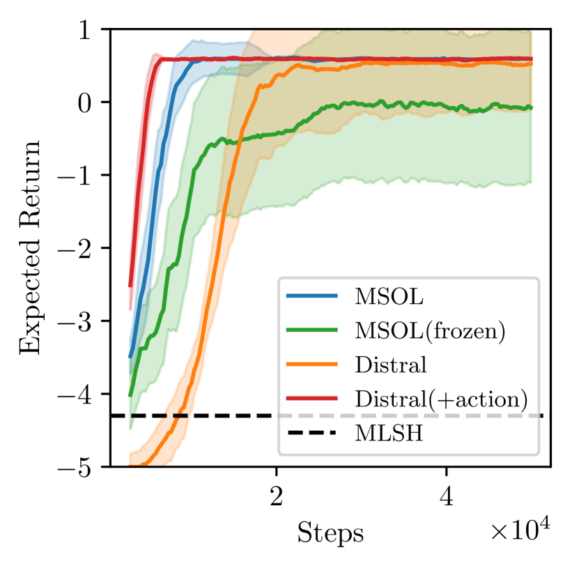
We allow four learnable options in mlsh and msol. This necessitates the options to be diverse, i.e., one option to reach each of the four pickup/drop-off locations. Importantly, it also requires the options to learn to terminate when a passenger is picked up. As one can see in Figure 3(b), mlsh struggles both with option-diversity and due to its fixed option duration: because the starting position is random, the duration until the option needs to terminate is different between episodes and cannot be captured by one hyperparameter. Furthermore, even without correct terminations, one could still learn to solve (at least) four out of the twelve tasks, leading to an average reward of approximately 222The optimal policy for a task achieves approximate a return of 0.5 on average whereas the worst possible return is .. However, mlsh is not able to learn diverse enough policies, resulting in worse performance.
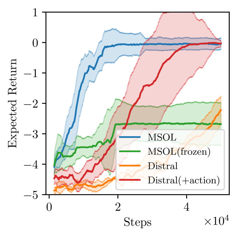
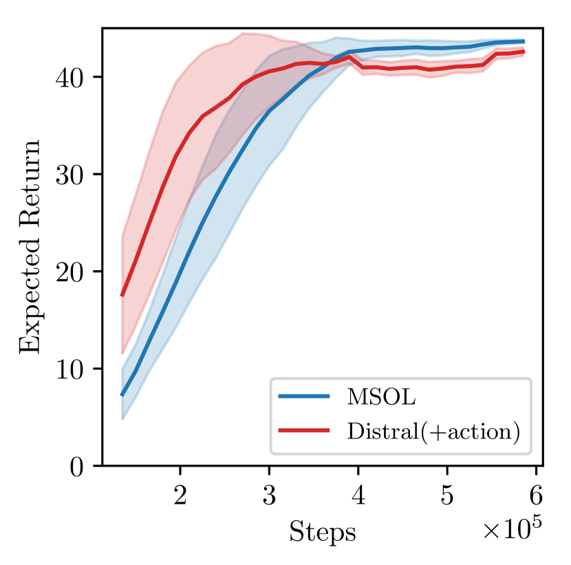
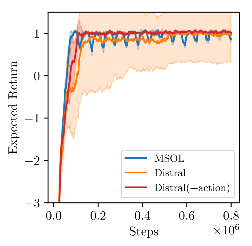
distral(+action) performs well in the original Taxi environment, as seen in Figure 3(b). This is expected since here the last action, moving in a compass direction, is a good indicator for the agent’s intention, effectively acting as an optimal “option” and inducing temporally extended exploration. However, in the directional case shown in Figure 3(c), actions rarely indicate intentions, which makes it much harder for distral(+action) to use prior knowledge. By contrast, msol performs well in both taxi environments. In the directional case, learned msol options capture temporally correlated behavior much better than the last action in distral.
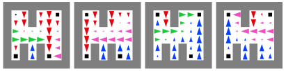
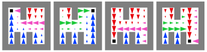
Figure 4 demonstrates that the options learned by msol learn movement and termination policies that make intuitive sense. Note that the same soft option represents different behavior depending on whether it already picked up the passenger, as this behavior does not need to terminate the current option on three of the 12 tasks.
5.3 OUT-OF-DISTRIBUTION TASKS
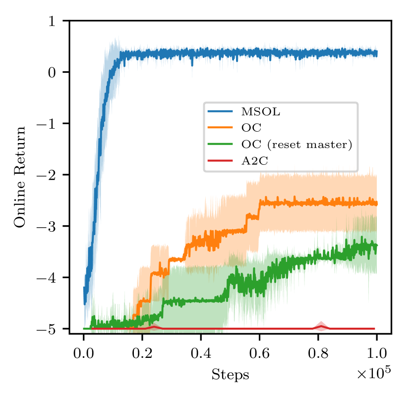
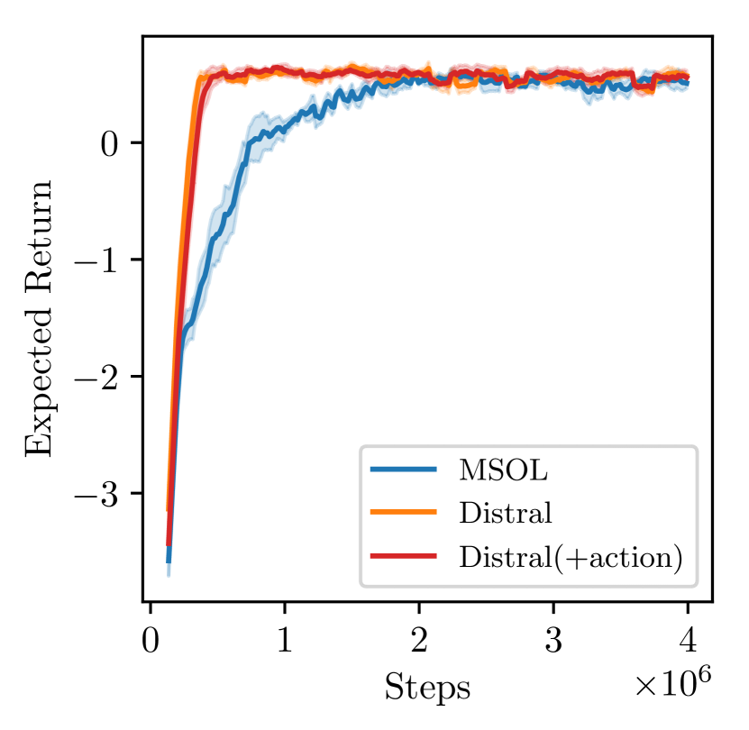
In this section, we show how learning soft options can help with transfer to unseen tasks. In Figure 5(a) we show learning on four tasks from using options that were trained on the remaining eight, comparing against Advantage Actor-critic (A2C) (Mnih et al., 2016) and Option Critic (oc) (Bacon et al., 2017). Note that in oc, there is no information-asymmetry: the same networks are shared across all tasks and provided with a task-id as additional input, including to the option-policies. This prevents oc from generalizing well to unseen tasks. On the other hand, withholding the task-information would be similar to mlsh, which we already showed to struggle with local minima. The strong performance of msol shows that information-asymmetric options help to generalize to previously unseen tasks.
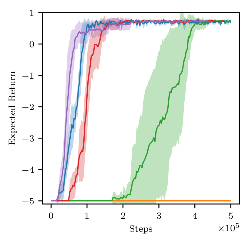
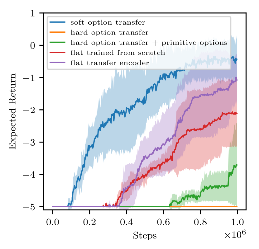
We also investigate the utility of flexible soft options under a shift of the task distribution: in Figures 5(b) and 5(c) we show learning performance on twelve modified tasks in which the pickup/dropoff locations where moved by one cell while the options were trained with the original locations. While the results in Figure 5(b) use a smaller grid, Figure 5(c) shows the results for a larger grid in which exploration is more difficult. As expected, hard options are not able to solve this task for either grid-size. Moreover, while combining hard options with primitive actions allows the tasks to be solved eventually, it performs worse than training a new, flat policy from scratch. The finding that access to misspecified, hard options can actually hurt exploration is consistent with previous literature (Jong et al., 2008). On the other hand, msol is able to quickly learn on this new task by adapting the previously learned options.
Note that on the small grid in which exploration is easy, our hierarchical method performs similar to a flat policy. On the larger grid exploration becomes more challenging and msol learns significantly faster, highlighting how transfer learning can improve exploration. More results can be found in Section D.2.
6 DISCUSSION
Multitask Soft Option Learning (msol) proposes reformulating options using the perspective of prior and posterior distributions. This offers several key advantages. First, during transfer, it allows us to distinguish between fixed, and therefore knowledge-preserving option priors, and flexible option posteriors that can adjust to the reward structure of the task at hand. This effects a similar speed-up in learning as the original options framework, while avoiding sub-optimal performance when the available options are not perfectly aligned to the task. Second, utilizing this ‘soft’ version of options in a multitask learning setup increases optimization stability and removes the need for complex training schedules. Furthermore, this framework naturally allows master policies to coordinate across tasks and avoid local minima of insufficient option diversity. It also allows for autonomously learning option-termination policies, a very challenging task which is often avoided by fixing option durations manually.
Lastly, using this formulation also allows inclusion of prior information in a principled manner without imposing too rigid a structure on the resulting hierarchy. We utilize this advantage to explicitly incorporate the bias that good options should be temporally extended. In future research, other types of information can be explored. As an example, one could investigate sets of tasks which would benefit from a learned master prior, like walking on different types of terrain.
7 ACKNOWLEDGEMENTS
MI is supported by the AIMS EPSRC CDT. NS, AG, NN were funded by ERC grants ERC-2012-AdG 321162-HELIOS and Seebibyte EP/M013774/1, and EPSRC/MURI grant EP/N019474/1. SW is supported by ERC under the Horizon 2020 research and innovation programme (grant agreement number 637713).
References
- Andreas et al. (2017) J. Andreas, D. Klein, and S. Levine. Modular multitask reinforcement learning with policy sketches. In ICML, 2017.
- Bacon et al. (2017) P.-L. Bacon, J. Harb, and D. Precup. The option-critic architecture. In AAAI, 2017.
- Bengio et al. (2009) Y. Bengio, J. Louradour, R. Collobert, and J. Weston. Curriculum learning. ACM, 2009.
- Botvinick et al. (2009) M. M. Botvinick, Y. Niv, and A. C. Barto. Hierarchically organized behavior and its neural foundations: a reinforcement learning perspective. Cognition, (3), 2009.
- Daniel et al. (2012) C. Daniel, G. Neumann, and J. Peters. Hierarchical relative entropy policy search. In Artificial Intelligence and Statistics, 2012.
- Daniel et al. (2016) C. Daniel, H. Van Hoof, J. Peters, and G. Neumann. Probabilistic inference for determining options in reinforcement learning. Machine Learning, 2016.
- Dietterich (1998) T. G. Dietterich. The MAXQ method for hierarchical reinforcement learning. In ICML, 1998.
- Fox et al. (2016) R. Fox, M. Moshkovitz, and N. Tishby. Principled option learning in markov decision processes. arXiv:1609.05524, 2016.
- Frans et al. (2018) K. Frans, J. Ho, X. Chen, P. Abbeel, and J. Schulman. Meta learning shared hierarchies. In ICLR, 2018.
- Galashov et al. (2019) A. Galashov, S. Jayakumar, L. Hasenclever, D. Tirumala, J. Schwarz, G. Desjardins, W. M. Czarnecki, Y. W. Teh, R. Pascanu, and N. Heess. Information asymmetry in KL-regularized RL. In ICLR, 2019.
- Goyal et al. (2019) A. Goyal, R. Islam, D. Strouse, Z. Ahmed, H. Larochelle, M. Botvinick, S. Levine, and Y. Bengio. Transfer and exploration via the information bottleneck. In ICLR, 2019.
- Gregor et al. (2016) K. Gregor, D. J. Rezende, and D. Wierstra. Variational intrinsic control. arXiv:1611.07507, 2016.
- Haarnoja et al. (2018) T. Haarnoja, K. Hartikainen, P. Abbeel, and S. Levine. Latent space policies for hierarchical reinforcement learning. arXiv:1804.02808, 2018.
- Harb et al. (2017) J. Harb, P.-L. Bacon, M. Klissarov, and D. Precup. When waiting is not an option: Learning options with a deliberation cost. arXiv:1709.04571, 2017.
- Harutyunyan et al. (2019) A. Harutyunyan, W. Dabney, D. Borsa, N. Heess, R. Munos, and D. Precup. The termination critic. arXiv:1902.09996, 2019.
- Hausman et al. (2018) K. Hausman, J. T. Springenberg, Z. Wang, N. Heess, and M. Riedmiller. Learning an embedding space for transferable robot skills. In ICLR, 2018.
- Heess et al. (2016) N. Heess, G. Wayne, Y. Tassa, T. Lillicrap, M. Riedmiller, and D. Silver. Learning and transfer of modulated locomotor controllers. arXiv:1610.05182, 2016.
- Jong et al. (2008) N. K. Jong, T. Hester, and P. Stone. The utility of temporal abstraction in reinforcement learning. In AAMAS. International Foundation for Autonomous Agents and Multiagent Systems, 2008.
- Levine (2018) S. Levine. Reinforcement learning and control as probabilistic inference: Tutorial and review. arXiv:1805.00909, 2018.
- McGovern and Barto (2001) A. McGovern and A. G. Barto. Automatic discovery of subgoals in reinforcement learning using diverse density. In ICML, 2001.
- Mnih et al. (2016) V. Mnih, A. P. Badia, M. Mirza, A. Graves, T. Lillicrap, T. Harley, D. Silver, and K. Kavukcuoglu. Asynchronous methods for deep reinforcement learning. In ICML, 2016.
- Nachum et al. (2018) O. Nachum, S. Gu, H. Lee, and S. Levine. Data-efficient hierarchical reinforcement learning. arXiv:1805.08296, 2018.
- Ng et al. (1999) A. Y. Ng, D. Harada, and S. Russell. Policy invariance under reward transformations: Theory and application to reward shaping. In ICML, 1999.
- Schulman et al. (2017) J. Schulman, F. Wolski, P. Dhariwal, A. Radford, and O. Klimov. Proximal policy optimization algorithms. arXiv:1707.06347, 2017.
- Sutton et al. (1999) R. S. Sutton, D. Precup, and S. Singh. Between mdps and semi-mdps: A framework for temporal abstraction in reinforcement learning. Artificial intelligence, (1-2), 1999.
- Teh et al. (2017) Y. Teh, V. Bapst, W. M. Czarnecki, J. Quan, J. Kirkpatrick, R. Hadsell, N. Heess, and R. Pascanu. Distral: Robust multitask reinforcement learning. In NeurIPS, 2017.
- Tessler et al. (2017) C. Tessler, S. Givony, T. Zahavy, D. J. Mankowitz, and S. Mannor. A deep hierarchical approach to lifelong learning in minecraft. In AAAI, 2017.
- Thrun and Schwartz (1995) S. Thrun and A. Schwartz. Finding structure in reinforcement learning. In NeurIPS, 1995.
- Tirumala et al. (2019) D. Tirumala, H. Noh, A. Galashov, L. Hasenclever, A. Ahuja, G. Wayne, R. Pascanu, Y. W. Teh, and N. Heess. Exploiting hierarchy for learning and transfer in kl-regularized rl. arXiv:1903.07438, 2019.
- Todorov (2008) E. Todorov. General duality between optimal control and estimation. IEEE, 2008.
- Vezhnevets et al. (2017) A. S. Vezhnevets, S. Osindero, T. Schaul, N. Heess, M. Jaderberg, D. Silver, and K. Kavukcuoglu. Feudal networks for hierarchical reinforcement learning. In ICML, 2017.
- Wang et al. (2016) J. X. Wang, Z. Kurth-Nelson, D. Tirumala, H. Soyer, J. Z. Leibo, R. Munos, C. Blundell, D. Kumaran, and M. Botvinick. Learning to reinforcement learn. arXiv:1611.05763, 2016.
APPENDIX
Appendix A PSEUDO CODE
Appendix B MSOL TRAINING DETAILS
B.1 OPTIMIZATION
Even though depends on , its gradient w.r.t. vanishes.333 . Consequently, we can treat the regularized reward as a classical rl reward and use any rl algorithm to find the optimal hierarchical policy parameters . In the following, we explain how to adapt A2C (Mnih et al., 2016) to soft options. The extension to PPO (Schulman et al., 2017) is straightforward.444However, for pai frameworks like ours, unlike in the original PPO implementation, the advantage function must be updated after each epoch.
The joint posterior policy in (4) depends on the current state and the previously selected option . The expected sum of regularized future rewards of task , the value function , must therefore also condition on this pair:
| (10) |
As cannot be directly observed, we approximate it with a parametrized model . The -step advantage estimation at time of trajectory is given by
| (11) |
where the superscript ‘’ indicates treating the term as a constant. The approximate value function can be optimized towards its bootstrapped -step target by minimizing . As per A2C, depending on the state (Mnih et al., 2016). The corresponding policy gradient loss is
The gradient w.r.t. the prior parameters is555Here we ignore as it is folded into later.
| (12) |
where and . To encourage exploration in all policies of the hierarchy, we also include an entropy maximization loss:
| (13) |
Note that term in (7) already encourages maximizing for the master policy, since we chose a uniform prior . As both terms serve the same purpose, we are free to drop either one of them. In our experiments, we chose to drop the term for in , which proved slightly more stable to optimize that the alternative.
We can optimize all parameters jointly with a combined loss over all tasks , based on sampled trajectories and corresponding sampled values of :
B.2 TRAINING SCHEDULE
For faster training, it is important to prevent the master policies from converging too quickly to allow sufficient updating of all options. On the other hand, a lower exploration rate leads to more clearly defined options. We consequently anneal the exploration bonus with a linear schedule during training.
Similarly, a high value of leads to better options but can prevent finding the extrinsic reward early on in training. Consequently, we increase over the course of training, also using a linear schedule.
Appendix C ARCHITECTURE
All policies and value functions share the same encoder network with two fully connected hidden layers of size 64 for the Moving Bandits environment and three hidden layers of sizes 512, 256, and 512 for the Taxi environments. Distral was tested with both model sizes on the Moving Bandits task to make sure that limited capacity is not the problem. Both models resulted in similar performance, the results shown in the paper are for the larger model. Master-policies, as well as all prior- and posterior policies and value functions consist of only one layer which takes the latent embedding produced by the encoder as input. Furthermore, the encoder is shared across tasks, allowing for much faster training since observations can be batched together.
Options are specified as an additional one-hot encoded input to the corresponding network that is passed through a single 128 dimensional fully connected layer and concatenated to the state embedding before the last hidden layer. We implement the single-column architecture of Distral as a hierarchical policy with just one option and with a modified loss function that does not include terms for the master and termination policies. Our implementation builds on the A2C/PPO implementation by, and we use the implementation for mlsh that is provided by the authors (https://github.com/openai/mlsh).
Appendix D HYPER-PARAMETERS AND ADDITIONAL ENVIRONMENT DETAILS
We use in all experiments. Furthermore, we train on all tasks from the task distribution, regularly resetting individual tasks by resetting the corresponding master and re-initializing the posterior policies. Optimizing for msol and Distral was done over . We use for Moving Bandits and Taxi.
D.1 MOVING BANDITS
For mlsh, we use the original hyper-parameters (Frans et al., 2018). The duration of each option is fixed to 10. The required warm-up duration is set to 9 and the training duration set to 1. We also use 30 parallel environments split between 10 tasks. This and the training duration are the main differences to the original paper. Originally, mlsh was trained on 120 parallel environments which we were unable to do due to hardware constraints. Training is done over 6 million frames per task.
For msol and Distral we use the same number of 10 tasks and 30 processes. The duration of options are learned and we do not require a warm-up period. We set the learning rate to and , , . Training is done over 0.6 million frames per task. For Distral we use , and also 0.6 million frames per task.
D.2 TAXI
For msol we anneal from 0.02 to 0.1 and from 0.1 to 0.05. For Distral we use . We use 3 processes per task to collect experience for a batch size of 15 per task. Training is done over 1.4 million frames per task for Taxi and 4 million frames per task for Directional Taxi. MLSH was trained on 0.6 million frames for Taxi as due to it’s long runtime of several days, using more frames was infeasible. Training was already converged.
Tasks further out of distribution
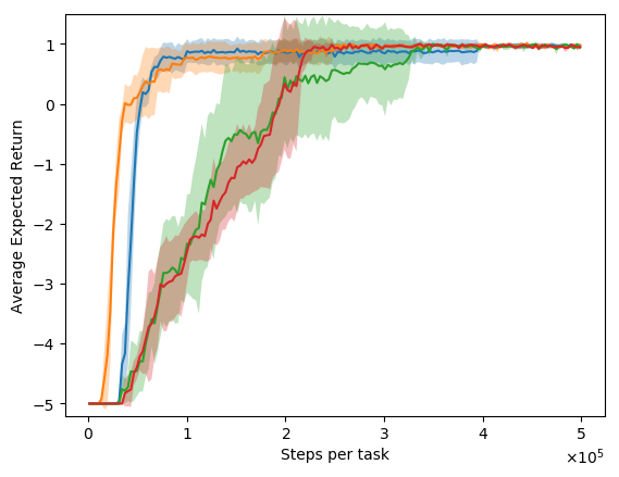
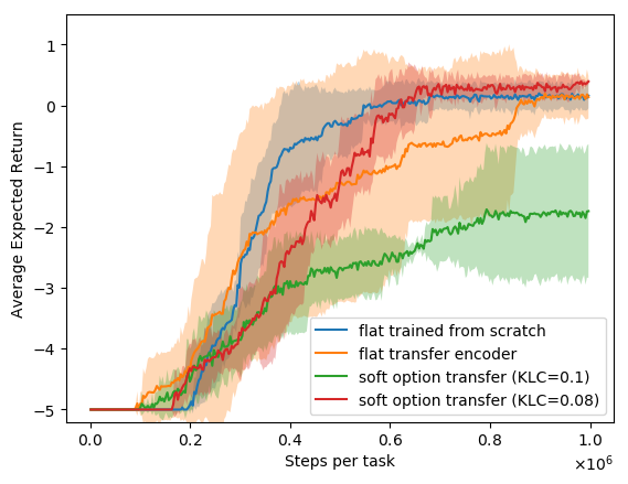
In Figure 7 we provided additional results for Section 5.3. We show the performance on further modified environments, for which the goal locations were moved by a second block from the original location for which the options were trained. We only compare soft options with flat policies trained from scratch, as we already showed in Section 5.3 that hard options are unable to cope well with goal modifications.
As expected, the flat policy trained from scratch performs similarly as before, as the moved goal location does not impact it much. On the other hand, using a pre-trained encoder performs slightly worse. On the smaller task (left figure) the options are too misspecified to be competitive, despite being soft. For the larger grid (right figure) and for a sufficienlty small value of (‘KLC’), the options, despite misspecification, are still competitive.
Consequently, while there is no hard limitation of our approach for appropriately chosen , if the target task is too different from the source task, it will be faster to learn a new policy from scratch. Which algorithm trains faster depends mainly on the difficulty of exploration in the target task. Hard exploration makes options more useful compared to a new, flat policy, even if the options are misspecified. However, the more misspecified the options are, the smaller the advantage. If target and source task are too different, very little positive transfer can be expected, and learning a new (flat) policy becomes more efficient.