Probing Primordial Chirality with Galaxy Spins

Hao-Ran Yu haoran@xmu.edu.cn Department of Astronomy, Xiamen University, Xiamen, Fujian 361005, China Canadian Institute for Theoretical Astrophysics, University of Toronto, M5S 3H8, ON, Canada Tsung-Dao Lee Institute, Shanghai Jiao Tong University, Shanghai, 200240, China Pavel Motloch Canadian Institute for Theoretical Astrophysics, University of Toronto, M5S 3H8, ON, Canada Ue-Li Pen Canadian Institute for Theoretical Astrophysics, University of Toronto, M5S 3H8, ON, Canada Tsung-Dao Lee Institute, Shanghai Jiao Tong University, Shanghai, 200240, China Dunlap Institute for Astronomy and Astrophysics, University of Toronto, M5S 3H4, ON, Canada Canadian Institute for Advanced Research, CIFAR Program in Gravitation and Cosmology, Toronto, M5G 1Z8, ON, Canada Perimeter Institute for Theoretical Physics, Waterloo, N2L 2Y5, ON, Canada Yu Yu Department of Astronomy, Shanghai Jiao Tong University, Shanghai, 200240, China Huiyuan Wang Key Laboratory for Research in Galaxies and Cosmology, Department of Astronomy, University of Science and Technology of China, Hefei, Anhui 230026, China Houjun Mo Tsinghua Center of Astrophysics & Department of Physics, Tsinghua University, Beijing, 100084, China Department of Astronomy, University of Massachusetts Amherst, MA 01003, USA Xiaohu Yang Department of Astronomy, Shanghai Jiao Tong University, Shanghai, 200240, China Tsung-Dao Lee Institute, Shanghai Jiao Tong University, Shanghai, 200240, China Yipeng Jing Department of Astronomy, Shanghai Jiao Tong University, Shanghai, 200240, China Tsung-Dao Lee Institute, Shanghai Jiao Tong University, Shanghai, 200240, China

Abstract

Chiral symmetry is maximally violated in weak interactions (1956PhRv..104..254L, ), and such microscopic asymmetries in the early Universe might leave observable imprints on astrophysical scales without violating the cosmological principle. In this Letter, we propose a helicity measurement to detect primordial chiral violation. We point out that observations of halo-galaxy angular momentum directions (spins), which are frozen in during the galaxy formation process, provide a fossil chiral observable. From the clustering mode of large scale structure of the Universe, we construct a spin mode in Lagrangian space and show in simulations that it is a good probe of halo-galaxy spins. In standard model, a strong symmetric correlation between the left and right helical components of this spin mode and galaxy spins is expected. Measurements of these correlations will be sensitive to chiral breaking, providing a direct test of chiral symmetry breaking in the early Universe.

pacs:

98.80.-k

Nature was originally considered to be simple and symmetric. Inquisitive investigations lead to the discovery of parity ( $P$ ) and charge ( $C$ ) violations in electroweak interactions (1956PhRv..104..254L, ). As chiral asymmetry exists on microscopic scales, it is interesting to ask whether the early Universe also exhibited a chiral asymmetry (1999PhRvL..83.1506L, ; 2008PhRvL.101n1101C, ; 2009PhRvL.102w1301T, ; 2016PhRvD..93k3002D, ; 2017PhRvL.118v1301M, ). If present, it might be manifested as a primordial helicity violation.

To measure certain asymmetries one needs corresponding degrees of freedom (d.o.f). At the linear order, the large scale structure of the Universe is driven by a growing mode of the scalar perturbation, which corresponds to the convergence of the velocity field and thus the growth of the density field. This clustering mode ( $E$ mode) has a single d.o.f and cannot carry any primordial chiral-helicity violations. Beyond the linear order, we may consider a primordial 3D vector field or a vector mode which can be decomposed into a scalar mode and two nonvanishing left-handed and right-handed helicity modes (supplement_1, ). However, the observation is very challenging for such a primordial vector mode because, according to the linear perturbation theory, it decays away due to the expansion of the Universe (2002PhR…367….1B, ). If we hope to observe a primordial chiral imprints at low redshifts, a nondecaying vector mode should be reconstructed to carry possibly frozen-in primordial chiral asymmetries.

Here, we construct such a primordial spin mode, a vector field written as a quadratic function of the initial tidal field that is driven by the interaction between two linear clustering modes on two different scales; the persistent $E$ mode clustering enables this spin mode growing linearly with time. This primordial spin mode well describes the vector field of angular momenta of protohalos and protogalaxies in Lagrangian space. The $E$ mode clustering then maps this field to Eulerian space. It is then possible to make a direct measurement of the primordial spin mode via observations of the rotation directions of galaxies. The spin mode has nontrivial curl and finding any asymmetry between properties of its left-handed and right-handed modes would represent a detection of primordial chiral violation.

Clustering and spin modes. — On large scales, the matter displacement field is close to being curl free and the related single d.o.f, called clustering mode or $E$ mode, well captures the inflow of matter into gravitational potential wells and ensuing increase in the density contrast (2014PhRvD..89h3515C, ; 2017PhRvD..95d3501Y, ). Many techniques can reliably estimate this $E$ mode from the late stage large scale structure and thus reconstruct the cosmic initial conditions (2014ApJ…794…94W, ; 2017PhRvD..96l3502Z, ; 2017MNRAS.469.1968P, ; 2017ApJ…847..110Y, ; 2017ApJ…841L..29W, ; 2018PhRvD..97d3502Z, ; 2019ApJ…870..116W, ). The interaction between tidal fields on different scales can cause deviation from a pure $E$ mode displacement and generate a divergence free $B$ mode.

In tidal torque theory (1984ApJ…286…38W, ), the initial angular momentum vector of a protohalo that initially occupies Lagrangian volume $V_{L}$ is approximated by $j_{\alpha}\propto\epsilon_{\alpha\beta\gamma}I_{\beta\kappa}T_{\kappa\gamma}$ , where $\mathbb{I}=(I_{\beta\kappa})$ is the moment of inertia tensor of $V_{L}$ , $\mathbb{T}=(T_{\kappa\gamma})$ is the tidal tensor acting on $\mathbb{I}$ , and $\epsilon_{\alpha\beta\gamma}$ is the Levi-Civita symbol collecting the antisymmetric components generated by the misalignment between $\mathbb{I}$ and $\mathbb{T}$ . At late times, protohalos collapse into virialized systems and their angular momentum decouples from the expansion of the Universe. The spin directions are then frozen in these systems due to the angular momentum conservation. Since $V_{L}$ represents a collection of matter that eventually clusters into a virialized system (dark matter halo), its initial collapse is driven by $\mathbb{T}$ . As a result, $\mathbb{I}$ is closely aligned with $\mathbb{T}$ (2000ApJ…532L…5L, ; 2001ApJ…555..106L, ; 2002MNRAS.332..325P, ). If they were perfectly aligned, no spin would be generated in the leading order. However, some misalignment arises from inhomogeneity of the tidal field. This motivates us to define

\boldsymbol{j}_{R}=(j_{\alpha})\propto\epsilon_{\alpha\beta\gamma}\mathcal{T}_{\beta\kappa}\mathcal{T}^{+}_{\kappa\gamma},

(1)

where $\mathbfcal{T},\mathbfcal{T}^{+}$ are tidal fields constructed as Hessians of the initial gravitational potential smoothed at two different scales $r,R$ . In what follows, we show that for properly chosen $r$ and $R$ , $\boldsymbol{j}_{R}$ is a good approximation for an angular momentum of a protohalo. To obtain $\mathbfcal{T},\mathbfcal{T}^{+}$ , we smooth the initial gravitational potential $\phi_{\rm init}({\boldsymbol{q}})$ , or its value obtained by reconstruction, by multiplying it in the Fourier space by the baryonic acoustic oscillation damping model ${\mathcal{D}}(k)^{1/4}=\exp(-r^{2}k^{2}/2)^{1/4}$ (2017PhRvD..95d3501Y, ).

Helicity decomposition. — Chirality can be violated without violating the cosmological principle (homogeneity and isotropy). In a simple analogy, sea snails could be distributed homogeneously in the sea and each of them could be oriented in a random direction, however more than 90% of their shells have right-handed whorls (Schilthuizen2005TheCE, ). The cosmic velocity and angular momentum fields could also be homogeneous and isotropic on large scales but show local scale-dependent helicities. To quantify this, a scale-dependent helicity decomposition is required. In Fourier space and for each nonzero $\boldsymbol{k}$ mode, any vector field can be decomposed into a curl free and a pure left-helical and pure right-helical components (supplement_1, ). Angle-averaged, component-wise power spectra from these $k\neq 0$ Fourier modes capture the statistics of helical asymmetries while satisfying the cosmological principle, like the angle-averaged matter power spectrum $P(k)$ .

The reconstructed spin mode $\boldsymbol{j}_{R}$ is divergence free, and can then be decomposed into the left and right helical fields,

\boldsymbol{j}_{R}=j_{R}^{L}\hat{\boldsymbol{e}}^{L}+j_{R}^{R}\hat{\boldsymbol{e}}^{R};\ \ \ \ j_{R}^{L/R}\equiv\hat{\boldsymbol{e}}^{L/R}\cdot\boldsymbol{j}_{R},

(2)

where the helical basis vectors $\hat{\boldsymbol{e}}^{L,R}$ are the eigenvectors of the curl operator. In a helically symmetric Universe, the two helicities are statistically interchangeable and the observed galaxy spins should have equal correlations to both. A primordial parity violation (e.g., initial velocity with nonzero helicity) would affect $\boldsymbol{j}_{R}^{L/R}$ unequally, which would lead to potentially observable effects.

Galaxy spins. — The angular momentum vector of galaxies $\boldsymbol{j}$ contains the magnitude $|\boldsymbol{j}|$ and direction $\hat{\boldsymbol{j}}$ . While the magnitudes have been studied extensively, they are hard to measure and not predictable. We thus consider only directions (hereafter spin) of galaxy angular momenta as a viable tracer of primordial spin mode. These parity-odd spins are observable (see discussions in (2019PhRvD..99l3532Y, , Sec.II)), and the galaxy spin field is closely related to the intrinsic alignment studies in that the minor axes of galaxies, being a parity-even observable, are potentially probing the direction of the (unoriented) line given by $\{{\hat{\boldsymbol{j}}},-\hat{\boldsymbol{j}}\}$ .

It is important to understand halo-galaxy spin connection. It is conceivable that processes like cooling and feedback can decorrelate the spin directions of galaxies and their halos. However, in many recent hydrodynamic galaxy formation simulations ((2015ApJ…812…29T, ; 2019PhRvD..99l3532Y, ) and references therein), which include various baryonic effects, we see a strong halo-galaxy spin correlation. Quantitatively, the spin correlation is expressed by $\mu=\cos\theta$ , where $\theta\in[0^{\circ},180^{\circ}]$ is the misalignment angle between halo and galaxy spins. In these galaxy formation simulations, a typical $\langle\mu\rangle$ is 0.7, much stronger than the null correlation $\langle\mu\rangle=0$ . As we do not see the halo-galaxy spin correlation erased by the baryonic effects, we focus only on spins of dark matter halos in what follows.

Refer to caption — Figure 1: The cross-correlation coefficient between the Lagrangian $\boldsymbol{j}_{q}$ (left) / Eulerian $\boldsymbol{j}_{0}$ (right) halo spins and spins reconstructed using Eq.(1) from known initial conditions $\boldsymbol{j}_{Ri}$ (top); $E$ mode reconstruction $\boldsymbol{j}_{RE}$ (bottom). Plotted as a function of the smoothing scales $r,R$ , for three halo mass bins. Darker colors show better reconstruction of halo spin.

Simulations and spin correlations.— We use numerical simulations to model a standard helically symmetric Universe and study the spin reconstruction. We study two $N$ -body simulations using the code CUBE (2018ApJS..237…24Y, ), that implements a particle-particle particle-mesh (P3M) algorithm. One simulation is characterized by a periodic box size $L=200\,{\rm Mpc}/h$ , grid number $N_{g}=768$ per dimension and a total number of dark matter particles $N_{p}=N_{g}^{3}$ , and the other by $L=100\,{\rm Mpc}/h$ , $N_{g}=400$ and $N_{p}=N_{g}^{3}$ . Both simulations assume a WMAP5 cosmology (2009ApJS..180..306D, ) and use Zel’dovich approximation (1970A&A…..5…84Z, ) to generate initial conditions at redshift $z_{i}=50$ . Their mass resolutions are close to $M_{\rm particle}\simeq 1.8\times 10^{9}\,M_{\odot}$ and $M_{\rm particle}\simeq 1.6\times 10^{9}\,M_{\odot}$ . We identify dark matter halos with at least 100 particles ( $M_{\rm halo}\gtrsim 1.8\times 10^{11}\,M_{\odot}$ and $M_{\rm halo}\gtrsim 1.6\times 10^{11}\,M_{\odot}$ ) by a spherical overdensity (SO) algorithm. We compare their spins in the Lagrangian space, $\boldsymbol{j}_{q}\propto\int_{V_{L}}(\boldsymbol{q}-\langle\boldsymbol{q}\rangle)\times(-\boldsymbol{\nabla}_{q}\phi){\mathrm{d}}^{3}\boldsymbol{q}$ , and in the Eulerian space (at redshift $z=0$ ), $\boldsymbol{j}_{0}\propto\int_{V_{E}}\rho(\boldsymbol{x})(\boldsymbol{x}-\langle\boldsymbol{x}\rangle)\times\boldsymbol{v}(\boldsymbol{x}){\mathrm{d}}^{3}\boldsymbol{x}$ , with the reconstructed spin.

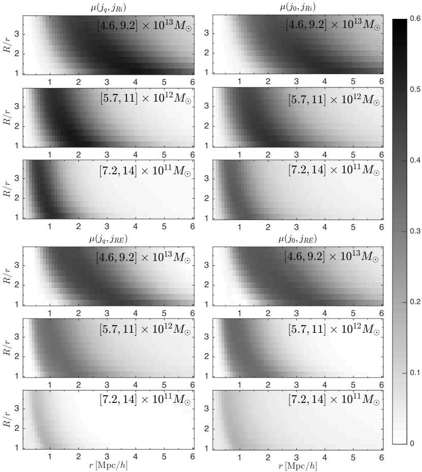
We cross-correlate the halo spins $\boldsymbol{j}_{q}$ and $\boldsymbol{j}_{0}$ with the reconstructed spin field at the Lagrangian center-of-mass of these halos $\boldsymbol{j}_{R}(\boldsymbol{q}_{h})$ . We quantify the cross-correlation of two vectors $\boldsymbol{j}_{A}$ and $\boldsymbol{j}_{B}$ by the cosine of their misalignment angle, $\mu(\boldsymbol{j}_{A},\boldsymbol{j}_{B})\equiv\boldsymbol{j}_{A}\cdot\boldsymbol{j}_{B}/|\boldsymbol{j}_{A}||\boldsymbol{j}_{B}|$ , averaged over halos in the given mass bin. In Fig.1 we show cross-correlation coefficients between four combinations of spins for a range of smoothing scales $r,R$ and halos in three mass bins. The three subpanels in the top-left quarter of Fig.1 show $\mu(\boldsymbol{j}_{q},\boldsymbol{j}_{Ri})$ , i.e., the cross-correlation between the Lagrangian spins of halos $\boldsymbol{j}_{q}$ and the spin field $\boldsymbol{j}_{Ri}$ reconstructed from the known initial conditions. We find “sweet spots” in parameter space $(r,R)$ that optimize the cross-correlation. In general, the sweet spots lay in stripes and we find that choosing $R$ close to $r$ gives the strongest correlation. As expected, for more massive halos the sweet spots shift to larger $r$ . The top-right quarter of Fig.1 shows the same, only $\boldsymbol{j}_{Ri}$ is correlated with the Eulerian spin $\boldsymbol{j}_{0}$ . The bottom part of Fig.1 then shows correlations with $\boldsymbol{j}_{RE}$ , constructed using Eq.(1) from the initial potential as determined from the $E$ mode clustering, $\phi_{E}\equiv\nabla_{q}^{-2}(-\nabla_{q}\cdot{\boldsymbol{\Psi}}({\boldsymbol{q}}))$ . As described in 2017PhRvD..95d3501Y , the $E$ mode clustering reconstruction is based on the divergence of the true displacement field ${\boldsymbol{\Psi}}$ , and represents an upper limit of how well we can reconstruct the initial conditions of the Universe when neglecting the $B$ mode portion of the displacement.

From Fig.1 we conclude that, (1) the best spin reconstruction is achieved with $R\rightarrow r_{+}$ , (2) for more massive halos, larger $r$ is preferred, (3) using $\boldsymbol{j}_{0}$ instead of $\boldsymbol{j}_{q}$ decreases the correlations only negligibly (because $\boldsymbol{j}_{q}$ is highly correlated with $\boldsymbol{j}_{0}$ ) and (4) using $\phi_{E}$ instead of the true initial potential degrades the spin reconstruction, especially for less massive halos.

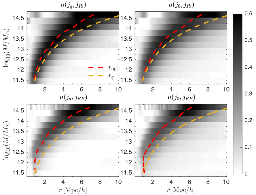
Based on the above investigations, we summarize the optimal smoothing scale as a function of halo mass in Fig.2. We chose $R\rightarrow r_{+}$ and plot $\mu$ as a function of halo mass $M$ and smoothing scale $r$ for each combination of spins from Fig.1. The red dashed curves represent the optimal smoothing scale $r_{\rm opt}$ and clearly show that $r_{\rm opt}$ increases with halo mass. For reference, we also plot the equivalent protohalo radius in the Lagrangian space $r_{q}\equiv(2MG/\Omega_{m}H_{0}^{2})^{1/3}$ ; in all cases $r_{\rm opt}$ is close to $r_{q}$ but somewhat smaller. At a given halo mass, the optimal smoothing scale $r_{\rm opt}$ is smaller for reconstruction using the $E$ mode clustering ( $\boldsymbol{j}_{RE}$ ) than for the one using the true initial conditions ( $\boldsymbol{j}_{Ri}$ ). This is probably caused by the intrinsic smoothing effect in the $E$ mode reconstruction (2017PhRvD..95d3501Y, ). Furthermore, for $\boldsymbol{j}_{RE}$ the optimal $r_{\rm opt}$ is bounded by $r_{\rm opt}\gtrsim 1\,{\rm Mpc}/h$ even for low halo masses, which indicates loss of information below this scale.

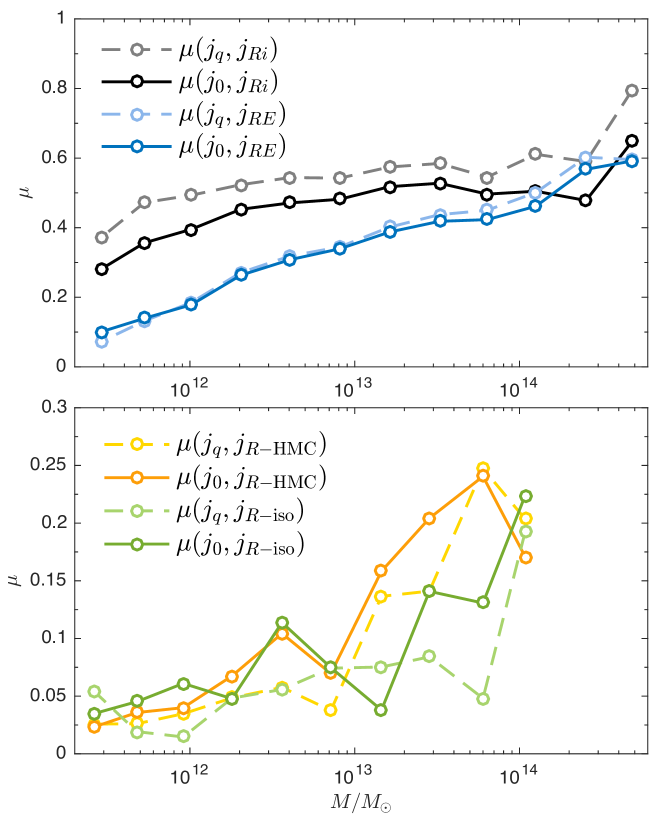
In the upper panel of Fig.3, we summarize the maximal achievable cross-correlation $\mu$ as a function of the halo mass $M$ . As expected, using the true initial conditions to reconstruct the initial spin of protohalos gives the best result. Because reconstruction based on Eq.(1) well captures the nature of spinning modes in the Lagrangian space, the correlation is high: $\mu(\boldsymbol{j}_{q},\boldsymbol{j}_{Ri})$ is close to 0.5 at halo mass $M\simeq 10^{12}M_{\odot}$ . Since for halos in mass bins above $8\times 10^{11}M_{\odot}$ we observe average $\mu(\boldsymbol{j}_{q},\boldsymbol{j}_{0})\gtrsim 0.6$ , the spins of halos are well conserved during evolution and $\mu(\boldsymbol{j}_{0},\boldsymbol{j}_{Ri})$ is comparably high. Using the $E$ mode decreases the quality of spin reconstruction for less massive halos, for which optimal reconstruction is achieved with smaller $r_{\rm opt}$ . Their spins are thus sensitive to smaller scale information, which is gradually lost in the $E$ mode reconstruction. As a result, $\mu(\boldsymbol{j}_{0},\boldsymbol{j}_{RE})$ drops below 0.2 at $M\simeq 10^{12}M_{\odot}$ .

To get a better estimate of what is realistically possible, we use the small box simulation to reconstruct the initial gravitational potential using either Hamiltonian Markov chain (HMC) reconstruction (2014ApJ…794…94W, ) or the isobaric reconstruction (2017PhRvD..96l3502Z, ; 2017MNRAS.469.1968P, ). These gravitational potentials are then used to reconstruct the initial spin field according to Eq.(1). We plot the results of spin reconstruction from HMC and isobaric density reconstructions in the lower panel of Fig.3. Because they lose even more small scale information, the spin correlations are around 0.05 $-$ 0.1 for halo masses between $10^{12}M_{\odot}$ and $10^{13}M_{\odot}$ . For both isobaric and HMC results, we find that $r_{\rm opt}\simeq 2.5\,{\rm Mpc}/h$ , which indicates that the potential fields $\phi_{\rm iso}$ and $\phi_{\rm HMC}$ contain little information below this scale and one has to use larger scale tidal field to reconstruct the spin.

Conclusion and discussion.— We considered the possibility of primordial chiral violation of the Universe. To facilitate a detection, we construct a nondecaying vector mode which is frozen in during the epoch of galaxy formation, and can be carried to the current epoch of the Universe by galaxy spins. Any primordial chiral asymmetries projected to the helical decomposition [Eq.(2)] of the spin mode can be reflected in the observed galaxy spins.

Vector modes are a combination of left and right helical mode. They can arise primordially, through second order interactions in the standard model (2009JCAP…02..023L, ), or through interactions beyond the standard model. Cosmic strings, for example, are active, causal sources of vector modes (1998PhRvD..58b3506T, ). The standard Nambu action for the equation of motion is parity symmetric, but one could envision non-Abelian helicity-violating equations of motion (1997ApJ…491L..67S, ). On scales of $\sim 1\,{\rm Mpc}$ their amplitude is very poorly constrained, and they could annihilate after imprinting helicity on the velocity field. A modified version of gravity could include a source term $\boldsymbol{F}=H\epsilon\mathbb{T}\mathbb{T}^{+}$ , where $H$ is an explicitly helicity violating operator. Such a term appears nonlocal, though no more than the nonlocality of Poisson’s equation for the Newtonian limit. We leave it for future work to consider the extension to a causal, relativistic theory with such a slow motion limit.

A measurement from survey data is beyond the scope of this Letter. The observational complexities require a thorough understanding of the systematics. The strong spin correlation between disk galaxies and their parent halos is confirmed in hydrodynamic simulations (2015ApJ…812…29T, ; 2019MNRAS.488.4801J, ), so in this Letter we use halos to represent galaxies. Strong Lagrangian-Eulerian spin correlation has also been confirmed in this work and many high-resolution $N$ -body simulations (2000ApJ…532L…5L, ; 2001ApJ…555..106L, ; 2002MNRAS.332..325P, ; 2019PhRvD..99l3532Y, ). Both of these correlations ( $\left\langle\mu\right\rangle>0.6$ ) are reliably above the null correlation $\left\langle\mu\right\rangle=0$ , indicating that neither the nonlinear effects at low redshift, nor baryonic effects during galaxy formation has washed out the primordial spin modes. For the halo-galaxy spin direction correlation $\langle\mu\rangle=0.6$ , the number of galaxies needed for a spin-correlation detection increases by only $\langle\mu\rangle^{-1}-1\simeq 67\%$ , compared to the case that galaxy spins perfectly trace the spin direction of their halos ( $\mu=1$ ).

The $E$ mode reconstruction, including complications from the bias of tracers (2017ApJ…847..110Y, ; 2017ApJ…841L..29W, ), redshift space distortions and survey masks (2018PhRvD..97d3502Z, ) has been intensively discussed in literature. ELUCID (2016ApJ…831..164W, ), state-of-the-art constrained simulation of the real Universe with all the above effects considered, can in principle be used for spin reconstruction. To compare with galaxy rotations, one needs an inverse displacement mapping from redshift space to Lagrangian space, with the uncertainties arising from redshift space distortion reconstruction and shell crossing, among other effects. The error in the estimation of parent halo mass is about a factor of 2 (1975BAAS….7..426T, ), comparable to the width of the halo mass bins used in this Letter. We find that such uncertainty in halo mass is sufficient to determine the optimal smoothing scale $r_{\rm opt}$ with good accuracy.

From simulations we have estimated that the correlation between halo spins and the corresponding prediction from estimators quadratic in the reconstructed displacement fields should be over 10%. Large samples of galaxy spins are thus expected to result in a significant detection of correlation. This opens the opportunity to test helicity violation observationally.

Two tests are amenable to observations: (1) the galaxy spin field can be decomposed into left and right helical fields, and their respective correlations with the reconstructed spin mutually compared; (2) the galaxy spin can be correlated with the left and right helical projections of the reconstructed spin. A signal in either scenario implies a primordial helical vorticity.

For a galaxy of negligible thickness, direction of its angular momentum can be deduced from the observed position angle and axis ratio. This limit is well applicable to spiral galaxies; correction for finite thickness can be applied (1984AJ…..89..758H, ). The citizen science project Galaxy Zoo (2008MNRAS.388.1686L, ) classified tens of thousands of spiral galaxies (see also (2011PhLB..699..224L, ) for an independent classification effort), which can be thus utilized to search for primordial helicity violation using the ideas presented in this work. A statistically significant preference for $S$ -wise winding galaxies in this sample was found to be a selection effect (2017MNRAS.466.3928H, ). This artificial signal contributes to the $k=0$ mode of the helicity decomposition and violates the cosmological principle. It might increase noise in the measurement but is not expected to bias the results.

Helicity is a quadratic function of spin in Fourier space (supplement_1, ), so the chiral asymmetry of field $-\boldsymbol{j}$ is the same as that of $\boldsymbol{j}$ . Intrinsic alignment of galaxies are closely related to the direction of the (unoriented) line given by $\{{\hat{\boldsymbol{j}}},-\hat{\boldsymbol{j}}\}$ and potentially also have primordial chiral violation frozen in. We leave it to future studies.

Acknowledgments.— H.R.Y., P.M. and U.L.P. acknowledge the funding from NSERC. H.R.Y. is supported by NSFC 11903021. H.Y.W. is supported by NSFC 11421303. The simulations were performed on the supercomputer at CITA.

References

(1) T. D. Lee and C. N. Yang, Physical Review 104, 254 (1956).
(2) A. Lue, L. Wang, and M. Kamionkowski, Phys. Rev. Lett.83, 1506 (1999), astro-ph/9812088.
(3) C. R. Contaldi, J. Magueijo, and L. Smolin, Phys. Rev. Lett.101, 141101 (2008), 0806.3082.
(4) T. Takahashi and J. Soda, Phys. Rev. Lett.102, 231301 (2009), 0904.0554.
(5) G. Dvali and L. Funcke, Phys. Rev. D93, 113002 (2016).
(6) K. W. Masui, U.-L. Pen, and N. Turok, Phys. Rev. Lett.118, 221301 (2017), 1702.06552.
(7) See the Supplemental Material of this Letter for the scale-dependent helicity decomposition .
(8) F. Bernardeau, S. Colombi, E. Gaztañaga, and R. Scoccimarro, Phys. Rep.367, 1 (2002), astro-ph/0112551.
(9) K. C. Chan, Phys. Rev. D89, 083515 (2014), 1309.2243.
(10) H.-R. Yu, U.-L. Pen, and H.-M. Zhu, Phys. Rev. D95, 043501 (2017), 1610.07112.
(11) H. Wang, H. J. Mo, X. Yang, Y. P. Jing, and W. P. Lin, ApJ794, 94 (2014), 1407.3451.
(12) H.-M. Zhu, Y. Yu, U.-L. Pen, X. Chen, and H.-R. Yu, Phys. Rev. D96, 123502 (2017).
(13) Q. Pan, U.-L. Pen, D. Inman, and H.-R. Yu, MNRAS469, 1968 (2017), 1611.10013.
(14) Y. Yu, H.-M. Zhu, and U.-L. Pen, ApJ847, 110 (2017).
(15) X. Wang et al., ApJ841, L29 (2017), 1703.09742.
(16) H.-M. Zhu, Y. Yu, and U.-L. Pen, Phys. Rev. D97, 043502 (2018), 1711.03218.
(17) X. Wang and U.-L. Pen, ApJ870, 116 (2019), 1807.06381.
(18) S. D. M. White, ApJ286, 38 (1984).
(19) J. Lee and U.-L. Pen, ApJ532, L5 (2000), astro-ph/9911328.
(20) J. Lee and U.-L. Pen, ApJ555, 106 (2001), astro-ph/0008135.
(21) C. Porciani, A. Dekel, and Y. Hoffman, MNRAS332, 325 (2002), astro-ph/0105123.
(22) M. Schilthuizen and A. Davison, Naturwissenschaften 92, 504 (2005).
(23) H.-R. Yu, U.-L. Pen, and X. Wang, Phys. Rev. D99, 123532 (2019), 1810.11784.
(24) A. F. Teklu et al., ApJ812, 29 (2015), 1503.03501.
(25) H.-R. Yu, U.-L. Pen, and X. Wang, The Astrophysical Journal Supplement Series 237, 24 (2018).
(26) J. Dunkley et al., ApJS180, 306 (2009), 0803.0586.
(27) Y. B. Zel’dovich, A&A5, 84 (1970).
(28) T. H.-C. Lu, K. Ananda, C. Clarkson, and R. Maartens, J. Cosmology Astropart. Phys2009, 023 (2009), 0812.1349.
(29) N. Turok, U.-L. Pen, and U. Seljak, Phys. Rev. D58, 023506 (1998), astro-ph/9706250.
(30) D. Spergel and U.-L. Pen, ApJ491, L67 (1997), astro-ph/9611198.
(31) F. Jiang et al., MNRAS488, 4801 (2019), 1804.07306.
(32) H. Wang et al., ApJ831, 164 (2016), 1608.01763.
(33) R. B. Tully, O. de Marseille, and J. R. Fisher, A New Method of Determining Distances to Galaxies, in Bulletin of the American Astronomical Society, volume 7 of BAAS, p. 426, 1975.
(34) M. P. Haynes and R. Giovanelli, AJ89, 758 (1984).
(35) K. Land et al., MNRAS388, 1686 (2008), 0803.3247.
(36) M. J. Longo, Physics Letters B 699, 224 (2011), 1104.2815.
(37) W. B. Hayes, D. Davis, and P. Silva, MNRAS466, 3928 (2017), 1610.07060.

Appendix A Supplemental Material

In this supplement, we give the details of our helicity decomposition and measurement calculation. A smooth 3D vector field can be decomposed into three helical components, based on eigenvalues of the curl ( $\nabla\times$ ) operator. In Fourier space, the corresponding eigenequation reads $i\epsilon_{\alpha\beta\gamma}k_{\beta}\tilde{u}_{\gamma}=\lambda\tilde{u}_{\alpha}$ . For $k\equiv|\boldsymbol{k}|\neq 0$ , the three eigenvalues read $\lambda^{E}=0$ and $\lambda^{L/R}=\mp k$ . Here $\lambda^{E}$ defines an $E$ -mode, non-helical, irrotational field, whereas $\lambda^{L}$ and $\lambda^{R}$ correspond to pure left-helical and pure right-helical fields. The three corresponding eigenbases $\hat{\boldsymbol{e}}^{s}(\boldsymbol{k})$ ( $s=E,L,R$ ) are orthogonal and complete.

The helical decomposition can be achieved by projecting the Fourier modes $\tilde{\boldsymbol{u}}(\boldsymbol{k})$ onto $\hat{\boldsymbol{e}}^{s}(\boldsymbol{k})$ ; the corresponding projection matrices ${\mathbb{P}}^{s}=\hat{\boldsymbol{e}}^{s}\hat{\boldsymbol{e}}^{s\dagger}$ are explicitly

	$\displaystyle{\mathbb{P}}^{E}_{\alpha\beta}$	$\displaystyle=$	$\displaystyle k_{\alpha}k_{\beta}/k^{2},$		(3)
	$\displaystyle{\mathbb{P}}^{L/R}_{\alpha\beta}$	$\displaystyle=$	$\displaystyle\frac{1}{2}\left[(\delta_{\alpha\beta}-k_{\alpha}k_{\beta}/k^{2})\pm i\epsilon_{\alpha\beta\gamma}k_{\gamma}/k\right].$		(4)

Using them, a wave packet can be decomposed as

			$\displaystyle(2\pi)^{-3}\tilde{\boldsymbol{u}}(\boldsymbol{k})e^{i\boldsymbol{k}\cdot\boldsymbol{x}}=(2\pi)^{-3}e^{i\boldsymbol{k}\cdot\boldsymbol{x}}\sum_{s}{\mathbb{P}}^{s}\tilde{\boldsymbol{u}}(\boldsymbol{k})$		(5)
		$\displaystyle=$	$\displaystyle(2\pi)^{-3}e^{i\boldsymbol{k}\cdot\boldsymbol{x}}\sum_{s}\tilde{\boldsymbol{u}}^{s}(\boldsymbol{k})=\sum_{s}{\boldsymbol{u}}^{s}(\boldsymbol{x};\boldsymbol{k}),$		(5)

where we have defined $\boldsymbol{u}^{s}(\boldsymbol{x};\boldsymbol{k})=(2\pi)^{-3}\tilde{\boldsymbol{u}}_{s}(\boldsymbol{k})e^{i\boldsymbol{k}\cdot\boldsymbol{x}}$ .

Helicity decomposition of an arbitrary vector field can be then accomplished through rewriting it as a linear combination of wave packets, which can be then individually decomposed as in (5). As a result, a general vector field $\boldsymbol{u}(\boldsymbol{x})$ can be written as $\boldsymbol{u}=\boldsymbol{u}^{E}+\boldsymbol{u}^{L}+\boldsymbol{u}^{R}$ , sum of an $E$ -mode (including the constant $k=0$ mode), $L$ -mode and an $R$ -mode field.

The helicity of a 3D vector field $\boldsymbol{u}$ inside volume $V$ is defined as $H=\int\mathcal{H}\boldsymbol{u}{\mathrm{d}}V=\int\boldsymbol{u}\cdot(\nabla\times\boldsymbol{u}){\mathrm{d}}V$ and captures the mutual orientation between a field and its vorticity. We also define $H(k)\equiv\int\mathcal{H}\boldsymbol{u}(k){\mathrm{d}}V$ the scale-dependent helicity of $\boldsymbol{u}$ on scale $k$ , where $\boldsymbol{u}(k)=\sum_{\boldsymbol{k}=|k|}\tilde{\boldsymbol{u}}(\boldsymbol{k})e^{i\boldsymbol{k}\cdot\boldsymbol{x}}$ is the collection of wave packets of wavenumber $k$ . By using Parseval’s theorem,

	$\displaystyle\int_{V}\mathcal{H}\boldsymbol{u}^{L/R}{\mathrm{d}}^{3}x=\int_{V}\boldsymbol{u}^{L/R}\cdot\left(\nabla\times\boldsymbol{u}^{L/R}\right){\mathrm{d}}^{3}x$
$\displaystyle=$	$\displaystyle\int\tilde{\boldsymbol{u}}^{L/R*}(\boldsymbol{k})\cdot\left(\mp k\tilde{\boldsymbol{u}}^{L/R}(\boldsymbol{k})\right){\mathrm{d}}^{3}k$
$\displaystyle=$	$\displaystyle\mp\int\|\tilde{\boldsymbol{u}}^{L/R}(\boldsymbol{k})\|^{2}k{\mathrm{d}}^{3}k$
$\displaystyle=$	$\displaystyle\mp\int_{0}^{\infty}P^{L/R}(k)k{\mathrm{d}}k,$	(7)

where we defined $P^{s}(k)$ the power spectrum of the helicity component $\boldsymbol{u}^{s}$ . Because $\int\mathcal{H}\boldsymbol{v}^{E}{\mathrm{d}}^{3}x=0$ and the orthogonality of the helicity decomposition (Eq.(5)) we see $H(k)=k(P^{R}(k)-P^{L}(k))$ .

The $\boldsymbol{j}_{R}({\boldsymbol{q}})$ from Eq.(1) provides a spin mode that can be determined by measuring the spin direction of galaxies/halos $\boldsymbol{j}_{\rm obs}({\boldsymbol{q}})$ . As $\boldsymbol{j}_{R}({\boldsymbol{q}})$ is divergence free¹¹1 $j_{R\alpha}\propto\epsilon_{\alpha\beta\gamma}\left(\partial_{\beta}\partial_{\kappa}\phi\right)\left(\partial_{\kappa}\partial_{\gamma}\phi^{+}\right)$ , where $\phi$ and $\phi^{+}$ are the gravitational potential smoothed on two scales to produce the tidal tensor field, and its divergence $\nabla\cdot\boldsymbol{j}_{R}=\partial_{\alpha}j_{R\alpha}\propto\partial_{\alpha}[\epsilon_{\alpha\beta\gamma}(\partial_{\beta}\partial_{\kappa}\phi)(\partial_{\kappa}\partial_{\gamma}\phi^{+})]=\epsilon_{\alpha\beta\gamma}[(\partial_{\alpha}\partial_{\beta}\partial_{\kappa}\phi)(\partial_{\kappa}\partial_{\gamma}\phi^{+})+(\partial_{\beta}\partial_{\kappa}\phi)(\partial_{\alpha}\partial_{\kappa}\partial_{\gamma}\phi^{+})]=0$ ., it can be decomposed into a left and a right helical mode $\boldsymbol{j}_{R}^{L/R}$ . The primordial asymmetry of $\boldsymbol{j}_{\rm init}^{L/R}$ is projected onto $\boldsymbol{j}_{R}^{L/R}$ and is eventually measured in the nonzero chiral asymmetry $H^{\rm obs}(k)$ of $\boldsymbol{j}_{\rm obs}^{L/R}$ . The evolution of parity violations can be schematically summarized as

\boldsymbol{j}_{\rm init}^{L/R}\xrightarrow[]{\rm projection}\boldsymbol{j}_{R}^{L/R}\xrightarrow[]{\rm evolution}\boldsymbol{j}_{\rm obs}^{L/R}.

(8)

In numerical simulations we have detected that left and right helicity components of the dark matter halo spins arising from helicity violating initial conditions (represented by helicity violating initial velocities $\boldsymbol{u}_{\rm init}$ ) have different properties, and we will present these results in a future paper.