Kitaev honeycomb models in magnetic fields: Dynamical response and hidden symmetries

Abstract

Motivated by recent reports of a field-induced intermediate phase (IP) in the antiferromagnetic honeycomb Kitaev model that may be a spin liquid whose nature is distinct from the Kitaev $\mathbb{Z}_{2}$ phase, we present a detailed numerical study on the nature and dynamical response (such as dynamical spin-structure factors and resonant inelastic x-ray scattering intensities) of this field-induced IP and neighboring phases in a family of Kitaev-based models related by hidden symmetries and duality transformations. We further show that the same field-induced IP can appear in models relevant for $\alpha$-RuCl₃, which exhibit a ferromagnetic Kitaev coupling and additional interactions. In $\alpha$-RuCl₃, the IP represents a new phase, that is likely independent from the putative field-induced (spin-liquid) phase recently reported from thermal Hall conductivity measurements.

I Introduction

In magnets with strongly frustrated interactions, quantum spin liquids can arise as exotic phases of matter that lack spontaneous symmetry-breaking down to zero temperature and feature long-range entanglement and fractionalized excitations. A prime example is the exactly solvable Kitaev model on the honeycomb lattice Kitaev (2006), which hosts a quantum spin liquid ground state of itinerant Majorana fermions that couple to a static $\mathbb{Z}_{2}$ gauge field.

Material realizations of the Kitaev model have been heavily sought after, and a mechanismJackeli and Khaliullin (2009) relying on an intricate interplay of strong electronic correlations, crystal field splitting and spin-orbit coupling has brought candidate materials such as Na₂IrO₃, various polymorphs of Li₂IrO₃, and $\alpha$-RuCl₃ to the forefront of research. However, these materials all display magnetic order at low temperatures, which is a result of additional magnetic couplings extending beyond the pure Kitaev coupling. With the goal of unravelling potential residual fractionalized excitations reminiscent of the pure Kitaev model in materials, there have been various routes to suppress the magnetic order, including the application of pressureCui et al. (2017); Biesner et al. (2018); Bastien et al. (2018); Wang et al. (2018), finite temperaturesSandilands et al. (2015); Nasu et al. (2016); Do et al. (2017) or a magnetic fieldJohnson et al. (2015); Yadav et al. (2016); Sears et al. (2017); Wolter et al. (2017); Baek et al. (2017); Wang et al. (2017a); Zheng et al. (2017); Ponomaryov et al. (2017); Banerjee et al. (2018); Hentrich et al. (2018); Kasahara et al. (2018); Janssen and Vojta (2019). For the latter case, a putative field-induced phaseBaek et al. (2017); Wang et al. (2017a); Zheng et al. (2017); Banerjee et al. (2018); Kasahara et al. (2018) in $\alpha$-RuCl₃, that lacks magnetic order, is under strong scrutiny. Here, a half-integer quantized thermal Hall conductivity was recently reportedKasahara et al. (2018) for fields tilted by $30^{\circ}$ and $45^{\circ}$ out of the honeycomb plane. Such measurements have motivated much theoretical effort to analyze both the original Kitaev model as well as models with realistic extended interactions in magnetic fields.

On the theoretical side, it is known that without a magnetic field, the pure ferromagnetic (FM) and antiferromagnetic (AFM) versions of the Kitaev model are related by a unitary transformation and thus share the same topological properties. For both coupling signs, the Kitaev spin liquid (KSL) survives under a weak magnetic field, where it becomes gapped and hosts non-Abelian anyonic excitationsKitaev (2006). The effects of a stronger field after suppressing the KSL state have however recently gained much theoretical interest due to the discovery of a field-induced intermediate phase (IP) in the AFM modelZhu et al. (2018); Gohlke et al. (2018). This phase is separated from the low-field KSL and the high-field polarized state by phase transitions and could itself be a quantum spin liquid Jiang et al. (2018); Zou and He (2018); Patel and Trivedi (2018); Hickey and Trebst (2019); Jiang et al. (2019a).

Motivated by these findings, (i) we perform a detailed analysis of the nature and dynamical response of the field-induced intermediate phase and neighboring phases in a family of Kitaev-based models related by hidden symmetries and duality transformations and, (ii) we investigate the relevance of the IP phase for real materials, in particular for $\alpha$-RuCl₃, and discuss the relation of this phase to the putative field-induced phase reported from thermal Hall conductivity measurements Kasahara et al. (2018).

The paper is organized as follows; in Section II we revise the properties of the Kitaev model and present numerical results for various dynamical response functions of the FM and AFM Kitaev model in uniform magnetic fields. This includes the dynamical spin-structure factor, which can be accessed by e.g. inelastic neutron scattering (INS) or electron spin resonance (ESR) experiments, and dynamical bond correlations, that contribute to resonant inelastic x-ray scattering (RIXS) and Raman scattering. Furthermore, we probe directly static and dynamic flux-flux correlations that appear under field. In Section III.1, by making use of duality transformations in the Kitaev model, we study the effect of generalized (non-collinear) magnetic fields. Numerically, we find that the field-induced IP of the AFM Kitaev model is highly unstable against certain non-uniform field rotations, and could manifest as a line of critical points in the parameter space of such generalized fields. In Section III.2 we discuss the relevance of the field-induced IP phase of the AFM Kitaev model for real materials. By utilizing hidden symmetries in the parameter space of extended interactions, we show that the same IP phase can appear in realistic models for $\alpha$-RuCl₃, that possess a ferromagnetic Kitaev coupling and additional interaction terms, for fields perpendicular to the honeycomb plane.

II Pure Kitaev Modelin Uniform Magnetic Fields

II.1 Introduction and definitions

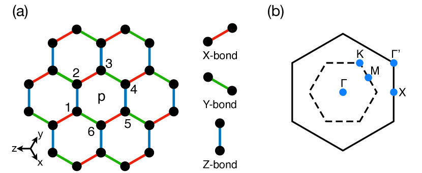
Figure 1: (a) Honeycomb lattice with definitions of cubic axes $x,y,z$ and bond types $\mathrm{X},\mathrm{Y},\mathrm{Z}$. (b) High-symmetry $k$-points in the first (dashed) and third Brillouin zone (solid border).

The Kitaev honeycomb modelKitaev (2006) is defined by a Hamiltonian consisting of bond-dependent Ising terms:

$$H_{K}=K\sum_{\braket{ij}_{\gamma}}S_{i}^{\gamma}S_{j}^{\gamma},$$ (1)

where $\gamma\in\{x,y,z\}$ corresponds to the type of bond that connects $i$ and $j$, according to Fig. 1(a).

The classical version of the model exhibits an extensive degeneracyBaskaran et al. (2008), that is lifted in the quantum model in favor of the KSL ground states. The latter can be found exactly Kitaev (2006) by representing the spins through fermionic Majorana operators $\{b_{i}^{x},b_{i}^{y},b_{i}^{z},c_{i}\}$ as $S_{i}^{\gamma}=\frac{{\mathrm{i}\mkern 1.0mu}}{2}b_{i}^{\gamma}c_{i}$. This representation introduces a $\mathbb{Z}_{2}$ gauge redundancy; physical states are spanned by unique configurations of matter fermions, and $\mathbb{Z}_{2}$ flux degrees of freedom. The latter are governed by Wilson loop operators $\{W_{L}\}$, which commute with $H_{K}$. The shortest of such loops are associated with hexagonal plaquette operators ${W}_{p}=2^{6}S_{1}^{x}S_{2}^{y}S_{3}^{z}S_{4}^{x}S_{5}^{y}S_{6}^{z}$, where the site indices refer to those in Fig. 1(a). In the ground states, the flux density

$$\braket{n_{p}}\equiv\tfrac{1}{2}\left(1-\braket{W_{p}}\right)$$ (2)

vanishes and the model can be written in terms of a free-fermion problem.

The exact solubility has facilitated a deep understanding of various response functions. The application of a single spin operator $S_{i}^{\mu}$ creates fluxes on two plaquettes, in addition to excitations in the matter sector. As a result, the dynamical spin-structure factor

$$\mathcal{S}(\mathbf{k},\omega)=\sum_{\mu=x,y,z}\int dt\ {\mathrm{e}\mkern 1.0mu}^{-{\mathrm{i}\mkern 1.0mu}\omega t}\Braket{S^{\mu}_{-\mathbf{k}}(t)\,S^{\mu}_{\mathbf{k}}(0)}$$ (3)

probes exclusively fluxful excitations, which form a continuum that is both dispersionlessBaskaran et al. (2007) and gapped, with intensity only above the two-flux gapKnolle et al. (2014a, 2015) $\Delta_{\text{f}}\simeq 0.065|K|$.

The dynamics of the bond operators $B_{ij}:=S_{i}^{\gamma}S_{j}^{\gamma}$ and of the flux operators $W_{p}$ provide further intrinsic signatures of the KSL and its field-induced phases. We consider for the bond operators the correlation function

$$\mathcal{I}_{\text{X}}(\mathbf{k},\omega):= \int dt\ {\mathrm{e}\mkern 1.0mu}^{-{\mathrm{i}\mkern 1.0mu}\omega t}\Braket{B_{-\mathbf{k}}(t)\,B_{\mathbf{k}}(0)},$$ (4)

$$B_{\mathbf{k}}:= \frac{1}{N}\sum_{i}{\mathrm{e}\mkern 1.0mu}^{{\mathrm{i}\mkern 1.0mu}\mathbf{k}\cdot\mathbf{r}_{i}}\sum_{\gamma={x,y,z}}S_{i}^{\gamma}S_{\gamma(i)}^{\gamma},$$ (5)

where $\gamma(i)$ is the nearest neighbor of $i$ along a $\gamma$-bond and $N$ is the number of sites. Due to $[B_{\mathbf{k}},W_{p}]=0$, $\mathcal{I}_{\text{X}}(\mathbf{k},\omega)$ probes only dispersive fermionic matter excitations in the flux-free sectorHalász et al. (2016), revealing gapless modes (with vanishing intensity) at $\mathbf{k}=\Gamma$ and $\mathbf{k}=\text{K}$ that reflect the Dirac spectrum of the underlying spinonsKitaev (2006). $\mathcal{I}_{\text{X}}(\mathbf{k},\omega)$ constitutes the main contribution to the spin-conserving channel of the resonant inelastic x-ray scattering (RIXS) intensityHalász et al. (2016). For $\mathbf{k}=\Gamma$, $\mathcal{I}_{\text{X}}(\Gamma,\omega)$ also contributes to Raman scatteringKnolle et al. (2014b).

Finally, we define the dynamical flux-structure factor

$$\mathcal{W}(\mathbf{k},\omega):= \ \int dt\ {\mathrm{e}\mkern 1.0mu}^{-{\mathrm{i}\mkern 1.0mu}\omega t}\Braket{W_{-\mathbf{k}}(t)\,W_{\mathbf{k}}(0)},$$ (6)

$$W_{\mathbf{k}}:= \ \frac{1}{N/2}\sum_{p}^{N/2}{\mathrm{e}\mkern 1.0mu}^{{\mathrm{i}\mkern 1.0mu}\mathbf{k}\mathbf{r}_{p}}W_{p}.$$ (7)

In the pure Kitaev model, $\mathcal{W}(\mathbf{k},\omega)$ has no intensity at finite $\omega$, reflecting that fluxes are completely static. However, generic perturbations to $H_{K}$ may lead to dynamical fluxes. In this section, we focus on the effect of a uniform magnetic field:

$$H=H_{K}-\sum_{i}\mathbf{h}\cdot\mathbf{S}_{i}$$ (8)

For weak fields, Kitaev found using perturbative arguments, that the field induces a gap in the matter fermion spectrum, which then carries a nonzero Chern numberKitaev (2006).

The fate of the model beyond this perturbative weak-field limit has been the subject of much recent interest. The FM ($K<0$) and AFM ($K>0$) versions of the Kitaev model display rather different behavior under field, which can already be anticipated on the classical level: In the case of FM coupling, a finite field instantly selects the polarized state out of the classically degenerate spin configurationsJanssen et al. (2016), suggesting a critical field of $h_{\text{c}}^{\text{FM}}=0$. For AFM coupling, the classical degeneracy is retainedJanssen et al. (2016) up to a field of $h_{\text{c}}^{\text{AFM}}=K$, as the polarized state does not fulfill the AFM spin-spin correlations preferred by the coupling. For the quantum Kitaev models (FM and AFM), the stability of the zero-field KSL is determined instead by the flux gap $\Delta_{\text{f}}$, which provides an additional emergent low energy scale. Independent of the sign of $K$, excitations carrying finite flux acquire a dispersion on the order of $h$. Suppression of the zero-field spin liquid likely occurs when this dispersion exceeds the flux gap, leading to a proliferation of fluxes at a critical field strength of $h_{\text{c}}\sim\Delta_{\text{f}}$.

This implies a finite stability of the KSL in the FM Kitaev model. Indeed, various numerical studiesJiang et al. (2011); Zhu et al. (2018); Gohlke et al. (2018); Hickey and Trebst (2019) have indicated a single phase transition as a function of field strength at $h_{\text{c}}^{\text{FM}}\approx 0.03|K|$, qualitatively independent of field directionHickey and Trebst (2019). The transition occurs directly to a quantum paramagnet (QPM) phase, that is smoothly connected to the fully polarized state of the ${h}\rightarrow\infty$ limit.

For the AFM model, the fact that $\Delta_{\text{f}}\ll K$ provides the possibility of an intermediate field regime where neither the KSL nor the polarized phase are the ground state. Consistently, recent studies have found an additional intermediate phaseZhu et al. (2018); Gohlke et al. (2018); Hickey and Trebst (2019); Jiang et al. (2018); Zou and He (2018); Patel and Trivedi (2018) (IP) for fields along the cubic $[111]$ direction (i.e. the direction perpendicular to the honeycomb plane) in the range $h_{\text{c}1}^{\text{AFM}}<h<h_{\text{c}2}^{\text{AFM}}$, with $h_{\text{c}1}^{\text{AFM}}\approx 0.4K$ and $h_{\text{c}2}^{\text{AFM}}\approx 0.6K$. The IP is thought to be gapless in the thermodynamic limitZhu et al. (2018); Gohlke et al. (2018); Hickey and Trebst (2019); Jiang et al. (2018); Zou and He (2018); Patel and Trivedi (2018). Consequently, descriptions of the IP in terms of various types of spin liquids have been proposedHickey and Trebst (2019); Jiang et al. (2018); Zou and He (2018); Patel and Trivedi (2018); Jiang et al. (2019a). Interestingly, the stability of the IP also appears to depend on the orientation of the fieldHickey and Trebst (2019); for fields along $[001]$ in the AFM Kitaev model, Majorana mean-field studiesLiang et al. (2018); Nasu et al. (2018) found a possibly different field-induced phase. In what follows, we focus on the IP that is induced for field directions including $[111]$.

II.2 Ferromagnetic Kitaev model

In order to study the phenomenology of the transition between the KSL and the field-polarized phase, we first consider the FM Kitaev model ($K<0$) in a uniform magnetic field $\mathbf{h}\parallel[111]$, described by Eq. 8. All shown results were obtained by exact diagonalization (ED) of the model on the 24-site cluster with periodic boundary conditions shown in Fig. 1(a). Other studied field directions (not shown) including $[1\bar{1}0],[11\bar{2}],$ and $[001]$ yield qualitatively similar response.

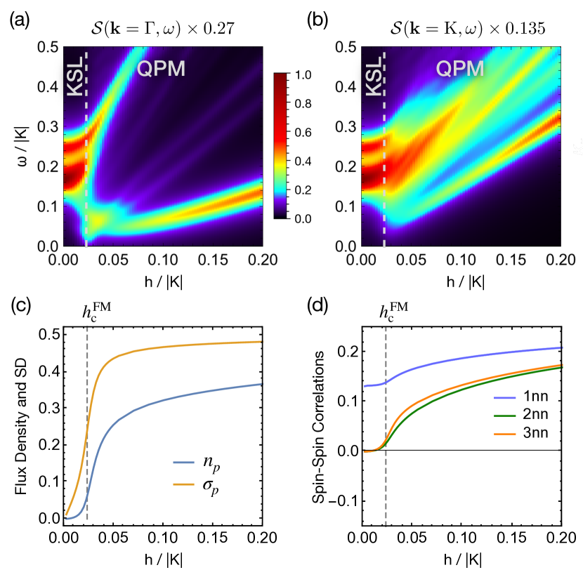
Figure 2: FM Kitaev model under $[111]$-field. (a,b) Low-frequency dynamical spin-structure factor at selected $k$-points. Poles at $\omega=0$ are not shown. (c) Flux density $\braket{n_{p}}$ and standard deviation (SD) of the local flux density $\sigma_{p}=\sqrt{\braket{{n_{p}}^{2}}-\braket{n_{p}}^{2}}$. (d) Static spin-spin correlations in real space. 1nn, 2nn, 3nn denote $\braket{\mathbf{S}_{i}\cdot\mathbf{S}_{j}}$ on first-, second- and third-nearest neighbors, respectively.

The evolution of the dynamical spin-structure factor $\mathcal{S}(\mathbf{k},\omega)$ is shown in Fig. 2(a,b) for $\mathbf{k}=\Gamma$ and K, respectively. Starting from the KSL at $h=0$, the applied field leads to broadening of the intense band of spin excitations that appear just above the two-flux gap in the range $\omega\sim 0.1-0.3\ |K|$. This broadening can be attributed to the field-induced dispersion for the fluxful excitations, which ultimately leads to the closure of the spin gap at $h_{\text{c}}^{\text{FM}}\sim 0.02|K|$. This signals a strong mixing between different flux sectors, and a breakdown of the zero-field topological order. Coming from high-field, semiclassical spin-wave approaches would suggest a softening of magnons at all wave vectors on approaching the spin liquidMcClarty et al. (2018). As a result, the spin excitation gap may close everywhere in $\mathbf{k}$-space simultaneously. For $h>h_{\text{c}}^{\text{FM}}$, the slope of the magnon energies with respect to field is smallest at $\mathbf{k}=\Gamma$ (compare Fig. 2(a) and (b)), as the minimal energy magnons exist at the zone center in the limit of large field.

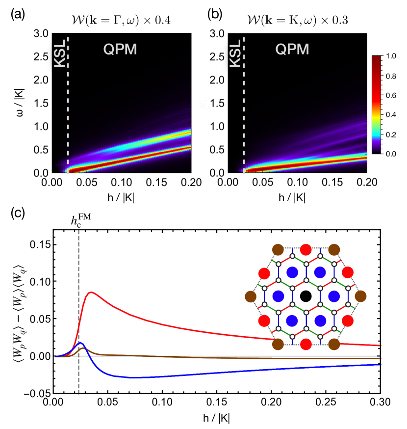
Figure 3: Flux correlations in the FM Kitaev model under $[111]$-field. (a,b) Dynamical flux-structure factor $\mathcal{W}(\mathbf{k},\omega)$. (c) $\braket{W_{p}W_{q}}-\langle{W_{p}}\rangle\langle{W_{q}}\rangle$, where each line color refers to the relative position of the respective plaquette $p$ to the black plaquette $q$ shown in the inset.

The emergence of fluxes under field can be seen in the evolution of the average flux density $\braket{n_{p}}$ shown in Fig. 2(c). While fluxes remain to be nearly absent in the KSL until the critical field $h_{\text{c}}^{\text{FM}}$, the average flux density and local flux density fluctuations measured by $\sigma_{p}=\sqrt{\braket{{n_{p}}^{2}}-\braket{n_{p}}^{2}}$ rapidly increase at the transition into the QPM. Remarkably, $\braket{n_{p}}$ stays significantly below the limit for the classical polarized state, $\lim_{h\to\infty}\braket{n_{p}}=\frac{13}{27}\simeq 0.48$, for a wide range of field strengths, implying significant quantum fluctuations in the QPM. The latter are also evident from long-range spin-spin correlations developing only gradually above $h_{\text{c}}^{\text{FM}}$, cf. Fig. 2(d).

Since $W_{p}$ commutes with $H_{K}$, the dynamics of the fluxes are mostly controlled by the field strength. In the asymptotically polarized region at high-field, the dynamical flux-structure factor $\mathcal{W}(\mathbf{k},\omega)$ (see Fig. 3(a,b) for $\mathbf{k}=\Gamma,\text{K}$ respectively) features a series of excitation bands corresponding to $n$-spin flips that do no alter $\langle S_{i}^{\gamma}S_{j}^{\gamma}\rangle$. On approaching $h_{\text{c}}^{\text{FM}}$ from above, these excitations collapse into a narrow frequency range on the scale of the zero-field flux gap $\Delta_{\text{f}}$. Importantly, since $h_{\text{c}}^{\text{FM}},\Delta_{\text{f}}\ll|K|$, the flux dynamics near the critical field are exceedingly slow compared to the time scales for other excitations. As a result, the finite flux-density state just above the critical field may be discussed in terms of nearly static fluxes, making it useful to consider the real-space static flux-flux correlations.

The static flux-flux correlations $\langle W_{p}W_{q}\rangle-\langle W_{p}\rangle\langle W_{q}\rangle$ are shown in Fig. 3(c). Deep in the KSL, the magnetic field creates virtual pairs of fluxes on neighboring plaquettes, which then may hop to adjacent plaquettes. However, flux pairs remain confined due to the finite flux gap. As a result, fluctuations around the flux-free ground state lead to positive real-space correlations that decay with increasing plaquette separation. In contrast, for $h>h_{\text{c}}^{\text{FM}}$, the correlations are markedly different, likely reflecting effective interactions between fluxes that exist in finite density. The energetics of different flux configurations was studied first by KitaevKitaev (2006), and later by Lahtinen et al.Lahtinen (2011); Lahtinen et al. (2012, 2014). In analogy with vortices in $p+{\mathrm{i}\mkern 1.0mu}p$ superconductors, each flux binds a Majorana $c$-fermionKitaev (2006); Théveniaut and Vojta (2017) under applied field. Minimizing the energy of the Majorana bound states for pairs of fluxes leads to effective flux-flux interactions, which prefer that two fluxes are located on second neighbor plaquettes parallel to a bond, for example. The correlations observed near the critical field are consistent with flux patterns that minimize these interactions. Indeed, provided that the dynamics of the fluxes remain slow compared to the $c$-fermions, the essential effects of such bound states are likely to be preserved. While the spatial range of flux-flux correlations is difficult to diagnose from finite-size calculations, we note that a state with true long-range flux order would necessarily break additional lattice symmetries, and would therefore be distinct from the fully polarized state. Since no signatures of an additional phase transition have been detectedZhu et al. (2018); Gohlke et al. (2018), it is likely that the flux-flux correlations retain a finite range in the thermodynamic limit. Therefore, the large flux-flux correlations observed in these calculations do not appear to reflect the formation of a long-range ordered flux (vison) crystal of the type studied in Ref. Zhang et al., 2019.

The fate of the matter fermions can be diagnosed from dynamical bond correlations. We therefore discuss the spin-conserving channel of the resonant inelastic x-ray scattering (RIXS) intensity $\mathcal{I}_{\text{X}}(\mathbf{k},\omega)$, as defined in Eq. 4. For completeness, we note that the form of the operator in Eq. (5) neglects additional contributions to the response that can appear at finite field related to differences in $g$-tensors between core and valence shell states. For a direct RIXS process in the first-order fast-collision approximation (employed in Ref. Halász et al., 2016), the RIXS operator gains an additional single-spin term under field, with relative magnitude $\sim\left|(\mathbf{g}_{\text{c}}-\mathbf{g}_{\text{v}})\cdot\mathbf{h}\right|/|K|$, where $\mathbf{g}_{\text{c}}$ and $\mathbf{g}_{\text{v}}$ are the $g$-tensors of the core and valence shells that are involved in the RIXS process. Under the assumption that these $g$ tensors are similar, and for fields $h$ smaller than $|K|$, the main contribution to the spin-conserving RIXS intensity should therefore still be described by $\mathcal{I}_{\text{X}}(\mathbf{k},\omega)$ under finite fields.

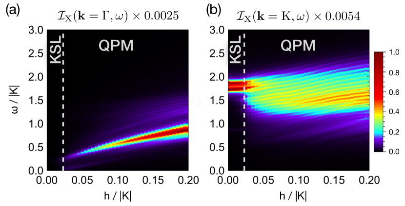
Figure 4: Spin-conserving RIXS intensity $\mathcal{I}_{\text{X}}(\mathbf{k},\omega)$ in the FM Kitaev model under $[111]$-field.

Exact diagonalization results for $\mathcal{I}_{\text{X}}(\mathbf{k},\omega)$ are shown in Fig. 4 (a) and (b) for $\mathbf{k}=\Gamma$ and K respectively. In the zero-field KSL, the majority of the spectral weight is represented by two-fermion excitations at energies $\omega\gtrsim 0.8|K|$ at all wave vectors, as in Fig. 4(b). The $\mathbf{k}$-points $\Gamma$, and $\Gamma^{\prime}$ are an exception, as the intensity vanishes at zero field due to $[B_{\mathbf{k}=\Gamma,\Gamma^{\prime}},H_{K}]=0$ (Fig. 4(a)). The discreteness of these features in our calculations can be attributed to finite size effects, but their energy range agrees with exact calculations at zero fieldHalász et al. (2016). Under finite field, the sharp excitations of the KSL significantly broaden, consistent with strong scattering from the finite density of fluxes introduced by $h$. As a result, the matter fermions cease to be well-defined excitations almost immediately upon entering the QPM phase above $h_{\text{c}}^{\text{FM}}$. In contrast to the AFM Kitaev model discussed below, the broad excitation bands, that emerge above $h_{\text{c}}^{\text{FM}}$, begin at frequencies similar to their corresponding zero-field two-fermion excitations. At high fields strengths $h\gg h_{\text{c}}^{\text{FM}}$ , the QPM can eventually be described as asymptotically polarized. Since the bond-bond correlations probe multi-spin flip excitations, they become increasingly expensive under applied field and, accordingly, the broad bands of excitations shift to higher energies with increasing $h$.

II.3 Antiferromagnetic Kitaev model

We now consider the AFM Kitaev model in uniform [111] field. To mitigate some finite-size effects in the intermediate phase, we slightly break $C_{3}$ symmetry by choosing the coupling strength on Z-bonds ($K_{z}$) stronger than that on X- and Y-bonds: $K=K_{x}=K_{y}$, $K_{z}=1.05K_{x}$. Dynamic and static response functions computed via ED are shown in Figs. 5, 6 and 7.

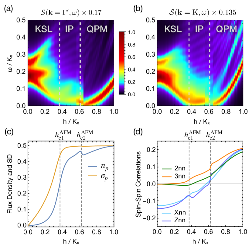
Figure 5: AFM Kitaev model with $K_{x}=K_{y},K_{z}=1.05K_{x}$ under $[111]$-field. (a,b) Low-frequency dynamical spin-structure factor. (c) Flux density $\braket{n_{p}}$ and standard deviation (SD) of the local flux density $\sigma_{p}=\sqrt{\braket{{n_{p}}^{2}}-\braket{n_{p}}^{2}}$. (d) Static spin-spin correlations in real space. Xnn and Znn denote $\braket{\mathbf{S}_{i}\cdot\mathbf{S}_{j}}$ on X- and Z-bonds, respectively.

For the dynamical spin-structure factor shown in Fig. 5(a,b) at $\mathbf{k}=\Gamma^{\prime},\text{K}$, we reproduce the results of Ref. Hickey and Trebst, 2019. At small $h$, the intense excitations at the flux gap broaden significantly, with the lower bound reaching nearly zero frequency at $h_{\text{c}1}^{\rm AFM}\approx 0.4K$. Unlike a transition to a spin-ordered phase Gotfryd et al. (2017), the spin gap appears to close everywhere in $k$-space simultaneously at $h_{\text{c}1}^{\rm AFM}$, so that clear magnetic Goldstone modes do not emerge at low frequencies. The spin gap remains small within ED resolution up to the second critical field $h_{\text{c}2}^{\rm AFM}\approx 0.6K$. This observation has previously been interpreted as the presence of gapless spin excitations in the IP in the thermodynamic limitHickey and Trebst (2019); Gohlke et al. (2018).

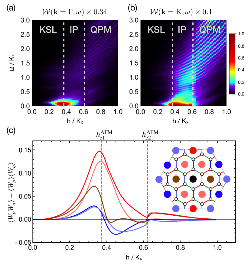
Figure 6: Flux correlations in the AFM Kitaev model with $K_{x}=K_{y},K_{z}=1.05K_{x}$ under $[111]$-field.

Similar to the FM model, the vanishing energy difference between different flux sectors at $h_{\text{c}1}^{\rm AFM}$ allows fluxes to proliferate. As a result, the first critical field marks a rapid increase in the average flux density $n_{p}$, as well as in local flux-density fluctuations $\sigma_{p}$, see Fig. 5(c). In contrast, both quantities change very little at the second critical field $h_{c2}^{\text{AFM}}$.

In the IP, the dynamical flux-structure factor $\mathcal{W}(\mathbf{k},\omega)$, shown in Fig. 6(a,b), displays a broad continuum in the energy range $\omega\sim 0$ to $3K$. However, much of the spectral weight is concentrated at small frequencies $0\lesssim\omega\lesssim 0.1K$, on the same scale as the zero-field flux gap. This indicates that the flux fluctuations—while large in amplitude $\sigma_{p}$—occur primarily on relatively slow time scales throughout the IP. This is in contrast to neighboring ordered phases of the KSL, which can be induced by e.g. an additional Heisenberg term, where we find the spectral weight of $\mathcal{W}(\mathbf{k},\omega)$ to be concentrated at higher frequencies, with negligible weight near $\omega\approx 0$. Likewise, in the QPM phase in Fig. 6(a,b) for $h>h_{\text{c}2}^{\rm AFM}$, the low-frequency intensity in $\mathcal{W}(\mathbf{k},\omega)$ is rapidly suppressed. Here, the opening of a gap at $h_{\text{c}2}^{\rm AFM}$ shifts all excitations to higher energies with increasing field. Similar to the FM model near $h_{\text{c}}^{\text{FM}}$, the IP features pronounced modulation of the static flux-flux correlations $\langle{W}_{p}{W}_{q}\rangle-\langle W_{p}\rangle\langle W_{q}\rangle$ in real space, shown in Fig. 6(c). In this case, the correlations show a stripy pattern, the orientation of which is selected by the choice of $K_{z}>K_{x},K_{y}$. These correlations are a property of the IP, and are largely suppressed upon approaching $h_{c2}^{\text{AFM}}$.

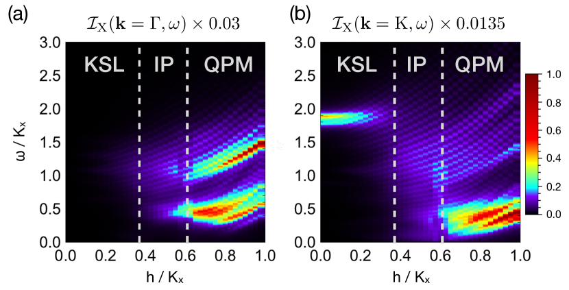
Figure 7: Spin-conserving RIXS intensity $\mathcal{I}_{\text{X}}(\mathbf{k},\omega)$ in the AFM Kitaev model with $K_{x}=K_{y},K_{z}=1.05K_{x}$ under $[111]$-field.

The spin-conserving RIXS intensity $\mathcal{I}_{\text{X}}(\mathbf{k},\omega)$ of the AFM Kitaev model under field is shown in Fig. 7. Here, the response under field differs significantly from the FM Kitaev model due to the negative sign of static bond correlations $\braket{S_{i}^{\gamma}S_{j}^{\gamma}}$ in the low-field KSL, cf. Fig. 2(d) and Fig. 5(d). Upon entering the IP at $h_{\text{c}1}^{\rm AFM}$, the discrete two-fermion excitations of the KSL observed in ED dissolve into a broad band with no distinct frequency or momentum dependence (compare Fig. Fig. 7 (a) and (b)), confirming that the $c$-fermions are strongly perturbed by the presence of the fluxes. At $h\sim h_{\text{c}1}^{\rm AFM}$, a significant portion of spectral weight in $\mathcal{I}_{\text{X}}(\mathbf{k},\omega)$ remains at high frequencies. However, in contrast to the FM model, part of the broad band shifts downward with increasing $h$, as the magnetic field reduces the energy cost for flipping the signs of $\langle S_{i}^{\gamma}S_{j}^{\gamma}\rangle$. Finally, at $h=h_{\text{c}2}^{\rm AFM}$, the band is driven to $\omega\approx 0$ at all wave vectors. Consistently, the static nearest-neighbor spin-spin correlations rapidly reverse sign upon leaving the IP, as shown in Fig. 5(d).

III Stability of the Intermediate Phase in Extended Models

III.1 Non-Collinear Fields

As discussed in Section II, the presence of the IP in the the AFM Kitaev model under a uniform field can be anticipated from two observations: (i) A finite field rapidly induces flux density fluctuations (suppressing the KSL) at $h\sim\Delta_{\text{f}}$, but (ii) does not immediately lift the extensive classical degeneracy. For this reason, a quantum spin liquid phase at intermediate fields can be anticipated. This argument can be extended to include general site-dependent fields defined by:

$$H_{\text{f}}=-\sum_{i}h_{i}^{x}S_{i}^{x}+h_{i}^{y}S_{i}^{y}+h_{i}^{z}S_{i}^{z}$$ (9)

For field configurations that do not couple to any classically degenerate state, the product of the $\gamma$-component of the local fields on all $\gamma$-bonds must satisfy

$$\text{sgn}(h_{i}^{\gamma}h_{j}^{\gamma})=\text{sgn}(K),$$ (10)

which serves as a necessary condition for the stabilization of the IP. This suggests that the IP may also be induced in the FM model for certain non-collinear field configurations satisfying $h_{i}^{\gamma}h_{j}^{\gamma}>0$. In fact, as discussed in Appendix A, the AFM Kitaev model under uniform [111] field is exactly dual to the FM model under the four-sublattice “tetrahedral” field pictured in Fig. 8. Similarly, the AFM model under the four-sublattice field is dual to the FM model under uniform [111] field.

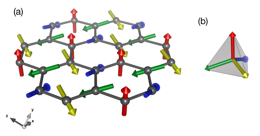
Figure 8: (a) Site-dependent directions of the four-sublattice tetrahedral field that acts on $H_{K}$ in the same way as a uniform field does on $-H_{K}$. The relative orientations of the local fields match those of the vertex corners of a tetrahedron, as shown in (b).

These dualities allow us to consider a series of models that interpolate between those possessing the IP, and those where a direct transition occurs between the KSL and the QPM. To this end, we consider the phase diagram of the AFM Kitaev model with site-dependent fields:

$$H(h,\phi)=H_{K,\text{AFM}}-h\sum_{i}\mathbf{h}_{i}(\phi)\cdot\mathbf{S}_{i},$$ (11)

with local field directions $\mathbf{h}_{i}(\phi)$ defined by the sublattice pattern in Fig. 12(d), with:

$$\mathbf{h}_{i}(\phi) =\frac{1}{\sqrt{3}}\left\{\begin{array}[]{ l l }{(1,1,1),}&{\text{if }i\in\text{sublattice A}}\\ {(v,u,v),}&{\text{if }i\in\text{sublattice B}}\\ {(v,v,u),}&{\text{if }i\in\text{sublattice C}}\\ {(u,v,v),}&{\text{if }i\in\text{sublattice D}}\end{array}\right.$$ (16)

$$u(\phi) =\cos(\phi)+\sqrt{2}\sin(\phi),$$ (17)

$$v(\phi) =\cos(\phi)-\sin(\phi)/\sqrt{2}.$$ (18)

For this choice, $\mathbf{h}_{i}(\phi)$ rotates directly between a uniform [111] field (for $\phi=0$), and the tetrahedral field shown in Fig. 8 (for $\phi=\arccos(-\frac{1}{3})\equiv\phi_{\text{tet}}\simeq 0.61\pi$). As introduced above, the model is dual to the FM Kitaev model in uniform [111] field for $\phi=\phi_{\text{tet}}$.

The phase diagram as a function of $\phi$ and $h$ obtained via ED is shown in Fig. 9(a). Phase boundaries were identified from maxima in the second derivative of the ground state energy $-\partial^{2}_{g}E_{0}$ and in the fidelity susceptibility

$$\chi_{g}=\frac{-2\log\left(\left|\langle\psi(g)|\psi(g+\delta g)\rangle\right|\right)}{(\delta g)^{2}},$$ (19)

where we have varied both $g=h$ or $g=\phi$. The locations of these maxima are shown as black points in Fig. 9(a).

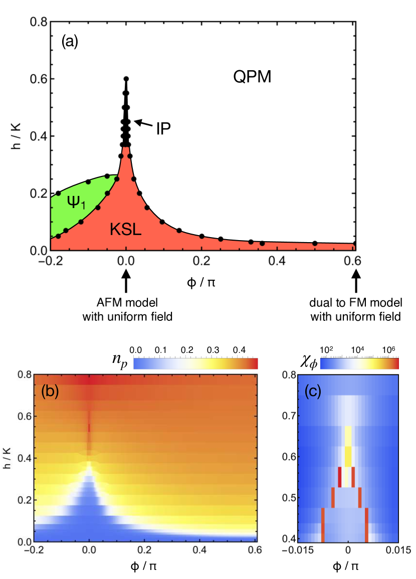
Figure 9: (a) Phase diagram interpolating between the AFM Kitaev model under a uniform $[111]$-field ($\phi=0$) and a model dual to the FM model under a uniform $[111]$-field ($\phi=\phi_{\text{tet}}\simeq 0.61\pi$) via Eqs. 11, 16, 17 and 18. Black points depict maxima in the fidelity susceptibility. (b) $\mathbb{Z}_{2}$ Flux density (Eq. 2). (c) Fidelity susceptibility (Eq. 19) with respect to $\phi$, close to the limit of uniform fields $\phi=0$. Calculated with $\delta\phi=0.005\pi$. Note that the color scale is logarithmic.

We first focus on the region for $\phi\geq 0$. As shown in the phase diagram, we find that the IP is very unstable against tetrahedral rotations, surviving only for the narrow range $\phi\lesssim 0.005\pi=0.9^{\circ}$ in our $N=24$ calculations. This is well before the necessary condition (10) for the IP stops being fulfilled at $\frac{\phi_{\text{tet}}}{2}\simeq 55^{\circ}$. For all angles $\phi>0.9^{\circ}$, a direct transition between the KSL and QPM is observed, with critical field $h_{\text{c}}$ decreasing monotonically with rotation angle. The extent of the KSL and IP can be deduced from the behavior of the flux density, plotted in Fig. 9(b). In the KSL, $n_{p}$ is suppressed, while in the IP this quantity is enhanced compared to adjacent phases. In Fig. 9(c), we show the behavior of the fidelity susceptibility $\chi_{\phi}$ in the narrow region around $\phi\sim 0$. For $0.4\lesssim\frac{h}{K}\lesssim 0.6$, the transition between the IP and the polarized phase occurs via level crossings on sweeping $\phi$, signified by two divergencies in $\chi_{\phi}$ at very small negative and positive $\phi$. For $h\gtrsim 0.6K$, the divergences meet and are rapidly suppressed.

While the above results suggest the IP has a very small—but finite—extent with respect to $\phi$, we note that the energy spectra in finite-size calculations are necessarily discrete. The level crossings shown in Fig. 9(c) can therefore not happen instantly at $\phi=0$ in our calculations, but must appear after a finitely large perturbation to the Hamiltonian. Provided that the IP is gapless in the thermodynamic limit, as concluded in Refs. Zhu et al., 2018; Gohlke et al., 2018; Hickey and Trebst, 2019; Jiang et al., 2018; Zou and He, 2018; Patel and Trivedi, 2018, the critical $\phi$ values may scale to zero as the finite-size gap closes. In our calculations on 24 sites, the narrow width of the IP is controlled by the relative scale of the energy gaps $\sim 0.01K$ between the ground state and lowest excited states at $\phi=0$. For this reason, we cannot rule out a scenario in which the IP is reduced to a line of critical points in the $(h,\phi)$ plane of Fig. 9(a) in the thermodynamic limit, with no finite extent in the $\phi$-direction. This suggests an intriguing instability with respect to tetrahedral fields. These non-uniform fields carry momenta at wave vectors $\mathbf{k}=\text{X}$. If the IP is a $\mathrm{U}(1)$ spin liquid with spinon Fermi pockets around certain momentum vectors, as proposed in Refs. Jiang et al., 2018; Zou and He, 2018; Patel and Trivedi, 2018, then the perturbing tetrahedral fields might couple states at Fermi pockets that are offset by nesting vectors $\mathbf{q}=\text{X}$, thereupon immediately opening a gap. This suggestion appears consistent with recent DMRG studies, which show a peak in the static spin structure factor at the X-points for the AFM model in [111] fields Patel and Trivedi (2018). We note that such a strong nesting would lead to Peierls-like structural instabilities if spin-lattice couplings were considered Hermanns et al. (2015).

Finally, we comment briefly on a phase detected for negative $\phi$. The region of this additional phase (named $\Psi_{1}$ in Fig. 9(a)) can be outlined clearly by maxima in $\chi_{g}$ and $-\partial_{g}^{2}E_{0}$. From the static spin-structure factor, we can not identify a dominant ordering wave vector. Within the discrete spectra of the ED calculation, the gap throughout the region of $\Psi_{1}$ is on the order of $0.02K$, so that one could speculate about a potential gaplessness in the thermodynamic limit. In this respect, it has similarities to the IP, however we do not find $\Psi_{1}$ to be smoothly connected to the IP in parameter space. Furthermore, the flux density in $\Psi_{1}$ is significantly lower than in the IP, yet still distinctly above that of the KSL, see Fig. 9(b).

III.2 Extended Interactions

To date, material realizations of Kitaev-like Hamiltonians have been sought in a number of spin-orbital coupled transition metal compounds including $\alpha$-RuCl₃, Na₂IrO₃, and various polymorphs of Li₂IrO₃. In such materials, the minimal nearest neighbor couplings can be parameterizedRau et al. (2014); Winter et al. (2016):

$$H_{JK\Gamma\Gamma^{\prime}}=\sum_{\langle ij\rangle_{\gamma}}J\ \mathbf{S}_{i}\cdot\mathbf{S}_{j}+K\ S_{i}^{\gamma}S_{j}^{\gamma}+\Gamma\ \left(S_{i}^{\alpha}S_{j}^{\beta}+S_{i}^{\beta}S_{j}^{\alpha}\right)+\Gamma^{\prime}\ \left(S_{i}^{\alpha}S_{j}^{\gamma}+S_{i}^{\gamma}S_{j}^{\alpha}+S_{i}^{\beta}S_{j}^{\gamma}+S_{i}^{\gamma}S_{j}^{\beta}\right),$$ (20)

where $\gamma\in\{x,y,z\}$ corresponds to the type of bond connecting sites $i$ and $j$, and $(\alpha,\beta,\gamma)$ is always a permutation of $(x,y,z)$. While the precise determination of magnetic Hamiltonians for the candidate materials poses an ongoing challenge, the Kitaev exchange has been shown to be of ferromagnetic type (FM, $K<0$), on grounds of the idealized microscopic mechanismJackeli and Khaliullin (2009), ab-initio studiesKatukuri et al. (2014); Yamaji et al. (2014); Kim and Kee (2016); Winter et al. (2016); Yadav et al. (2016); Wang et al. (2017b); Winter et al. (2017a); Yadav et al. (2018) and experimental analysesChaloupka and Khaliullin (2015, 2016); Do et al. (2017); Koitzsch et al. (2017); Yamauchi et al. (2018); Cookmeyer and Moore (2018); Das et al. (2019). While we have discussed in Section III.1 and Appendix A that the field-induced IP can be realized in the FM Kitaev model, this requires non-collinear and staggered fields that are unlikely to be available in real experiments. At first glance, this puts into question the relevance of the physics of the IP to real materials.

From this viewpoint, it is useful to note the presence of hidden Kitaev points in the extended $(J,K,\Gamma,\Gamma^{\prime})$-parameter space (cf. Eq. 20), which are implied by transformations discussed in Ref. Chaloupka and Khaliullin, 2015. In particular, a $\pi$-rotation of all spin-operators around the [111] axis is defined by:

$$\mathcal{R}:(\tilde{x},\tilde{y},\tilde{z})^{\intercal}=\frac{1}{3}\begin{pmatrix}-1x+2y+2z\\ +2x-1y+2z\\ +2x+2y-1z\end{pmatrix}.$$ (21)

Applying this transformation to the pure AFM Kitaev model $H_{K}$ ($K=+1$) leads to a Hamiltonian $\widetilde{H}_{K}=\mathcal{R}H_{K}\mathcal{R}^{-1}$, that is of the ($J,K,\Gamma,\Gamma^{\prime}$)-form with parameters

$$\widetilde{H}_{K}:\quad(\tilde{J},\tilde{K},\tilde{\Gamma},\tilde{\Gamma}^{\prime})=\left(+\frac{4}{9},-\frac{1}{3},+\frac{4}{9},-\frac{2}{9}\right).$$ (22)

Importantly, the signs of all anisotropic couplings (i.e. $K<0,$ $\Gamma>0$ and $\Gamma^{\prime}<0$) at this hidden AFM Kitaev point are compatible with microscopic mechanisms relevant to known Kitaev materialsRau et al. (2014); Winter et al. (2017a). Such couplings are, in principle, realizable in real materials. The static $\mathbb{Z}_{2}$ gauge field for the KSL ground state of $\widetilde{H}_{K}$ is related to new flux operators $\widetilde{W}_{p}=\mathcal{R}W_{p}\mathcal{R}^{-1}$. Since $\mathcal{R}$ commutes with the Zeeman term of a $[111]$ field, $\widetilde{H}_{K}$ hosts the IP under uniform fields. In Fig. 10, we show the position of the hidden AFM Kitaev point $\widetilde{H}_{K}$ projected into the $(J,K,\Gamma)$-parameter space.

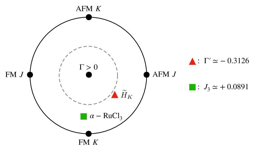
Figure 10: $(J,K,\Gamma)$-parameter space for $\Gamma>0$. We adopt the parametrization of Refs. Rau et al., 2014; Chaloupka and Khaliullin, 2015, such that $J=\sin\vartheta\cos\varphi$, $K=\sin\vartheta\sin\varphi$, $\Gamma=\cos\vartheta$, where $\varphi$ is the polar angle and $\vartheta$ is proportional to the distance from the center, reaching $\vartheta=\pi/4$ at the dashed circle and $\vartheta=\pi/2$ at the outer circle. The black dots show models where only one type of coupling is present. The triangle and the square show the projected positions of the hidden AFM Kitaev model (Eq. 22) and of the $\alpha$-RuCl₃ model (Eq. 23), respectively. Additional couplings that are not encoded in $(\varphi,\vartheta)$ are given on the right side in units of $\sqrt{J^{2}+K^{2}+\Gamma^{2}}$.

Since both the KSL and the IP at the original AFM Kitaev point have finite extents when adding additional interactions to $H_{K}$ Chaloupka et al. (2010); Rau et al. (2014); Hickey and Trebst (2019) these phases must also have finite extent around the hidden Kitaev model $\widetilde{H}_{K}$. It is therefore interesting to explore as to what extent these phases might be proximate to the phases of real materials. To that end, we take as a representative for real materials the ab-initio-guided minimal model of Ref. Winter et al., 2017b for $\alpha$-RuCl₃:

$$H_{\text{RuCl}}:\ (J,K,\Gamma,J_{3})=(-0.5,-5,+2.5,+0.5)\text{ meV},$$ (23)

where $J_{3}$ stands for third-nearest-neighbor Heisenberg coupling. We then consider models:

$$H(\xi,\mathbf{h})=(1-\xi)\,\widetilde{H}_{K}+\xi\frac{1}{C}H_{\text{RuCl}}-\sum_{i}\mathbf{h}\cdot\mathbf{S}_{i},$$ (24)

which interpolate between the hidden AFM Kitaev point ($\xi=0$) and the $\alpha$-RuCl₃ model ($\xi=1$) under uniform fields $\mathbf{h}$. We set $C=8.5\text{ meV}$ for comparable energy scales. $H_{\text{RuCl}}$ has been shown to be consistent with many experimental aspects of $\alpha$-RuCl₃ Winter et al. (2017b); Ponomaryov et al. (2017); Wolter et al. (2017); Winter et al. (2018); Riedl et al. (2018); Note (3). While the model can certainly still be further fine-tuned, we assert that the relative direction in parameter space between $\widetilde{H}_{K}$ and $\alpha$-RuCl₃ can be described reasonably well with $H_{\text{RuCl}}$.

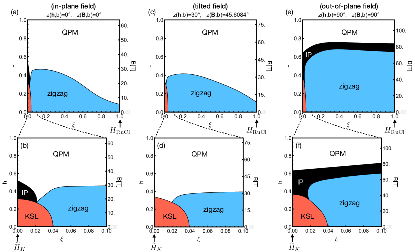
Figure 11: Phase diagrams of $H(\xi,\mathbf{h})$ from Eq. 24 for uniform fields with directions between $b=[1\bar{1}0]$ (in-plane) and $c^{*}=[111]$ (out-of-plane). $\xi=0$ corresponds to the hidden AFM Kitaev point $\widetilde{H}_{K}$ of Eq. 22, and $\xi=1$ to the $\alpha$-RuCl₃ model $H_{\text{RuCl}}$. The labels on the left axes show the energy scale of the Zeeman term as it enters Eq. 24. The labels on the right axes show the corresponding external field strengths $B=C\mu_{\text{B}}^{-1}|\mathbf{g}^{-1}\mathbf{h}|$ in Tesla, when converting to the energy scale of $\alpha$-RuCl₃ and assuming the anisotropic $g$ tensor $\mathbf{g}$ of Ref. Winter et al., 2018. Phase boundaries are determined by peaks in $\partial^{2}_{g}E_{0}$ and in $\chi_{g}$. The quantum paramagnetic (QPM) phase is smoothly connected to the fully polarized state of the $h\rightarrow\infty$ limit. (a,b) Field along $[1\bar{1}0]$, which corresponds to the crystallographic $b$ axis of $\alpha$-RuCl₃. (c,d) $\mathbf{h}$ tilted from $b$ towards $[111]=c^{*}$ by $30^{\circ}$. Assuming the mentioned $g$ tensor, this corresponds to an external $B$-field tilted by $\sim 45^{\circ}$. (e,f) $\mathbf{h}\parallel[111]=c^{*}$.

In Fig. 11 (a-f), we show the ground state phase diagrams of $H(\xi,\mathbf{h})$ for three different directions of $\mathbf{h}$, going from in-plane ($\mathbf{h}\parallel b=[1\bar{1}0]$) to out-of-plane ($\mathbf{h}\parallel c^{*}=[111]$) fields. Phase boundaries were determined from ED on the high-symmetry 24-site cluster, by tracking maxima in $\chi_{g}$ (Eq. 19) and in $-\partial^{2}_{g}E_{0}$ with $g=h$ or $g=\xi$. The physical $B$-field in Tesla is related to our natural units as $\mathbf{B}=C\mu_{\text{B}}^{-1}\mathbf{g}^{-1}\mathbf{h}$, shown on the right-hand axes in Fig. 11 for the $g$-tensor estimate of Ref. Winter et al., 2018.

On the described path through parameter space, the zigzag phase of $H_{\text{RuCl}}$ is found to be a (direct) neighbor of the hidden KSL phase, meeting it at $\xi\simeq 0.04$ for $h=0$. With increasing field strength, this phase boundary bends towards smaller $\xi$, see Figs. 11(b,d,f). Hence, no model exists on the path where an external field can suppress zigzag order in favor of a field-induced KSL state, unlike the path considered in Ref. Gordon et al., 2019, where the KSL can be field-induced for field directions close to $[111]$. For the models considered here, the stability of the KSL region is found to be qualitatively independent of field direction.

In contrast, the stability of the field-induced IP depends crucially on the field direction. Even for $\xi=0$ at the pure (hidden) Kitaev model, the IP is not induced by uniform fields near to a cubic axis (e.g. [100]), as is the case for the direction shown in Fig. 11(c,d). For most field directions where the IP is observed, it is found to be less stable than the KSL against additional interactions introduced by a finite $\xi$, as in Fig. 11(a,b), so that it cannot generally be field-induced from a zigzag ground state either. Remarkably, however, we find exclusively for the out-of-plane field-direction $[111]=c^{*}$, that the IP extends far through parameter space, reaching even the $H_{\text{RuCl}}$ model at $\xi=1$ at high fields, see Fig. 11(e,f). This result applies only for fields very near to the [111] direction. Upon rotating $\mathbf{h}$ by small angles of $\lesssim 10^{\circ}$ away from $[111]$, the extended region shrinks quickly, such that the extent of the IP with respect to $\xi$ becomes qualitatively similar to that in Fig. 11(b).

The peculiarity of the $[111]$ field direction for the stabilization of a field-induced phase in models with zigzag order hints at importance of maintaining $C_{3}$ symmetry. It may be worth noting, provided that $C_{3}$ symmetry is maintained, that a direct continuous transition between the zigzag and polarized phases is unlikely to occur in the thermodynamic limit. This is because the symmetry group of the broken symmetry zigzag ordered phase is not a maximal subgroup of the higher symmetry polarized stateAscher and Kobayashi (1977); Ascher (1977). As a result, the field-induced transition is likely to be either first order (as observed for the classical modelJanssen et al. (2017) at $\xi=1$), or feature one or more intermediate phases (as observed for zigzag phases in the classical Kitaev-Heisenberg model Janssen et al. (2016)). In finite-size calculations on the quantum modelHickey and Trebst (2019); Jiang et al. (2019b) however, the field-induced IP appears to lack long-range magnetic order, and therefore is inconsistent with either scenario observed in the classical limit. Finally, we remark the presence of level crossings between quasi-degenerate states within the IP region on the high-symmetry cluster for $[111]$ fieldsNote (2). These are expected to be inconsequential finite-size artifacts, since similar features in the nearest-neighbor Kitaev-Heisenberg vanish on larger clusters accessible by density-matrix renormalization group (DMRG) methodsJiang et al. (2019b).

Our results indicate that the IP in $\alpha$-RuCl₃ is only present for strictly out-of-plane [111] fields. This is likely a separate phase that is not necessarily linked to the various unconventional experimental observations in $\alpha$-RuCl₃ for fields tilted significantly away from $[111]$ and in-plane fields that have been interpreted in terms of a field-induced quantum spin liquidBaek et al. (2017); Wang et al. (2017a); Zheng et al. (2017); Banerjee et al. (2018); Kasahara et al. (2018).

IV Summary

In this work, we performed a detailed numerical study on the nature and dynamical response of field-induced phases in a family of Kitaev-based models related by hidden symmetries and duality transformations. Via exact diagonalization we investigated dynamical spin-structure factors—relevant in INS and ESR experiments—, dynamical bond correlations—relevant for RIXS and Raman scattering measurements—as well as dynamical flux-flux correlations.

Our results indicate that in both FM and AFM Kitaev models, the first transition where the KSL is suppressed occurs at sufficiently low fields that the dynamical timescale of the fluxes is likely to be small compared to the timescales associated with the matter fermion dynamics. As a result, the phase transition is essentially a large increase of the local flux density. The fluxes appear to experience effective interactions that are consistent with the expected features of $c$-fermion-mediated couplings.

We further find that the emergence of a field-induced intermediate phase (IP) in the AFM Kitaev model is deeply connected to the separation of energy scales between $K$ and the two-flux gap $\Delta_{\text{f}}$ and this IP phase appears in the Kitaev model for an extensive number of general non-collinear fields for both FM and AFM signs of the interaction. However, this phase is remarkably unstable against certain perturbations, specifically, a magnetic field with $\mathbf{q}=\text{X}$ momenta. This may provide clues to its identity. We also detected additional field-induced phases ($\Psi_{1}$) emerging from specific combinations of perturbations, which might be of future interest.

Finally, we demonstrated that analogues of the AFM KSL and field-induced IP phase can be found, in principle, for models with additional interactions at hidden Kitaev points under uniform fields. In particular, the IP extends in a finite region of interaction parameter space for out-of-plane fields ($\mathbf{h}\parallel[111]$), such that it can be induced in models with zigzag order, including the ab-initio-guided model for $\alpha$-RuCl₃. For $\alpha$-RuCl₃ our results predict that the IP is present for strictly out-of-plane [111] fields. This IP phase is therefore not likely linked to the putative field-induced phase recently reported in $\alpha$-RuCl₃ for fields tilted significantly away from $[111]$.

Appendix A Symmetries and Dualities at Zero and Finite Fields

In this appendix, we review the construction of general symmetries of the Kitaev model. An important feature of the Kitaev Hamiltonian at zero field is the existence of a macroscopic number of mutually commuting Wilson loop operators $\{W_{L}\}$ that also commute with ${H}_{K}$. On a torus, any combination of loops $\{L\}$ can be constructed as products of plaquette operators $\{{W}_{p}\}$ and large loop operators running around the periodic boundaries, i.e. ${W}_{L}={W}_{p_{1}}{W}_{p_{2}}...{W}_{p_{n}}$. Together, such loop operators form the generators for local symmetry transformations ${\mathrm{e}\mkern 1.0mu}^{\frac{{\mathrm{i}\mkern 1.0mu}}{2}\alpha W_{L}}{H}_{K}{\mathrm{e}\mkern 1.0mu}^{-\frac{{\mathrm{i}\mkern 1.0mu}}{2}\alpha W_{L}}=H_{K}$ with $0\leq\alpha<2\pi$. For a Hamiltonian ${H}={H}_{K}+H_{1}$, all perturbations ${H_{1}}^{\prime}={\mathrm{e}\mkern 1.0mu}^{\frac{{\mathrm{i}\mkern 1.0mu}}{2}\alpha W_{L}}{H_{1}}_{K}{\mathrm{e}\mkern 1.0mu}^{-\frac{{\mathrm{i}\mkern 1.0mu}}{2}\alpha W_{L}}$ are formally equivalent to $H_{1}$ for all $L$ and $\alpha$. For our purpose, we focus on the specific case $\alpha=\pi$, for which spin operators $\mathcal{O}=S_{i}^{\mu}S_{j}^{\nu}S_{k}^{\rho}\dots$ transform as $\mathcal{O}^{\prime}=\pm\mathcal{O}$, depending on whether they commute ($+$) or anticommute ($-$) with ${W}_{L}$. The honeycomb lattice is thus divided into four sublattices, according to the transformation associated with each site:

$$W_{L}:(x^{\prime},y^{\prime},z^{\prime})=\left\{\begin{array}[]{cc}(x,y,z),&\text{sublattice A}\\ (x,-y,-z),&\text{sublattice B}\\ (-x,y,-z),&\text{sublattice C}\\ (-x,-y,z),&\text{sublattice D}\end{array}\right.$$ (29)

Transformations generated by specific loop operators ${W}_{L}$ are shown in Fig. 12 (a-d). A specific example, shown in Fig. 12(d), is the “Klein” transformation employed in Refs. Chaloupka et al., 2010, 2013; Chaloupka and Khaliullin, 2015, which is associated to the operator $W_{\text{Klein}}$ given by the product of plaquette operators on $\tfrac{1}{4}$ of the hexagonal plaquettes (Fig. 12(c)). As noted above, the pure Kitaev Hamiltonian is mapped to itself by all such transformations, preserving the sign of the coupling ($K^{\prime}=K$). However, the operators associated with a magnetic field generally do not commute with $W_{L}$. Let us consider a general field term described by:

$$H_{\text{f}}=-\sum_{i}h_{i}^{x}S_{i}^{x}+h_{i}^{y}S_{i}^{y}+h_{i}^{z}S_{i}^{z}$$ (30)

where $h_{i}^{\mu}$ may take different values at each site. The equivalency of all combinations of local fields $W_{L}H_{\text{f}}W_{L}$ generated by different $L$ has several consequences.

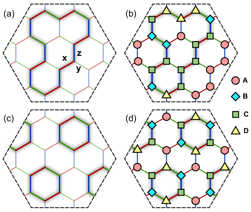
Figure 12: Construction of general four-sublattice symmetry transformations for the Kitaev model with $\alpha=\pi$. (a) Example of a loop $L$. The associated operator $W_{L}$ generates the symmetry transformation shown in (b). The specific operator $W_{\text{Klein}}$ depicted in (c) leads to the “Klein” transformation (d) employed in Refs. Chaloupka et al., 2010, 2013; Chaloupka and Khaliullin, 2015.

In Section II, we discussed the appearance of the gapless IP in the AFM Kitaev model for uniform [111] fields $H_{\text{f}}=H_{[111]}$, where $h_{i}^{x}=h_{i}^{y}=h_{i}^{z}=h$. By symmetry, equivalent states are also induced by all non-uniform field configurations described by $W_{L}H_{[111]}W_{L}$. For all such fields, the product of $\gamma$-components of the local fields on a $\gamma$-bond is positive, i.e. $h_{i}^{\gamma}h_{j}^{\gamma}>0$. Since all IP states appearing for $H=H_{K}+W_{L}H_{[111]}W_{L}$ are smoothly connected by continuous unitary transformations, they belong to a common intermediate-field phase. However these transformations do not commute with the spin operators, so that the dynamical spin-structure factor $\mathcal{S}(\mathbf{k},\omega)$ does not provide a unique characterization of the common IP. In contrast, $S_{i}^{\gamma}S_{j}^{\gamma}$ and $W_{p}$ commute with all $W_{L}$, and therefore $\mathcal{I}_{\text{X}}(\mathbf{k},\omega)$ and $\mathcal{W}(\mathbf{k},\omega)$ reflect more intrinsic characteristics that are common across all equivalent IP states.

A similar approach can be used to establish correspondence between the FM and AFM Kitaev models. We define $P_{3}$, which permutes the spin components $(x,y,z)\to(y,z,x)$ on every site. Combining this with the operator $W_{\text{Klein}}$ (see Fig. 12(c)) leads to $\mathcal{G}\equiv{\mathrm{e}\mkern 1.0mu}^{\frac{{\mathrm{i}\mkern 1.0mu}}{2}\pi P_{3}^{-1}W_{\text{Klein}}P_{3}}$, that commutes with all $W_{p}$, but anticommutes with all bond operators $S_{i}^{\gamma}S_{j}^{\gamma}$. As a result, $\mathcal{G}H_{K}\mathcal{G}^{-1}=-H_{K}$, providing a duality transformation that relates the AFM and FM Kitaev models at zero field (i.e $K^{\prime}=-K$). The transformation in real space is:

$$\mathcal{G}:(x^{\prime},y^{\prime},z^{\prime})=\left\{\begin{array}[]{cc}(x,y,z),&\text{sublattice A}\\ (-x,y,-z),&\text{sublattice B}\\ (-x,-y,z),&\text{sublattice C}\\ (x,-y,-z),&\text{sublattice D}\end{array}\right.$$ (35)

with the sublattice pattern shown in Fig. 12(d). Under the transformation $\mathcal{G}$, a uniform [111]-field $H_{[111]}$ becomes a four-sublattice “tetrahedral” field $\mathcal{G}H_{[111]}\mathcal{G}^{-1}$, with local fields $\mathbf{h}_{i}$ oriented along the [111], $[\bar{1}1\bar{1}]$, $[1\bar{1}\bar{1}]$, or $[\bar{1}\bar{1}1]$ directions as shown in Fig. 8.

If this tetrahedral field is applied to the AFM Kitaev model, it acts as a uniform field in the FM model; the tetrahedral field directly couples to one of the classically degenerate states and opens a gap immediately after the suppression of the KSL. Conversely, if the tetrahedral field is applied to the FM Kitaev model, it acts as a uniform field in the AFM model, yielding a gapless intermediate phase. This IP in the FM Kitaev model is continuously connected to the IP of the AFM Kitaev model via the unitary transformation $\mathcal{G}$, and therefore represents the same phase. For field configurations that are dual to one another, the FM model displays precisely identical dynamical flux-flux and bond-bond correlations to those observed in the AFM model. This follows from the fact that $\mathcal{G}$ commutes with $W_{p}$ and anticommutes with $S_{i}^{\gamma}S_{j}^{\gamma}$.

We remark that for all (uniform and non-uniform) fields considered here, fields that suppress the IP in the FM ($K<0$) or the AFM model ($K>0$) satisfy $\text{sgn}(h_{i}^{\gamma}h_{j}^{\gamma})\neq\text{sgn}(K)$ on all $\gamma$-bonds, while conversely fields that induce the IP satisfy on all $\gamma$-bonds

$$\text{sgn}(h_{i}^{\gamma}h_{j}^{\gamma})=\text{sgn}(K).$$ (36)

Equation 36 therefore appears to pose a necessary condition for the stability of the IP in both Kitaev models. It leads to opposing signs of nearest-neighbor spin-spin correlations $\braket{S_{i}^{\gamma}S_{j}^{\gamma}}$ between the low- and high-field limits, and thus provides an additional energy scale where the correlations reverse sign, as seen in Fig. 5(d).

References

- Kitaev (2006) A. Kitaev, Annals of Physics 321, 2 (2006).
- Jackeli and Khaliullin (2009) G. Jackeli and G. Khaliullin, Physical Review Letters 102, 017205 (2009).
- Cui et al. (2017) Y. Cui, J. Zheng, K. Ran, J. Wen, Z.-X. Liu, B. Liu, W. Guo, and W. Yu, Physical Review B 96, 205147 (2017).
- Biesner et al. (2018) T. Biesner, S. Biswas, W. Li, Y. Saito, A. Pustogow, M. Altmeyer, A. U. B. Wolter, B. Büchner, M. Roslova, T. Doert, S. M. Winter, R. Valentí, and M. Dressel, Physical Review B 97, 220401 (2018).
- Bastien et al. (2018) G. Bastien, G. Garbarino, R. Yadav, F. J. Martinez-Casado, R. Beltrán Rodríguez, Q. Stahl, M. Kusch, S. P. Limandri, R. Ray, P. Lampen-Kelley, D. G. Mandrus, S. E. Nagler, M. Roslova, A. Isaeva, T. Doert, L. Hozoi, A. U. B. Wolter, B. Büchner, J. Geck, and J. van den Brink, Physical Review B 97, 241108 (2018).
- Wang et al. (2018) Z. Wang, J. Guo, F. F. Tafti, A. Hegg, S. Sen, V. A. Sidorov, L. Wang, S. Cai, W. Yi, Y. Zhou, H. Wang, S. Zhang, K. Yang, A. Li, X. Li, Y. Li, J. Liu, Y. Shi, W. Ku, Q. Wu, R. J. Cava, and L. Sun, Physical Review B 97, 245149 (2018).
- Sandilands et al. (2015) L. J. Sandilands, Y. Tian, K. W. Plumb, Y.-J. Kim, and K. S. Burch, Physical Review Letters 114, 147201 (2015).
- Nasu et al. (2016) J. Nasu, J. Knolle, D. L. Kovrizhin, Y. Motome, and R. Moessner, Nature Physics 12, 912 (2016).
- Do et al. (2017) S.-H. Do, S.-Y. Park, J. Yoshitake, J. Nasu, Y. Motome, Y. S. Kwon, D. T. Adroja, D. J. Voneshen, K. Kim, T. H. Jang, J. H. Park, K.-Y. Choi, and S. Ji, Nature Physics 13, 1079 (2017).
- Johnson et al. (2015) R. D. Johnson, S. C. Williams, A. A. Haghighirad, J. Singleton, V. Zapf, P. Manuel, I. I. Mazin, Y. Li, H. O. Jeschke, R. Valentí, and R. Coldea, Physical Review B 92, 235119 (2015).
- Yadav et al. (2016) R. Yadav, N. A. Bogdanov, V. M. Katukuri, S. Nishimoto, J. van den Brink, and L. Hozoi, Scientific Reports 6, 37925 (2016).
- Sears et al. (2017) J. Sears, Y. Zhao, Z. Xu, J. W. Lynn, and Y.-J. Kim, Physical Review B 95, 180411 (2017).
- Wolter et al. (2017) A. U. B. Wolter, L. T. Corredor, L. Janssen, K. Nenkov, S. Schönecker, S.-H. Do, K.-Y. Choi, R. Albrecht, J. Hunger, T. Doert, M. Vojta, and B. Büchner, Physical Review B 96, 041405 (2017).
- Baek et al. (2017) S.-H. Baek, S.-H. Do, K.-Y. Choi, Y. S. Kwon, A. U. B. Wolter, S. Nishimoto, J. van den Brink, and B. Büchner, Physical Review Letters 119, 037201 (2017).
- Wang et al. (2017a) Z. Wang, S. Reschke, D. Hüvonen, S.-H. Do, K.-Y. Choi, M. Gensch, U. Nagel, T. Rõõm, and A. Loidl, Physical Review Letters 119, 227202 (2017a).
- Zheng et al. (2017) J. Zheng, K. Ran, T. Li, J. Wang, P. Wang, B. Liu, Z.-X. Liu, B. Normand, J. Wen, and W. Yu, Physical Review Letters 119, 227208 (2017).
- Ponomaryov et al. (2017) A. N. Ponomaryov, E. Schulze, J. Wosnitza, P. Lampen-Kelley, A. Banerjee, J.-Q. Yan, C. A. Bridges, D. G. Mandrus, S. E. Nagler, A. K. Kolezhuk, and S. A. Zvyagin, Physical Review B 96, 241107 (2017).
- Banerjee et al. (2018) A. Banerjee, P. Lampen-Kelley, J. Knolle, C. Balz, A. A. Aczel, B. Winn, Y. Liu, D. Pajerowski, J. Yan, C. A. Bridges, A. T. Savici, B. C. Chakoumakos, M. D. Lumsden, D. A. Tennant, R. Moessner, D. G. Mandrus, and S. E. Nagler, npj Quantum Materials 3, 8 (2018).
- Hentrich et al. (2018) R. Hentrich, A. U. B. Wolter, X. Zotos, W. Brenig, D. Nowak, A. Isaeva, T. Doert, A. Banerjee, P. Lampen-Kelley, D. G. Mandrus, S. E. Nagler, J. Sears, Y.-J. Kim, B. Büchner, and C. Hess, Physical Review Letters 120, 117204 (2018).
- Kasahara et al. (2018) Y. Kasahara, T. Ohnishi, Y. Mizukami, O. Tanaka, S. Ma, K. Sugii, N. Kurita, H. Tanaka, J. Nasu, Y. Motome, T. Shibauchi, and Y. Matsuda, Nature 559, 227 (2018).
- Janssen and Vojta (2019) L. Janssen and M. Vojta, arXiv preprint arXiv:1903.07622 (2019).
- Zhu et al. (2018) Z. Zhu, I. Kimchi, D. Sheng, and L. Fu, Physical Review B 97, 241110 (2018).
- Gohlke et al. (2018) M. Gohlke, R. Moessner, and F. Pollmann, Physical Review B 98, 014418 (2018).
- Jiang et al. (2018) H.-C. Jiang, C.-Y. Wang, B. Huang, and Y.-M. Lu, arXiv preprint arXiv:1809.08247 (2018).
- Zou and He (2018) L. Zou and Y.-C. He, arXiv preprint arXiv:1809.09091 (2018).
- Patel and Trivedi (2018) N. D. Patel and N. Trivedi, arXiv preprint arXiv:1812.06105 (2018).
- Hickey and Trebst (2019) C. Hickey and S. Trebst, Nature communications 10, 530 (2019).
- Jiang et al. (2019a) M.-H. Jiang, S. Liang, W. Chen, Y. Qi, J.-X. Li, and Q.-H. Wang, arXiv preprint arXiv:1903.01279 (2019a).
- Baskaran et al. (2008) G. Baskaran, D. Sen, and R. Shankar, Physical Review B 78, 115116 (2008).
- Baskaran et al. (2007) G. Baskaran, S. Mandal, and R. Shankar, Physical Review Letters 98, 247201 (2007).
- Knolle et al. (2014a) J. Knolle, D. Kovrizhin, J. Chalker, and R. Moessner, Physical Review Letters 112, 207203 (2014a).
- Knolle et al. (2015) J. Knolle, D. Kovrizhin, J. Chalker, and R. Moessner, Physical Review B 92, 115127 (2015).
- Halász et al. (2016) G. B. Halász, N. B. Perkins, and J. van den Brink, Physical Review Letters 117, 127203 (2016).
- Knolle et al. (2014b) J. Knolle, G.-W. Chern, D. Kovrizhin, R. Moessner, and N. Perkins, Physical Review Letters 113, 187201 (2014b).
- Janssen et al. (2016) L. Janssen, E. C. Andrade, and M. Vojta, Physical Review Letters 117, 277202 (2016).
- Jiang et al. (2011) H.-C. Jiang, Z.-C. Gu, X.-L. Qi, and S. Trebst, Physical Review B 83, 245104 (2011).
- Liang et al. (2018) S. Liang, M.-H. Jiang, W. Chen, J.-X. Li, and Q.-H. Wang, Physical Review B 98, 054433 (2018).
- Nasu et al. (2018) J. Nasu, Y. Kato, Y. Kamiya, and Y. Motome, Physical Review B 98, 060416 (2018).
- McClarty et al. (2018) P. McClarty, X.-Y. Dong, M. Gohlke, J. Rau, F. Pollmann, R. Moessner, and K. Penc, Physical Review B 98, 060404 (2018).
- Note (1) For a classical product state with collinear spins (such as the fully polarized state), the flux density is constrained to be close to 0.5, with . Non-collinear classical states are less constrained, and may have .
- Lahtinen (2011) V. Lahtinen, New Journal of Physics 13, 075009 (2011).
- Lahtinen et al. (2012) V. Lahtinen, A. W. Ludwig, J. K. Pachos, and S. Trebst, Physical Review B 86, 075115 (2012).
- Lahtinen et al. (2014) V. Lahtinen, A. W. Ludwig, and S. Trebst, Physical Review B 89, 085121 (2014).
- Théveniaut and Vojta (2017) H. Théveniaut and M. Vojta, Physical Review B 96, 054401 (2017).
- Zhang et al. (2019) S.-S. Zhang, Z. Wang, G. B. Halász, and C. D. Batista, arXiv preprint arXiv:1902.06166 (2019).
- Note (2) On the high-symmetry 24-site cluster under uniform [111]-fields, and show multiple anomalies within the IP region, reflecting level crossings between nearly degenerate discrete states. However, these level crossing occur without qualitative changes in any static or dynamic observable. Previous studies have mitigated such effects by (i) employing clusters that do not respect symmetryZhu et al. (2018); Gohlke et al. (2018); Jiang et al. (2018); Zou and He (2018); Patel and Trivedi (2018); Jiang et al. (2019b), (ii) rotating slightly away from Hickey and Trebst (2019), or (iii) introducing different coupling strengths on different bond types.
- Gotfryd et al. (2017) D. Gotfryd, J. Rusnačko, K. Wohlfeld, G. Jackeli, J. Chaloupka, and A. M. Oleś, Physical Review B 95, 024426 (2017).
- Hermanns et al. (2015) M. Hermanns, S. Trebst, and A. Rosch, Physical Review Letters 115, 177205 (2015).
- Rau et al. (2014) J. G. Rau, E. K.-H. Lee, and H.-Y. Kee, Physical Review Letters 112, 077204 (2014).
- Winter et al. (2016) S. M. Winter, Y. Li, H. O. Jeschke, and R. Valentí, Physical Review B 93, 214431 (2016).
- Katukuri et al. (2014) V. M. Katukuri, S. Nishimoto, V. Yushankhai, A. Stoyanova, H. Kandpal, S. Choi, R. Coldea, I. Rousochatzakis, L. Hozoi, and J. van den Brink, New Journal of Physics 16, 013056 (2014).
- Yamaji et al. (2014) Y. Yamaji, Y. Nomura, M. Kurita, R. Arita, and M. Imada, Physical Review Letters 113, 107201 (2014).
- Kim and Kee (2016) H.-S. Kim and H.-Y. Kee, Physical Review B 93, 155143 (2016).
- Wang et al. (2017b) W. Wang, Z.-Y. Dong, S.-L. Yu, and J.-X. Li, Physical Review B 96, 115103 (2017b).
- Winter et al. (2017a) S. M. Winter, A. A. Tsirlin, M. Daghofer, J. van den Brink, Y. Singh, P. Gegenwart, and R. Valentí, Journal of Physics: Condensed Matter 29, 493002 (2017a).
- Yadav et al. (2018) R. Yadav, S. Rachel, L. Hozoi, J. van den Brink, and G. Jackeli, Physical Review B 98, 121107 (2018).
- Chaloupka and Khaliullin (2015) J. Chaloupka and G. Khaliullin, Physical Review B 92, 024413 (2015).
- Chaloupka and Khaliullin (2016) J. Chaloupka and G. Khaliullin, Physical Review B 94, 064435 (2016).
- Koitzsch et al. (2017) A. Koitzsch, E. Mueller, M. Knupfer, B. Buechner, D. Nowak, A. Isaeva, T. Doert, M. Grueninger, S. Nishimoto, and J. van den Brink, arXiv preprint arXiv:1709.02712 (2017).
- Yamauchi et al. (2018) I. Yamauchi, M. Hiraishi, H. Okabe, S. Takeshita, A. Koda, K. M. Kojima, R. Kadono, and H. Tanaka, Physical Review B 97, 134410 (2018).
- Cookmeyer and Moore (2018) J. Cookmeyer and J. E. Moore, Physical Review B 98, 060412 (2018).
- Das et al. (2019) S. D. Das, S. Kundu, Z. Zhu, E. Mun, R. D. McDonald, G. Li, L. Balicas, A. McCollam, G. Cao, J. G. Rau, H.-Y. Kee, V. Tripathi, and S. E. Sebastian, Physical Review B 99, 081101 (2019).
- Chaloupka et al. (2010) J. Chaloupka, G. Jackeli, and G. Khaliullin, Physical Review Letters 105, 027204 (2010).
- Winter et al. (2017b) S. M. Winter, K. Riedl, P. A. Maksimov, A. L. Chernyshev, A. Honecker, and R. Valentí, Nature Communications 8, 1152 (2017b).
- Winter et al. (2018) S. M. Winter, K. Riedl, D. Kaib, R. Coldea, and R. Valentí, Physical Review Letters 120, 077203 (2018).
- Riedl et al. (2018) K. Riedl, Y. Li, S. M. Winter, and R. Valenti, arXiv preprint arXiv:1809.03943 (2018).
- Note (3) The studies of Refs. \rev@citealpnumcookmeyer2018spin,lampen2018field,wu2018magnons found further measurements well reproduced by the model with slightly adjusted parameters.
- Lampen-Kelley et al. (2018) P. Lampen-Kelley, L. Janssen, E. Andrade, S. Rachel, J.-Q. Yan, C. Balz, D. Mandrus, S. Nagler, and M. Vojta, arXiv preprint arXiv:1807.06192 (2018).
- Wu et al. (2018) L. Wu, A. Little, E. E. Aldape, D. Rees, E. Thewalt, P. Lampen-Kelley, A. Banerjee, C. A. Bridges, J.-Q. Yan, D. Boone, S. Patankar, D. Goldhaber-Gordon, D. Mandrus, S. E. Nagler, E. Altman, and J. Orenstein, Physical Review B 98, 094425 (2018).
- Gordon et al. (2019) J. S. Gordon, A. Catuneanu, E. S. Sørensen, and H.-Y. Kee, arXiv preprint arXiv:1901.09943 (2019).
- Note (4) The magnetic torque response of is found to be nearly unaffected by the presence of the IP on sweeping the field angle, and was thus not discussed in the study of Ref. \rev@citealpnumriedl2018saw on the same model.
- Ascher and Kobayashi (1977) E. Ascher and J. Kobayashi, Journal of Physics C: Solid State Physics 10, 1349 (1977).
- Ascher (1977) E. Ascher, Journal of Physics C: Solid State Physics 10, 1365 (1977).
- Janssen et al. (2017) L. Janssen, E. C. Andrade, and M. Vojta, Physical Review B 96, 064430 (2017).
- Jiang et al. (2019b) Y.-F. Jiang, T. P. Devereaux, and H.-C. Jiang, arXiv preprint arXiv:1901.09131 (2019b).
- Chaloupka et al. (2013) J. Chaloupka, G. Jackeli, and G. Khaliullin, Physical Review Letters 110, 097204 (2013).