Theoretical Reflectance Spectra of Earth-Like Planets through Their Evolutions:
Impact of Clouds on the Detectability of Oxygen, Water, and Methane with Future Direct Imaging Missions

Abstract

In the near-future, atmospheric characterization of Earth-like planets in the habitable zone will become possible via reflectance spectroscopy with future telescopes such as the proposed LUVOIR and HabEx missions. While previous studies have considered the effect of clouds on the reflectance spectra of Earth-like planets, the molecular detectability considering a wide range of cloud properties has not been previously explored in detail. In this study, we explore the effect of cloud altitude and coverage on the reflectance spectra of Earth-like planets at different geological epochs and examine the detectability of $\mathrm{O_{2}}$, $\mathrm{H_{2}O}$, and $\mathrm{CH_{4}}$ with test parameters for the future mission concept, LUVOIR, using a coronagraph noise simulator previously designed for WFIRST-AFTA. Considering an Earth-like planet located at 5 pc away, we have found that for the proposed LUVOIR telescope, the detection of the $\mathrm{O_{2}}$ A-band feature (0.76 $\mathrm{\mu}$m) will take approximately 100, 30, and 10 hours for the majority of the cloud parameter space modeled for the atmospheres with 10%, 50%, and 100% of modern Earth O₂ abundances, respectively. Especially, for the case of $\gtrsim 50$% of modern Earth O₂ abundance, the feature will be detectable with integration time $\lesssim 10$ hours as long as there are lower altitude ($\lesssim 8$ km) clouds with a global coverage of $\gtrsim 20\%$. For the 1% of modern Earth $\mathrm{O_{2}}$ abundance case, however, it will take more than 100 hours for all the cloud parameters we modeled.

1 Introduction

With recent advances in observational techniques, more than 3000 exoplanets have been reported so far with many more nearby habitable exoplanets expected to be discovered by TESS. Already, some rocky planets have been found in habitable zones (HZs) of their host stars such as Proxima Centauri b, TRAPPIST-1 (e, f, and g), and LHS 1140b (Anglada-Escudé et al., 2016; Gillon et al., 2017; Dittmann et al., 2017). The next step will be to characterize the atmospheres of these planets. For characterization of planets in the habitable zones, reflectance spectroscopy is most suitable for the planets around F, G, and K-type stars because of the larger angular separation of the HZs from those host stars. Transmission spectroscopy suits the characterization of the planets in the HZs around M dwarfs because of their larger transit probabilities and larger planet-to-star radius ratios.

The first telescopes capable of characterizing rocky habitable planet’s atmospheres will be JWST (launching in 2021) and through high-resolution spectroscopy with large ground-based telescopes coming online in the 2020s such as ELT (39 m). However, these missions will only be able to characterize a handful of habitable worlds. As such, future mission concepts like LUVOIR and HabEx are being proposed that would be able to detect and characterize statistically meaningful samples (see Stark et al., 2014, 2015). Compared to JWST with the diameter of 6.5 m and the wavelength coverage of 0.6-28.5 $\mu$m, LUVOIR is proposed to have a much larger diameter of 15 or 8 m and would probe shorter wavelength range of 0.1-2.5 $\mathrm{\mu}$m and a coronagraph with the possibility of a starshade. HabEx, a 4 m telescope, is proposed to have a starshade and a coronagraph and likewise will probe shorter wavelength range than JWST, 0.2-1.8 $\mathrm{\mu}$m. LUVOIR and HabEx will be suitable for the detection and characterization of planets in the HZs around F, G, and K-type stars via reflectance spectroscopy, while JWST is best suited for transiting planets in the HZs around M dwarfs.

Among the several proposed biosignature gases, the existence of molecular oxygen in the atmosphere has been long considered as one of the most promising biosignature candidates for Earth-like planets (see reviews by Meadows, 2017; Meadows et al., 2018, and references therein). Although several abiotic sources of $\mathrm{O_{2}}$ have been proposed so far (Hu et al., 2012; Tian et al., 2014; Wordsworth & Pierrehumbert, 2014; Domagal-Goldman et al., 2014; Ramirez & Kaltenegger, 2014; Luger & Barnes, 2015; Gao et al., 2015; Narita et al., 2015; Harman et al., 2015), the simultaneous detection of large abundances of $\mathrm{O_{2}}$ or its photochemical byproduct $\mathrm{O_{3}}$ in combination with a reducing gaseous species such as $\mathrm{CH_{4}}$ is still considered as the most robust biosignature. This is because since reduced and oxidizing gasses react rapidly with each other, such a detection assures a large flux of $\mathrm{O_{2}}$ and $\mathrm{CH_{4}}$ from the surface, therefore likely biotic in origin (Lederberg, 1965; Lovelock, 1965; Sagan et al., 1993). Also, $\mathrm{H_{2}O}$, while not a biosignature, is a useful indicator of habitability.

Earth’s atmosphere has been very different in its history, representing a variety of possible terrestrial atmospheres (Kaltenegger et al., 2007; Rugheimer & Kaltenegger, 2018). In addition, we expect to find atmospheric compositions far beyond what we have seen in the Earth’s history or in our Solar System bodies as the detection of hot Jupiters and mini-Neptunes have already shown. However, it is not unreasonable to search for $\mathrm{O_{2}}$ since the building blocks of the oxygenic photosynthesis ($\mathrm{H_{2}O}$, $\mathrm{CO_{2}}$, and photons) are abundant in the Universe. Their widespread availability in part has made oxygenic photosynthesis the most successful biomass building strategy on the Earth. While $\mathrm{O_{2}}$ abundance in the atmospheres of habitable planets could be much less, it is likely not much more on a habitable planet with vegetation due to widespread fires if $\mathrm{O_{2}}$ increases above 25-35% of the atmosphere due to widespread fires (Watson et al., 1978; Scott & Glasspool, 2006). Also, in Earth’s history, $\mathrm{O_{2}}$ has not exceeded $\sim 30-35$% (Kump, 2008; Lyons et al., 2014).

The observation of flat or featureless spectra for a number of exoplanets has demonstrated the commonality of clouds and hazes (e.g., Kreidberg et al., 2014; Sing et al., 2016). By absorbing and scattering the light, the existence of clouds and hazes can significantly impact the spectrum of the planet (e.g., Kawashima & Ikoma, 2018; Kawashima et al., 2019; Kawashima & Ikoma, 2019). On Earth, the high albedo of water and ice clouds compared to that of the surface can deepen molecular absorption features, while also obscuring features depending on the cloud properties (the altitude of the cloud layer and its fractional coverage) (e.g., Tinetti et al., 2006a, b; Kaltenegger et al., 2007; Kitzmann et al., 2011; Rugheimer et al., 2013).

Previous studies have modeled the reflectance spectra of modern Earth-like planets considering the effect of clouds in the atmospheres (e.g., Des Marais et al., 2002; Tinetti et al., 2006a, b; Robinson et al., 2011; Kitzmann et al., 2011; Rugheimer et al., 2013; Sanromá et al., 2013; Kitzmann et al., 2013; Sanromá et al., 2014; Rugheimer et al., 2015a; Feng et al., 2018; Wang et al., 2018). In addition to modern Earth-like planets, Kaltenegger et al. (2007) and Rugheimer & Kaltenegger (2018) modeled the reflectance spectra of planets similar to the Earth at earlier geological epochs orbiting around Sun-like stars, and those around F, G, K, and M stars, respectively. While most of the above studies considered clouds with altitudes and global average coverage similar to the modern Earth, the cloud properties in other Earth-like planets is unknown and will be likely different from those of the modern Earth. The detectability of molecular features considering such a wide range of cloud properties has not been explored in detail.

In this study, we explore the effect of water and ice cloud properties, namely the altitude and its coverage, on the reflectance spectra of Earth-like planets around Sun-like stars at different geological epochs and examine the detectability of astrobiologically interesting gaseous molecules in the visible and near-infrared spectrum, namely $\mathrm{O_{2}}$, $\mathrm{H_{2}O}$, and $\mathrm{CH_{4}}$, with test parameters for the future mission concept, LUVOIR, using a scaled WFIRST-AFTA coronagraph noise simulator (Robinson et al., 2016).

The rest of this paper is organized as follows. In §2, we describe our model. In §3, we show the results of reflectance spectrum models of Earth-like planets at different geological epochs and systematically explore the effect of the cloud properties. In §4, we report the detectability of $\mathrm{O_{2}}$, $\mathrm{H_{2}O}$, and $\mathrm{CH_{4}}$ in these atmospheres using potential parameters for the future mission concept, LUVOIR. Then in §5 and §6, we conclude this paper by discussing our treatment of clouds and summarizing the results.

2 Methods

We simulate the reflectance spectra considering the planets with the same mass, radius, and semi-major axis as the Earth orbiting the star with the same properties as the Sun at different geological epochs. Out of four geological epochs considered in Rugheimer & Kaltenegger (2018), we consider the three epochs when the Earth has had an active biosphere and oxygenic photosynthesis, 2.0 Ga, 0.8 Ga, and the present. 2.0 Ga corresponds to the time after the GOE (Great Oxidation Event) of $\sim 2.33$ Ga (e.g., Luo et al., 2016) when $\mathrm{O_{2}}$ started to build up in the atmosphere and 0.8 Ga corresponds to the time when multicellular life started to proliferate after the NOE (Neoproterozoic Oxidation Event).

2.1 Reflectance Spectrum Model

To simulate reflectance spectra of Earth-like planets, we use a line-by-line radiative transfer model (Traub & Stier, 1976; Kaltenegger & Traub, 2009; Rugheimer & Kaltenegger, 2018). We calculate the spectra with a wavenumber grid width of $0.01~{}\mathrm{cm^{-1}}$. We use the temperature-pressure profile and distribution of gaseous species of Rugheimer et al. (2015b) for Earth-like atmospheres at the three geological epochs as inputs to the radiative transfer model, which are shown in Figure 1. Those results were calculated with a 1D climate model (Kasting & Ackerman, 1986; Pavlov et al., 2000; Haqq-Misra et al., 2008) and a 1D photochemistry code (Pavlov & Kasting, 2002; Segura et al., 2005, 2007).

Note that the temperature and abundances for the two earlier epochs are not well-constrained and lie within an extremely broad range of possible values. We tabulate the geological constraints on the past $\mathrm{O_{2}}$ abundance for each geological epoch in Table 1. As for $\mathrm{H_{2}O}$, its abundance in the atmosphere is determined by evaporation and thus surface temperature. However, considering the temperature oscillation occurred during the cooler period within the huge temporal range, it might be lower than what we assume here.

For $\mathrm{CH_{4}}$, its past abundance in the atmosphere is not currently constrained by geological records. Photochemical model of Pavlov et al. (2003) predicted concentration of 100-300ppm in the Proterozoic (0.75–2.3 Ga) atmosphere in order to maintain warm climate against faint early sun. Biogeochemical model of Claire et al. (2006) derived an analytical solution of $\mathrm{CH_{4}}$ abundance as a function of uncertain parameters such as rate coefficient for a $\mathrm{CH_{4}}$ destruction by $\mathrm{O_{2}}$, surface biogenic flux of $\mathrm{CH_{4}}$, and the $\mathrm{O_{2}}$ abundance. Their reference model predicted its abundance ranges from 10 to 100ppm after GOE at 2.3 Ga. In absence of robust geological paleosol records, we have adopted optimistic $\mathrm{CH_{4}}$ levels in the lowest $\mathrm{O_{2}}$ case. Future work will be needed to constrain $\mathrm{CH_{4}}$ abundance in Earth’s history.

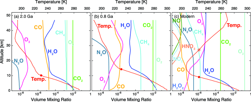
Figure 1: Vertical profiles of temperature (red dashed line) and gaseous species (solid lines) for three different Earth-like trajectory epochs, 2.0 Ga (a), 0.8 Ga (b), and the modern Earth (c). Red circles represent the 230 K threshold altitude of water and ice clouds, which are 10.3, 14.4, and 8.71 km for the cases of 2.0 Ga, 0.8 Ga, and the modern Earth, respectively. Note that most abundant species $\mathrm{N_{2}}$ is not shown.

Table 1: Geological constraints on the past $\mathrm{O_{2}}$ abundances

Epoch [Ga.]	Concentration	Reference
2.45-0.42	0.01-0.4 PAL	Kump (2008) and references therein
2.1-0.8	$10^{-4}-0.1$ PAL	Lyons et al. (2014) and references therein
1.8-0.8	$<0.001$ PAL	Planavsky et al. (2014)
0.42-	0.6-1.6 PAL	Kump (2008) and references therein

Note. — PAL stands for the present atmospheric level.

As for clouds, we assume water (cumulus) clouds for temperature above 230 K and ice (cirrus) clouds for that below 230 K following Zsom et al. (2012). We insert continuum-absorbing/emitting layers similar to some previous works (Des Marais et al., 2002; Kaltenegger et al., 2007; Rugheimer et al., 2013, 2015a; Rugheimer & Kaltenegger, 2018). While planets with a surface ocean, an active hydrological cycle, and abundant water vapor have abundant clouds, dry habitable planets, which have been proposed to extend the habitable zone inward (e.g., Abe et al., 2005, 2011; Zsom et al., 2013; Kodama et al., 2015), have fewer clouds (e.g., Kodama et al., 2018). However, since the cloud properties in exoplanet contains large uncertainty, we simply vary the altitude of the cloud layer and its coverage systematically to explore the effect of these cloud properties on reflectance spectra of Earth-like exoplanets.

We assume surface compositions following Rugheimer & Kaltenegger (2018): The surface consists of 70% ocean, 2% coast, and 28% land for all the epochs considered. For 2.0 Ga and 0.8 Ga cases, the land is composed of 35% basalt, 40% granite, 15% snow, and 10% sand, while 30% grass, 30% trees, 9% granite, 9% basalt, 15% snow, and 7% sand for modern case. We take reflectivity data for clouds and surface compositions from the ASTER Spectral Library (Baldridge et al., 2009) and the USGS Spectral Library (Kokaly et al., 2017). We adopt the average planet phase angle of $\frac{\pi}{2}$ (i.e., quadrature). For the input stellar spectra of the Sun at each epoch, we use a solar evolution model (Claire et al., 2012).

2.2 LUVOIR Coronagraph Noise Simulator

We calculate the impact of noise on the detection of spectral features considering the Earth-like planet located at 5 pc away from the Earth. For this purpose, we use the instrument noise model from Robinson et al. (2016) originally developed for WFIRST-AFTA. We have modified this noise calculator to match the potential LUVOIR values. While two plans have been proposed for the telescope diameter of LUVOIR, 15 m and 8 m, in this study, we use the value of 10 m as an example. Considering visible channel of ECLIPS instrument, we take its value for the instrument spectral resolution and coronagraph inner and outer working angle from Table 9.2 of the LUVOIR interim report. All the input values we use are listed in Table 2. Also, while the original noise model assumed the black-body for the stellar spectrum, we use a solar spectrum evolution model as the input.

Following Robinson et al. (2016), we explore the integration time required to detect a molecular feature by defining it as the time to achieve $\mathrm{S/N}=5$. We define the signal as the difference between the spectra calculated with and without the specific molecular absorption, while Robinson et al. (2016) defined it as the deviation from a flat continuum; we substitute the photon count rate for the case of the spectrum calculated without considering the absorption of a certain molecule for the continuum count rate in Eq. (7) of Robinson et al. (2016). The model selects a wavelength element within a specific wavelength range from a given instrument spectral resolution. We will mention the wavelength range we adopt for each molecular absorption feature in §4. Note that in order to recover molecular abundances, a measurement of the flux at the bottom of the absorption features is important.

Table 2: Values of parameters used in this study

Description	Value	Reference
Distance to observed star-planet system	5 pc
Planetary radius	1 $R_{\earth}$
Planet-star distance	1 AU
Planet phase angle	$90^{\circ}$
Number of exodis in exoplanetary disk	1
Coronagraph design contrast	$10^{-10}$
Telescope diameter	10 m
Instrument spectral resolution	140	LUVOIR interim report
Telescope and instrument throughput	0.20
Coronagraph inner working angle [$\lambda/D$]	3.5	LUVOIR interim report
Coronagraph outer working Angle [$\lambda/D$]	64.0	LUVOIR interim report
Width of photometric aperture [$\lambda/D$]	1.5

3 Results: Influence of clouds on spectra of Earth-like planets

In this section, we systematically explore the effect of cloud properties, namely the altitude of the cloud layer (§3.1) and its coverage (§3.2) on reflectance spectra of an Earth-like planet. Then in §3.3, we compare the spectrum models of the Earth-like planets at different geological epochs, focusing on the $\mathrm{O_{2}}$ A-band feature since $\mathrm{O_{2}}$ has long been considered as a key target molecule for future missions.

3.1 Altitude of Cloud Layer

Figure 2 shows spectral models for an atmosphere with 100% cloud coverage at three different altitudes, 17 km (blue line), 9.5 km (green line), and 2.2 km (red line). Water clouds are assumed for 2.2 km case, while ice clouds for 17 and 9.5 km cases. A clear sky atmosphere is also plotted (black) for reference. One finds that in the spectrum of a clear sky atmosphere, most of the molecular absorption features come from $\mathrm{H_{2}O}$, which are located at 0.71-0.74, 0.80-0.84, 0.90-0.98, 1.1-1.2, 1.3-1.5, and 1.8-2.0 $\mu$m, while the distinct $\mathrm{O_{2}}$ A-band feature exists at 0.76 $\mu$m along with smaller $\mathrm{O_{2}}$ B-band feature at 0.69 $\mu$m.

Clouds increase the flux because of their high albedo. At relatively short wavelengths ($\lesssim 0.9$ $\mu$m), where the atmosphere is relatively optically thick and the optical properties of water and ice clouds are almost similar, the lower the altitude of the cloud layer is, the larger the overall (continuum) flux becomes. This behavior is due to the increased Rayleigh scattering of molecules above the cloud layer in the lower atmosphere. For the lower altitude clouds, the absorption feature is deeper, and the flux is lower in the core of the line. This is because there is a larger column-integrated concentration of the species above the cloud layer (see also Tinetti et al., 2006a, b; Kitzmann et al., 2011).

In contrast, at relatively long wavelengths ($\gtrsim 0.9$ $\mu$m), where the atmosphere is optically thinner, the features are created mostly by clouds, while the molecular absorption also contribute for the lower altitude cloud case of 2.2 km. Note that water clouds have absorption at the similar wavelength region as gaseous water. For the higher altitude ice cloud cases of 17 and 9.5 km, due to the negligible column-integrated concentration of the species above the cloud layer for the both cases, the spectra are similar and completely characterized by less reflective optical properties of ice clouds.

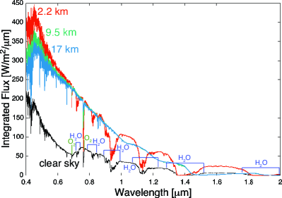
Figure 2: Reflective Spectra for a modern Earth-like atmosphere with 100% cloud coverage at three different altitudes, 17 km (blue line), 9.5 km (green line), and 2.2 km (red line). Water clouds are assumed for 2.2 km case, while ice clouds for 17 and 9.5 km cases. A clear sky atmosphere is plotted in black line for reference. Note that the spectral models are smoothed for clarity by averaging over the wavenumber range of $20.1~{}\mathrm{cm}^{-1}$ at each outputted wavenumber point with a grid of $0.1~{}\mathrm{cm}^{-1}$. We use the same smoothing method for the results of spectrum models hereafter.

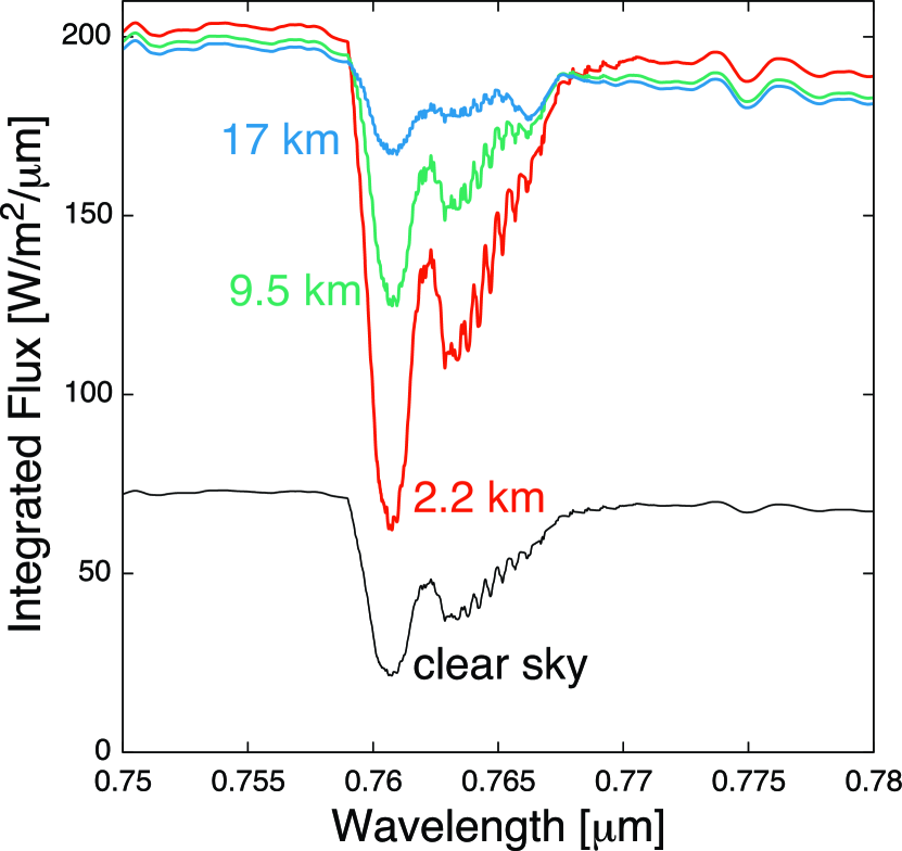
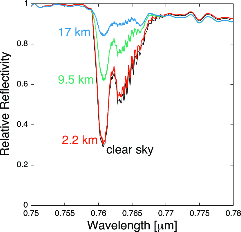
Figure 3: Same as Fig. 2 with only the $\mathrm{O_{2}}$ A-band feature shown in integrated flux (left) and relative reflectivity (right). The relative reflectivity is calculated by normalizing with the maximum flux between the wavelength range of 0.75-0.78 $\mu$m.

The left panel of Figure 3 is the zoomed in view of Fig. 2 around the $\mathrm{O_{2}}$ A-band feature. Note that the difference of the reflectivity of water and ice clouds is little in this wavelength region. The flux at the peak of the absorption feature is smaller for the lower cloud layer, while that at the continuum is larger as noted above. We show relative reflectivity in the right panel of Figure 3 calculated by normalizing the flux with the maximum flux between the wavelength range of 0.75-0.78 $\mu$m. For the lower altitude clouds, the relative reflectivity of the feature becomes deeper due to the larger absorption at the core of the feature and increased Rayleigh scattering at the continuum.

3.2 Cloud Coverage

Next, we examine the dependence of the fractional cloud coverage on the spectra. The top left panel (a) of Figure 4 shows the Earth-like spectra with ice cloud layers of 17 km altitude, while the top right one (b) shows those with 2.2 km water cloud layers, for 0% (black), 50% (blue), and 100% (red) cloud coverage. Again, the difference of the reflectivity of water and ice clouds is little in this wavelength region. For the 17 km cloud case (a), the flux at the depth of the absorption feature varies more with cloud coverage than compared to the 2.2 km case (b) because the flux at the core of the feature is determined by the amount of the absorption, namely column-integrated O₂ concentration of the species above the cloud layer. The continuum increases with increasing cloud coverage due to the higher albedo of water clouds compared to the surface reflectivity.

The bottom two panels of Fig. 4 (c, d) are the same as the top two panels of Fig. 4 (a, b), but with relative reflectivity. It can be seen that for the 17 km case (c), the relative absorption varies greatly with the cloud coverage and is deeper for the lower cloud coverage due to blocking more of the atmosphere below the cloud layer. While for the 2.2 km case (d), the relative reflectivity hardly varies with the cloud coverage although it is slightly shallower for the higher cloud coverage.

Our results for the modern Earth case confirm previous findings by Tinetti et al. (2006a, b); Kaltenegger et al. (2007); Kitzmann et al. (2011). We will now consider the case of earlier geological epochs in §3.3 and calculate the detectability of these features with a LUVOIR sized telescope in §4.

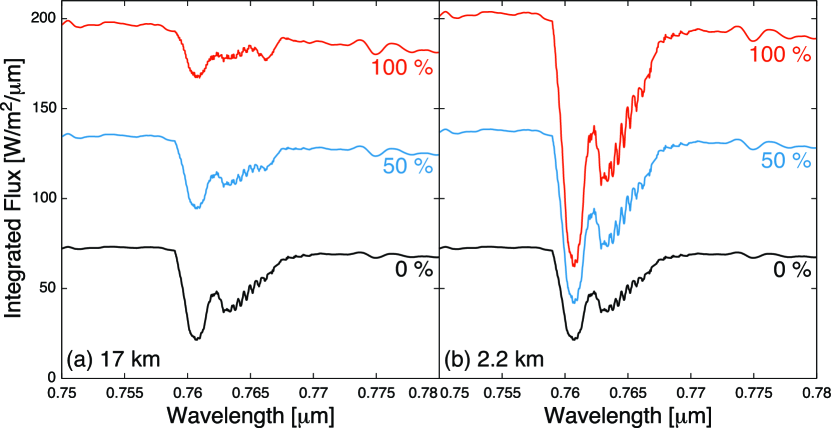
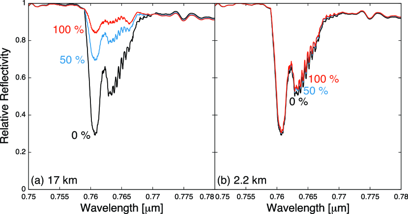
Figure 4: The $\mathrm{O_{2}}$ A-band with ice cloud layers of 17 km (left two panels) and 2.2 km altitude water cloud layers (right two panels) with 0% (black), 50% (blue), and 100% (red) cloud coverage plotted with integrated flux (top two panels) and relative absorption (bottom two panels).

3.3 Evolution of the Planet

In this section, we explore the spectra of an Earth-like planet at different levels of oxygen and geological epochs. The abundance of $\mathrm{O_{2}}$ in the Earth’s atmosphere has varied over time but broadly rose after two oxygenation events known as the Great Oxygenation Event (GOE) and the Neoproterozoic Oxygenation Event (NOE) (Lyons et al., 2014). We adopt concentrations of 0.01 PAL, 0.1 PAL, and 1.0 PAL for 2.0 Ga, 0.8 Ga, and the present, respectively, where PAL stands for the present atmospheric level. Note that oxygen levels during the Proterozoic are debated and estimates range from $<0.001$ PAL to 0.4 PAL (Canfield, 2005; Kump, 2008; Planavsky et al., 2014) as listed in Table 1. To explore the effect of $\mathrm{O_{2}}$ abundance on the spectra in detail, we also consider the case of 0.5 PAL $\mathrm{O_{2}}$ as a middle value. We calculate the spectrum model of the 0.5 PAL case using the same inputs to the radiative transfer model as modern Earth except for $\mathrm{O_{2}}$ abundance. Note this treatment is valid as long as one compares the spectrum models only around the wavelength range of $\mathrm{O_{2}}$ absorption features.

Figure 5 shows the spectrum for four different $\mathrm{O_{2}}$ abundance models, 0.01 PAL (2.0 Ga, purple), 0.1 PAL (0.8 Ga, light blue), 0.5 PAL (green), and 1.0 PAL (0.0 Ga, orange) assuming 60% cloud coverage with a 2.2 km water cloud layer. As expected, the absorption feature is deeper for larger $\mathrm{O_{2}}$ abundance.

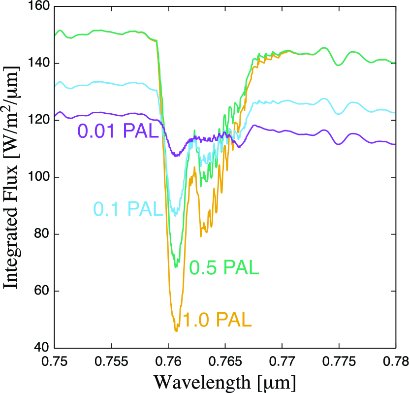
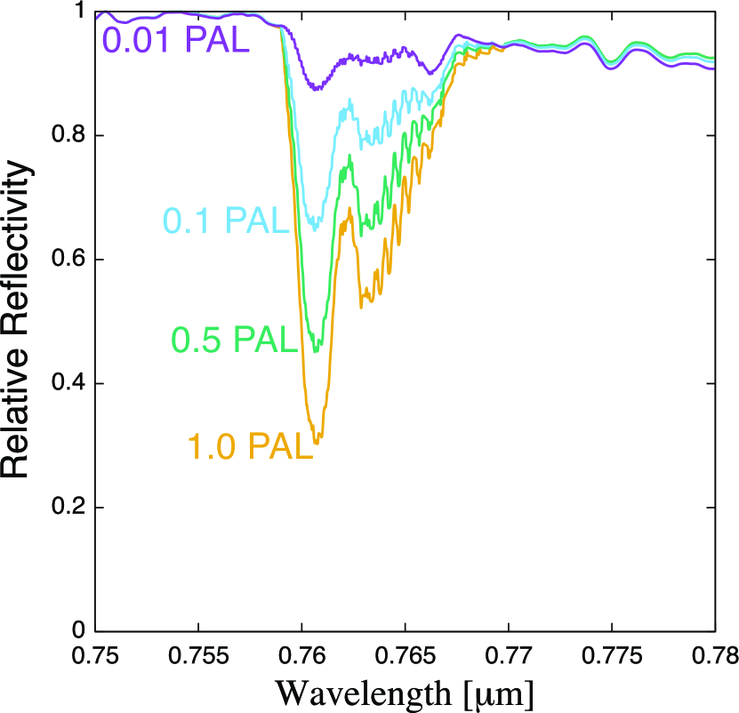
Figure 5: Integrated Flux (left) and relative reflectivity (right) spectral models for four different $\mathrm{O_{2}}$ abundances, 0.01 PAL (2.0 Ga, purple), 0.1 PAL (0.8 Ga, light blue), 0.5 PAL (green), and 1.0 PAL (modern, orange) assuming a 2.2 km water cloud layer altitude with 60% cloud coverage.

4 Results: Detectability of $\mathrm{O_{2}}$, $\mathrm{H_{2}O}$, and $\mathrm{CH_{4}}$ with LUVOIR

In this section, we explore the detectability of the features of astrobiologically important gaseous molecules in the visible and near-infrared region of the Earth-like spectrum, namely $\mathrm{O_{2}}$, $\mathrm{H_{2}O}$, and $\mathrm{CH_{4}}$ with proposed space telescope LUVOIR.

Figure 6 shows the modern Earth-like spectra of a clear sky atmosphere (black) and the same atmosphere with a 100% water cloud coverage layer at 2.2 km (red) along with 1$\sigma$ observational errors for 10-hour observation with a LUVOIR-sized telescope calculated with the noise model. The assumed distance to the planetary system is 5 pc. Note the negative flux means that the measurement is consistent with zero flux since a Sun-like star has low flux in the NIR.

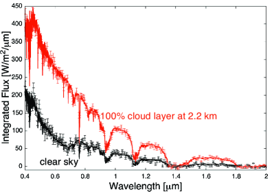
Figure 6: Modern Earth-like spectra of a clear sky atmosphere (black) and the same atmosphere with a 100% water cloud coverage layer at 2.2 km (red) along with 1$\sigma$ observational errors for 10-hour observation with a LUVOIR-sized telescope calculated with the noise model. The assumed distance to the planetary system is 5 pc.

4.1 $\mathrm{O_{2}}$ Feature

Figure 7 shows spectrum models for the Earth-like atmosphere with 60% cloud coverage at different altitudes, 17 km (blue), 9.5 km (green), and 2.2 km (red) around the $\mathrm{O_{2}}$ A-band feature with 1$\sigma$ observational errors for 10-hour observation calculated with the noise model for four different $\mathrm{O_{2}}$ abundances, 0.01 PAL (a), 0.1 PAL (b), 0.5 PAL (c), 1.0 PAL (d). Water clouds are assumed for the cases of 9.5 and 2.2 km cloud layers of 0.01 and 0.1 PAL $\mathrm{O_{2}}$ abundances and 2.2 km cloud layers of 0.5 and 1.0 PAL $\mathrm{O_{2}}$ abundances, while ice clouds are assumed for the other cases. The assumed distance to the planetary system is 5 pc.

Again, note that the difference of the reflectivity of water and ice clouds in this wavelength region is minimal. We also note that we present the results on the grids we run the simulations and the stark contour lines come from our low-resolution grids.

We find that the observational 1$\sigma$ error bars are much larger than the $\mathrm{O_{2}}$ absorption feature depth for the 0.01 PAL $\mathrm{O_{2}}$ concentration case (a), but comparable or smaller for larger $\mathrm{O_{2}}$ concentration cases of 0.1 PAL (b), 0.5 PAL (c), and 1.0 PAL (d), especially for the cases of cloud layers at the lower altitudes. The integration time required to detect the $\mathrm{O_{2}}$ A-band feature with the proposed LUVOIR telescope with $\mathrm{S/N}=5$ for the 2.2 km altitude cloud layer and 0.5 PAL $\mathrm{O_{2}}$ concentration case (red line in Fig. 7c) is 9.4 hour, almost the same as the assumed observation time. Here, we assume the wavelength region of the feature is 0.759-0.769 $\mathrm{\mu}$m. The detection time for each case in Fig. 7 is tabulated in Table 3.

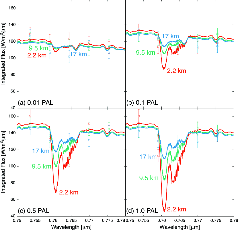
Figure 7: $\mathrm{O_{2}}$ A-band feature for the Earth-like atmosphere with 60% cloud coverage at different altitudes, 17 km (blue), 9.5 km (green), and 2.2 km (red) with 1$\sigma$ observational errors for 10-hour observation calculated with the noise model for four different $\mathrm{O_{2}}$ abundances, 0.01 PAL (a), 0.1 PAL (b), 0.5 PAL (c), 1.0 PAL (d). Water clouds are assumed for the cases of 9.5 and 2.2 km cloud layers of 0.01 and 0.1 PAL $\mathrm{O_{2}}$ abundances and 2.2 km cloud layers of 0.5 and 1.0 PAL $\mathrm{O_{2}}$ abundances, while ice clouds are assumed for the other cases.

Table 3: Integration time [hour] required to detect $\mathrm{O_{2}}$ A-band feature of 0.759-0.769 $\mathrm{\mu}$m in the atmosphere of Earth-like planet located at 5 pc away with the proposed LUVOIR telescope with $\mathrm{S/N}=5$ for the cases of three different cloud layer altitudes, 17, 9.5, and 2.2 km and four different $\mathrm{O_{2}}$ abundances, 0.01, 0.1, 0.5, 1.0 PAL. The assumed cloud coverage is 60%.

	Altitude of cloud layer
$\mathrm{O_{2}}$ abundance	17 km	9.5 km	2.2 km
0.01 PAL	4800	1800	470
0.1 PAL	380	130	33
0.5 PAL	85	30	9.4
1.0 PAL	47	16	5.2

Figure 8 shows an intensity plot for the integration time required to detect the $\mathrm{O_{2}}$ A-band feature with $\mathrm{S/N}=5$ for four different $\mathrm{O_{2}}$ abundances, 0.01 PAL (a), 0.1 PAL (b), 0.5 PAL (c), and 1.0 PAL (d) with varying cloud altitude and coverage. The assumed wavelength region for the feature is 0.759-0.769 $\mathrm{\mu}$m. For high altitude ($\gtrsim 10$ km for the modern case) clouds, a lower cloud coverage makes the feature deeper and the detection easier despite the smaller continuum flux for a lower cloud coverage (see Fig. 4a,c). For low altitude ($\lesssim 10$ km for the modern case) clouds, a higher cloud coverage increases the flux at the continuum, while almost the same relative depth of the feature regardless of the cloud coverage, and thus makes the detection easier for a higher cloud coverage (see Fig. 4b, d).

As seen in Fig. 8, for the proposed LUVOIR telescope the integration time needed to detect the $\mathrm{O_{2}}$ A-band feature for an Earth-like atmosphere with $\mathrm{O_{2}}$ abundance of 0.01 PAL (a) will take typically more than 1000 hours for the majority of the cloud parameters. The best case scenario would be for a widespread low layer cloud, which would then make the feature detectable with 100 hours. For 0.1 PAL, 0.5 PAL, and 1.0 PAL O₂ cases, for the majority of the cloud parameter space the detection will take approximately 100, 30, and 10 hours, respectively (see Fig 8). For the cloud parameter end cases, the minimum and maximum detection times are 10 to 600 hours for the 0.1 PAL case, 3 to 300 hours for the 0.5 PAL case, and 2 to 200 hours for the 1 PAL O₂ case. Especially, for the atmospheres with 0.5 and 1.0 PAL $\mathrm{O_{2}}$ abundances, the feature will be detectable with integration time $\lesssim 10$ hours as long as there are lower altitude ($\lesssim 8$ km) clouds with a global coverage of $\gtrsim 20\%$. Note that modern Earth has a global cloud coverage of $\sim$50-60% (Tinetti et al., 2006a; Robinson et al., 2011).

Figure 8: Intensity plots for the integration time required to detect the $\mathrm{O_{2}}$ A-band feature of 0.759-0.769 $\mathrm{\mu}$m with $\mathrm{S/N}=5$ are shown for four different $\mathrm{O_{2}}$ abundances, 0.01 PAL (2.0 Ga) (a), 0.1 PAL (0.8 Ga) (b), 0.5 PAL (c), and 1.0 PAL (modern) (d) with varying cloud altitude and coverage. Contour lines for the integration time are also plotted in black solid and dashed lines. Also, the black filled circles on the vertical axes represent the altitude at 230 K, above which clouds are assumed as ice ones.

4.2 $\mathrm{H_{2}O}$ Feature

Among the several $\mathrm{H_{2}O}$ features at 0.71-0.74, 0.80-0.84, 0.90-0.98, 1.1-1.2, 1.3-1.5, and 1.7-2.0 $\mu$m, we explore the detectability of the strongest feature at 0.90-0.98 $\mathrm{\mu}$m in this section. Figure 9 shows an intensity plot for the integration time required to detect the $\mathrm{H_{2}O}$ feature of 0.900-0.980 $\mathrm{\mu}$m with $\mathrm{S/N}=5$ for three different Earth-trajectory epochs, 2.0 Ga (a), 0.8 Ga (b), and modern Earth (c) with varying cloud altitude and coverage. Same as the $\mathrm{O_{2}}$ case, for high altitude ($\gtrsim 3$ km for the modern case) clouds, a lower cloud coverage makes the feature deeper and the detection easier, while for low altitude ($\lesssim 3$ km for the modern case) clouds, a high cloud coverage makes the detection easier due to the increased flux at the continuum. While the water clouds also have absorption at this wavelength, the ice clouds do not have such absorption and thus their relatively reflective properties basically make the required integration time slightly smaller.

Compared to the $\mathrm{O_{2}}$ case (§4.1), the detection time for the $\mathrm{H_{2}O}$ feature significantly depends on the cloud properties, namely altitude and coverage. Except for the extreme case of higher coverage ($\gtrsim 80$% for the modern case) clouds at high altitudes ($\gtrsim 6$ km for the modern case), for all the three epochs, the detection of the $\mathrm{H_{2}O}$ feature will take approximately 3-10 hours, an order of magnitude smaller than that for the $\mathrm{O_{2}}$ feature. For the extreme cases, the minimum and maximum detection times are 0.4 to $6\times 10^{4}$ hours for the 2.0 Ga case, 0.2 to $9\times 10^{3}$ hours for the 0.8 Ga case, and 0.4 to $3\times 10^{5}$ hours for the modern case (see Fig. 9). The very large detection times for the high altitude and high cloud coverage case is due to H₂O being less abundant in the upper atmosphere for planets with a cold trap, whereas O₂ is well mixed.

Note the water abundance for the two earlier geological epochs in our models is largely determined by increased evaporation due to higher surface temperatures from a larger greenhouse effect despite a lower solar luminosity.

Figure 9: Intensity plots for the integration time required to detect the $\mathrm{H_{2}O}$ feature of 0.90-0.98 $\mathrm{\mu}$m with $\mathrm{S/N}=5$ are shown for three different Earth-like trajectory epochs, 2.0 Ga (a), 0.8 Ga (b), and the modern Earth (c) with varying cloud altitude and coverage. Contour lines for the integration time are also plotted in black solid and dashed lines. Note that the black dashed lines are for the integration times of 0.3, 3, 30, 300, $3\times 10^{3}$, $3\times 10^{4}$, and $3\times 10^{5}$ hr but not labeled for the clarity. Also, the black filled circles on the vertical axes represent the altitude at 230 K, above which clouds are assumed as ice ones.

4.3 $\mathrm{CH_{4}}$ Feature

Figure 10 shows an intensity plot for the integration time required to detect the strongest reflected light NIR $\mathrm{CH_{4}}$ feature at 1.64-1.78 $\mathrm{\mu}$m with $\mathrm{S/N}=5$ for three different Earth-trajectory epochs, 2.0 Ga (a), 0.8 Ga (b), and modern Earth (c) with varying cloud altitude and coverage.

Contrary to the cases of $\mathrm{O_{2}}$ and $\mathrm{H_{2}O}$, the optical properties of water and ice clouds are quite different in this wavelength region with much higher reflectivity for water clouds, and this causes the changes of the trend at the threshold altitudes. For the water cloud region at the lower altitudes, the lower the altitude of the cloud layer becomes, and the higher the cloud coverage becomes, the detection time becomes smaller. This is because of the larger column-integrated concentration of the species above the cloud layer and the relatively reflective properties of water clouds compared to the surface. However, in the ice cloud region at the higher altitudes, the lower the altitude of the cloud layer becomes, and the lower the cloud coverage becomes, the detection time becomes smaller. This is due to the larger column-integrated concentration of the species above the cloud layer and the relatively absorbing properties of ice clouds compared to the surface in this wavelength range.

The detection of the $\mathrm{CH_{4}}$ feature will take approximately 10 and 30 hours for 2.0 Ga and 0.8 Ga cases, respectively. For the extreme cloud parameter cases, the minimum and maximum detection times are 1 to 300 hours for the 2.0 Ga case and 2 to 900 hours for the 0.8 Ga case. Here we note that the $\mathrm{CH_{4}}$ abundances for 2.0 Ga and 0.8 Ga cases are not well-constrained and the values we adopt may be optimistic (e.g., Reinhard et al., 2017).

For the modern Earth case, however, it will take more than 6000 hours for all the cloud parameters modeled and the feature is undetectable even with the LUVOIR-sized telescope regardless of the cloud parameters because of the relatively low $\mathrm{CH_{4}}$ abundance in the modern atmosphere and the weaker NIR feature as compared with the IR CH₄ feature. For the extreme cases, the minimum and maximum detection times are 6000 to $3\times 10^{7}$ hours for the modern case (see Fig. 10). The trend for the modern Earth case is the same as the 2.0 Ga and 0.8 Ga cases.

Figure 10: Intensity plots for the integration time required to detect the $\mathrm{CH_{4}}$ feature of 1.64-1.78 $\mathrm{\mu}$m with $\mathrm{S/N}=5$ are shown for three different Earth-like trajectory epochs, 2.0 Ga (a), 0.8 Ga (b), and the modern Earth (c) with varying cloud altitude and coverage. Contour lines for the integration time are also plotted in black solid and dashed lines. Also, the black filled circles on the vertical axes represent the altitude at 230 K, above which clouds are assumed as ice ones.

5 Discussion

In this study, we have examined the impact of cloud properties (cloud altitude and its coverage) on the detectability of the molecules on the reflectance spectra of an Earth-like planet at different geological epochs systematically. A self-consistent microphysical model (e.g., Zsom et al., 2012; Ohno & Okuzumi, 2017, 2018; Powell et al., 2018; Gao & Benneke, 2018; Ormel & Min, 2019) would be needed to examine the plausibility of these cloud parameters, which is beyond the scope of this study. In our two-stream radiative transfer model, the cloud layer is assumed to be completely absorbing or reflective surface. In reality, however, some light can penetrate the cloud layer depending on the thickness of the cloud layer, and the cloud particle size. This effect also cannot be studied without deriving the distributions of the size and number density of the cloud particles by a microphysical cloud model and by using a multi-scattering radiative transfer model.

For all the cases of detecting the $\mathrm{O_{2}}$ A-band, $\mathrm{H_{2}O}$ feature at 0.90-0.98 $\mathrm{\mu}$m, and that of $\mathrm{CH_{4}}$ at 1.64-1.78 $\mathrm{\mu}$m, we have found that the shortest integration times are for a high-coverage, low-altitude cloud layer due to the deeper absorption created with increased back-scattered light of the higher albedo cloud layer when compared with the surface albedo and the larger integrated column density. It is possible that this same effect on the detectability could be seen on a snowball planet (e.g., Tajika, 2008; Kadoya & Tajika, 2014, 2015, 2016). While the colder temperatures may slow down bioproductivity, Earth has been through several snowball states with global glaciation well after oxygen has been a major atmospheric constituent and even quite recent in its history (see Kirschvink, 1992; Hoffman et al., 2017, and references therein). These snowball states may make these features easier to detect as long as there are appreciable levels of these species in the atmosphere. As for the abundance of $\mathrm{H_{2}O}$, although we have assumed larger abundances for the two earlier geological epochs, during the cooler period within the huge temporal range of temperature oscillation, it might be lower than what we have assumed, making the detection more difficult.

While we explored the detectability of specific absorption features of $\mathrm{O_{2}}$, $\mathrm{H_{2}O}$, and $\mathrm{CH_{4}}$ via the low-resolution measurement of the flux-contrast around the wavelength range of absorption features by LUVOIR, Wang et al. (2018) investigated the detection time of $\mathrm{O_{2}}$, $\mathrm{H_{2}O}$, $\mathrm{CH_{4}}$, and $\mathrm{CO_{2}}$ via high-resolution cross-correlation technique over the wavelength range of $0.5-1.8$ $\mu$m by HabEx and LUVOIR. In their LUVOIR case, considering an modern Earth-like planet with a clear sky atmosphere located at 5 pc away, they reported that the required starlight suppression for an exposure time of 100 hours are $\sim 2\times 10^{-9}$ and $\sim 10^{-8}$ for $\mathrm{H_{2}O}$ and $\mathrm{O_{2}}$, respectively, while $\mathrm{CH_{4}}$ and $\mathrm{CO_{2}}$ are undetectable with 100-hour exposure time.

6 Summary

In this study, we have explored the effect of cloud altitude and its coverage on the reflectance spectra of Earth-like planets at different geological epochs and examined the detectability of astrobiologically interesting gaseous molecules in the visible and near-infrared spectrum, namely $\mathrm{O_{2}}$, $\mathrm{H_{2}O}$, and $\mathrm{CH_{4}}$, by simulating instrumental noise for the proposed mission concept LUVOIR.

Considering an Earth-like planet located at 5 pc away, we have found that for the proposed LUVOIR telescope, the detection of the $\mathrm{O_{2}}$ A-band feature (0.76 $\mathrm{\mu}$m) will take approximately 100, 30, and 10 hours for the majority of the cloud parameters modeled for atmospheres with 0.1, 0.5, and 1.0 PAL O₂ abundances, respectively. Especially, for 0.5 and 1.0 PAL $\mathrm{O_{2}}$ cases, the feature could be detectable with integration times $\lesssim 10$ hours as long as there are lower altitude ($\lesssim 8$ km) clouds with a global coverage of $\gtrsim 20\%$. For 0.01 PAL O₂ case, however, it will take more than 100 hours for all the cloud parameters modeled.

The combined detection of O₂ and CH₄ remains the strongest biosignature. There is currently no known abiotic oxygen production mechanism which would persist with a simultaneously dedectable amount of CH₄ present. For $\mathrm{CH_{4}}$, we have found that the detection of its NIR feature at 1.64-1.78 $\mathrm{\mu}$m will take approximately 10 and 30 hours for 2.0 Ga and 0.8 Ga cases, respectively.

For the modern Earth case, however, it will take more than 6000 hours for all the cloud parameters modeled and the feature is undetectable even with the LUVOIR-sized telescope because of the relatively low $\mathrm{CH_{4}}$ abundance in the modern atmosphere.

While H₂O is not a biosignature, it is an important indicator of habitability and provides necessary context for interpreting future exoplanet observations. For $\mathrm{H_{2}O}$ feature at 0.90-0.98 $\mathrm{\mu}$m, we have found that except for the extreme case of higher cloud coverage at high altitudes, the detection of its strongest feature will take approximately 3-10 hours.

In summary, a LUVOIR-sized mission with a coronagraph could detect the reflected light of O₂, CH₄, and H₂O for many cases comparable to Earth’s geological history with a wide range of cloud parameters. To detect the combination of these gases with less than 100 hours of observation time, however, will require more CH₄ than in modern Earth’s atmosphere, O₂ levels around 0.1 PAL or greater, and clouds that are lower in altitude or patchy in coverage.

References

- Abe et al. (2011) Abe, Y., Abe-Ouchi, A., Sleep, N. H., & Zahnle, K. J. 2011, Astrobiology, 11, 443, doi: 10.1089/ast.2010.0545
- Abe et al. (2005) Abe, Y., Numaguti, A., Komatsu, G., & Kobayashi, Y. 2005, Icarus, 178, 27, doi: 10.1016/j.icarus.2005.03.009
- Anglada-Escudé et al. (2016) Anglada-Escudé, G., Amado, P. J., Barnes, J., et al. 2016, Nature, 536, 437, doi: 10.1038/nature19106
- Baldridge et al. (2009) Baldridge, A., Hook, S., Grove, C., & Rivera, G. 2009, Remote Sensing of Environment, 113, 711 , doi: https://doi.org/10.1016/j.rse.2008.11.007
- Canfield (2005) Canfield, D. E. 2005, Annual Review of Earth and Planetary Sciences, 33, 1, doi: 10.1146/annurev.earth.33.092203.122711
- Claire et al. (2006) Claire, M. W., Catling, D. C., & Zahnle, K. J. 2006, Geobiology, 4, 239
- Claire et al. (2012) Claire, M. W., Sheets, J., Cohen, M., et al. 2012, ApJ, 757, 95, doi: 10.1088/0004-637X/757/1/95
- Des Marais et al. (2002) Des Marais, D. J., Harwit, M. O., Jucks, K. W., et al. 2002, Astrobiology, 2, 153, doi: 10.1089/15311070260192246
- Dittmann et al. (2017) Dittmann, J. A., Irwin, J. M., Charbonneau, D., et al. 2017, Nature, 544, 333, doi: 10.1038/nature22055
- Domagal-Goldman et al. (2014) Domagal-Goldman, S. D., Segura, A., Claire, M. W., Robinson, T. D., & Meadows, V. S. 2014, ApJ, 792, 90, doi: 10.1088/0004-637X/792/2/90
- Feng et al. (2018) Feng, Y. K., Robinson, T. D., Fortney, J. J., et al. 2018, AJ, 155, 200, doi: 10.3847/1538-3881/aab95c
- Gao & Benneke (2018) Gao, P., & Benneke, B. 2018, ApJ, 863, 165, doi: 10.3847/1538-4357/aad461
- Gao et al. (2015) Gao, P., Hu, R., Robinson, T. D., Li, C., & Yung, Y. L. 2015, ApJ, 806, 249, doi: 10.1088/0004-637X/806/2/249
- Gillon et al. (2017) Gillon, M., Triaud, A. H. M. J., Demory, B.-O., et al. 2017, Nature, 542, 456, doi: 10.1038/nature21360
- Haqq-Misra et al. (2008) Haqq-Misra, J. D., Domagal-Goldman, S. D., Kasting, P. J., & Kasting, J. F. 2008, Astrobiology, 8, 1127, doi: 10.1089/ast.2007.0197
- Harman et al. (2015) Harman, C. E., Schwieterman, E. W., Schottelkotte, J. C., & Kasting, J. F. 2015, ApJ, 812, 137, doi: 10.1088/0004-637X/812/2/137
- Hoffman et al. (2017) Hoffman, P. F., Abbot, D. S., Ashkenazy, Y., et al. 2017, Science Advances, 3, e1600983
- Hu et al. (2012) Hu, R., Seager, S., & Bains, W. 2012, ApJ, 761, 166, doi: 10.1088/0004-637X/761/2/166
- Kadoya & Tajika (2014) Kadoya, S., & Tajika, E. 2014, ApJ, 790, 107, doi: 10.1088/0004-637X/790/2/107
- Kadoya & Tajika (2015) —. 2015, ApJ, 815, L7, doi: 10.1088/2041-8205/815/1/L7
- Kadoya & Tajika (2016) —. 2016, ApJ, 825, L21, doi: 10.3847/2041-8205/825/2/L21
- Kaltenegger & Traub (2009) Kaltenegger, L., & Traub, W. A. 2009, ApJ, 698, 519, doi: 10.1088/0004-637X/698/1/519
- Kaltenegger et al. (2007) Kaltenegger, L., Traub, W. A., & Jucks, K. W. 2007, ApJ, 658, 598, doi: 10.1086/510996
- Kasting & Ackerman (1986) Kasting, J. F., & Ackerman, T. P. 1986, Science, 234, 1383, doi: 10.1126/science.234.4782.1383
- Kawashima et al. (2019) Kawashima, Y., Hu, R., & Ikoma, M. 2019, arXiv e-prints. https://arxiv.org/abs/1902.10151
- Kawashima & Ikoma (2018) Kawashima, Y., & Ikoma, M. 2018, ApJ, 853, 7, doi: 10.3847/1538-4357/aaa0c5
- Kawashima & Ikoma (2019) —. 2019, ApJ, submitted
- Kirschvink (1992) Kirschvink, J. L. 1992
- Kitzmann et al. (2013) Kitzmann, D., Patzer, A. B. C., & Rauer, H. 2013, A&A, 557, A6, doi: 10.1051/0004-6361/201220025
- Kitzmann et al. (2011) Kitzmann, D., Patzer, A. B. C., von Paris, P., Godolt, M., & Rauer, H. 2011, A&A, 534, A63, doi: 10.1051/0004-6361/201117375
- Kodama et al. (2015) Kodama, T., Genda, H., Abe, Y., & Zahnle, K. J. 2015, ApJ, 812, 165, doi: 10.1088/0004-637X/812/2/165
- Kodama et al. (2018) Kodama, T., Nitta, A., Genda, H., et al. 2018, Journal of Geophysical Research (Planets), 123, 559, doi: 10.1002/2017JE005383
- Kokaly et al. (2017) Kokaly, R. F., Clark, R. N., Swayze, G. A., et al. 2017, USGS spectral library version 7, Tech. rep., US Geological Survey
- Kreidberg et al. (2014) Kreidberg, L., Bean, J. L., Désert, J.-M., et al. 2014, Nature, 505, 69, doi: 10.1038/nature12888
- Kump (2008) Kump, L. R. 2008, Nature, 451, 277
- Lederberg (1965) Lederberg, J. 1965, Nature, 207, 9, doi: 10.1038/207009a0
- Lovelock (1965) Lovelock, J. E. 1965, Nature, 207, 568, doi: 10.1038/207568a0
- Luger & Barnes (2015) Luger, R., & Barnes, R. 2015, Astrobiology, 15, 119, doi: 10.1089/ast.2014.1231
- Luo et al. (2016) Luo, G., Ono, S., Beukes, N. J., et al. 2016, Science Advances, 2, e1600134
- Lyons et al. (2014) Lyons, T. W., Reinhard, C. T., & Planavsky, N. J. 2014, Nature, 506, 307
- Meadows (2017) Meadows, V. S. 2017, Astrobiology, 17, 1022, doi: 10.1089/ast.2016.1578
- Meadows et al. (2018) Meadows, V. S., Reinhard, C. T., Arney, G. N., et al. 2018, Astrobiology, 18, 630, doi: 10.1089/ast.2017.1727
- Narita et al. (2015) Narita, N., Enomoto, T., Masaoka, S., & Kusakabe, N. 2015, Scientific Reports, 5, 13977, doi: 10.1038/srep13977
- Ohno & Okuzumi (2017) Ohno, K., & Okuzumi, S. 2017, ApJ, 835, 261, doi: 10.3847/1538-4357/835/2/261
- Ohno & Okuzumi (2018) —. 2018, ApJ, 859, 34, doi: 10.3847/1538-4357/aabee3
- Ormel & Min (2019) Ormel, C. W., & Min, M. 2019, A&A, 622, A121, doi: 10.1051/0004-6361/201833678
- Pavlov et al. (2003) Pavlov, A. A., Hurtgen, M. T., Kasting, J. F., & Arthur, M. A. 2003, Geology, 31, 87
- Pavlov & Kasting (2002) Pavlov, A. A., & Kasting, J. F. 2002, Astrobiology, 2, 27, doi: 10.1089/153110702753621321
- Pavlov et al. (2000) Pavlov, A. A., Kasting, J. F., Brown, L. L., Rages, K. A., & Freedman, R. 2000, J. Geophys. Res., 105, 11981, doi: 10.1029/1999JE001134
- Planavsky et al. (2014) Planavsky, N. J., Reinhard, C. T., Wang, X., et al. 2014, Science, 346, 635
- Powell et al. (2018) Powell, D., Zhang, X., Gao, P., & Parmentier, V. 2018, ApJ, 860, 18, doi: 10.3847/1538-4357/aac215
- Ramirez & Kaltenegger (2014) Ramirez, R. M., & Kaltenegger, L. 2014, ApJ, 797, L25, doi: 10.1088/2041-8205/797/2/L25
- Reinhard et al. (2017) Reinhard, C. T., Olson, S. L., Schwieterman, E. W., & Lyons, T. W. 2017, Astrobiology, 17, 287, doi: 10.1089/ast.2016.1598
- Robinson et al. (2016) Robinson, T. D., Stapelfeldt, K. R., & Marley, M. S. 2016, PASP, 128, 025003, doi: 10.1088/1538-3873/128/960/025003
- Robinson et al. (2011) Robinson, T. D., Meadows, V. S., Crisp, D., et al. 2011, Astrobiology, 11, 393, doi: 10.1089/ast.2011.0642
- Rugheimer & Kaltenegger (2018) Rugheimer, S., & Kaltenegger, L. 2018, ApJ, 854, 19, doi: 10.3847/1538-4357/aaa47a
- Rugheimer et al. (2015a) Rugheimer, S., Kaltenegger, L., Segura, A., Linsky, J., & Mohanty, S. 2015a, ApJ, 809, 57, doi: 10.1088/0004-637X/809/1/57
- Rugheimer et al. (2013) Rugheimer, S., Kaltenegger, L., Zsom, A., Segura, A., & Sasselov, D. 2013, Astrobiology, 13, 251, doi: 10.1089/ast.2012.0888
- Rugheimer et al. (2015b) Rugheimer, S., Segura, A., Kaltenegger, L., & Sasselov, D. 2015b, ApJ, 806, 137, doi: 10.1088/0004-637X/806/1/137
- Sagan et al. (1993) Sagan, C., Thompson, W. R., Carlson, R., Gurnett, D., & Hord, C. 1993, Nature, 365, 715, doi: 10.1038/365715a0
- Sanromá et al. (2013) Sanromá, E., Pallé, E., & García Munõz, A. 2013, ApJ, 766, 133, doi: 10.1088/0004-637X/766/2/133
- Sanromá et al. (2014) Sanromá, E., Pallé, E., Parenteau, M. N., et al. 2014, ApJ, 780, 52, doi: 10.1088/0004-637X/780/1/52
- Scott & Glasspool (2006) Scott, A. C., & Glasspool, I. J. 2006, Proceedings of the National Academy of Sciences, 103, 10861
- Segura et al. (2005) Segura, A., Kasting, J. F., Meadows, V., et al. 2005, Astrobiology, 5, 706, doi: 10.1089/ast.2005.5.706
- Segura et al. (2007) Segura, A., Meadows, V. S., Kasting, J. F., Crisp, D., & Cohen, M. 2007, A&A, 472, 665, doi: 10.1051/0004-6361:20066663
- Sing et al. (2016) Sing, D. K., Fortney, J. J., Nikolov, N., et al. 2016, Nature, 529, 59, doi: 10.1038/nature16068
- Stark et al. (2015) Stark, C. C., Roberge, A., Mandell, A., et al. 2015, ApJ, 808, 149, doi: 10.1088/0004-637X/808/2/149
- Stark et al. (2014) Stark, C. C., Roberge, A., Mandell, A., & Robinson, T. D. 2014, ApJ, 795, 122, doi: 10.1088/0004-637X/795/2/122
- Tajika (2008) Tajika, E. 2008, ApJ, 680, L53, doi: 10.1086/589831
- Tian et al. (2014) Tian, F., France, K., Linsky, J. L., Mauas, P. J. D., & Vieytes, M. C. 2014, Earth and Planetary Science Letters, 385, 22, doi: 10.1016/j.epsl.2013.10.024
- Tinetti et al. (2006a) Tinetti, G., Meadows, V. S., Crisp, D., et al. 2006a, Astrobiology, 6, 34, doi: 10.1089/ast.2006.6.34
- Tinetti et al. (2006b) —. 2006b, Astrobiology, 6, 881, doi: 10.1089/ast.2006.6.881
- Traub & Stier (1976) Traub, W. A., & Stier, M. T. 1976, Appl. Opt., 15, 364, doi: 10.1364/AO.15.000364
- Wang et al. (2018) Wang, J., Mawet, D., Hu, R., et al. 2018, Journal of Astronomical Telescopes, Instruments, and Systems, 4, 035001, doi: 10.1117/1.JATIS.4.3.035001
- Watson et al. (1978) Watson, A., Lovelock, J. E., & Margulis, L. 1978, Biosystems, 10, 293
- Wordsworth & Pierrehumbert (2014) Wordsworth, R., & Pierrehumbert, R. 2014, ApJ, 785, L20, doi: 10.1088/2041-8205/785/2/L20
- Zsom et al. (2012) Zsom, A., Kaltenegger, L., & Goldblatt, C. 2012, Icarus, 221, 603, doi: 10.1016/j.icarus.2012.08.028
- Zsom et al. (2013) Zsom, A., Seager, S., de Wit, J., & Stamenković, V. 2013, ApJ, 778, 109, doi: 10.1088/0004-637X/778/2/109