Comparison of Possibilistic Fuzzy Local Information C-Means and Possibilistic K-Nearest Neighbors for Synthetic Aperture Sonar Image Segmentation

Abstract

Synthetic aperture sonar (SAS) imagery can generate high resolution images of the seafloor. Thus, segmentation algorithms can be used to partition the images into different seafloor environments. In this paper, we compare two possibilistic segmentation approaches. Possibilistic approaches allow for the ability to detect novel or outlier environments as well as well known classes. The Possibilistic Fuzzy Local Information C-Means (PFLICM) algorithm has been previously applied to segment SAS imagery. Additionally, the Possibilistic $K$-Nearest Neighbors (P$K$NN) algorithm has been used in other domains such as landmine detection and hyperspectral imagery. In this paper, we compare the segmentation performance of a semi-supervised approach using PFLICM and a supervised method using Possibilistic $K$-NN. We include final segmentation results on multiple SAS images and a quantitative assessment of each algorithm.

1 Introduction

Automatic target recognition (ATR) systems have a long history of study[1, 2], and finds continued importance in synthetic aperture sonar (SAS) images [3, 4, 5, 6]. SAS produces high resolution images of the sea environment [7]. High quality data allows environmental context information to be extracted which has proven effective in boosting overall performance of machine learning systems in several applications [8, 4, 9, 10]. To create this environmental context, the SAS imagery needs to be segmented into the various textures that compose the seafloor. Numerous segmentation algorithms [11, 12] have been previously applied to partition the sea environment from SAS imagery, recently, possibilistic clustering algorithms have been investigated [13, 14].

Possibility theory was first proposed in 1978 by Zadeh[15] and various algorithms have been developed to apply these principles since then [16, 17, 18]. Possibility theory is similar to probablistic theory in that possibility assignments, called typicalities, must fall in the closed range $[0,1]$. However, the main advantage to possibilities over common probabilistic models such as mixture models is that the sum to one constraint is relaxed. This allows outliers to receive low possibilities whereas in the probabilistic model these points might be assigned uniform membership across all classes. On the other hand, samples that are very similar to multiple classes can be assigned high possibilities in multiple classes, while in sum-to-one constrained models the assigned value for each class would be much lower. An example of this is shown in Figure 1. In this figure, if a Gaussian mixture model were used to assign memberships to the outlier and the middle point, the value would be 0.5 in both cases since the points are equidistant from each cluster center, whereas if the membership was possibilistic small weights would be assigned to the outlier, while values larger than 0.5 would be assigned to the middle point since the data is close to both clusters.

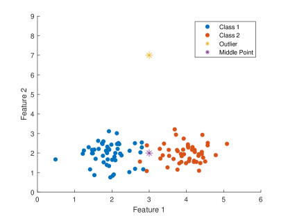
Figure 1: Example to illustrate differences between possibilistic and probabilistic weight assignments.

The Possibilistic Fuzzy Local Information C-Means (PFLICM) [13] and Possibilistic $K$-Nearest Neighbors (P$K$NN) [19] algorithms both use possibility theory and have shown success in various applications. PFLICM has shown success in distinguishing seafloor textures [13, 14] while P$K$NN has been used in landmine detection [19]. Both of these possibilistic approaches could be extended to improve ATR for SAS imagery by providing soft labels that characterize the contents of the seafloor texture. The soft labels could then be used by other algorithms that use seafloor texture information to improve their performance.

In the two previous works that use PFLICM on SAS data, Zare et al 2017 paper [13] and Peeples et al 2018 paper [14], PFLICM was applied in an unsupervised manner, and worked well in that situation. However, in the environmental context problem, it is sometimes good to know what exactly each cluster represents. In this way, a separate ATR pipeline could be implemented for each of the known environments detected. For this reason, PFLICM has been modified in this paper to allow semi-supervised learning to occur for the purpose of explicitly labelling each of the learned cluster centers. In this paper, P$K$NN will be used to segment SAS imagery and be compared with PFLICM for that task. The PFLICM and P$K$NN algorithms are detailed in Sections 2.1 and 2.2 respectively.

2 METHODS

2.1 PFLICM

The Possibilistic Fuzzy Local Information C-Means (PFLICM) algorithm integrates two previous clustering algorithms, Fuzzy Local Information C-Means (FLICM)[20] and Possibilisitic Fuzzy C-Means (PFCM)[21]. The objective function for PFLICM is shown in (1):

$$J=\sum_{c=1}^{C}\sum_{n=1}^{N}a{u_{cn}^{m}\big{(}{||\textbf{x}_{n}-\textbf{c}_{c}||}^{2}_{2}}+G_{cn}\big{)}+bt_{cn}^{q}{||\textbf{x}_{n}-\textbf{c}_{c}||^{2}_{2}}+\sum_{c=1}^{C}\gamma_{c}\sum_{n=1}^{N}\big{(1-t_{cn})}^{q},$$ (1)

with the following constraints

$$u_{cn}\geq 0\hskip 28.45274pt\forall n=1,...,N\hskip 28.45274pt\sum_{c=1}^{C}u_{cn}=1,$$ (2)

where $u_{cn}$ is the membership of the $n^{th}$ pixel in the $c^{th}$ cluster, $\textbf{x}_{n}$ is a $d\times 1$ vector for the nth pixel, $\textbf{c}_{c}$ is a $d\times 1$ vector of the $c^{th}$ cluster, $t_{cn}$ is the typicality value of the $n^{th}$ pixel in the $c^{th}$ cluster, $a$, $b$ and $\gamma_{c}$ are weights on the membership and typicality terms respectively, and $m$ and $q$ control the degree of the membership values for each cluster and identification of outliers in the data respectively. The $G_{cn}$ term follows from Krinidis[20] and incorporates local spatial information:

$$G_{cn}=\underset{k\neq n}{\sum_{{k\in\mathcal{N}_{n}}}}\frac{1}{d_{nk}+1}\big{(}1-u_{ck})^{m}||\textbf{x}_{k}-\textbf{c}_{c}||^{2}_{2},$$ (3)

where $\textbf{x}_{n}$ is the center pixel of a local window, $\mathcal{N}_{n}$ is the neighborhood around the center pixel, and $d_{nk}$ is the Euclidean distance between the center pixel and one of the neighboring pixels ($\textbf{x}_{k}$). The objective function is comprised of fuzzy membership and typicality terms. For the fuzzy membership terms, $\sum_{c=1}^{C}\sum_{n=1}^{N}a{u_{cn}^{m}\big{(}{||\textbf{x}_{n}-\textbf{c}_{c}||}^{2}_{2}}+G_{cn}\big{)}$, the membership of a data point will be higher to cluster centers that are closer (i.e. ${||\textbf{x}_{n}-\textbf{c}_{c}||}^{2}_{2}$ is small). The $G_{cn}$ term encourages neighboring pixels to have similar membership values by incorporating local spatial information (i.e. $d_{nk}$) and also serves as a penalty in the objective function. If the pixels are close (i.e. $d_{nk}$ is small) and membership is low, the $G_{cn}$ term will be large. If a neighbor is far away (i.e. $d_{nk}$ is large), the $G_{cn}$ value of that pixel should be small resulting in a small contribution to the overall objective function. Also, if the neighbors have high membership values, the $G_{cn}$ term will also be small and have little influence on the objective function. Similarly, the typicality terms, $bt_{cn}^{q}{||\textbf{x}_{n}-\textbf{c}_{c}||^{2}_{2}}+\sum_{c=1}^{C}\gamma_{c}\sum_{n=1}^{N}\big{(1-t_{cn})}^{q}$, follow the same principle. The typicality of a data point will be higher to cluster centers that are close. The only difference is that the typicality values do not have the sum to one constraint. This is useful in the identification of new texture types because the typicality of a given data point will be low in all clusters.

The cluster centers, membership and typicality values are updated by alternating optimization. After random initialization, the partial derivative with respect to the $\textbf{c}_{c}$, $u_{cn}$, and $t_{cn}$ is calculated. After setting each expression equal to 0, the following update equations are obtained. For the update equation for the membership values, a Lagrange multiplier term was added to enforce the sum-to-one constraint:

$$\textbf{c}_{c}=\sum_{n}\cfrac{\big{(}au_{cn}^{m}+bt_{cn}^{q}\big{)}\textbf{x}_{n}}{\big{(}au_{cn}^{m}+bt_{cn}^{q}\big{)}},$$ (4)

$$u_{cn}=\cfrac{1}{\sum_{k=1}^{C}\bigg{(}\cfrac{(\textbf{x}_{n}-\textbf{c}_{c})(\textbf{x}_{n}-\textbf{c}_{c})^{T}+G_{cn}}{(\textbf{x}_{n}-\textbf{c}_{k})(\textbf{x}_{n}-\textbf{c}_{k})^{T}+G_{kn}}\bigg{)}},$$ (5)

$$t_{cn}=\cfrac{1}{1+\bigg{(}\frac{b}{\gamma_{c}}||\textbf{x}_{k}-\textbf{c}_{c}||^{2}_{2}\bigg{)}^{\frac{1}{q-1}}},$$ (6)

$\gamma_{c}$ is the mean of the separation of all the data points in the corresponding cluster ($||\textbf{x}_{k}-\textbf{c}_{c}||^{2}_{2}$). The fuzzy factor term, $G$, is treated as a constant in the membership update equation[22]. PFLICM produces membership, typicality and cluster center values for the SAS imagery. The clusters centers can be assigned meaningful labels after clustering the “training” images and then used to compute membership and typicality values for new or “test” SAS images. The semi-supervised PFLICM extension is shown in Figure 2.

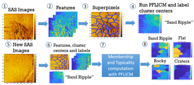
Figure 2: PFLICM: Creating Environmental Context

2.2 PKNN

Possibilistic $K$ Nearest Neighbors[19] extends the traditional $K$-Nearest Neighbors[23] approach to return typicalities for each class instead of crisp labels. The biggest difference comes during the initialization of P$K$NN. Here, a fuzzy membership is assigned to each sample in the training data, this weight takes the form

$$\tilde{\mu}^{i}(y)=\left\{\begin{matrix}0.51+\left(\frac{n_{i}}{K}\right)\times 0.49,&i=j\\ \left(\frac{n_{i}}{K}\right)\times 0.49,&i\neq j\end{matrix}\right..$$ (7)

Where $\tilde{\mu}(y)$ is the fuzzy membership of sample $y$, $j$ represents the actual class label of sample $y$, $i$ is the class for which the current fuzzy weight is being calculated for, and $n_{i}$ represents the number of $K$ nearest samples belonging to class $i$.

In particular, instead of choosing the most often occurring class label in the $K$ nearest training samples, P$K$NN assigns a typicality computed as

$$\text{Conf}^{i}(x^{*})=\frac{1}{K}\sum\limits_{k=1}^{K}\tilde{\mu}^{i}(y_{k})w_{p}(x^{*},y_{k}),$$ (8)

where Conf^$i$($x^{*}$) is the confidence that the current test point, $x^{*}$, belongs to the i^th class in the training data and $y_{k}$ is the $k^{\text{th}}$ nearest training sample.

The function $w_{p}(x,y_{k})$ defines the possibilistic weight of each training sample for the given test point and is related to the distance between the test point and each of the $k$ nearest neighbors. In particular the weight is calculated as

$$w_{p}(x,y_{k})=\left(1+\max(0,\|x-y_{k}\|-\eta)^{2/(m-1)}\right)^{-1},$$ (9)

where $w_{p}$ is the possibilistic weight for each class, $m\in(1,\infty)$ controls the fuzziness of the weight function, and $\eta$ controls how much data is considered to be very close to the test sample. Note that this weight function does not depend on the class label of the training samples and is used instead to determine how important each training sample is in determining the correct label for x. This algorithm returns a confidence value for each class in the training data. These values do not sum to one, which allows points that belong to no class to be assigned low confidence values in every class. In contrast to PFLICM where the cluster centers are assigned labels, each superpixel of the training data is given a label. The P$K$NN segmentation process is shown in Figure 3.

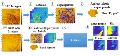
Figure 3: P$K$NN: Creating Environmental Context

3 EXPERIMENTAL RESULTS

The experimental design for our evaluation of each algorithm is as follows: a dataset of 98 SAS images was used and three fold cross validation was performed. Folds two and three contained 33 images while fold one had 32 images. The classes represented in the dataset were sand ripples, flat, rocky, and craters. Before applying PFLICM and P$K$NN to each SAS image, feature extraction and superpixel segmentation were implemented. For each image, a 34 dimensional feature vector was computed using Sobel features[19] (eight edge orientations and square mask sizes five, nine, eleven and fifteen) and lacunarity[24] (window sizes of [31,21] and [21,11]) to aid in capturing texture information. After the features are extracted, superpixels are computed on the grayscale image. Superpixels are pixels that are grouped together based on shared characteristics such as proximity, similarity, good continuation and other metrics[25]. Superpixel segmentation reduces computational costs because an algorithm can be applied at the superpixel level as opposed to each individual pixel. The fast normalized cuts with linear constraints algorithm was used for superpixel segmentation[26]. Once the superpixels are computed, the feature vectors of each pixel that correspond to a given superpixel are averaged. The resulting mean feature vector is assigned as the feature vector of the superpixel. Once the features and superpixels are computed, PFLICM and P$K$NN are applied to each feature vector at the superpixel level.

The parameters were determined manually for each algorithm. For PFLICM, the parameters were set to the following: membership weight $a$ = 14, typicality weight $b$ = 1.4, fuzzifier for fuzzy clustering term $m$ = 1.8, fuzzifier for possibilistic clustering term $q$ = 2.8, and number of clusters = 4. For P$K$NN, the parameters were to set the following: number of neighbors $k$ = 6, fuzzifier for weight term $m$= 2, and value to determine an outlier $\eta$ = 0.01. In order to perform a quantitative assessment of performance, crisp labels were assigned to each superpixel in the ground truth. The class with the maximum typicality values (for P$K$NN) and product of typicality and membership values (for PFLICM) were assigned to the superpixel as a predicted label. The confusion matrices for each fold are shown in Figure 4. The segmentation results of each algorithm are shown in Figure 5 through 10. The product maps are shown for PFLICM and the typicality maps for P$K$NN.

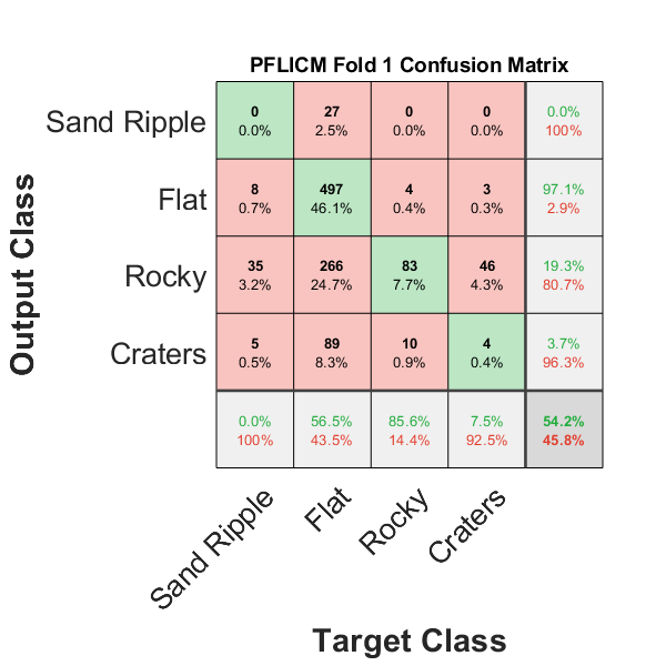
(a) PFLICM Fold One

(b) PFLICM Fold Two

(c) PFLICM Fold Three

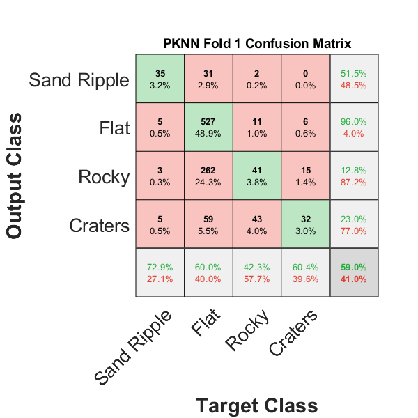
(d) $P$KNN Fold One

(e) $P$KNN Fold Two

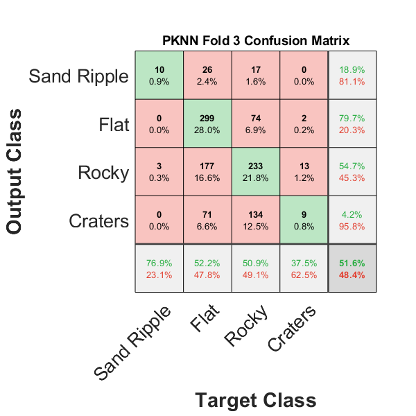
(f) $P$KNN Fold Three

Figure 4: Confusion matrices of PFLICM (4(a)-4(c)) and P$K$NN (4(d)-4(f)) on folds one, two and three respectively.

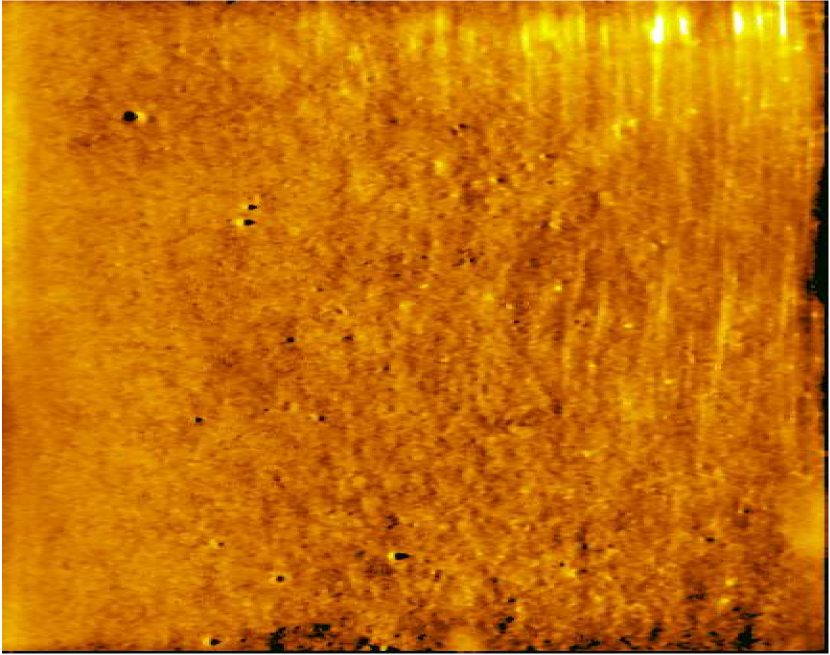
(a) Original image

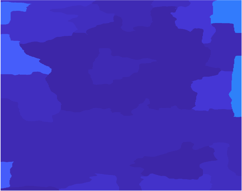
(b) PFLICM - Crater

(c) PFLICM - Flat

(d) PFLICM - Ripples

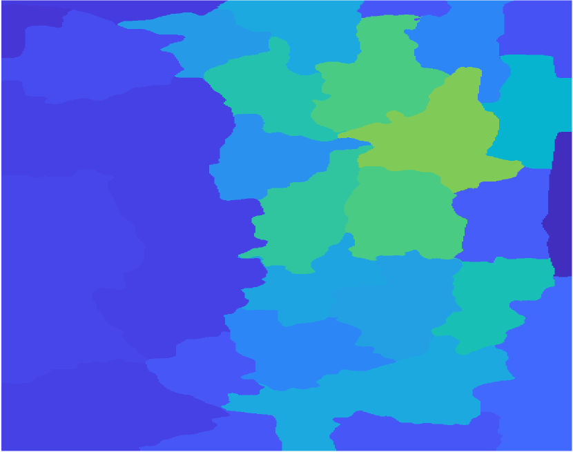
(e) PFLICM - Rocky

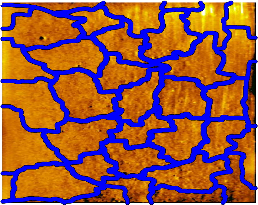
(f) Superpixels

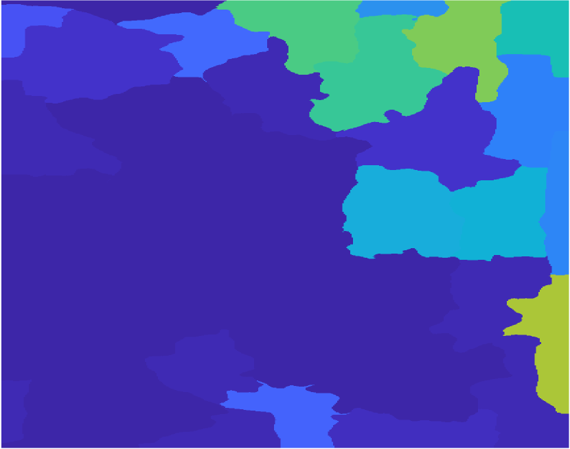
(g) P$K$NN - Crater

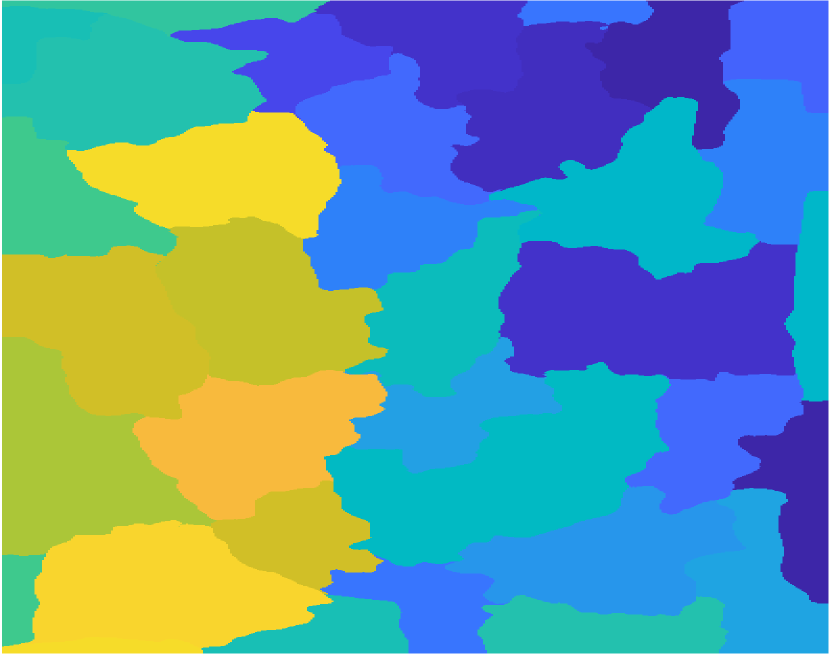
(h) P$K$NN - Flat

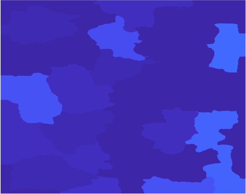
(i) P$K$NN - Ripples

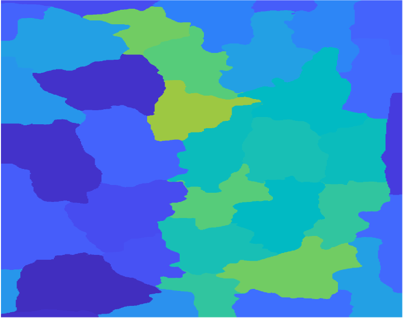
(j) P$K$NN - Rocky

Figure 5: Example image one from fold one. The first column is actual image and superpixel segmentation. Of the remaining columns, the top row is PFLICM product maps and the bottom row is P$K$NN typicality maps.

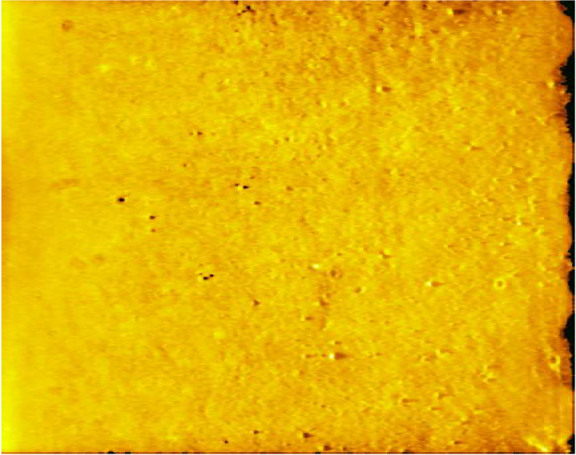
(a) Original image

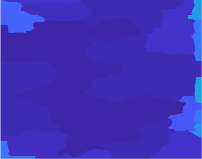
(b) PFLICM - Crater

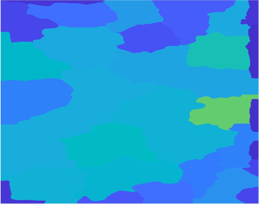
(c) PFLICM - Flat

(d) PFLICM - Ripples

(e) PFLICM - Rocky

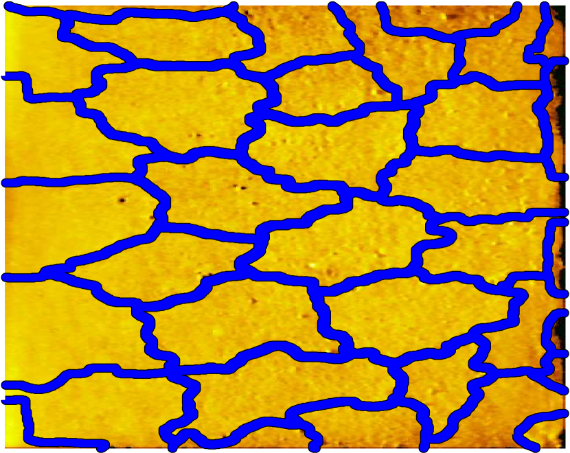
(f) Superpixels

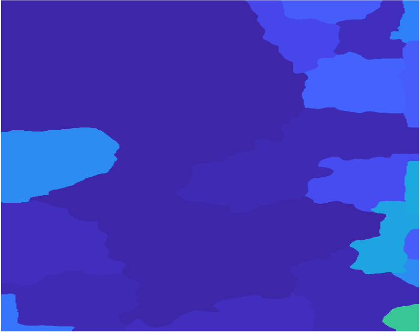
(g) P$K$NN - Crater

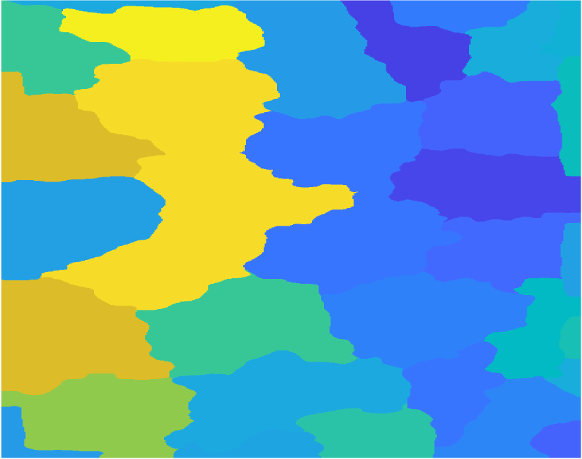
(h) P$K$NN - Flat

(i) P$K$NN - Ripples

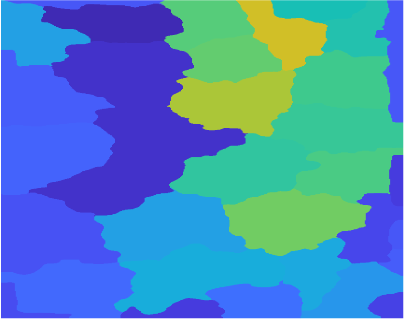
(j) P$K$NN - Rocky

Figure 6: Example image two from fold one. The first column is actual image and superpixel segmentation. Of the remaining columns, the top row is PFLICM product maps and the bottom row is P$K$NN typicality maps.

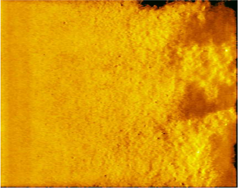
(a) Original image

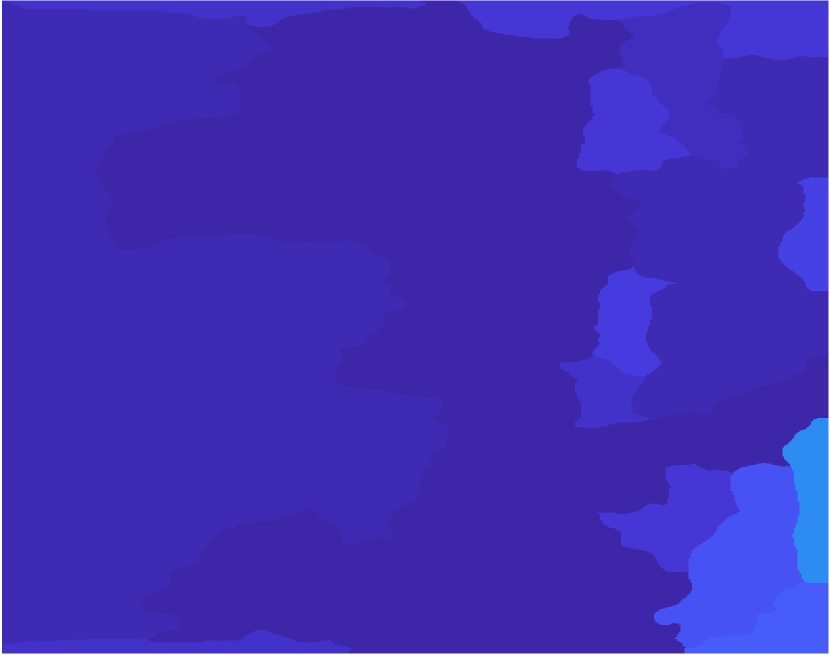
(b) PFLICM - Crater

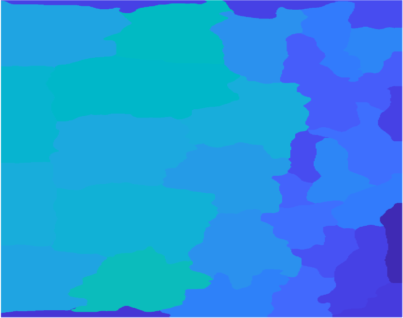
(c) PFLICM - Flat

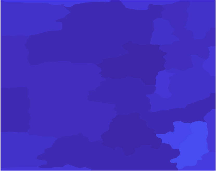
(d) PFLICM - Ripples

(e) PFLICM - Rocky

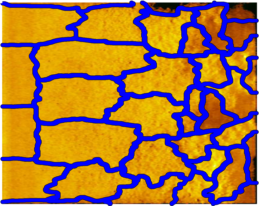
(f) Superpixels

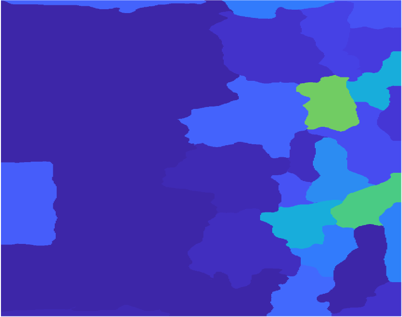
(g) P$K$NN - Crater

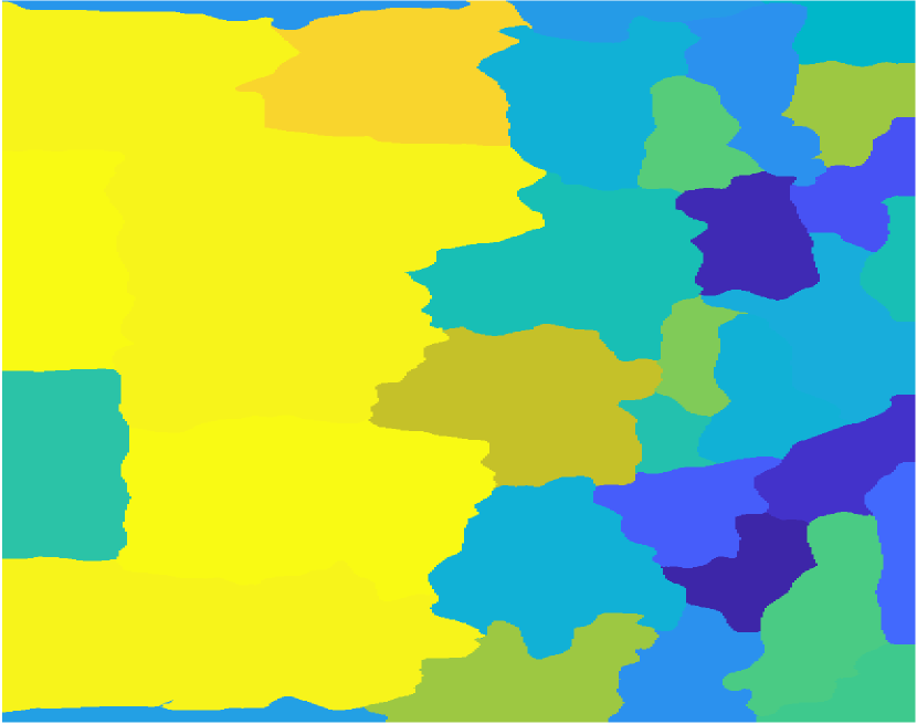
(h) P$K$NN - Flat

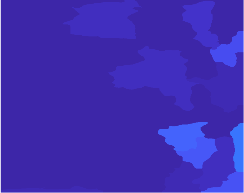
(i) P$K$NN - Ripples

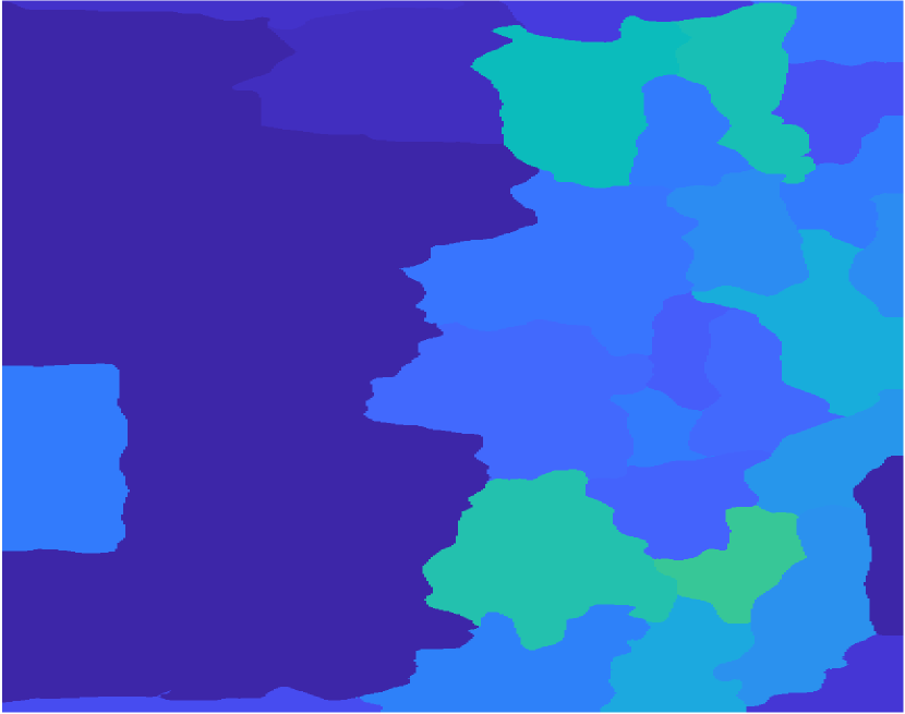
(j) P$K$NN - Rocky

Figure 7: Example image one from fold two. The first column is actual image and superpixel segmentation. Of the remaining columns, the top row is PFLICM product maps and the bottom row is P$K$NN typicality maps.

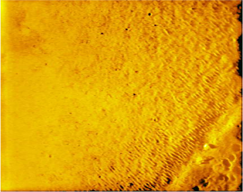
(a) Original image

(b) PFLICM - Crater

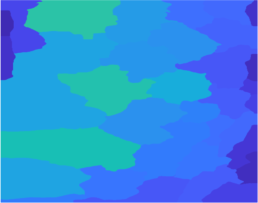
(c) PFLICM - Flat

(d) PFLICM - Ripples

(e) PFLICM - Rocky

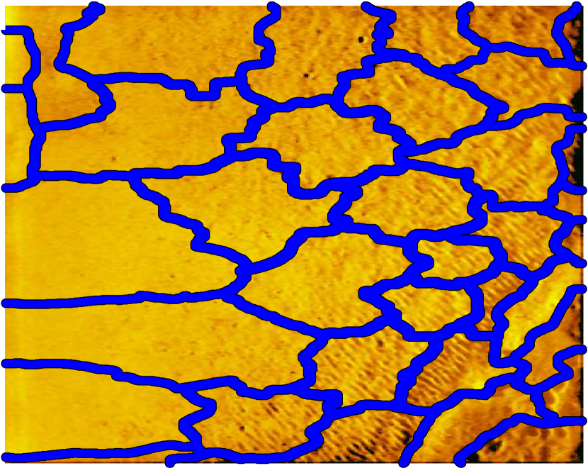
(f) Superpixels

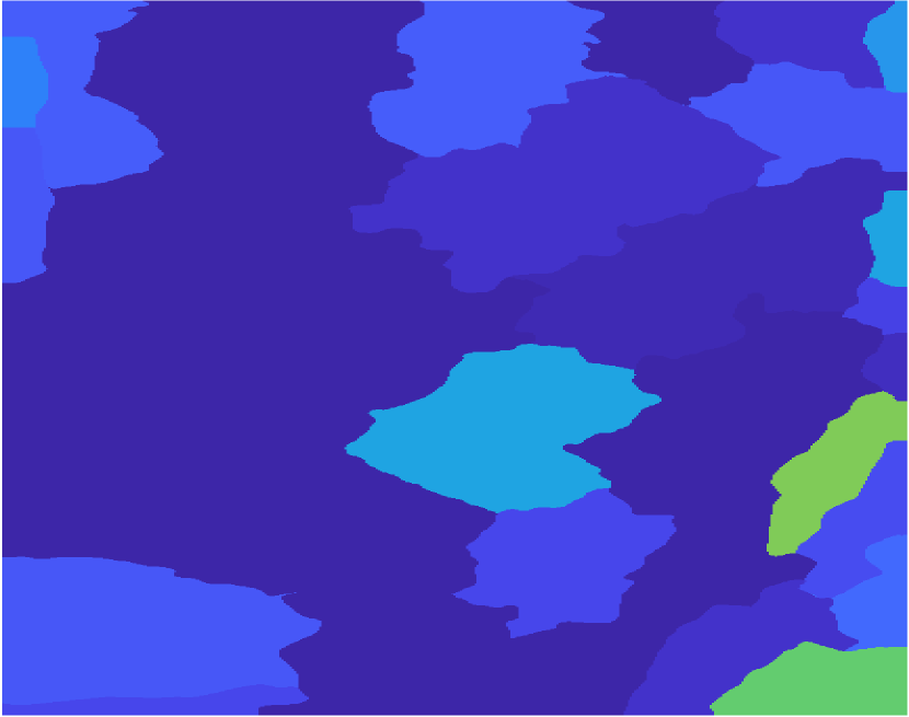
(g) P$K$NN - Crater

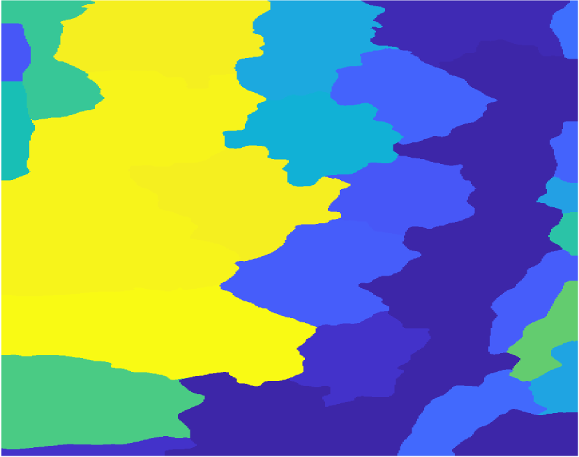
(h) P$K$NN - Flat

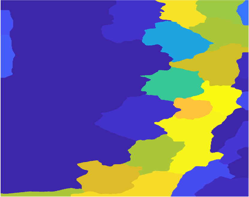
(i) P$K$NN - Ripples

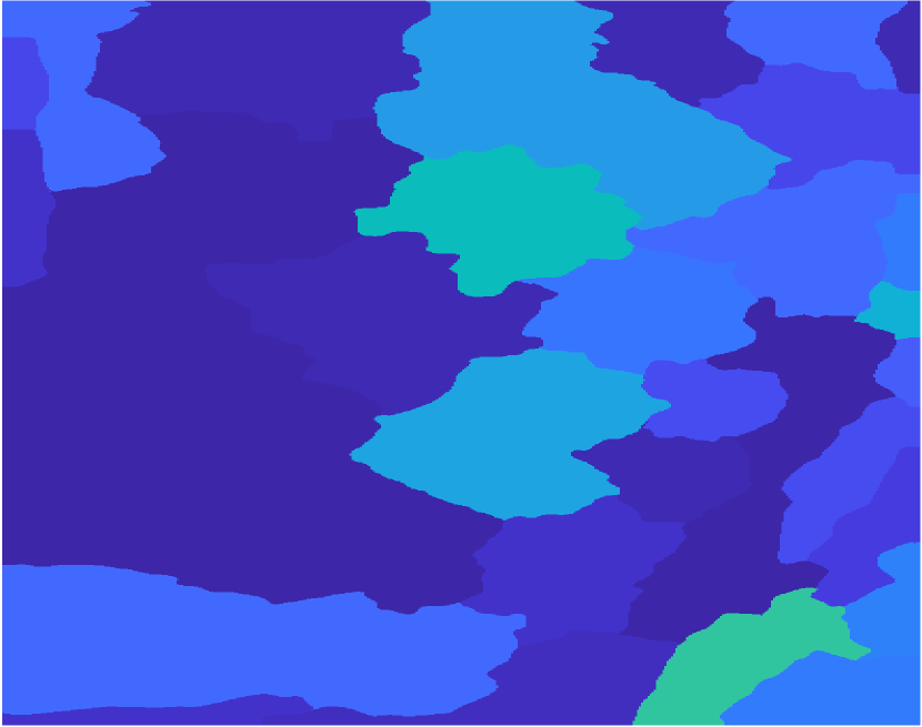
(j) P$K$NN - Rocky

Figure 8: Example image two from fold two. The first column is actual image and superpixel segmentation. Of the remaining columns, the top row is PFLICM product maps and the bottom row is P$K$NN typicality maps.

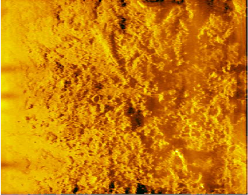
(a) Original image

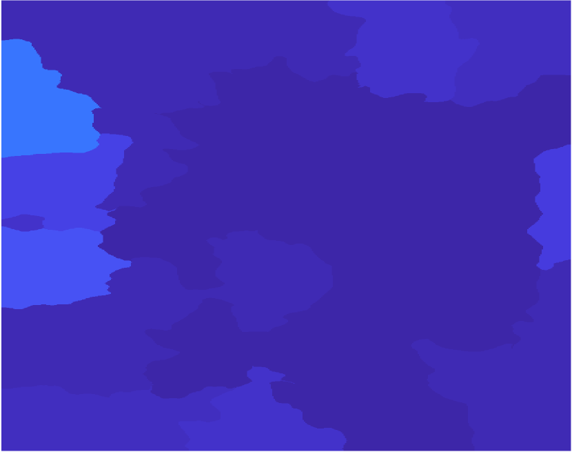
(b) PFLICM - Crater

(c) PFLICM - Flat

(d) PFLICM - Ripples

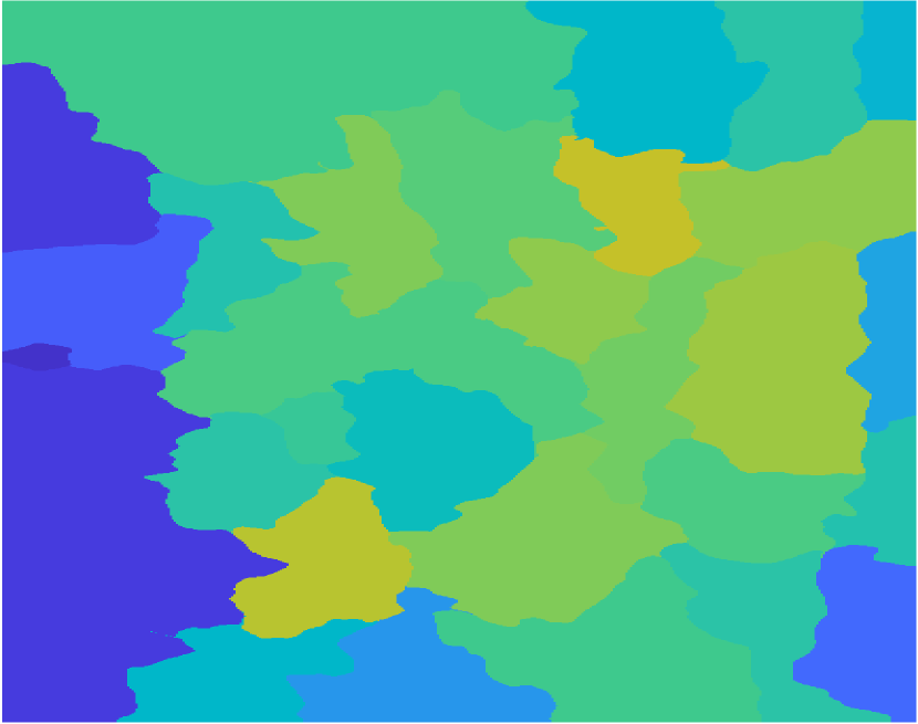
(e) PFLICM - Rocky

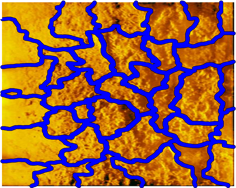
(f) Superpixels

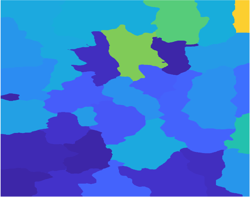
(g) P$K$NN - Crater

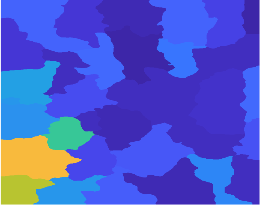
(h) P$K$NN - Flat

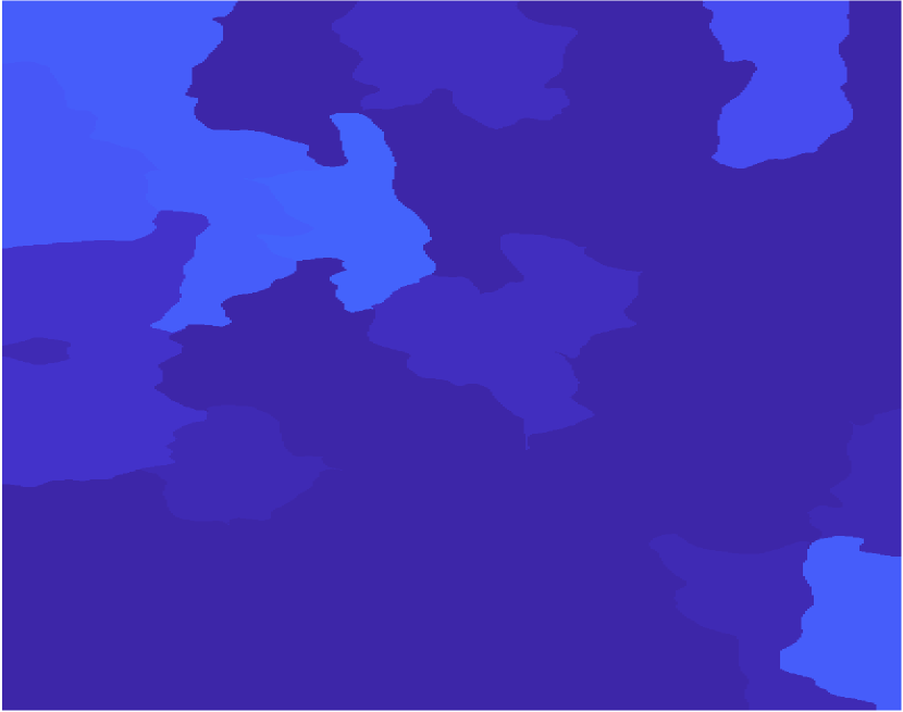
(i) P$K$NN - Ripples

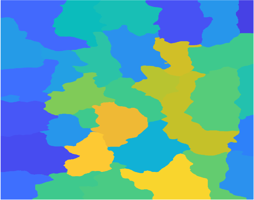
(j) P$K$NN - Rocky

Figure 9: Example image one from fold three. The first column is actual image and superpixel segmentation. Of the remaining columns, the top row is PFLICM product maps and the bottom row is P$K$NN typicality maps.

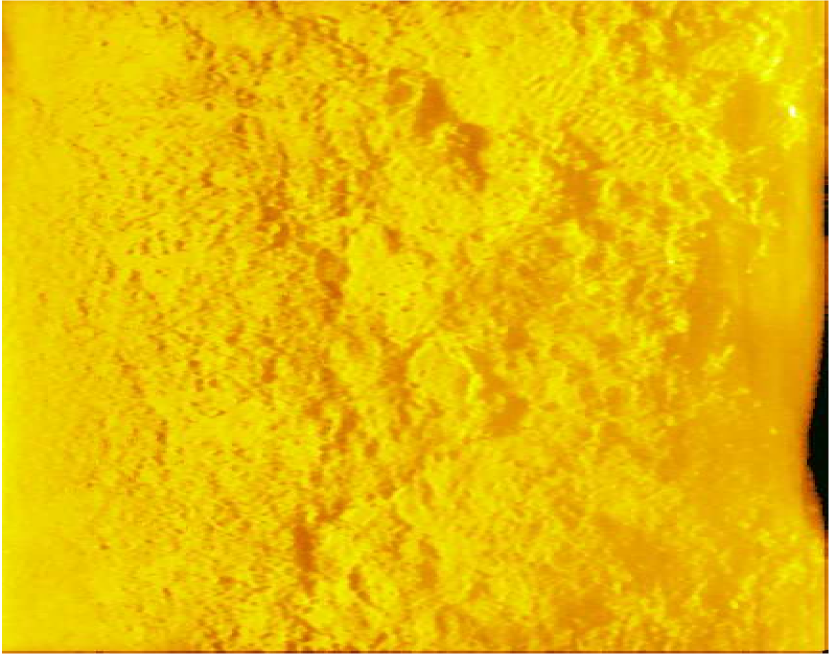
(a) Original image

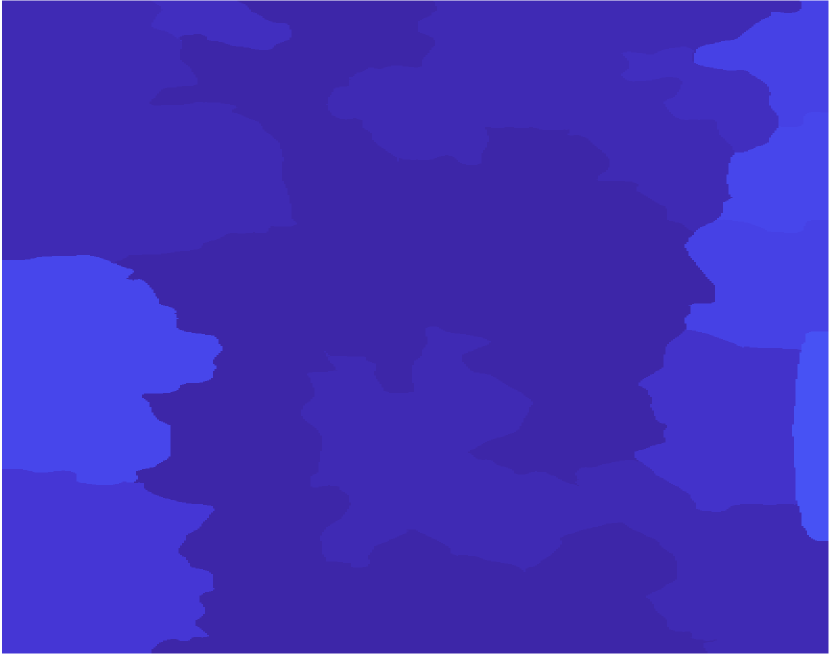
(b) PFLICM - Crater

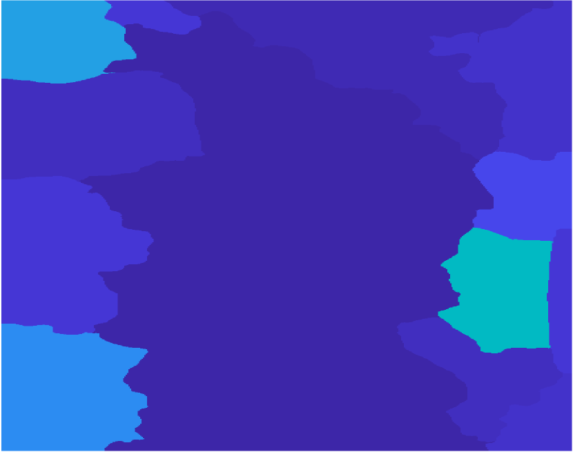
(c) PFLICM - Flat

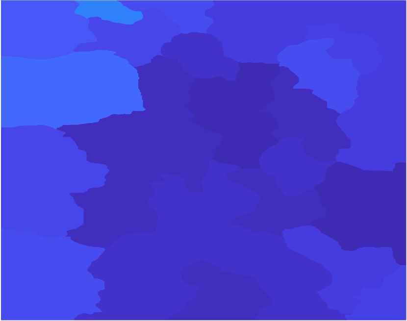
(d) PFLICM - Ripples

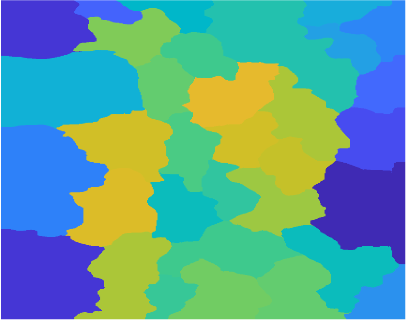
(e) PFLICM - Rocky

(f) Superpixels

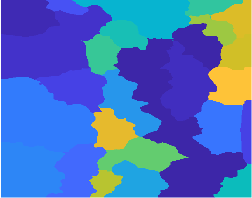
(g) P$K$NN - Crater

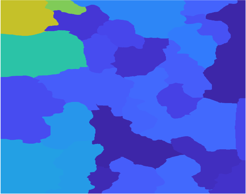
(h) P$K$NN - Flat

(i) P$K$NN - Ripples

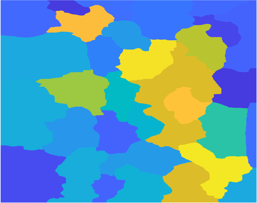
(j) P$K$NN - Rocky

Figure 10: Example image two from fold three. The first column is actual image and superpixel segmentation. Of the remaining columns, the top row is PFLICM product maps and the bottom row is P$K$NN typicality maps.

4 Discussion

Each algorithm achieves comparable performance both qualitatively and quantitatively across each fold. In the segmentation maps (Figures 5 through 10), PFLICM and P$K$NN partitions are very similar to one another. The P$K$NN typicality maps had higher responses than the product maps from PFLICM for correctly identified textures. A possible reason for this is that P$K$NN was designed as a classifier while PFLICM is a clustering method. P$K$NN will discriminate between the textures at higher responses while PFLICM only groups areas of the image that are similar, resulting in less distinctive segments of textures.

From the confusion matrices in Figure 4, both PFLICM and P$K$NN perform the best on flat textures. A majority of the SAS images chosen in each fold contained a majority of superpixels in flat regions of the seafloor so the result is as expected since most of the training data is comprised of this class. Both algorithms did not perform as well on craters due to there being few superpixels containing pure crater regions. In future work, expanding the dataset to be more representative of each class could help mitigate some of the difference across each texture. Also, both algorithms perform soft classification so using “crisp” metrics such as accuracy, precision, and recall from a confusion matrix may not be the best way to quantitatively evaluate segmentation. However, this lays a baseline for a measurable comparison of PFLICM and P$K$NN.

Another metric used for comparison was the computational efficiency of each algorithm. For training, the time complexity for PFLICM and P$K$NN are $O(mc^{2}i)$ and $O(mlog^{2}(m)+mklog(m)+mlk)$ respectively ($m$ is the number of training samples, $c$ is the number of clusters, $i$ is the number of iterations, $k$ is the number of neighbors, and $l$ is the number of classes). For testing, the time complexity for PFLICM and P$K$NN are $O(nc^{2})$ and $O(nklog(m)+nlk)$ respectively ($n$ is the number of testing samples). The terms $c$ and $k$ are mostly negligable since for most cases $c,k<<m,n$, thus leaving the amount of training and testing as the dominant factors. The logarithmic terms in the P$K$NN complexity come from the use of a kd-tree [27] for calculating the nearest neighbors. From these complexities it can be seen that both algorithms scale linearly with the number of training and testing samples meaning that both algorithms could be effectively used with large amounts of testing data, with some limitations for P$K$NN. However, PFLICM does scale better since the testing complexity does not rely on the number of training samples. This implies that PFLICM could use a much larger training set and not impact testing time, whereas the testing phase of P$K$NN scales logarithmically with the size of the training set.

The labelling cost of each algorithm is another source of comparison for analysis. The P$K$NN does require that the training data is labelled at the superpixel level while PFLICM only requires labels assigned to each cluster center after training is completed. Despite increased labelling expense, P$K$NN will be more effective against poor labelling. P$K$NN computes possibilistic weights for each of the neighbors and these weights determine the level of importance each neighbor will have in the class confidences of a test sample despite the class label associated with each superpixel. For PFLICM, there is no mechanism in place to account for wrong labels on the cluster center level. As a result, P$K$NN accounts for errors made during labelling which is a desirable property for the segmentation process.

5 CONCLUSION

A comparison of PFLICM and P$K$NN are presented in this work. The performance of both algorithms is comparable to one another, both quantitatively and qualitatively. P$K$NN is significantly less computationally expensive than PFLICM in training as the training dataset increases, but PFLICM can have a much lower testing complexity if the training set is very large. P$K$NN also has an advantage over PFLICM in that P$K$NN can account for poor labelling that may occur within the training data. In future work, P$K$NN can be used to identify new textures in images through the possibilistic aspect. If the typicality values are low for each class, a new texture type can be identified. In order to add new seafloor types, a streaming/sequential clustering approach could be used[28]. For an ATR system, the typicality values of P$K$NN could serve as environmental weights to assist in the classification of targets and create the environmental context for ATR applications.

- [1] Bhanu, B., “Automatic target recognition: State of the art survey,” IEEE transactions on aerospace and electronic systems (4), 364–379 (1986).
- [2] Roth, M. W., “Survey of neural network technology for automatic target recognition,” IEEE Transactions on neural networks 1(1), 28–43 (1990).
- [3] Del Rio Vera, J., Coiras, E., Groen, J., and Evans, B., “Automatic target recognition in synthetic aperture sonar images based on geometrical feature extraction,” EURASIP Journal on Advances in Signal Processing 2009, 14 (2009).
- [4] Williams, D. P. and Fakiris, E., “Exploiting environmental information for improved underwater target classification in sonar imagery,” IEEE Transactions on Geoscience and Remote Sensing 52(10), 6284–6297 (2014).
- [5] Groen, J., Coiras, E., Vera, J. D. R., and Evans, B., “Model-based sea mine classification with synthetic aperture sonar,” IET radar, sonar & navigation 4(1), 62–73 (2010).
- [6] Lyons, P., Suen, D., Galusha, A., Zare, A., and Keller, J., “Comparison of prescreening algorithms for target detection in synthetic aperture sonar imagery,” in [Detection and Sensing of Mines, Explosive Objects, and Obscured Targets XXIII ], 10628, 1062811, International Society for Optics and Photonics (2018).
- [7] Hayes, M. P. and Gough, P. T., “Synthetic aperture sonar: a review of current status,” IEEE Journal of Oceanic Engineering 34(3), 207–224 (2009).
- [8] Zare, A. and Gader, P., “Context-based endmember detection for hyperspectral imagery,” in [1st IEEE Workshop on Hyperspectral Image and Signal Processing: Evolution in Remote Sensing (WHISPERS) ], (Aug. 2009).
- [9] Du, X., Zare, A., and Cobb, J. T., “Possibilistic context identification for sas imagery,” in [Proc. SPIE 9454, Detection and Sensing of Mines, Explosive Objects, and Obscured Targets XX ], 9454 (May 2015).
- [10] Liu, T., Abd-Elrahman, A., Zare, A., Dewitt, B., Flory, L., and Smith, S., “A fully learnable context-driven object-based model for mapping land cover using multi-view data from unmanned aircraft systems,” Remote Sensing of Environment 216, 328–344 (Oct. 2018).
- [11] Williams, D. P., “Bayesian data fusion of multiview synthetic aperture sonar imagery for seabed classification,” IEEE Transactions on Image Processing 18(6), 1239–1254 (2009).
- [12] Fandos, R., Sadamori, L., and Zoubir, A. M., “High quality segmentation of synthetic aperture sonar images using the min-cut/max-flow algorithm,” in [2011 19th European Signal Processing Conference ], 51–55, IEEE (2011).
- [13] Zare, A., Young, N., Suen, D., Nabelek, T., Galusha, A., and Keller, J., “Possibilistic fuzzy local information c-means for sonar image segmentation,” IEEE Symposium Series on Computational Intelligence (SSCI) Proceedings (2017).
- [14] Peeples, J., Suen, D., Zare, A., and Keller, J., “Possibilistic fuzzy local information c-means with automated feature selection for seafloor segmentation,” in [Detection and Sensing of Mines, Explosive Objects, and Obscured Targets XXIII ], 10628, 1062812, International Society for Optics and Photonics (2018).
- [15] Zadeh, L. A., “Fuzzy sets as a basis for a theory of possibility,” Fuzzy sets and systems 1(1), 3–28 (1978).
- [16] Krishnapuram, R. and Keller, J. M., “A possibilistic approach to clustering,” IEEE transactions on fuzzy systems 1(2), 98–110 (1993).
- [17] Zhang, J.-S. and Leung, Y.-W., “Improved possibilistic c-means clustering algorithms,” IEEE Transactions on Fuzzy Systems 12(2), 209–217 (2004).
- [18] Jenhani, I., Amor, N. B., and Elouedi, Z., “Decision trees as possibilistic classifiers,” International Journal of Approximate Reasoning 48(3), 784–807 (2008).
- [19] Frigui, H. and Gader, P., “Detection and discrimination of land mines in ground-penetrating radar based on edge histogram descriptors and a possibilistic -nearest neighbor classifier,” IEEE Transactions on Fuzzy Systems 17(1), 185–199 (2009).
- [20] Krinidis, S. and Chatzis, V., “A robust fuzzy local information c-means clustering algorithm,” IEEE transactions on image processing 19(5), 1328–1337 (2010).
- [21] Pal, N. R., Pal, K., Keller, J. M., and Bezdek, J. C., “A possibilistic fuzzy c-means clustering algorithm,” IEEE transactions on fuzzy systems 13(4), 517–530 (2005).
- [22] Celik, T. and Lee, H. K., “Comments on “a robust fuzzy local information c-means clustering algorithm”,” IEEE Transactions on Image Processing 22(3), 1258–1261 (2013).
- [23] Cover, T. M., Hart, P. E., et al., “Nearest neighbor pattern classification,” IEEE transactions on information theory 13(1), 21–27 (1967).
- [24] Williams, D. P., “Fast unsupervised seafloor characterization in sonar imagery using lacunarity,” IEEE transactions on Geoscience and Remote Sensing 53(11), 6022–6034 (2015).
- [25] Ren, X. and Malik, J., “Learning a classification model for segmentation,” in [null ], 10, IEEE (2003).
- [26] Xu, L., Li, W., and Schuurmans, D., “Fast normalized cut with linear constraints,” in [2009 IEEE Conference on Computer Vision and Pattern Recognition ], 2866–2873, IEEE (2009).
- [27] Bentley, J. L., “Multidimensional binary search trees used for associative searching,” Commun. ACM 18, 509–517 (Sept. 1975).
- [28] Ackerman, M. and Dasgupta, S., “Incremental clustering: The case for extra clusters,” in [Advances in Neural Information Processing Systems ], 307–315 (2014).