Quantum 4d Yang-Mills Theory and
Time-Reversal Symmetric
5d Higher-Gauge Topological Field Theory:
Anyonic-String/Brane Braiding Statistics to Link Invariants

Zheyan Wan^1,2,  Juven Wang^3,4, and Yunqin Zheng^5
1Yau Mathematical Sciences Center, Tsinghua University, Beijing 100084, China
²School of Mathematical Sciences, USTC, Hefei 230026, China
³School of Natural Sciences, Institute for Advanced Study, Einstein Drive, Princeton, NJ 08540, USA
⁴Center of Mathematical Sciences and Applications, Harvard University, Cambridge, MA 02138, USA
⁵Physics Department, Princeton University, Princeton, New Jersey 08544, USA

We explore various 4d Yang-Mills gauge theories (YM) living as boundary conditions of 5d gapped short/long-range entangled (SRE/LRE) topological states. Specifically, we explore 4d time-reversal symmetric pure YM of an SU(2) gauge group with a second-Chern-class topological term at $\theta=\pi$ (SU(2)_θ=π YM), by turning on the background fields for both the time-reversal (i.e., on unorientable and non-spin manifolds) and the 1-form center global symmetry. We find Four Siblings of time-reversal and Lorentz symmetry-enriched SU(2)_θ=π YM with distinct couplings to background fields, labeled by $(K_{1},K_{2})$: $K_{1}=0,1$ specifies Kramers singlet/doublet Wilson line and new mixed higher ’t Hooft anomalies; $K_{2}=0,1$ specifies boson/fermionic Wilson line and a new Wess-Zumino-Witten-like counterterm. Higher anomalies indicate that in order to realize all higher $n$-global symmetries locally on $n$-simplices, the 4d theory becomes a boundary of a 5d higher-symmetry-protected topological state (SPTs, as an invertible topological quantum field theory (iTQFT) or a cobordism invariant in math, or as a 5d higher-symmetric interacting topological superconductor in condensed matter). Via Weyl’s gauge principle, by dynamically gauging the 1-form symmetry, we transform a 5d bulk SRE SPTs into an LRE symmetry-enriched topologically ordered state (SETs); thus we obtain the 4d SO(3)_θ=π YM-5d LRE-higher-SETs coupled system with dynamical higher-form gauge fields. We further derive new exotic anyonic statistics of extended objects such as 2d worldsheet of strings and 3d worldvolume of branes, physically characterizing the 5d SETs. We discover triple and quadruple link invariants potentially associated with the underlying 5d higher-gauge TQFTs, hinting at a new intrinsic relation between non-supersymmetric 4d pure YM and topological links in 5d. We provide 4d-5d lattice simplicial complex regularizations and bridge to 4d SU(2) and SO(3)-gauged quantum spin liquids as 3+1 dimensional realizations. We constrain YM low-energy gauge dynamics by higher anomalies and a higher symmetry-extension method.

1 Introduction and Summary

The world where we reside, to our best present understanding, can be described by quantum theory and the underlying long-range entanglement. Quantum field theory (QFT) and in particular quantum gauge field theory, under the spell of Gauge Principle following the insights since Maxwell, Hilbert, Weyl, Pauli, and others (see a historical review [1]), embodies the quantum, special relativity and long-range entanglement into a systematic framework. Yang-Mills (YM) gauge theory [2], generalizing the U(1) gauge group of quantum electrodynamics to a non-abelian Lie group, has been proven to be powerful to describe the Standard Model physics.

The Euclidean partition function of a pure YM theory with an SU(N) gauge group on a 4-dimensional (i.e., 4d) spacetime $M^{4}$ and a second-Chern-class topological term $S_{\theta}$ labeled by $\theta$, i.e., SU(N)_θ-YM, is

$${\mathbf{Z}}^{\text{$4$d}}_{{\text{YM}}}\equiv\int[{\cal D}{a}]\exp\big{(}-S_{\text{SU(N)}_{\theta}}[a]\big{)}\equiv\\ \int[{\cal D}{a}]\exp\big{(}-S_{\text{SU(N)}_{\theta=0}}[a]\big{)}\exp\big{(}-S_{\theta}[a]\big{)}\equiv\int[{\cal D}{a}]\exp\Bigg{(}-\int\limits_{M^{4}}\frac{1}{g^{2}}\text{Tr}\,F_{a}\wedge\star F_{a}+\int\limits_{M^{4}}\frac{\hskip 1.0pt\mathrm{i}\hskip 1.0pt\theta}{8\pi^{2}}\text{Tr}\,F_{a}\wedge F_{a}\Bigg{)},$$ (1.1)

where $a$ is the ${\rm SU}({\rm N})$ gauge field, $F_{a}=\hskip 1.0pt\mathrm{d}a-\hskip 1.0pt\mathrm{i}\hskip 1.0pta\wedge a$ is the SU(N) field strength, and $g$ is the gauge coupling constant. See the footnote for further explanations of the notations. When $\theta=0$, the SU(N)_θ=0 YM theory is believed to be in the confined phase [3], have an energy gap, and have a single ground state on any manifold. In particular, there is no ’t Hooft anomaly [4]. Recently, Ref. [5] discovered that for SU(N)_θ=π- YM with even N, there is a subtle ’t Hooft anomaly involving the time-reversal symmetry $\mathbb{Z}_{2}^{T}$ and 1-form center global symmetry $\mathbb{Z}_{{\rm N},[1]}^{e}$. The ’t Hooft anomaly of a 4d theory is captured by a 5d topological term through the anomaly inflow mechanism [7]. Schematically, Ref. [5] suggested a 5d topological term linear in the time-reversal background field ${\cal T}$ and quadratic in the $\mathbb{Z}_{{\rm N},[1]}^{e}$ background field $B$,

$$\sim{\cal T}BB.$$ (1.2)

The 5d topological term characterizes the 5d short-rangle-entangled (SRE) phase. See Sec. 2 for more rigorous definitions of the background fields and the 5d topological term.

Further recently, Ref. [8] suggested that there are additional new higher ’t Hooft anomalies for some 4d SU(N)_θ=π theories at even N: From one perspective, Ref. [8] suggested that when ${\rm N}=2$, there is a mixed anomaly captured by a 5d topological term which is cubic in ${\cal T}$ and linear in $B$, which is schematically denoted as

$$\sim{\cal T}{\cal T}{\cal T}B.$$ (1.3)

From another perspective, Ref. [8] suggested that the SU(N)_θ=π YM at an even integer ${\rm N}\geq 4$ contains new mixed anomalies involving $\mathbb{Z}_{2}^{T}$, $\mathbb{Z}_{{\rm N},[1]}^{e}$ and a 0-form charge conjugation (i.e., a $\mathbb{Z}_{2}$ outer-automorphism) symmetry. For example, at N $=4$, another anomaly can be captured by the 5d topological terms schematically as ${\sim A_{C}{\cal T}{\cal T}B.}$ Here $A_{C}$ is a 1-form background field for the 0-form $\mathbb{Z}_{2}^{C}$ charge conjugation symmetry. In the following, we will make the above schematic 5d topological terms Eq. (1.2) and Eq. (1.3) mathematically precise, following the setup in Ref. [8] and Ref. [10].

The above 5d topological terms can be regarded as semi-classical partition functions (definable on closed 5-manifolds with appropriate structures) whose functional values depend on the external values to global symmetry-background probe fields. These 5d topological terms are also known as invertible topological quantum field theories (iTQFTs) in the literatures. In the present work, we will further dynamically gauge the 1-form symmetry $\mathbb{Z}_{{\rm N},[1]}^{e}$ associated to the coupled systems of 4d YM and 5d topological terms above. After gauging $\mathbb{Z}_{{\rm N},[1]}^{e}$, the 5d SRE topological terms become 5d long-range entangled (LRE) topological quantum field theories (TQFT). We further apply the methods developed in Refs. [11, 12, 13] to analytically compute the physical observables of the higher-gauge 5d TQFTs. The physical observables of 5d TQFTs include, for example, (i) the partition functions ${\mathbf{Z}}[M^{5}]$ on closed manifolds $M^{5}$, (ii) braiding statistics of anyonic strings and anyonic branes whose spacetime trajectories forming 2d worldsheets and 3d worldvolumes respectively, and link invariants of these 2d worldsheets and 3d worldvolumes in $M^{5}$. We uncover new spacetime braiding processes and link invariants, including triple and quadruple linkings analogous to previous works [12, 14, 11, 15, 16].

Now let us take a step back to digest the physical meanings of these 5d topological terms Eq. (1.2)-Eq. (1.3). The $d$ dimensional ’t Hooft anomaly of ordinary 0-form global symmetries is known to be captured by a $(d+1)$ dimensional iTQFT. In the condensed matter literatures, these $(d+1)$d iTQFTs describe Symmetry-Protected Topological states (SPTs) [29, 30, 31, 32]. The relations between the SPTs and the response probe field-theoretic partition functions have been systematically studied, selectively, in [33, 21, 34, 35, 36, 37, 38] (and References therein), and climaxed to the hint of cobordism classification of SPTs[39, 40]. Recently the iTQFTs and SPTs are found to be systematically classified by a powerful cobordism theory framework of Freed-Hopkins [41], following the earlier work of Thom-Madsen-Tillmann spectra [42, 43].

Further recently, Ref. [10] generalized the Thom-Madsen-Tillmann-Freed-Hopkins cobordism theory [42, 43, 41] to the cases with generalized higher global symmetries [6]. The generalized cobordism group computation [10], which involves the bordism group of higher classifying spaces and their fibrations, e.g. $\mathrm{B}\mathbb{G}$, can capture the $d$ dimensional higher ’t Hooft anomaly of generalized global symmetries $\mathbb{G}$ by $(d+1)$ dimensional bordism invariants (i.e., generalized symmetric iTQFTs or higher symmetric iTQFTs). In the following, we also call the generalized symmetric iTQFTs as higher-SPTs. The $d$d boundary of $(d+1)$d higher-SPTs has $d$d higher-anomalies. Gauging the higher-symmetry of higher-SPTs gives rise to higher-gauge theories. Earlier pursuits on a systematic framework of the generalized symmetric iTQFTs through cobordism theories and cohomology theories include, but not limited to, Ref. [44, 45, 46, 47, 48, 49, 50, 51, 52, 53] and references therein. In this work, we identify the 4d anomalies of SU(N)_θ=π YM Eq. (1.2)-Eq. (1.3) with the mathematically precise 5d bordism invariants, obtained in Refs. [8] and [10].

Let us rephrase the higher anomalies into a condensed matter language on the lattice: Higher anomaly indicates that in order to realize all higher $n$-global symmetries locally on $n$-simplices, the theory needs to become a boundary of a one-higher dimensional higher-symmetry-protected topological state (higher-SPTs). If a theory has a higher anomaly, then the theory in its own dimension has some higher $n$-global symmetries acting non-locally (on $n$-simplices). Then there is an obstruction to gauge such a non-local symmetry, hence the name of higher (’t Hooft) anomaly [4]. More in Sec. 8.

1.1 The Outline

Here are the outlines of the present work.

$\bullet$ Sec. 2 — We identify the 5d bordism invariants with the ’t Hooft anomalies of 4d SU(N)_θ=π YM theory (where we focus on ${\rm N}=2$), as a version of higher-anomaly matching.

$\bullet$ Sec. 3 — We clarify and enumerate possible distinct classes of 4d SU(2)_θ=π YM theories. We take the condensed matter viewpoint, where we regard the SU(2)_θ=π YM theories as infrared theories emerging from high-energy ultraviolet (UV) bosonic systems with a lattice cutoff, as opposed to fermionic systems. We thus call the UV system as bosonic YM theories. These bosonic YM theories still allow Wilson line operators as worldlines of particles being (1) either bosonic or fermionic in quantum statistics, (2) either Kramers doublet or Kramers singlet under the time-reversal symmetry. This supplements as a partial classification of 4d SU(2)_θ=π bosonic YM theories. We apply the tools in Ref. [38] to understand the relation between gauge bundle constraint and the properties of line/surface operators.

From Sec. 2 and Sec. 3, we will see that there are at least four closely related 4d SU(2)_θ=π non-supersymmetric pure YM theories (which we nickname them as Four Siblings of 4d SU(2)_θ=π YM theories) with bosonic UV completions. Each of them carries either a distinct 4d ’t Hooft anomaly associated with a 5d higher-SPTs or a distinct 4d counterterm. The distinct 5d higher-SPTs labeled by distinct the 5d bordism invariants are actually the physical analogs of the 5d (4+1D) one-form-center-symmetry-protected interacting topological superconductors in the condensed matter language.

$\bullet$ Sec. 4 and Sec. 5 — We dynamically gauge the 1-form center symmetry $\mathbb{Z}_{2,[1]}^{e}$. This turns the 4d SU(2)_θ=π YM/5d-higher-SPTs coupled systems in [8] into 4d SO(3)_θ=π YM/5d-higher-SETs coupled systems, where SETs stand for the symmetry-enriched topologically ordered states. We then explore the detailed properties of various 5d higher-SETs. The 5d higher-SETs are described by 5d time-reversal symmetric higher-TQFTs with emergent 2-form dynamical gauge fields. We mainly focus on the Four Siblings of 5d higher-SETs, while also consider other highly relevant exotic 5d higher-SETs. To characterize these 5d higher-SETs, we study the following aspects:

1. Partition function ${\mathbf{Z}}[M^{5}]$ without extended operator (1-line, 2-surface, 3-submanifold) insertions on 5-manifold $M^{5}$. We compute ${\mathbf{Z}}[M^{5}]$ following the techniques and tools built from [12] and [13]. In particular, when $M^{5}=M^{4}\times S^{1}$, the partition function ${\mathbf{Z}}[M^{4}\times S^{1}]$ is the topological ground state degeneracy (topological GSD) on a spatial $M^{4}$. This issue is addressed in Sec. 4.

2. Braiding statistics involving anyonic 1D string/2D branes, and the associated link invariants of the spacetime 2d worldsheet/3d worldvolume. Here we compute the path integral ${\mathbf{Z}}[M^{5};W,U,\dots]$ with extended-operator insertions ($W,U,\dots$), following the techniques and tools built from [11, 12, 15, 16]. This issue is addressed in Sec. 5.

$\bullet$ Sec. 6 — We provide the exemplary spacetime braiding processes of anyonic string/brane in 5d, and the link configurations of extended operators, which can be detected by the link invariants that we derived in Sec. 5.

$\bullet$ Sec. 7 — We re-examine the coupled system of 4d SO(3)_θ=π YM theories and 5d-higher-SETs appeared in Sec. 4.

$\bullet$ Sec. 8 — We construct the lattice regularization and UV completion of some of our systems. This includes a lattice realization of 5d higher-SPTs and higher-gauge SETs by implementing on 5d simplicial complex spacetime path integral, and a 4+1D “condensed matter” realization on the spatial Hamiltonian operator. We also provide a lattice regularization of (1) higher-symmetry-extended and (2) higher-symmetry-preserving anomalous 3+1D topologically ordered gapped boundaries by generalizing the method of [54]. The higher-symmetry-extension method was also developed in [55].

$\bullet$ Sec. 9 — We conclude and make connections to physics and mathematics in other perspectives.

Before we proceed to the detailed discussions in the main text, we first give a quick overview on more colloquial and pedestrian summaries in terms of schematic descriptions and Table 1, in Sec. 1.2. Readers who are not familiar with certain mathematical information or physical motivations may seek for additional helps from Refs. [38] (and its Appendices), [8] and [10].

1.2 Summaries and Tables

As we mentioned, in Sec. 2 and Sec. 3, we will see that there are at least four closely related 4d SU(2)_θ=π non-supersymmetric pure YM theories (nicknamed the Four Siblings of 4d SU(2)_θ=π YM theories are labeled by $(K_{1},K_{2})\in(\mathbb{Z}_{2},\mathbb{Z}_{2})$) with a bosonic UV completion. They carry either distinct 4d higher ’t Hooft anomalies or distinct 4d counterterms. All these anomalies that we will discuss below are the mod 2 non-perturbative global anomalies, similar to the old and the new SU(2) anomalies [56, 57]; except that instead of an ordinary global symmetry, now we require a higher 1-form symmetry $\mathbb{Z}_{2,[1]}^{e}$ to probe higher anomalies. Here we advertise these results in a colloquial and pedestrian manner.

1. $(K_{1},K_{2})=(0,0)$. The 1st Sibling of 4d SU(2)_θ=π with Kramers singlet ($T^{2}=+1$) bosonic Wilson line has the 4d anomaly/5d bordism invariant schematically as:

   $$\sim w_{1}(TM)BB,$$ (1.4)

   with the $j$-th Stiefel-Whitney (SW) class $w_{j}(TM)$ of spacetime manifold $M$’s tangent bundle $TM$. Here $B\in\operatorname{H}^{2}(M,\mathbb{Z}_{2})$ is a degree-2 cohomology class obtained from restricting the 2-form ${\cal B}$ field via ${\cal B}\sim\pi B$ and $\oint_{\Sigma}{\cal B}=\pi\mathbb{Z}$ for any closed surface $\Sigma$. More rigorously, $w_{1}(TM)BB$ stands for $\frac{1}{2}\tilde{w}_{1}(TM)\cup\mathcal{P}(B)$, explained in Sec. 2, with a twisted SW class $\tilde{w}_{1}$, a cup product $\cup$, and a Pontryagin square $P(B)$.

2. $(K_{1},K_{2})=(1,0)$. The 2nd Sibling of 4d SU(2)_θ=π with Kramers doublet ($T^{2}=-1$) bosonic Wilson line has the 4d anomaly/5d bordism invariant schematically as:

   $$\sim w_{1}(TM)BB+w_{1}(TM)^{3}B.$$ (1.5)

   We note that the the 4d anomaly associated with the 5d $w_{1}(TM)^{3}B$ term is highly related to the 2d charge conjugation anomaly associated to the 3d cubic $A^{3}$ term for a $\mathbb{Z}_{2}$-valued 1-cohomology class $A$. See the relevant studies of 2d anomaly from the 3d cubic $A^{3}$ term in [58, 22, 59, 60, 8] and References therein.

3. $(K_{1},K_{2})=(0,1)$. The 3rd Sibling of 4d SU(2)_θ=π with Kramers doublet ($T^{2}=-1$) fermionic Wilson line has the 4d anomaly/5d bordism invariant schematically as:

   $$\sim w_{1}(TM)BB+\frac{1}{2}\delta(w_{2}(TM)B).$$ (1.6)

   Here $\delta$ is a coboundary operator, sending a $j$-cochain in the cochain group $C^{j}(M,\mathbb{Z}_{n})$ to a $(j+1)$-coboundary in the coboundary group $B^{j+1}(M,\mathbb{Z}_{n})$. Note that there are maps $M\to\mathrm{B}{\rm O}$ and $M\to\mathrm{B}^{2}\mathbb{Z}_{2}$, so $w_{2}(TM)B$ in the cohomology group $\operatorname{H}^{4}(\mathrm{B}{\rm O}\times\mathrm{B}^{2}\mathbb{Z}_{2},\mathbb{Z}_{2})$ can be pulled back to another cohomology group $\operatorname{H}^{4}(M,\mathbb{Z}_{2})$, with O the orthogonal group O$(d)$ for $d$-manifold. In this case, the $w_{2}(TM)B$ is a cohomology class in $\operatorname{H}^{4}(M,\mathbb{Z}_{2})$. Meanwhile $\frac{1}{2}\delta(w_{2}(TM)B)$ sends $w_{2}(TM)B$ to a cohomology class in $\operatorname{H}^{5}(M,\mathbb{Z}_{2})$. The $\frac{1}{2}\delta$ is mathematically precisely a Steenrod square $\mathrm{Sq}^{1}$ [61].

4. $(K_{1},K_{2})=(1,1)$. The 4th Sibling of 4d SU(2)_θ=π with Kramers singlet ($T^{2}=+1$) fermionic Wilson line has the 4d anomaly/5d bordism invariant schematically as:

   $$\sim w_{1}(TM)BB+w_{1}(TM)^{3}B+\frac{1}{2}\delta(w_{2}(TM)B).$$ (1.7)

We remark that our investigations on Kramers time-reversal properties and bosonic/fermionic statistics of line operators (for non-abelian gauge theories here) give rise to a further refined classification of gauge theories somehow beyond the previous framework of Ref. [62] and [6]. See Ref. [63, 64] for the case of abelian U(1) gauge theories. See also [38], [65] and [66] for other examples of non-abelian gauge theories.

The schematic $\int_{M^{5}}\frac{1}{2}\delta(w_{2}(TM)B)$ term in Eq. (1.6) and Eq. (1.7) is written as mathematically precisely $\int_{M^{5}}\mathrm{Sq}^{1}(w_{2}(TM)B)$ on a 5-manifold ${M^{5}}$ in Sec. 2. We will see that such a term $\int_{M^{5}}\mathrm{Sq}^{1}(w_{2}(TM)B)$ vanishes (as the 0 mod 2), when ${M^{5}}$ is a closed 5-manifold. However, Sec. 2 shows that when ${M^{5}}$ has a boundary $M^{4}=\partial M^{5}$, $\int_{M^{5}}\mathrm{Sq}^{1}(w_{2}(TM)B)$ transforms nontrivially under $B\to B+\delta\lambda$ where $\lambda$ is a 1-cochain. This nontrivial transformation is essential to cancel the noninvariance of the 4d YM theory. This observation indicates a subtle fact that $\int_{M^{5}}\mathrm{Sq}^{1}(w_{2}(TM)B)$ cannot be dropped and should be kept as a certain physical term, since we are studying the physics on a 5d manifold with 4d boundary. To summarize:

• $\int_{M^{5}}\mathrm{Sq}^{1}(w_{2}(TM)B)$ vanishes as 0 (mod 2) on a closed 5-manifold ${M^{5}}$. This can be interpreted in many distinct but related ways. It describes a trivial gapped vacuum with no SPT order, or a trivial gapped insulator in condensed matter language, or a trivial iTQFT on $M^{5}$.

• However, $\int_{M^{5}}\mathrm{Sq}^{1}(w_{2}(TM)B)$ has essential physical effects on a 5-manifold $M^{5}$ with a nontrivial boundary $M^{4}=\partial M^{5}$. Under the background gauge transformation $B\to B+\delta\lambda$, the gauge variant is non-zero.

• $\int_{M^{5}}\mathrm{Sq}^{1}(w_{2}(TM)B)=\int_{M^{5}}\frac{1}{2}\delta(w_{2}(TM)B)$ on an $M^{5}$ with boundary $M^{4}=\partial M^{5}$ may behave like $\int_{M^{4}}\frac{1}{2}(w_{2}(TM)B)$ — which is half of a 4d bordism invariant $w_{2}(TM)B$. Twice of this fractional term $\sim 2\int_{M^{4}}\frac{1}{2}(w_{2}(TM)B)$ $\sim\int_{M^{4}}(w_{2}(TM)B)$ is a 4d bordism invariant, and quadruple of this fractional term $4\int_{M^{4}}\frac{1}{2}(w_{2}(TM)B)\sim 2\int_{M^{4}}(w_{2}(TM)B)=0$ mod 2 is a trivial 4d bordism invariant. Thus $\int_{M^{5}}\mathrm{Sq}^{1}(w_{2}(TM)B)$ cannot be interpreted as a 4d local counter term. Instead, we interpret it as a non-local counter term, a fractional counter term, or a fractional SPTs on $M^{4}$. This is analogous to a certain Wess-Zumino-Witten (WZW)-like term with the following new features:
  (i) The standard WZW term [67, 68] is labeled by an integer, but here $\int_{M^{5}}\mathrm{Sq}^{1}(w_{2}(TM)B)$ is labeled by a $\mathbb{Z}_{2}$ number.
  (ii) The standard WZW term is written in terms of dynamical fields, but the WZW-like term here is written in terms of the background fields of the time-reversal symmetry $\mathbb{Z}_{2}^{T}$ and a higher symmetry $\mathbb{Z}_{2,[1]}^{e}$.
  

• Similar to the standard WZW term, our WZW-like term affects the symmetry quantum numbers of physical observables, i.e., the statistics and Kramers degeneracy (i.e. singlet or doublet) of the Wilson lines.

A schematic illustration of 4d SU(2)_θ=π YM-5d SRE higher-SPTs coupled system is shown in Fig. 1. See Table 1 for a short summary for the Four Siblings of 4d SU(2)_θ=π YM theories and their coupling to the 5d systems, as well as their physical properties. See Table 2 for a summary of the link invariants and link configurations of 5d TQFTs.

Figure 1:
                                                                                                                                                        (a) Schematic illustration of 4d-5d coupled system: 4d SU(2)_θ=π YM and 5d SRE higher-SPTs coupled systems. There are Four Siblings of such systems with bosonic UV completion, summarized in Table 1. We use $x,y,z$ to label the spatial coordinates of 4d (3+1D) YM, and we introduce an extra coordinate $w$ to label the additional dimension of 5d higher-SPTs.
(b) Schematic illustration of 4d-5d coupled system: 4d SO(3)_θ=π YM-5d LRE higher-SETs coupled systems via gauging 1-form $\mathbb{Z}_{2,[1]}^{e}$ center symmetry in Fig. 1 (a). There are Four Siblings of such 5d SET systems with bosonic UV completion, summarized in Table 1. We use $x,y,z$ to label the spatial coordinates of 4d (3+1D) YM, and we introduce an extra coordinate $w$ to label the additional dimension of 5d higher-SETs. See also Fig. 16.

$\begin{matrix}\text{\bf Four Siblings of }\text{\bf 5d SRE-higher-SPTs-4d SU(2)${}_{\theta=\pi}$ YM coupled systems}\\[5.69054pt] \text{\bf and their gauged analogous }\\[5.69054pt] \text{\bf Four Siblings of }\text{\bf 5d LRE-higher-SETs-4d SO(3)${}_{\theta=\pi}$ YM coupled systems}\\[5.69054pt] \end{matrix}$ $\begin{matrix}\text{(i). 5d higher-anomaly polynomial}\\[2.84526pt] \text{(5d bordism invariants of $\Omega_{5}^{{\rm O}}(\mathrm{B}^{2}\mathbb{Z}_{2})$)}\\[2.84526pt] \text{involving 1-form center $\mathbb{Z}_{2,[1]}^{e}$}\\[2.84526pt] \text{time-reversal $\mathbb{Z}_{2}^{T}$-symmetries}\\[2.84526pt] \hline\cr\hline\cr\\[-5.69054pt] \text{5d iTQFT / SPT partition function}:\\ \text{${\mathbf{Z}}_{\text{SPT}_{(K_{1},K_{2})}}^{5\text{d}}[M^{5}]$.}\\[2.84526pt] \hline\cr\hline\cr\\[-5.69054pt] \text{5d TQFT / SET path integral}:\\ \text{${\mathbf{Z}}_{\text{SET}_{(K_{1},K_{2})}}^{5\text{d}}[M^{5}]$.}\\[5.69054pt] \end{matrix}$ $\begin{matrix}\text{(ii). 4d SU(2)${}_{\theta=\pi}$ YM obtained via}\\ \text{dynamical gauging 4d SPTs}\\ \text{(4d bordism invariants of $\Omega^{G^{\prime}}_{4}$)}\\[2.84526pt] \hline\cr\hline\cr\\[-5.69054pt] \text{$G^{\prime}$ for a group extension:}\\[2.84526pt] \text{$1\to{\rm SU}(2)\to G^{\prime}\to{\rm O}(d)\to 1.$}\\[2.84526pt] \hline\cr\hline\cr\\[-5.69054pt] \text{Gauge and spacetime}\\ \text{bundle/connection constraints}\\[2.84526pt] \hline\cr\hline\cr\\[-5.69054pt] \text{Wilson line operator $W$ properties}\end{matrix}$ $\begin{matrix}\text{(iii). 5d-spacetime-braiding process}\\[2.84526pt] \text{of anyonic-1D-strings/2D-branes}\\[2.84526pt] \text{from 2d worldsheet and 3d worldvolume}\\[2.84526pt] \text{of 5d Higher-Gauge TQFTs/SETs:}\\[2.84526pt] \text{Path-integral ${\mathbf{Z}}[M^{5},\text{Link}]$/${\mathbf{Z}}[M^{5}]$}\\[2.84526pt] \text{ $\equiv\langle\text{Link}\rangle$}\\[2.84526pt] \hline\cr\hline\cr\\[0.0pt] \text{New 5d Topological Link Invariants }\end{matrix}$     $\begin{matrix}{\text{\bf 1st system }(K_{1}=0,K_{2}=0):}\quad\quad\quad\quad\quad\\[2.84526pt] \frac{1}{2}\tilde{w}_{1}(TM)\mathcal{P}(B){=B\mathrm{Sq}^{1}B+\mathrm{Sq}^{2}\mathrm{Sq}^{1}B}\\[2.84526pt] {\sim w_{1}BB}\\[2.84526pt] \hline\cr\hline\cr\\[-5.69054pt] \text{iTQFT: ${\mathbf{Z}}_{\text{SPT}_{(0,0)}}^{5\text{d}}[M^{5}]$ of Eq.~{}(\ref{eq:5dSPT-all})}\\[2.84526pt] \hline\cr\hline\cr\\[-5.69054pt] \text{TQFT: ${\mathbf{Z}}_{\text{SET}_{(0,0)}}^{5\text{d}}[M^{5}]$ of Eq.~{}(\ref{eq:5dSET-all}) }\\[2.84526pt] \end{matrix}$ $\begin{matrix}{\text{Eq.~{}(\ref{Eq.refinedGBC-YM-Z})}}\\[4.2679pt] \hline\cr\hline\cr\\[-5.69054pt] G^{\prime}={\rm O}(d)\times{\rm SU}(2)\text{ in Eq.~{}(\ref{eq:bordism4O})}\\[2.84526pt] \hline\cr\hline\cr\\[0.0pt] {w_{2}(V_{{\rm PSU}(2)})=B}\\[2.84526pt] \hline\cr\hline\cr\\[-5.69054pt] \text{Kramers singlet ($T^{2}=+1$) bosonic $W$}\end{matrix}$ $\begin{matrix}{\text{Eq.~{}(\ref{w1PB-Link})}}\\[4.2679pt] \hline\cr\hline\cr\\[0.0pt] \text{ \small{$\#(V^{4}_{X}\cap V^{3}_{U_{\bf(i)}}\cap V^{3}_{U_{\bf(ii)}})$}}\\ {\equiv\text{Tlk}^{(5)}_{{w_{1}BB}}(\Sigma^{3}_{X},\Sigma^{2}_{U_{\bf(i)}},\Sigma^{2}_{U_{\bf(ii)}})}\\[2.84526pt] \end{matrix}$ $\begin{matrix}{\text{\bf 2nd system }(K_{1}=1,K_{2}=0):}\quad\quad\\[2.84526pt] {\frac{1}{2}\tilde{w}_{1}(TM)\mathcal{P}(B)+w_{1}(TM)^{3}B}\\[2.84526pt] {=B\mathrm{Sq}^{1}B+w_{2}(TM)\mathrm{Sq}^{1}B}\\[2.84526pt] {\sim w_{1}BB+(w_{1})^{3}B}\\[2.84526pt] \hline\cr\hline\cr\\[-5.69054pt] \text{iTQFT: ${\mathbf{Z}}_{\text{SPT}_{(1,0)}}^{5\text{d}}[M^{5}]$ of Eq.~{}(\ref{eq:5dSPT-all})}\\[2.84526pt] \hline\cr\hline\cr\\[-5.69054pt] \text{TQFT: ${\mathbf{Z}}_{\text{SET}_{(1,0)}}^{5\text{d}}[M^{5}]$ of Eq.~{}(\ref{eq:5dSET-all}) }\\[2.84526pt] \end{matrix}$ $\begin{matrix}{\text{Eq.~{}(\ref{Eq.refinedGBC-YM-Z})}}\\[4.2679pt] \hline\cr\hline\cr\\[-5.69054pt] G^{\prime}={\rm E}(d)\times_{\mathbb{Z}_{2}}{\rm SU}(2)\text{ in Eq.~{}(\ref{eq:bordism4E})}\\[2.84526pt] \hline\cr\hline\cr\\[0.0pt] {w_{2}(V_{{\rm PSU}(2)})=B+w_{1}(TM)^{2}}\\[2.84526pt] \hline\cr\hline\cr\\[-5.69054pt] \text{Kramers doublet ($T^{2}=-1$) bosonic $W$}\end{matrix}$ $\begin{matrix}{\text{Eq.~{}(\ref{eq:link-all-K1K2})}}\\[4.2679pt] \hline\cr\hline\cr\\[0.0pt] {\frac{1}{2}\#(V^{3}_{U_{h}}\cap\Sigma^{2}_{U_{b}})}\\[2.84526pt] {\equiv\frac{1}{2}\text{Lk}^{(5)}_{w_{2}\hskip 1.0pt\mathrm{d}B}(\Sigma^{2}_{U_{h}},\Sigma^{2}_{U_{b}})},\\[8.53581pt] {\#(V^{3}_{U_{b}}\cap\Sigma^{2}_{U_{b}})}\\[2.84526pt] {\equiv\text{Lk}^{(5)}_{B\hskip 1.0pt\mathrm{d}B}(\Sigma^{2}_{U_{b}},\Sigma^{2}_{U_{b}})}\\[2.84526pt] \end{matrix}$ $\begin{matrix}{\text{\bf 3rd system }(K_{1}=0,K_{2}=1):}\quad\quad\\[2.84526pt] {\frac{1}{2}\tilde{w}_{1}(TM)\mathcal{P}(B)+\mathrm{Sq}^{1}(w_{2}(TM)B)}\\[2.84526pt] {\sim w_{1}BB+\frac{1}{2}\delta(w_{2}B)}\\[2.84526pt] \hline\cr\hline\cr\\[-5.69054pt] \text{iTQFT: ${\mathbf{Z}}_{\text{SPT}_{(0,1)}}^{5\text{d}}[M^{5}]$ of Eq.~{}(\ref{eq:5dSPT-all})}\\[2.84526pt] \hline\cr\hline\cr\\[-5.69054pt] \text{TQFT: ${\mathbf{Z}}_{\text{SET}_{(0,1)}}^{5\text{d}}[M^{5}]$ of Eq.~{}(\ref{eq:5dSET-all}) }\\[2.84526pt] \end{matrix}$ $\begin{matrix}{\text{Eq.~{}(\ref{Eq.refinedGBC-YM-Z})}}\\[4.2679pt] \hline\cr\hline\cr\\[-5.69054pt] G^{\prime}={\rm Pin}^{+}(d)\times_{\mathbb{Z}_{2}}{\rm SU}(2)\text{ in Eq.~{}(\ref{eq:bordism4Pin+})}\\[2.84526pt] \hline\cr\hline\cr\\[0.0pt] {w_{2}(V_{{\rm PSU}(2)})=B+w_{2}(TM)}\\[2.84526pt] \hline\cr\hline\cr\\[-5.69054pt] \text{Kramers doublet ($T^{2}=-1$) fermionic $W$}\end{matrix}$ $\begin{matrix}{\text{Eq.~{}(\ref{w1PB-Link})}}\\[4.2679pt] \hline\cr\hline\cr\\[0.0pt] \text{ \small{$\#(V^{4}_{X}\cap V^{3}_{U_{\bf(i)}}\cap V^{3}_{U_{\bf(ii)}})$}}\\ {\equiv\text{Tlk}^{(5)}_{{w_{1}BB}}(\Sigma^{3}_{X},\Sigma^{2}_{U_{\bf(i)}},\Sigma^{2}_{U_{\bf(ii)}})}\\[2.84526pt] \end{matrix}$ $\begin{matrix}{\text{\bf 4th system }(K_{1}=1,K_{2}=1):\quad\quad\quad\quad\quad}\\[2.84526pt] {\frac{1}{2}\tilde{w}_{1}(TM)\mathcal{P}(B)+w_{1}(TM)^{3}B+\mathrm{Sq}^{1}(w_{2}(TM)B)}\\[2.84526pt] {\sim w_{1}BB+(w_{1})^{3}B+\frac{1}{2}\delta(w_{2}B)}\\[2.84526pt] \text{or in a closed 5-manifold}:\\[2.84526pt] {B\mathrm{Sq}^{1}B+w_{2}(TM)\mathrm{Sq}^{1}B}\\[2.84526pt] \hline\cr\hline\cr\\[-5.69054pt] \text{iTQFT: ${\mathbf{Z}}_{\text{SPT}_{(1,1)}}^{5\text{d}}[M^{5}]$ of Eq.~{}(\ref{eq:5dSPT-all})}\\[2.84526pt] \hline\cr\hline\cr\\[-5.69054pt] \text{TQFT: ${\mathbf{Z}}_{\text{SET}_{(1,1)}}^{5\text{d}}[M^{5}]$ of Eq.~{}(\ref{eq:5dSET-all}) }\\[2.84526pt] \end{matrix}$ $\begin{matrix}{\text{Eq.~{}(\ref{Eq.refinedGBC-YM-Z})}}\\[4.2679pt] \hline\cr\hline\cr\\[-5.69054pt] G^{\prime}={\rm Pin}^{-}(d)\times_{\mathbb{Z}_{2}}{\rm SU}(2)\text{ in Eq.~{}(\ref{eq:bordism4Pin-})}\\[2.84526pt] \hline\cr\hline\cr\\[0.0pt] {w_{2}(V_{{\rm PSU}(2)})=\big{(}B+}\\[2.84526pt] {w_{1}(TM)^{2}+w_{2}(TM)\big{)}}\\[2.84526pt] \hline\cr\hline\cr\\[-5.69054pt] \text{Kramers singlet ($T^{2}=+1$) fermionic $W$}\end{matrix}$ $\begin{matrix}{\text{Eq.~{}(\ref{eq:link-all-K1K2})}}\\[4.2679pt] \hline\cr\hline\cr\\[0.0pt] {\frac{1}{2}\#(V^{3}_{U_{h}}\cap\Sigma^{2}_{U_{b}})}\\[2.84526pt] {\equiv\frac{1}{2}\text{Lk}^{(5)}_{w_{2}\hskip 1.0pt\mathrm{d}B}(\Sigma^{2}_{U_{h}},\Sigma^{2}_{U_{b}})},\\[8.53581pt] {\#(V^{3}_{U_{b}}\cap\Sigma^{2}_{U_{b}})}\\[2.84526pt] {\equiv\text{Lk}^{(5)}_{B\hskip 1.0pt\mathrm{d}B}(\Sigma^{2}_{U_{b}},\Sigma^{2}_{U_{b}})}\\[2.84526pt] \end{matrix}$

Table 1: A short summary of some results obtained in our work for the Four Siblings of 4d pure non-supersymmetric SU(2)_θ=π YM theories or SO(3) YM theories, and for the 4d-5d-SPT coupled systems or 4d-5d-higher-SET coupled systems.

Section and Link Invariant Link Configuration Intersecting Number Configuration     Sec. 5.1 and Sec. 6.2: ${\#(V^{4}_{X}\cap V^{3}_{U_{\bf(i)}}\cap V^{3}_{U_{\bf(ii)}})\equiv\text{Tlk}^{(5)}_{w_{1}BB}(\Sigma^{3}_{X},\Sigma^{2}_{U_{\bf(i)}},\Sigma^{2}_{U_{\bf(ii)}})}$ Sec. 5.2.2, Sec. 5.4 and Sec. 6.3: ${{\#(V^{4}_{X_{\bf(i)}}\cap V^{4}_{X_{\bf(ii)}}\cap\Sigma^{2}_{U})}\equiv\text{Tlk}^{(5)}_{w_{1}w_{1}\hskip 1.0pt\mathrm{d}B}(\Sigma^{3}_{X_{\bf(i)}},\Sigma^{3}_{X_{\bf(ii)}},\Sigma^{2}_{U})}$ Sec. 5.2.1 and Sec. 6.4: ${\#(V^{4}_{X_{\bf(i)}}\cap V^{4}_{X_{\bf(ii)}}\cap V^{4}_{X_{\bf(iii)}}\cap V^{3}_{U})\equiv{\text{Qlk}^{(5)}_{w_{1}w_{1}w_{1}B}(\Sigma^{3}_{X_{\bf{(i)}}},\Sigma^{3}_{X_{\bf{(ii)}}},\Sigma^{3}_{X_{\bf{(iii)}}},\Sigma^{2}_{U})}}$ Sec. 5.4 and Sec. 6.5: ${{\#(V^{3}_{U_{\bf(i)}}\cap\Sigma^{2}_{U_{\bf(ii)}})}\equiv\text{Lk}^{(5)}_{B\hskip 1.0pt\mathrm{d}B}(\Sigma^{2}_{U_{\bf(i)}},\Sigma^{2}_{U_{\bf(ii)}})}$ Sec. 5.3, Sec. 5.4 and Sec. 6.6: ${\#(V^{3}_{U^{\prime}}\cap\Sigma^{2}_{U})\equiv\text{Lk}^{(5)}_{w_{2}\hskip 1.0pt\mathrm{d}B}(\Sigma^{2}_{U},\Sigma^{2}_{U^{\prime}})}$ Sec. 6.7: ${\#(V^{4}_{X_{\bf(i)}}\cap\Sigma^{3}_{X_{\bf(ii)}}\cap V^{3}_{U})\equiv\text{Tlk}^{(5)}_{(A\hskip 1.0pt\mathrm{d}A)B}(\Sigma^{3}_{X_{\bf(i)}},\Sigma^{3}_{X_{\bf(ii)}},\Sigma^{2}_{U})}$

Table 2: Link invariants and link configurations of 2d worldsheet and 3d worldvolume from the anyonic-1D-Strings/2D-Branes’ spacetime braiding processes in 5d higher-gauge time-reversal SETs in Sec. 5 and 6. Readers can find other related link invariants in 3d, 4d and others in Tables of [11, 12].

2 4d SU(2)_θ=π Yang-Mills Gauge Theories coupled to 5d Short Range Entangled SPTs

2.1 Ordinary and Higher Global Symmetries of Yang-Mills Theory

We discuss the global symmetries of SU(N)_θ YM theory in Minkowski/Lorentz signature version of Eq. (1.1): $\int[{\cal D}{a}]\exp\big{(}\hskip 1.0pt\mathrm{i}\hskip 1.0pt\int\limits_{M^{4}}\frac{1}{g^{2}}\text{Tr}\,(F_{a}\wedge\star F_{a})-\hskip 1.0pt\mathrm{i}\hskip 1.0pt\int\limits_{M^{4}}\frac{\theta}{8\pi^{2}}\text{Tr}\,(F_{a}\wedge F_{a})\big{)}$ $=\int[{\cal D}{a}]\exp\big{(}\hskip 1.0pt\mathrm{i}\hskip 1.0pt\int\limits_{M^{4}}(-\frac{1}{4g^{2}}\,F_{\mu\nu}^{\alpha}F^{\alpha,\mu\nu}{}-\frac{\theta}{64\pi^{2}}\epsilon^{{\mu\nu}{\mu^{\prime}\nu^{\prime}}}\,F_{\mu\nu}^{\alpha}F_{{\mu^{\prime}\nu^{\prime}}}^{\alpha})\hskip 1.0pt\mathrm{d}^{4}x\big{)}$, for the convenience of studying the anti-unitary time-reversal symmetry ${\cal T}$ that sends an imaginary number $\hskip 1.0pt\mathrm{i}\hskip 1.0pt\to-\hskip 1.0pt\mathrm{i}\hskip 1.0pt$.

1. We first focus on the discrete time-reversal symmetry $\mathbb{Z}_{2}^{T}$ and its symmetry transformation ${\cal T}$ acting on the gauge field $a_{\mu}\equiv a_{\mu}^{\alpha}T^{\alpha}$ with the hermitian Lie algebra generator $T^{\alpha}$ (namely ${T^{\alpha\dagger}}={T^{\alpha}}$) and the real-valued $a_{\mu}^{\alpha}\in{\mathbb{R}}$. The temporal component is $a_{0}$ and the spatial component is $a_{i}$. The anti-unitary ${\cal T}$ acts on $a_{\mu}(t,x_{i})$ as an active transformation as:

   $${\cal T}: \;a_{0}^{\alpha}(t,x_{i})\to{\color[rgb]{0,0,0}\pm}a_{0}^{\alpha}(-t,x_{i}),\;\;\;\;a_{i}^{\alpha}(t,x_{i})\to{\color[rgb]{0,0,0}\mp}a_{i}^{\alpha}(-t,x_{i}),\;\;\;\;T^{\alpha}\to{\color[rgb]{0,0,0}T^{\alpha*}},\;\;\;\;\hskip 1.0pt\mathrm{i}\hskip 1.0pt\to-\hskip 1.0pt\mathrm{i}\hskip 1.0pt.$$

   $$\;a_{0}(t,x_{i})\to{\color[rgb]{0,0,0}\pm a_{0}^{*}}(-t,x_{i})=a_{0}(-t,x_{i}),\;\;\;\;a_{i}(t,x_{i})\to{\color[rgb]{0,0,0}\mp a_{i}^{*}}(-t,x_{i})=-a_{i}(-t,x_{i}).$$

   Here and below, the gauge field associated with a real symmetric Lie algebra generator (namely ${T^{\alpha*}}={T^{\alpha}}$) has the upper version of the sign choices. The gauge field associated with an imaginary antisymmetric Lie algebra generator (namely ${T^{\alpha*}}=-{T^{\alpha}}$) has the lower version of the sign choices. The components of the field strength are $F_{ij}=F^{\alpha}_{ij}T^{\alpha}$ and $F_{0i}=F^{\alpha}_{0i}T^{\alpha}$. Under ${\cal T}$, only one of the $F^{\alpha}_{ij}$ and $F^{\alpha}_{0i}$ flips its overall sign:

   $$\begin{split}{\cal T}:~{}~{}~{}&F^{\alpha}_{ij}(t,x_{i})=\partial_{i}a_{j}^{\alpha}-\partial_{j}a_{i}^{\alpha}+f^{\alpha\beta\gamma}a^{\beta}_{i}a^{\gamma}_{j}\to{\color[rgb]{0,0,0}\mp}(\partial_{i}a_{j}^{\alpha}-\partial_{j}a_{i}^{\alpha}+f^{\alpha\beta\gamma}a^{\beta}_{i}a^{\gamma}_{j})={\color[rgb]{0,0,0}\mp}F^{\alpha}_{ij}(-t,x_{i}),\\ &F^{\alpha}_{0i}(t,x_{i})=\partial_{t}a_{i}^{\alpha}-\partial_{i}a_{0}^{\alpha}+f^{\alpha\beta\gamma}a^{\beta}_{0}a^{\gamma}_{i}\to{\color[rgb]{0,0,0}\pm}((\partial_{\tilde{t}}a_{i}^{\alpha})-\partial_{i}a_{0}^{\alpha}+f^{\alpha\beta\gamma}a^{\beta}_{0}a^{\gamma}_{i}){\color[rgb]{0,0,0}\big{|}_{({\tilde{t}}=-t,x_{i})}}={\color[rgb]{0,0,0}\pm}F^{\alpha}_{0i}(-t,x_{i}).\\ &F_{0i}=F^{\alpha}_{0i}T^{\alpha}\to{\color[rgb]{0,0,0}\pm}F^{\alpha}_{0i}(-t,x_{i}){T^{\alpha*}}=F_{0i}(-t,x_{i}),\quad F_{ij}=F^{\alpha}_{ij}T^{\alpha}\to{\mp}F^{\alpha}_{ij}(-t,x_{i}){T^{\alpha*}}=-F_{ij}(-t,x_{i}).\end{split}$$ (2.2)

   Here $f^{\alpha\beta\gamma}$ is the structure constant of the SU(N) Lie algebra which is real. The reason that this ${\cal T}$ is a good symmetry choice in contrast to the familiar ${\cal T}$-symmetry of U(1) gauge theory case is explained in the footnote. It is obvious that the kinetic term $\int_{M^{4}}{\mathrm{Tr}}(F\wedge\star F)$ is invariant under ${\cal T}$. The $\theta$ term flips the sign under ${\cal T}$:

   $${\cal T}:\frac{\theta}{8\pi^{2}}\int_{M^{4}}{\mathrm{Tr}}(F\wedge F)\to-\frac{\theta}{8\pi^{2}}\int_{M^{4}}{\mathrm{Tr}}(F\wedge F).$$

   The $\theta\in[0,2\pi)$ has a $2\pi$ periodicity, thus the theories at $\theta=0$ and $\theta=\pi$ are time-reversal invariant.

2. We can define the $\mathbb{Z}_{2}^{CT}$ symmetry associated with the ${\cal C}{\cal T}$ transformation for an SU(N) gauge theory:

   $${\cal C}{\cal T}: \;a_{0}^{\alpha}(t,x_{i})\to-a_{0}^{\alpha}(-t,x_{i}),\;\;\;\;a_{i}^{\alpha}(t,x_{i})\to+a_{i}^{\alpha}(-t,x_{i}),\;\;\;\;T^{\alpha}\to T^{\alpha*},\;\;\;\;\hskip 1.0pt\mathrm{i}\hskip 1.0pt\to-\hskip 1.0pt\mathrm{i}\hskip 1.0pt.$$

   $$\>a_{0}(t,x_{i})\to{\color[rgb]{0,0,0}-}a_{0}^{*}(-t,x_{i}),\;\;\;\;a_{i}(t,x_{i})\to{\color[rgb]{0,0,0}+}a_{i}^{*}(-t,x_{i}),$$

   $$\>F^{\alpha}_{0i}(t,x_{i})\to-F^{\alpha}_{0i}(-t,x_{i}),\quad F_{0i}=F^{\alpha}_{0i}T^{\alpha}\to(-F^{\alpha}_{0i}(-t,x_{i}))(T^{\alpha*})={\color[rgb]{0,0,0}-}F_{0i}^{*}(-t,x_{i}),$$

   $$\>F^{\alpha}_{ij}(t,x_{i})\to F^{\alpha}_{ij}(-t,x_{i}),\quad F_{ij}=F^{\alpha}_{ij}T^{\alpha}\to F^{\alpha}_{ij}(-t,x_{i})(T^{\alpha*})={\color[rgb]{0,0,0}+}F_{ij}^{*}(-t,x_{i}).$$

   Here $*$ is the complex conjugation. The ${\cal C}{\cal T}$ is anti-unitary so ${\cal C}{\cal T}$ also sends an imaginary number $\hskip 1.0pt\mathrm{i}\hskip 1.0pt\to-\hskip 1.0pt\mathrm{i}\hskip 1.0pt$. We also define the charge conjugation $\mathbb{Z}_{2}^{C}$ symmetry associated with the ${\cal C}$ transformation for an SU(N) gauge theory:

   $${\cal C}: \;a_{0}^{\alpha}\to\mp a_{0}^{\alpha},\;\;\;\;a_{i}^{\alpha}\to\mp a_{i}^{\alpha},\;\;\;\;T^{\alpha}\to T^{{\alpha}},\;\;\;\;\text{with the same $(t,x_{i})$ coordinates}.\;$$

   $$\>a_{0}\to\mp a_{0}^{\alpha}T^{\alpha}=-a_{0}^{\alpha}T^{\alpha*}=-a_{0}^{*},\;\;\;\;a_{i}\to\mp a_{i}^{\alpha}T^{\alpha}=-a_{i}^{\alpha}T^{\alpha*}=-a_{i}^{*}.$$

   $$\>F_{0i}=F^{\alpha}_{0i}T^{\alpha}\to-F_{0i}^{*},$$

   $$\>F_{ij}=F^{\alpha}_{ij}T^{\alpha}\to-F_{ij}^{*}.$$

   However for N = 2, the SU(2) YM does not have $\mathbb{Z}_{2}^{C}$ global symmetry because SU(2) does not have a $\mathbb{Z}_{2}$ outer automorphism. The ${\cal C}$ transformation is part of the SU(2) gauge transformation. Let ${\cal C}_{SU(2)}=e^{\mathrm{i}\frac{\pi}{2}\sigma_{2}}\in{\rm SU}(2)$ be the matrix that provides an isomorphism between fundamental representation of SU(2) and its conjugate, and $U_{{\rm SU}(2)}=\exp(\hskip 1.0pt\mathrm{i}\hskip 1.0pt\frac{\theta}{2}\sigma_{\alpha})$ be the unitary SU(2) transformation on the SU(2)-fundamentals, where $\sigma_{\alpha},{\alpha}=1,2,3$ are Pauli matrices. Then ${\cal C}_{{\rm SU}(2)}U_{{\rm SU}(2)}{\cal C}_{{\rm SU}(2)}^{-1}=\exp(-\hskip 1.0pt\mathrm{i}\hskip 1.0pt\frac{\theta}{2}\sigma_{\alpha}^{T})=\exp(-\hskip 1.0pt\mathrm{i}\hskip 1.0pt\frac{\theta}{2}\sigma_{\alpha}^{*})=U_{{\rm SU}(2)}^{*}$ In other words, $\mathbb{Z}_{2}^{T}$ and $\mathbb{Z}_{2}^{CT}$ are the same symmetry for the SU(2) YM. See more discussions in the footnote 12, Sec. 2.2 of [38] and Sec. 2 of [8].

3. Parity symmetry $\mathbb{Z}_{2}^{P}$ is another discrete symmetry associated with the transformation ${\cal P}$:

   $${\cal P}: \;a_{0}^{\alpha}(t,x_{i})\to a_{0}^{\alpha}(t,-x_{i}),\;\;\;\;a_{i}^{\alpha}(t,x_{i})\to-a_{i}^{\alpha}(t,-x_{i}).$$

   $$\;T^{\alpha}\to T^{\alpha},\;\;\;\;a_{0}(t,x_{i})\to a_{0}(t,-x_{i}),\;\;\;\;a_{i}(t,x_{i})\to-a_{i}(t,-x_{i}).$$

   $$F^{\alpha}_{ij}(t,x_{i})=\partial_{i}a_{j}^{\alpha}-\partial_{j}a_{i}^{\alpha}+f^{\alpha\beta\gamma}a^{\beta}_{i}a^{\gamma}_{j}\to\partial_{-i}(-a_{j}^{\alpha})-\partial_{-j}(-a_{i}^{\alpha})+f^{\alpha\beta\gamma}(-a^{\beta}_{i})(-a^{\gamma}_{j})=F^{\alpha}_{ij}(t,{-}x_{i}),$$

   $$F^{\alpha}_{0i}(t,x_{i})=\partial_{t}a_{i}^{\alpha}-\partial_{i}a_{0}^{\alpha}+f^{\alpha\beta\gamma}a^{\beta}_{0}a^{\gamma}_{i}\to\partial_{t}(-a_{i}^{\alpha})+\partial_{-i}a_{0}^{\alpha}+f^{\alpha\beta\gamma}a^{\beta}_{0}(-a^{\gamma}_{i})=-F^{\alpha}_{0i}(t,-x_{i}).$$

   $$F_{0i}\to F_{0i}(t,-x_{i}),\quad F_{ij}\to-F_{ij}(t,-x_{i}).$$

   ${\cal P}$ is related to ${\cal C}{\cal T}$ via the ${\cal C}{\cal P}{\cal T}$ symmetry:

   $${\cal C}{\cal P}{\cal T}: \;a_{0}^{\alpha}(t,x_{i})\to-a_{0}^{\alpha}(-t,-x_{i}),\;\;\;\;a_{i}^{\alpha}(t,x_{i})\to-a_{i}^{\alpha}(-t,-x_{i}).$$

   $$\;T^{\alpha}\to{\color[rgb]{0,0,0}+}T^{\alpha*},\;\;\;\;a_{\mu}(t,x_{i})\to{\color[rgb]{0,0,0}-}a_{\mu}^{*}(-t,-x_{i}).$$

   $$\>F^{\alpha}_{0i}(t,x_{i})\to F^{\alpha}_{0i}(-t,-x_{i}),\quad F_{0i}=F^{\alpha}_{0i}T^{\alpha}\to F^{\alpha}_{0i}(-t,-x_{i})(T^{\alpha*})={\color[rgb]{0,0,0}+}F_{0i}^{*}(-t,-x_{i}),$$

   $$\>F^{\alpha}_{ij}(t,x_{i})\to F^{\alpha}_{ij}(-t,-x_{i}),\quad F_{ij}=F^{\alpha}_{ij}T^{\alpha}\to F^{\alpha}_{ij}(-t,-x_{i})(T^{\alpha*})={\color[rgb]{0,0,0}+}F_{ij}^{*}(-t,-x_{i}).$$

4. The 1-form electric $\mathbb{Z}_{{\rm N},[1]}^{e}$ center global symmetry: The charged object of the 1-form $\mathbb{Z}_{{\rm N},[1]}^{e}$-symmetry is a gauge-invariant Wilson line

   $$W_{e}^{\text{R}}={\mathrm{Tr}}_{\text{R}}(\text{P}\exp(\hskip 1.0pt\mathrm{i}\hskip 1.0pt\oint a)).$$ (2.8)

   The gauge field $a$ is Lie algebra su(N) valued. The $\text{P}\exp(\hskip 1.0pt\mathrm{i}\hskip 1.0pt\oint a)$ specifies a SU(N) group element where P is the path ordering. Tr is the trace in the representation R of SU(N). For the SU(N) gauge theory, R can be any possible representation. If R is an irreducible representation and let $l$ be the number of boxes in the Young diagram of R, then $W_{e}$ transforms under $\mathbb{Z}_{{\rm N},[1]}^{e}$ as

   $$\mathbb{Z}_{{\rm N},[1]}^{e}:W_{e}^{\text{R}}\to e^{2\pi il/{\rm N}}W_{e}^{\text{R}}.$$ (2.9)

   For the fundamental representation, there is only one box in the Young diagram, hence the Wilson line $W^{\text{fund}}_{e}$ transforms under $\mathbb{Z}_{{\rm N},[1]}^{e}$ as $W^{\text{fund}}_{e}\to e^{2\pi i/{\rm N}}W^{\text{fund}}_{e}$. For N$=$2, the Wilson line in the fundamental representation transforms under $\mathbb{Z}_{2,[1]}^{e}$ by a sign $W^{\text{fund}}_{e}\to-W^{\text{fund}}_{e}$.

   The charge operator (i.e., symmetry generator) of the $\mathbb{Z}_{{\rm N},[1]}^{e}$-symmetry is a co-dimension 2 (thus a 2D operator in 4d spacetime) electric surface operator $U_{e}$. For SU(2) gauge theory, we will see that

   $$U_{e}=\exp(\hskip 1.0pt\mathrm{i}\hskip 1.0pt\pi\oint\Lambda),$$ (2.10)

   where $\Lambda\in\operatorname{H}^{2}(M^{4},\mathbb{Z}_{2})$ as a cohomology class.

   One can couple the SU(2) theory to $\mathbb{Z}_{{\rm N},[1]}^{e}$ background gauge field $B$. Following [69, 6, 5], we first promote the SU(2) gauge field $a$ to a U(2) gauge field $\widehat{a}$,

   $$\widehat{a}=a+\frac{1}{2}\widehat{A}\mathbb{I}_{2}.$$ (2.11)

   where $\mathbb{I}_{2}$ is a two dimensional identity matrix. The first Chern class of the U(2) bundle is $c_{1}\equiv c_{1}(V_{{\rm U}(2)})\equiv\frac{{\mathrm{Tr}}\widehat{F}}{2\pi}\equiv\frac{\hskip 1.0pt\mathrm{d}\widehat{A}}{2\pi}$ where $\widehat{F}=\hskip 1.0pt\mathrm{d}\widehat{a}-\hskip 1.0pt\mathrm{i}\hskip 1.0pt\widehat{a}\wedge\widehat{a}$ is a U(2) field strength. Then we couple to $B$ by requiring $c_{1}=B\mod 2$, which can be done via introducing a Lagrangian multiplier $\Lambda$ (see Eq. (2.46)). This amounts to introducing the following term in the path integral,

   $$\int[{\cal D}\Lambda]\dots\exp\big{(}\hskip 1.0pt\mathrm{i}\hskip 1.0pt\pi\int_{M^{4}}\Lambda\cup(c_{1}-B)\big{)}.$$ (2.12)

   The minimal coupling $\exp(\hskip 1.0pt\mathrm{i}\hskip 1.0pt\pi\int\Lambda\cup B)$ implies that the symmetry generator (i.e., charge operator) of $\mathbb{Z}_{{\rm N},[1]}^{e}$ is precisely $\exp(\hskip 1.0pt\mathrm{i}\hskip 1.0pt\pi\int\Lambda)$. This explains Eq. (2.10). Notice that integrating out the Lagrangian multiplier $\Lambda$ removes the U(1) degree of freedom, hence the gauge group is SO(3)$=$PSU(2) (rather than SU(2)),

   $$\frac{{\rm U}(2)}{{\rm U}(1)}=\frac{\frac{{\rm SU}(2)\times{\rm U}(1)}{\mathbb{Z}_{2}}}{{\rm U}(1)}=\frac{{\rm SU}(2)}{\mathbb{Z}_{2}}={\rm PSU}(2)={\rm SO}(3).$$ (2.13)

   with the gauge bundle constraint $c_{1}=w_{2}(V_{{\rm SO}(3)})=B$. Here the second Stiefel-Whitney class $w_{2}(V_{{\rm SO}(3)})\in\operatorname{H}^{2}(M,\mathbb{Z}_{2})$ is the obstruction of promoting the SO(3) bundle to SU(2) bundle, which we explain in detail below. The nontrivial SU(2) gauge bundle on a manifold $M$ can be constructed by finding an open cover of $M$ and then gluing together trivial bundles from adjacent open patches via the SU(2) transition functions. Suppose $g_{ij}\in{\rm SU}(2)$ is the transition function (which plays the role of gauge transformation) defined on the intersections of two open covers indexed by $i$ and $j$. There is a consistency condition

   $$g_{ij}g_{jk}g_{ki}=1\in{\rm SU}(2)$$

   on the triple overlapping intersections of three open patches indexed by $i$, $j$ and $k$. However, the consistency condition of SO(3)-bundle is weaker. Let $h_{ij}$ be the transition function in the SO(3)-bundle, and $\widehat{h}_{ij}$ is the lift of $h_{ij}$ in the SU(2)-bundle. Then

   $$h_{ij}h_{jk}h_{ki}=1\in{\rm SO}(3),$$ (2.14)

   while

   $$\widehat{h}_{ij}\widehat{h}_{jk}\widehat{h}_{kl}=\exp(\hskip 1.0pt\mathrm{i}\hskip 1.0pt\pi w_{ijk}(V_{{\rm SO}(3)}))\in\{\pm 1\}\subset{\rm SU}(2).$$ (2.15)

   The $w_{ijk}(V_{{\rm SO}(3)})\in\mathbb{Z}_{2}$ is related to $w_{2}(V_{{\rm SO}(3)})$ evaluated on the simplex $(ijk)$. Thus SO(3) bundle can be lifted to an SU(2) bundle only when $w_{2}(V_{SO(3)})$ is trivial, i.e., the $\mathbb{Z}_{{\rm N},[1]}^{e}$ background field $B\in\operatorname{H}^{2}(M,\mathbb{Z}_{2})$ is trivial. Namely, activating $B$ allows us to study the SU(2) gauge theory with nontrivial SO(3)-gauge bundle. In short,

   $${\frac{\hskip 1.0pt\mathrm{d}\widehat{A}}{2\pi}=c_{1}(V_{{\rm U}(2)})=B=w_{2}(V_{{\rm PSU}(2)})=w_{2}(V_{{\rm SO}(3)})=w_{2}(E)\mod 2},$$ (2.16)

   and we learn that the SU(2) gauge theory coupled to a background $B$ field can be regarded as a path integral summing over SO(3) gauge bundle $E$ subject to the gauge bundle constraint $B=w_{2}(V_{{\rm PSU}(2)})=w_{2}(V_{{\rm SO}(3)})=w_{2}(E)\mod 2$. We will soon propose a new generalization of gauge bundle constraint of Eq. (2.16) on unorientable or non-spin manifolds. See Eq. (2.26) in Sec. 2.2.

   Coupling to $\mathbb{Z}_{2,[1]}^{e}$ background field $B$ allows one to say more on various line and surface operators. First, one can use $B$ to construct a magnetic 2-surface $U_{m}=\exp(\hskip 1.0pt\mathrm{i}\hskip 1.0pt{{\pi\int_{\Sigma}}}w_{2}(V_{{\rm PSU}(2)}))=\exp(\hskip 1.0pt\mathrm{i}\hskip 1.0pt{{\pi\int_{\Sigma}}}B)$. When $\Sigma$ is a surface with boundary, a Wilson line $W_{e}^{\text{fund}}$ in the fundamental representation (below, we will simply use $W_{e}$ for simplicity) can be supported on the boundary so that $W_{e}U_{m}$ is invariant under the background gauge transformation $B\to B+\delta\lambda$. Second, when the surface $\Sigma$ of the electric 2-surface operator $U_{e}$, Eq. (2.10), has a boundary $\partial\Sigma$, a ’t Hooft line $T_{m}$ can be supported on $\partial\Sigma$. Since $U_{e}$ is dynamical in the SU(2) gauge theory, the ’t Hooft line $T_{m}$ is not a genuine line operator, and $T_{m}$ has to live on the boundary of $U_{e}$. Thus ’t Hooft line $T_{m}$ as the worldline of probe background magnetic monopole must be attached with the dynamical and detectable open Dirac string, which is visible by $W_{e}$. The closed 2d worldsheet of detectable Dirac string forms the $U_{e}$ operator. This can be seen from the correlation function

   $$\langle W_{e}({\gamma^{1}})\;U_{e}({\Sigma^{2}})\rangle=\langle{\mathrm{Tr}}_{\text{R}}(\text{P}\exp(\hskip 1.0pt\mathrm{i}\hskip 1.0pt\oint_{\gamma^{1}}a))\;\exp(\hskip 1.0pt\mathrm{i}\hskip 1.0pt\pi\oint_{\Sigma^{2}}\Lambda)\rangle=\exp\left(\frac{\hskip 1.0pt\mathrm{i}\hskip 1.0pt2\pi}{{\rm N}}{\text{Lk}({\gamma^{1}},{\Sigma^{2}})}\right){\color[rgb]{0,0,0}\langle W_{e}({\gamma^{1}})\rangle},$$ (2.17)

   where R stands for the fundamental representation. $\text{Lk}({\gamma^{1}},{\Sigma^{2}})$ is the linking number between $\gamma^{1}$ and $\Sigma^{2}$. The $\langle W_{e}\rangle$ is on the right-hand side of (2.17), because its expectation value depends on a small perturbation and thus $W_{e}$ is not a topological operator.

   From the Hamiltonian point of view, the spatial Wilson line operator $\hat{W_{e}}$ and the spatial ’t Hooft operator $\hat{T}_{m}$ (as two canonically quantized line operators) in the SU(N) gauge theory satisfy the commutation relation [70]:

   $$\hat{W}_{e}(\gamma^{1})\hat{T}_{m}(\gamma^{1^{\prime}})=\exp\left(\frac{\hskip 1.0pt\mathrm{i}\hskip 1.0pt2\pi}{{\rm N}}{\text{Lk}({\gamma^{1}},{{\gamma^{1}}^{\prime}})}\right)\hat{T}_{m}(\gamma^{1^{\prime}})\hat{W}_{e}(\gamma^{1}),$$ (2.18)

   where ${\text{Lk}({\gamma^{1}},{{\gamma^{1}}^{\prime}})}$ is the linking number between ${\gamma^{1}}$ and ${\gamma^{1}}^{\prime}$ in the 3d space. For the SU(2) YM, Eq. (2.18) reduces to

   $$\hat{W}_{e}(\gamma^{1})\hat{T}_{m}(\gamma^{1^{\prime}})=(-1)^{\text{Lk}({\gamma^{1}},{{\gamma^{1}}^{\prime}})}\hat{T}_{m}(\gamma^{1^{\prime}})\hat{W}_{e}(\gamma^{1}).$$

   The non-commutative nature of Eq. (2.18) implies that the ${W}_{e}$ and ${T}_{m}$ are not mutually local, which is consistent with the fact that ${W}_{e}$ is a genuine line operator while ${T}_{m}$ is not a genuine line operator as discussed in the last paragraph.

5. The full symmetry $\mathbb{Z}_{2}^{T}\times\mathbb{Z}_{2,[1]}^{e}$: The full symmetry of SU(2) YM theory relevant in our study is $\mathbb{Z}_{2}^{T}\times\mathbb{Z}_{2,[1]}^{e}$. The $\mathbb{Z}_{2}^{T}$ symmetry implies the spacetime symmetry has an orthogonal group O($d$) via a short exact sequence extension $1\to{\rm SO}(d)\to{\rm O}(d)\to\mathbb{Z}_{2}^{T}\to 1$ where SO($d$) is the spacetime rotation symmetry. Knowing the full relevant global symmetry, $\mathbb{Z}_{2}^{T}\times\mathbb{Z}_{2,[1]}^{e}$, we can classify the ’t Hooft anomalies based on Thom-Madsen-Tillmann-Freed-Hopkins bordism spectra and cobordism theory[42, 43, 41]. In terms of a bordism group $\Omega_{d}^{\mathbb{G}}$ (more precisely, we focus on the torsion part $\Omega_{d,\text{tor}}^{\mathbb{G}}$), the classification of 4d ’t Hooft anomalies for 4d SU(2) YM can be written as linear combinations of bordism invariants $\Omega_{d}^{\mathbb{G}}=\Omega_{d}^{{\rm O}}(\mathrm{B}^{2}\mathbb{Z}_{2})$ for $d=5$ [8, 10]. (We leave the details of bordism invariants later in Eq. (2.49) and in Sec. 2.3.)

2.2 Derivation of New Higher-Anomalies of SU(2) Yang-Mills Theory at $\theta=\pi$
on Unorientable Manifolds

We start with the SU(2) Yang-Mills theory (YM) with $\theta=\pi$, denoted SU(2)_θ=π. The Euclidean action ${\bf S}_{E}$ from (1.1) is

$${\bf S}_{E}[M^{4}]=\frac{1}{g^{2}}\int_{M^{4}}{\mathrm{Tr}}(F\wedge\star F)-\frac{\hskip 1.0pt\mathrm{i}\hskip 1.0pt\theta}{8\pi^{2}}\int_{M^{4}}{\mathrm{Tr}}(F\wedge F).$$ (2.19)

Since the anomaly is a renormalization group flow invariant, in the following discussion, the kinetic term which is proportional to the running coupling constant $1/g^{2}$ will not play a role. Hence we only consider the second term in Eq. (2.19), which we call the theta term. To probe the anomaly, we turn on the background gauge field ${\cal B}$ for the $\mathbb{Z}_{2,[1]}^{e}$ 1-form symmetry. Here ${\cal B}$ is a $\mathbb{Z}_{2}$-valued 2-form gauge field with $\oint_{\Sigma}{\cal B}=\pi\mathbb{Z}$ for any closed surface $\Sigma$. The 2-form gauge field ${\cal B}$ is related to the 2-cochain $B$ via ${\cal B}\sim\pi B$, and we also convert the wedge product $\wedge$ to the cup product $\cup$ when the action is written in terms of cochains. To couple the SU(2) YM theory to the background gauge field ${\cal B}$, we promote the SU(2) gauge field $a$ to a U(2) gauge field $\widehat{a}$, and the theta term at $\theta=\pi$ reads

$$\frac{\theta}{8\pi^{2}}\int_{M^{4}}{\mathrm{Tr}}\big{(}(\widehat{F}-{\cal B}\mathbb{I}_{2})\wedge(\widehat{F}-{\cal B}\mathbb{I}_{2})\big{)}$$ (2.20)

where $\widehat{F}=\hskip 1.0pt\mathrm{d}\widehat{a}-\hskip 1.0pt\mathrm{i}\hskip 1.0pt\widehat{a}\wedge\widehat{a}$ is the U(2) field strength, and $\mathbb{I}_{2}$ is the two dimensional identity matrix. To restore the SU(2) gauge field, the U(2) field strength should satisfy the gauge bundle constraint

$$\frac{{\mathrm{Tr}}\widehat{F}}{2\pi}=\frac{2{\cal B}}{2\pi}=B=w_{2}(V_{{\rm PSU}(2)})=w_{2}(V_{{\rm SO}(3)})=w_{2}(E)\mod 2.$$ (2.21)

Here $w_{2}(V_{{\rm PSU}(2)})=w_{2}(V_{{\rm SO}(3)})$ is the Stiefel-Whitney class of the associated vector bundle of the ${{\rm PSU}(2)}={{\rm SO}(3)}$ (the principal gauge bundle $E$ of ${{\rm PSU}(2)}={{\rm SO}(3)}$).

To activate the background field for the time-reversal symmetry, we formulate Eq. (2.20) on an unorientable manifold $M^{4}$. On an unorientable manifold, the top differential form is not well-defined, due to the lack of the volume form whose definition needs an orientation. To make sense of Eq. (2.20) on an unorientable manifold, we reformulate it in terms of the Chern characteristic classes. We denote the $j$th Chern class of the U(N) gauge bundle as $c_{j}(V_{{\rm U}({\rm N})})$. For $j=1,2$, we have

$$\begin{split}c_{1}(V_{{\rm U}({\rm N})})&=\frac{{\mathrm{Tr}}\widehat{F}}{2\pi},\\ c_{2}(V_{{\rm U}({\rm N})})&=-\frac{1}{8\pi^{2}}{\mathrm{Tr}}(\widehat{F}\wedge\widehat{F})+\frac{1}{8\pi^{2}}({\mathrm{Tr}}\widehat{F})\wedge({\mathrm{Tr}}\widehat{F}).\end{split}$$ (2.22)

Replacing $\frac{1}{8\pi^{2}}{\mathrm{Tr}}(\widehat{F}\wedge\widehat{F})$ by ${\frac{c_{1}\cup c_{1}}{2}-c_{2}}$, we rewrite Eq. (2.20) as

$$\frac{\pi}{8\pi^{2}}\int_{M^{4}}\Bigg{(}{\mathrm{Tr}}\big{(}\widehat{F}\wedge\widehat{F}\big{)}-2{\mathrm{Tr}}(\widehat{F})\wedge{\cal B}+{\mathrm{Tr}}(\mathbb{I}_{2}){\cal B}\wedge{\cal B}\Bigg{)}={\pi}\int_{M^{4}}\Bigg{(}\frac{1}{8\pi^{2}}{\mathrm{Tr}}\big{(}\widehat{F}\wedge\widehat{F}\big{)}-\frac{1}{2}{\mathrm{Tr}}(\frac{\widehat{F}}{2\pi})\wedge\frac{{\cal B}}{\pi}+\frac{1}{4}\frac{{\cal B}}{\pi}\wedge\frac{{\cal B}}{\pi}\Bigg{)},$$ (2.23)

Using Eq. (2.22), Eq. (2.23) can be re-interpreted as

$$\pi\int_{M^{4}}\Bigg{(}-c_{2}(V_{{\rm U}(2)})+\frac{c_{1}(V_{{\rm U}(2)})\cup c_{1}(V_{{\rm U}(2)})}{2}-\frac{1}{2}c_{1}(V_{{\rm U}(2)})\cup B+\frac{{\cal P}(B)}{4}\Bigg{)}$$ (2.24)

where ${\cal P}(B)$ is the Pontryagin square of $B$.

Note that Eq. (2.24) is not well-defined even on an orientable manifold. In Sec. 2.4, we resolve this problem for the torsion-free oriented manifolds $M$. Yet, Eq. (2.24) is also not well-defined on an unorientable manifold. In general, if $M$ is a $d$-dimensional unorientable manifold and $\omega$ is a $d$-cocycle, $\pi\int_{M}\omega\mod 2\pi$ is well-defined only when $\omega$ is valued in $\mathbb{Z}_{2}$. Since $c_{2}(V_{{\rm U}(2)})\in H^{4}(M^{4},\mathbb{Z})$ is integer valued, the first term in Eq. (2.24) makes sense when $M^{4}$ is unorientable. However, the other terms are fractional, hence the integral of those terms does not make sense if $M^{4}$ is unorientable. To make sense of Eq. (2.24), we actually need to define it on both the unorientable $M^{4}$ and an unorientable $M^{5}$ such that $\partial M^{5}=M^{4}$. To proceed, we extend the integer valued cohomology class $c_{1}(V_{{\rm U}(2)})$ on $M^{4}$ to an integer valued cochain $\widetilde{c}_{1}(V_{{\rm U}(2)})$ on $M^{5}$. Note that $\widetilde{c}_{1}(V_{{\rm U}(2)})$ on $M^{5}$ does not have to be an element in $\operatorname{H}^{2}(M^{5},\mathbb{Z})$, i.e, $\delta\widetilde{c}_{1}(V_{{\rm U}(2)})=0$ does not have to hold on $M^{5}$. The requirement of $\widetilde{c}_{1}(V_{{\rm U}(2)})$ will be imposed later by the gauge bundle constraint. The extension means, in particular, that when restricting $\widetilde{c}_{1}(V_{{\rm U}(2)})$ to $M^{4}$, it reduces to a $\mathbb{Z}$-valued cohomology class ${c}_{1}(V_{{\rm U}(2)})$. We further extend the $\mathbb{Z}_{2}$-valued cohomology class $B$ on $M^{4}$ to a $\mathbb{Z}_{2}$-valued cohomology class on $M^{5}$, and for simplicity, we use the same notation $B$ on $M^{5}$ as well. Thus we define Eq. (2.24) as follows:

$$-\pi\int_{M^{4}}c_{2}(V_{{\rm U}(2)})+\pi\int_{M^{5}}\delta\Bigg{(}\frac{c_{1}(V_{{\rm U}(2)})\cup c_{1}(V_{{\rm U}(2)})}{2}-\frac{1}{2}c_{1}(V_{{\rm U}(2)})\cup B+\frac{{\cal P}(B)}{4}\Bigg{)}$$ (2.25)

$$=-\pi\int_{M^{4}}c_{2}(V_{{\rm U}(2)})+\pi\int_{M^{5}}\Bigg{(}\frac{\delta(\widetilde{c}_{1}(V_{{\rm U}(2)})\cup\widetilde{c}_{1}(V_{{\rm U}(2)}))}{2}-\frac{1}{2}\delta(\widetilde{c}_{1}(V_{{\rm U}(2)})\cup B)+\frac{\delta{\cal P}(B)}{4}\Bigg{)}.$$

with the background field $B$ properly extended to $M^{5}$. Here $\delta$ is a coboundary operator, such that we apply $\int_{M^{4}}(\dots)=\int_{M^{5}}\delta(\dots)$ from (2.24) to (2.25). To make sure that the integral on an unorientable $M^{5}$ is well-defined, and also independent of the dynamical gauge field, we need to utilize the gauge bundle constraint, which relates $\widetilde{c}_{1}(V_{{\rm U}(2)})$ with the background gauge fields $B,w_{1}(TM)$ and $w_{2}(TM)$. Below, we will see that the 5-dimensional integral does not depend on the dynamical gauge fields due to the gauge bundle constraints. Hence the 5d integral is an invertible TQFT whose partition function is a local function of the background fields. In summary, we find that in order to make sense of the theta term of the SU(2) YM theory with the background fields on an unorientable manifold, one needs to treat the ${\rm SU}(2)_{\theta=\pi}$ YM theory as a 4d-5d coupled system. This is a manifestation of the mixed ’t Hooft anomaly between the 1-form global symmetry $\mathbb{Z}_{2,[1]}^{e}$ and the time-reversal symmetry $\mathbb{Z}_{2}^{T}$.

On an unorientable manifold $M=M^{4}$, the $w_{1}(TM)$ is non-trivial and one can treat it as the background gauge field for the time-reversal symmetry. This allows us to modify the gauge bundle constraint Eq. (2.21) by an additional term $K_{1}w_{1}(TM)^{2}$, with $K_{1}=0,1\in\mathbb{Z}_{2}$. Furthermore, we are also allowed to consider the manifold $M$ with non-trivial $w_{2}(TM)$ since the underlying manifold does not necessarily allow a Spin/Pin structure, hence we activate the term $K_{2}w_{2}(TM)$ with $K_{2}=0,1\in\mathbb{Z}_{2}$. In summary, there are four choices of gauge bundle constraints labeled by the pair $(K_{1},K_{2})\in(\mathbb{Z}_{2},\mathbb{Z}_{2})$ as

$$\boxed{c_{1}(V_{{\rm U}(2)})=B+K_{1}w_{1}(TM)^{2}+K_{2}w_{2}(TM)=w_{2}(V_{{\rm PSU}(2)})=w_{2}(V_{{\rm SO}(3)})=w_{2}(E)\mod 2,~{}~{}~{}K_{1,2}\in\mathbb{Z}_{2}}.$$ (2.26)

This is a nontrivial constraint between the gauge bundle $E$, the spacetime tangent bundle $TM$ and the background field $B$. The value of $K_{1,2}$ has physical consequences: when $K_{1}=0,1$, the SU(2) gauge charge (in the fundamental representation of SU(2)) is a Kramers singlet ($T^{2}=+1$) or a Kramers doublet ($T^{2}=-1$) under time-reversal transformation; when $K_{2}=0,1$, the SU(2) gauge charge is a boson (spin-statistics as an integer spin) or a fermion (spin-statistics as a half-integer spin). More details about the Wilson line properties are derived in Sec. 3.

The gauge bundle constraint Eq. (2.26) is defined on $M^{4}$. We would like to promote it to $M^{5}$ as follows,

$$\widetilde{c}_{1}(V_{{\rm U}(2)})=B+K_{1}w_{1}(TM)^{2}+K_{2}w_{2}(TM)\mod 2,~{}~{}~{}K_{1,2}\in\mathbb{Z}_{2}.$$ (2.27)

Eq. (2.27) imposes additional constraints on $\widetilde{c}_{1}(V_{{\rm U}(2)})$. Since $B,w_{1}(TM)^{2}$ and $w_{2}(TM)$ are $\mathbb{Z}_{2}$ cohomology on $M^{5}$, the $\widetilde{c}_{1}(V_{{\rm U}(2)})$ is equivalent to a $\mathbb{Z}_{2}$-valued cohomology $\operatorname{H}^{2}(M^{5},\mathbb{Z}_{2})$ mod 2 (although it is not a $\mathbb{Z}$-valued cohomology), i.e., $\delta\widetilde{c}_{1}(V_{{\rm U}(2)})=0\mod 2$.

We further apply the gauge bundle constraint Eq. (2.26) to the 5-dimensional integral Eq. (2.25). We should be aware that the 5-manifold ${M^{5}}$ has a boundary ${M^{4}}$. Here we summarize some helpful formulas and mathematical definitions in a footnote. Since $\widetilde{c}_{1}(V_{{\rm U}(2)})\mod 2$ is in $\operatorname{H}^{2}(M,\mathbb{Z}_{2})$, it makes sense to define its Steenrod square $\mathrm{Sq}^{1}\widetilde{c}_{1}(V_{{\rm U}(2)})$. Then the 5d integral in Eq. (2.25) can be written as

$$\begin{split}{\bf S}_{\mathrm{anom}}\equiv&\pi\int_{M^{5}}\delta\Bigg{(}\frac{{\cal P}(B)}{4}-\frac{1}{2}{\widetilde{c}_{1}(V_{{\rm U}(2)})}\cup B+\frac{{\widetilde{c}_{1}(V_{{\rm U}(2)})}\cup{\widetilde{c}_{1}(V_{{\rm U}(2)})}}{2}\Bigg{)}\\ =&\pi\int_{M^{5}}\frac{\delta{\cal P}(B)}{4}-\frac{1}{2}{\widetilde{c}_{1}(V_{{\rm U}(2)})}\cup\delta B-\frac{1}{2}\delta{\widetilde{c}_{1}(V_{{\rm U}(2)})}\cup B+\frac{\delta{\widetilde{c}_{1}(V_{{\rm U}(2)})}\cup{\widetilde{c}_{1}(V_{{\rm U}(2)})}}{2}+\frac{{\widetilde{c}_{1}(V_{{\rm U}(2)})}\cup\delta{\widetilde{c}_{1}(V_{{\rm U}(2)})}}{2}\\ =&\pi\int_{M^{5}}B\mathrm{Sq}^{1}B+\mathrm{Sq}^{2}\mathrm{Sq}^{1}B-{\widetilde{c}_{1}(V_{{\rm U}(2)})}\cup\mathrm{Sq}^{1}B-\mathrm{Sq}^{1}{\widetilde{c}_{1}(V_{{\rm U}(2)})}\cup B+\mathrm{Sq}^{1}{\widetilde{c}_{1}(V_{{\rm U}(2)})}\cup{\widetilde{c}_{1}(V_{{\rm U}(2)})}\\ &~{}~{}~{}+{\widetilde{c}_{1}(V_{{\rm U}(2)})}\cup\mathrm{Sq}^{1}{\widetilde{c}_{1}(V_{{\rm U}(2)})}\\ =&\pi\int_{M^{5}}B\mathrm{Sq}^{1}B+\mathrm{Sq}^{2}\mathrm{Sq}^{1}B-(B+K_{1}w_{1}(TM)^{2}+K_{2}w_{2}(TM))\cup\mathrm{Sq}^{1}B-(\mathrm{Sq}^{1}B+K_{2}\mathrm{Sq}^{1}w_{2}(TM))\cup B\\ &~{}~{}~{}+(\mathrm{Sq}^{1}B+K_{2}\mathrm{Sq}^{1}w_{2}(TM))\cup(B+K_{1}w_{1}(TM)^{2}+K_{2}w_{2}(TM))\\ &~{}~{}~{}+(B+K_{1}w_{1}(TM)^{2}+K_{2}w_{2}(TM))\cup(\mathrm{Sq}^{1}B+K_{2}\mathrm{Sq}^{1}w_{2}(TM))\\ =&\pi\int_{M^{5}}B\mathrm{Sq}^{1}B+\mathrm{Sq}^{2}\mathrm{Sq}^{1}B+K_{1}\mathrm{Sq}^{1}B\cup w_{1}(TM)^{2}+K_{2}\mathrm{Sq}^{1}(B\cup w_{2}(TM))\\ &+K_{2}\big{(}(K_{1}w_{1}^{2}+K_{2}w_{2})\cup\mathrm{Sq}^{1}w_{2}+\mathrm{Sq}^{1}w_{2}\cup(K_{1}w_{1}^{2}+K_{2}w_{2})\big{)}\\ =&\boxed{\pi\int_{M^{5}}B\mathrm{Sq}^{1}B+\mathrm{Sq}^{2}\mathrm{Sq}^{1}B+K_{1}\mathrm{Sq}^{1}B\cup w_{1}(TM)^{2}+K_{2}\mathrm{Sq}^{1}(B\cup w_{2}(TM))}.\end{split}$$ (2.41)

In the first equality, we simply stated the initial definition. In the second equality, we plugged in the coboundary operator $\delta$. In the third equality, we used Eq. (2.40) and replaced $\delta/2$ by $\mathrm{Sq}^{1}$ which is valid for $\mathbb{Z}_{2}$-valued cocycles. We also used the identity $\frac{\delta\mathcal{P}(B)}{4}=B\mathrm{Sq}^{1}B+\mathrm{Sq}^{2}\mathrm{Sq}^{1}B$ since $B$ is a $\mathbb{Z}_{2}$-valued 2-cocycle [8]. In the fourth equality, we plug in the gauge bundle constraint Eq. (2.26). Eq. (2.26) also implies $\mathrm{Sq}^{1}c_{1}(V_{{\rm U}(2)})=\mathrm{Sq}^{1}B+K_{2}\mathrm{Sq}^{1}w_{2}(TM)$. In the fifth equality, we used $\mathrm{Sq}^{1}(B\cup w_{1}(TM)^{2})=(\mathrm{Sq}^{1}B)\cup w_{1}(TM)^{2}+B\cup\mathrm{Sq}^{1}(w_{1}(TM)^{2}).$ In the last equality, we used $\big{(}(K_{1}w_{1}^{2}+K_{2}w_{2})\cup\mathrm{Sq}^{1}w_{2}+\mathrm{Sq}^{1}w_{2}\cup(K_{1}w_{1}^{2}+K_{2}w_{2})\big{)}=0\mod 2$ since the Stiefel-Whitney classes are super-commutative.

Several comments are in order:

1. As mentioned below Eq. (2.25), ${\bf S}_{\mathrm{anom}}$ is a properly quantized integral of the background field $B$ and the Stiefel-Whitney class $w_{i}(TM)$, which is independent of the dynamical ${\rm U}(2)$ gauge field. Hence ${\bf S}_{\mathrm{anom}}$ is an invertible TQFT.

2. In Eq. (2.25) and Eq. (2.41), the 5d unorientable manifold $M^{5}$ has a boundary $M^{4}$.
   

   • If $M^{5}$ does not have a boundary, the term $K_{2}\mathrm{Sq}^{1}(B\cup w_{2}(TM))$ vanishes, due to

     $$K_{2}(w_{2}(TM)\cup\mathrm{Sq}^{1}B+\mathrm{Sq}^{1}w_{2}(TM)\cup B)=K_{2}\mathrm{Sq}^{1}\left(w_{2}(TM)\cup B\right)$$

     $$=K_{2}w_{1}(TM)w_{2}(TM)\cup B=K_{2}\mathrm{Sq}^{3}B=K_{2}u_{3}B=0\mod 2\pi.$$ (2.42)

     In the last step, we have used the Wu-formula $u_{3}\equiv u_{3}(TM)=w_{1}(TM)w_{2}(TM)=0\mod 2$, on a closed 5-manifold. Hence Eq. (2.41) simplifies to

     $$\pi\int_{M^{5}}B\mathrm{Sq}^{1}B+\mathrm{Sq}^{2}\mathrm{Sq}^{1}B+K_{1}w_{1}(TM)^{2}\cup\mathrm{Sq}^{1}B.$$ (2.43)

   • If $M^{5}$ has a boundary, $K_{2}\pi\mathrm{Sq}^{1}\left(w_{2}(TM)\cup B\right)$ transforms non-trivially under the background gauge transformation $B\to B+\delta\lambda$,

     $$K_{2}\pi\int_{M^{5}}\mathrm{Sq}^{1}\left(w_{2}(TM)\cup B\right)\to K_{2}\pi\int_{M^{5}}\mathrm{Sq}^{1}\left(w_{2}(TM)\cup B\right)+K_{2}\pi\int_{M^{5}}\mathrm{Sq}^{1}(w_{2}(TM)\cup\delta\lambda),\quad$$ (2.44)

     This compensates the non-invariance of the 4d theory under $B\to B+\delta\lambda$. Thus although the $K_{2}$ terms vanish when $M^{5}$ is a closed manifold, when $M^{5}$ has a boundary, it is crucial to keep track of this term.

   • We can show that the term $K_{2}\int_{M^{5}}\mathrm{Sq}^{1}\left(w_{2}(TM)\cup B\right)$ is well-defined in 4d by showing that this terms only depends on the 4d boundary $\partial{M^{5}}$. The triviality of $\int_{M^{5}}K_{2}\mathrm{Sq}^{1}\left(w_{2}(TM)\cup B\right)=0$ on a closed $M^{5}$ implies that when the 5d manifold has a boundary, such a term does not depend on the choice of extension, i.e., given two 5d extensions $M^{5}$ and $\widetilde{M}^{5}$, we know $K_{2}\int_{M^{5}\cup{\widetilde{M}^{5}}}$ $\mathrm{Sq}^{1}\left(w_{2}(TM)\cup B\right)=0$ because $M^{5}\cup\widetilde{M}^{5}$ is closed, thus we derive $K_{2}\int_{M^{5}}\mathrm{Sq}^{1}\left(w_{2}(TM)\cup B\right)=K_{2}\int_{\widetilde{M}^{5}}\mathrm{Sq}^{1}\left(w_{2}(TM)\cup B\right)$. Note that when $M^{5}$ has a boundary, $K_{2}\int_{M^{5}}\mathrm{Sq}^{1}\left(w_{2}(TM)\cup B\right)$ can be nonzero. This is analogues to the WZW term. See Sec.2.5 for further discussions.

3. The 4d-5d integral Eq. (2.25) is invariant under a 1-form gauge transformation $B\to B+\delta\lambda$. We will show this explicitly in Sec. 2.3.

4. Although ${\bf S}_{\mathrm{anom}}$ only depends on $K_{1}$ when $M^{5}$ is closed, we still label it as the 5d anomaly polynomial parameterized by $(K_{1},K_{2})$, due to the subtlety that the 5d integral still depends on $K_{2}$ when $M^{5}$ has boundary.

To summarize, the partition function of the combined 4d-5d coupled system

$${\mathbf{Z}}^{\text{4d}}_{{\rm SU}(2)_{\theta=\pi}\text{YM}}[M^{4};B,w_{j}(TM)]\cdot{\mathbf{Z}}^{\text{5d}}[M^{5};B,w_{j}(TM)]$$ (2.45)

is fully gauge invariant under the transformation of the background gauge field $B$ and time-reversal symmetry, the full partition function also makes sense when $M^{4}$ and $M^{5}$ are unorientable, where

$$\begin{split}&{\mathbf{Z}}^{\text{4d}}_{{\rm SU}(2)_{\theta=\pi}\text{YM}}[M^{4};B,w_{j}(TM)]=\int[{\cal D}\widehat{a}][{\cal D}\Lambda]\exp\Bigg{(}-\frac{1}{g^{2}}\int_{M^{4}}{\mathrm{Tr}}\big{(}(\widehat{F}-\pi B\mathbb{I}_{2})\wedge\star(\widehat{F}-\pi B\mathbb{I}_{2})\big{)}\Bigg{)}\\ &\quad\quad\quad\quad\quad\quad\cdot\exp\Bigg{(}-\hskip 1.0pt\mathrm{i}\hskip 1.0pt\pi\int_{M^{4}}c_{2}(V_{{\rm U}(2)})\Bigg{)}\cdot\exp\Bigg{(}\hskip 1.0pt\mathrm{i}\hskip 1.0pt\pi\int_{M^{4}}\Lambda\cup(c_{1}-B-K_{1}w_{1}(TM)^{2}-K_{2}w_{2}(TM))\Bigg{)},\end{split}$$ (2.46)

and

$$\begin{split}{\mathbf{Z}}^{\text{5d}}[M^{5};B,w_{j}(TM)]=\exp\Bigg{(}\hskip 1.0pt\mathrm{i}\hskip 1.0pt\pi\int_{M^{5}}&B\mathrm{Sq}^{1}B+\mathrm{Sq}^{2}\mathrm{Sq}^{1}B+K_{1}w_{1}(TM)^{2}\cup\mathrm{Sq}^{1}B+K_{2}\mathrm{Sq}^{1}(w_{2}(TM)\cup B)\Bigg{)}.\end{split}$$ (2.47)

The combined 4d-5d system is anomaly free. Equivalently, to couple the background fields of both time-reversal symmetry and the 1-form global symmetry $\mathbb{Z}_{2,[1]}^{e}$, the ${\rm SU}(2)_{\theta=\pi}$ YM theory cannot be background gauge invariant by being placed on an unorientable $M^{4}$ only. Instead, one needs to place ${\mathbf{Z}}^{\text{4d}}_{{\rm SU}(2)_{\theta=\pi}\text{YM}}$ on the boundary of an unorientable $M^{5}$ which supports a 5d invertible TQFT ${\mathbf{Z}}^{\text{5d}}$. This is the manifestation of the the ${\rm SU}(2)_{\theta=\pi}$ YM’s mixed ’t Hooft anomaly between the 1-form global symmetry $\mathbb{Z}_{2,[1]}^{e}$ and the time-reversal symmetry $\mathbb{Z}_{2}^{T}$.

2.3 Proof of Anomaly Matching of 5d-4d Inflow and 5d Cobordism Group Data

In this subsection, we identify the 5d topological terms Eq. (2.41) with the mathematically well-defined 5d bordism invariants, and further explicitly check the invariance of the 4d-5d system Eq. (2.45) under $B\to B+\delta\lambda$.

2.3.1 Identifying the 4d anomaly with 5d Cobordism Group Data

We compare the 4d anomaly ${\bf S}_{\mathrm{anom}}$ in Eq. (2.41) with the bordism group data given in [8] and [10]. Since the global symmetries of 4d SU(2)_θ=π YM theory is $\mathbb{Z}_{2}^{T}\times\mathbb{Z}_{2,[1]}^{e}$, we compute the 5d bordism group

$$\Omega_{5}^{{\rm O}}(\mathrm{B}^{2}\mathbb{Z}_{2})=\mathbb{Z}_{2}^{4}.$$ (2.48)

Hence there are four independent generators of the bordism group $\Omega_{5}^{{\rm O}}(\mathrm{B}^{2}\mathbb{Z}_{2})$,

$$\left\{\begin{array}[]{l}B\mathrm{Sq}^{1}B,\\ \mathrm{Sq}^{2}\mathrm{Sq}^{1}B=(w_{2}(TM)+w_{1}(TM)^{2})\mathrm{Sq}^{1}B=(w_{3}(TM)+w_{1}(TM)^{3})B,\\ w_{1}(TM)^{2}\mathrm{Sq}^{1}B=w_{1}(TM)^{3}B,\\ w_{2}(TM)w_{3}(TM).\end{array}\right.$$ (2.49)

where the equalities hold only on closed 5-manifolds. Clearly, ${\bf S}_{\mathrm{anom}}$ in Eq. (2.41) is a bordism invariant except the term proportional to $K_{2}$. Setting $K_{2}=0$, ${\bf S}_{\mathrm{anom}}$ is identified with the sum of first three bordism invariants in Eq. (2.49),

$$\begin{split}\exp\Bigg{(}\hskip 1.0pt\mathrm{i}\hskip 1.0pt\pi\int_{M^{5}}(B\mathrm{Sq}^{1}B+\mathrm{Sq}^{2}\mathrm{Sq}^{1}B+K_{1}w_{1}(TM)^{3}B)\Bigg{)}.\end{split}$$ (2.50)

As explained in Sec. 2.2, the fourth term in ${\bf S}_{\mathrm{anom}}$ is a trivial when $M^{5}$ does not have a boundary. This is consistent with the fact that there isn’t any bordism invariant of $\Omega_{5}^{{\rm O}}(\mathrm{B}^{2}\mathbb{Z}_{2})$) of the form $\mathrm{Sq}^{1}(w_{2}(TM)\cup B)$.

Notice that the last invariant in Eq. (2.49) , i.e. $w_{2}(TM)w_{3}(TM)$, does not participate in the anomaly of SU(2)_θ=π YM. However it is responsible for the new SU(2) anomaly [57]: 4d SU(2) gauge theory with an odd number of fermion multiplets in representations of isospin $4r+3/2$ of the gauge group is inconsistent, for a non-negative integer $r$. The theory is nevertheless consistent on certain manifolds with Spin or Spin^c structure. The new SU(2) anomaly [57] is in contrast of the old SU(2) anomaly [56]. The familiar SU(2) anomaly [56] states that a 4d SU(2) gauge theory with an odd number of fermion multiplets in the isospin $2r+1/2$ representation is inconsistent.

In this subsection, we proved that the 4d YM anomaly (derived in Sec. 2.2) given in Eq. (2.47) matches a mathematically well-defined 5d bordism invariant from a bordism group data (given in Appendix A).

2.3.2 Anomaly Matching of 4d-5d Inflow

We first highlight the distinctions between the derivation of anomalies in [5] and in our Sec. 2.2.

• Ref. [5] places the SU(2)_θ=π YM on an orientable manifold, and turns on the 2-form background field ${\cal B}$ of the 1-form symmetry $\mathbb{Z}_{2,[1]}^{e}$ (or a 2-cochain $B$). By performing a time-reversal $\mathbb{Z}_{2}^{T}$ transformation, Ref. [5] detects the ${\cal T}BB$ anomaly, which is linear in $\mathbb{Z}_{2}^{T}$ transformation ${\cal T}$ and quadratic to the 2-cochain $B$.

• In Sec. 2.2, we have derived the anomaly by first turning on the 2-form gauge field $B$, and further place the theory on an unorientable manifold. We find that to make sense of the 4d theta term on an unorientable manifold, we need to promote the original 4d YM theory to a combined 4d-5d system. The 5d theory is an invertible TQFT. In the following, we reverse the logic:

  • We first formulate the ${\rm SU}(2)$ YM on an unorientable manifold before activating $B$.

  • We further match the non-invariance of the 4d SU(2)_θ=π YM theory Eq. (2.46) under $B\to B+\delta\lambda$ with the non-invariance of $\mathbf{S}_{\text{anom}}$ in Eq. (2.41).

1. We first place the ${\rm SU}(2)$ Yang-Mills theory on an unorientable manifold without activating the background field $B$. If we limit to case that the gauge bundle constraint Eq. (2.26) as $c_{1}(V_{{\rm U}(2)})=0\mod 2$, then the theta term is simplified to

   $$-\pi\int_{M^{4}}c_{2}(V_{{\rm U}(2)}).$$ (2.51)

   which is a well-defined 4d term. If we further change the time-reversal property (i.e., Kramers singlet/doublet) and the statistics (i.e., bosonic/fermionic) of the SU(2) gauge charge by modifying the gauge bundle constraint to $c_{1}(V_{{\rm U}(2)})=K_{1}w_{1}(TM)^{2}+K_{2}w_{2}(TM)\mod 2$, the theta term is

   $$\pi\int_{M^{4}}\Bigg{(}-c_{2}(V_{{\rm U}(2)})+\frac{1}{2}c_{1}(V_{{\rm U}(2)})\cup c_{1}(V_{{\rm U}(2)})\Bigg{)}.$$ (2.52)

   The second term does not make sense for $M^{4}$ unorientable, and one needs to define it by promoting the integral to a 5d unorientable manifold $M^{5}$. Following the discussion around Eq. (2.27), the $\mathbb{Z}$-valued cohomology class $c_{1}(V_{{\rm U}(2)})$ is extended to a $\mathbb{Z}_{2}$ cohomology class $\widetilde{c}_{1}(V_{{\rm U}(2)})$, along with the gauge bundle constraint, $\widetilde{c}_{1}(V_{{\rm U}(2)})=K_{1}w_{1}(TM)^{2}+K_{2}w_{2}(TM)\mod 2$. Then, Eq. (2.52) shall be re-interpreted as

   $$-\pi\int_{M^{4}}c_{2}(V_{{\rm U}(2)})+\pi\int_{M^{5}}\frac{1}{2}\delta(\widetilde{c}_{1}(V_{{\rm U}(2)})\cup\widetilde{c}_{1}(V_{{\rm U}(2)})).$$ (2.53)

   When $M^{5}$ does not have a boundary, $\pi\int_{M^{5}}\frac{1}{2}\delta(\widetilde{c}_{1}(V_{{\rm U}(2)})\cup\widetilde{c}_{1}(V_{{\rm U}(2)}))$ vanishes. This means that, for a fixed $M^{4}$, the second term in Eq. (2.53) does not depend on the choice of $M^{5}$. Hence, when $B$ is turned off, there is no anomaly for generic $(K_{1},K_{2})$. To summarize, there is no pure time-reversal anomaly of ${\rm SU}(2)$ Yang-Mills with $\theta=\pi$.

2. We further turn on the background field $B$. Under the gauge transformation $B\to B+\delta\lambda$ where $\lambda$ is a $\mathbb{Z}_{2}$-valued 1-cochain, the ${\rm U}(2)$ field strength $\widehat{F}$ transforms as

   $$\widehat{F}\to\widehat{F}+\pi\delta\lambda\mathbb{I}.$$

   Using Eq. (2.22), we determine that

   $$\begin{split}c_{1}(V_{{\rm U}(2)})&\to c_{1}(V_{{\rm U}(2)})+\delta\lambda,\\ c_{2}(V_{{\rm U}(2)})&\to c_{2}(V_{{\rm U}(2)})+\frac{1}{2}c_{1}(V_{{\rm U}(2)})\cup\delta\lambda+\frac{1}{4}{\cal P}(\delta\lambda).\end{split}$$ (2.54)

   The only 4d term in Eq. (2.25) is the first term proportional to $c_{2}(V_{{\rm U}(2)})$. Under $B\to B+\delta\lambda$,

   $$\begin{split}-\pi\int_{M^{4}}c_{2}&\to-\pi\int_{M^{4}}\left(c_{2}+\frac{1}{2}c_{1}(V_{{\rm U}(2)})\cup\delta\lambda+\frac{1}{4}{\cal P}(\delta\lambda)\right)\\ &=-\pi\int_{M^{4}}c_{2}-\pi\int_{M^{5}}\delta\left(\frac{1}{2}\widetilde{c}_{1}(V_{{\rm U}(2)})\cup\delta\lambda+\frac{1}{4}{\cal P}(\delta\lambda)\right)\\ &=-\pi\int_{M^{4}}c_{2}-\pi\int_{M^{5}}\mathrm{Sq}^{1}\widetilde{c}_{1}\cup\delta\lambda+\widetilde{c}_{1}\cup\mathrm{Sq}^{1}\delta\lambda+\delta\lambda\cup\mathrm{Sq}^{1}\delta\lambda+\mathrm{Sq}^{2}\mathrm{Sq}^{1}\delta\lambda\\ &=-\pi\int_{M^{4}}c_{2}-\pi\int_{M^{5}}\bigg{[}(\mathrm{Sq}^{1}B+K_{2}\mathrm{Sq}^{1}w_{2}(TM))\delta\lambda+(B+K_{1}w_{1}(TM)^{2}+K_{2}w_{2}(TM))\mathrm{Sq}^{1}\delta\lambda\\ &~{}~{}~{}+\delta\lambda\mathrm{Sq}^{1}\delta\lambda+\mathrm{Sq}^{2}\mathrm{Sq}^{1}\delta\lambda\bigg{]}.\end{split}$$ (2.55)

   In the second equality, we replaced $\delta/2$ by $\mathrm{Sq}^{1}$ which is valid for $\mathbb{Z}_{2}$-valued cocycles, and used the identity $\frac{\delta\mathcal{P}(\delta\lambda)}{4}=\delta\lambda\mathrm{Sq}^{1}\delta\lambda+\mathrm{Sq}^{2}\mathrm{Sq}^{1}\delta\lambda$ since $\delta\lambda$ is a cocycle [8]. On the other hand, the variation of the bulk invertible TQFT $\mathbf{S}_{\mathrm{anom}}$, i.e. the 5d integral in Eq. (2.25), is

   $$\begin{split}{\bf S}_{\mathrm{anom}}\equiv&\pi\int_{M^{5}}B\mathrm{Sq}^{1}B+\mathrm{Sq}^{2}\mathrm{Sq}^{1}B+K_{1}w_{1}(TM)^{2}\cup\mathrm{Sq}^{1}B+K_{2}\mathrm{Sq}^{1}w_{2}(TM)\cup B+K_{2}w_{2}(TM)\cup\mathrm{Sq}^{1}B\\ =&\pi\int_{M^{5}}\frac{1}{4}\delta{\cal P}(B)+K_{1}w_{1}(TM)^{2}\cup\mathrm{Sq}^{1}B+K_{2}\mathrm{Sq}^{1}w_{2}(TM)\cup B+K_{2}w_{2}(TM)\cup\mathrm{Sq}^{1}B\\ \longrightarrow~{}~{}~{}&{\bf S}_{\mathrm{anom}}+\pi\int_{M^{5}}\frac{1}{4}\delta{\cal P}(\delta\lambda)+\frac{1}{2}\delta(B\delta\lambda)+K_{1}w_{1}(TM)^{2}\mathrm{Sq}^{1}\delta\lambda+K_{2}\mathrm{Sq}^{1}w_{2}(TM)\delta\lambda+K_{2}w_{2}(TM)\mathrm{Sq}^{1}\delta\lambda\\ =&{\bf S}_{\mathrm{anom}}+\pi\int_{M^{5}}\delta\lambda\mathrm{Sq}^{1}\delta\lambda+\mathrm{Sq}^{2}\mathrm{Sq}^{1}\delta\lambda+\mathrm{Sq}^{1}B\delta\lambda+B\mathrm{Sq}^{1}\delta\lambda\\ &+K_{1}w_{1}(TM)^{2}\mathrm{Sq}^{1}\delta\lambda+K_{2}\mathrm{Sq}^{1}w_{2}(TM)\delta\lambda+K_{2}w_{2}(TM)\mathrm{Sq}^{1}\delta\lambda.\end{split}$$ (2.56)

   In the second equality, we used the identity $\frac{\delta\mathcal{P}(B)}{4}=B\mathrm{Sq}^{1}B+\mathrm{Sq}^{2}\mathrm{Sq}^{1}B$ since $B$ is a cocycle [8], and the formula ${\cal P}(B+\delta\lambda)={\cal P}(B)+{\cal P}(\delta\lambda)+2B\delta\lambda$ since $B$ and $\delta\lambda$ are both cocycles. In the third equality, we replaced $\delta/2$ by $\mathrm{Sq}^{1}$ which is valid for $\mathbb{Z}_{2}$-valued cocycles, and used the identity $\frac{\delta\mathcal{P}(\delta\lambda)}{4}=\delta\lambda\mathrm{Sq}^{1}\delta\lambda+\mathrm{Sq}^{2}\mathrm{Sq}^{1}\delta\lambda$ since $\delta\lambda$ is a cocycle [8].

   Comparing Eq. (2.55) and Eq. (2.56), we find that the non-invariance of the 4d terms Eq. (2.55) precisely cancels the non-invariance of the 5d terms Eq. (2.56). Thus the combined 4d-5d coupled system $-\pi\int_{M^{4}}c_{2}(V_{{\rm U}(2)})+{\bf S}_{\mathrm{anom}}$ is symmetric under the background gauge transformation of $B$, thus is anomaly free under the 1-form background gauge transformation. Furthermore, since both the boundary theory Eq. (2.51) and the bulk invertible TQFT ${\bf S}_{\mathrm{anom}}$ are well-defined on an unorientable manifold $M^{4}$ and $M^{5}$ respectively, the full system $\pi\int_{M^{4}}c_{2}(V_{{\rm U}(2)})+{\bf S}_{\mathrm{anom}}$ also respects the time-reversal symmetry. Thus we again arrive at the conclusion that the combined partition function Eq. (2.45) is well-defined and free of the ’t Hooft anomalies of both 1-form symmetry, time-reversal symmetry and their mixed anomaly.

2.4 Topological Term On Torsion-Free Orientable Manifolds

In the previous sections 2.2 and 2.3, we derived the mixed anomaly by first reformulating the theta term in terms of characteristic classes, and then make sense of it on unorientable manifolds by promoting the ill-defined terms on 5-manifolds. However, there is a loop-hole: Eq. (2.24) is not well-defined even on an oriented manifold, because $c_{1}(V_{{\rm U}(2)})\cup B$ and $\frac{1}{2}{\cal P}(B)$, as a $\mathbb{Z}_{2}$ and $\mathbb{Z}_{4}$ valued cohomology respectively, are ill-defined when the coefficients are fractional. In this subsection, we resolve this issue, for certain manifolds, by lifting the $\mathbb{Z}_{2}$ class $B$ to a $\mathbb{Z}$ class $\widetilde{B}$, i.e,

$$B=\widetilde{B}\mod 2$$ (2.57)

Here we restrict to the orientable manifolds $M^{4}$ with torsion-free cohomology class $\operatorname{H}_{1}(M^{4},\mathbb{Z})$[73] where the lifting makes sense. Hence Eq. (2.24) becomes

$$\pi\int_{M^{4}}-c_{2}(V_{{\rm U}(2)})+\frac{c_{1}(V_{{\rm U}(2)})\cup c_{1}(V_{{\rm U}(2)})}{2}-\frac{1}{2}c_{1}(V_{{\rm U}(2)})\cup\widetilde{B}+\frac{\widetilde{B}\cup\widetilde{B}}{4}.$$ (2.58)

To further formulate Eq. (2.58) on an unorientable manifold, we note that every unorientable manifold $M$ contain nontrivial torsion in $\operatorname{H}_{1}(M,\mathbb{Z})$, and thus the lifting does not exist. This implies that on an unorientable manifold $M^{4}$ and $M^{5}$, it is not possible to promote a $\mathbb{Z}_{2}$ cohomology class to a $\mathbb{Z}$ cohomology class. However, the derivation of the 5d anomaly polynomial Eq. (2.41) still goes through.

2.5 Consequences and Interpretations of Four Siblings of “Anomalies”

In this section, we discuss the two siblings of anomalies labeled by $(K_{1}=0,K_{2})$ and $(K_{1}=1,K_{2})$. We also compare our results with the known mixed $\mathbb{Z}_{2,[1]}^{e}$-$\mathbb{Z}_{2}^{T}$ anomaly discussed in [5].

$\diamond$ When ${(K_{1},K_{2})}{=(0,0)}$, the bulk anomaly polynomial is

$$\pi\int_{M^{5}}B\mathrm{Sq}^{1}B+\mathrm{Sq}^{2}\mathrm{Sq}^{1}B=\frac{\pi}{2}\int_{M^{5}}\tilde{w}_{1}(TM)\cup\mathcal{P}(B)$$ (2.59)

which is non-vanishing only on an unorientable $M^{5}$. This equality has been explored in Ref. [8] in relating to the 4d YM theory’s anomaly. Furthermore, we find that this equality is also explained in a remarkable mathematical note Ref. [74].

Below let us gain a better understanding based on Ref. [74]: Let $\mathbb{Z}_{w_{1}}$ be the orientation local system, then $\operatorname{H}^{1}(\mathrm{B}{\rm O}(1),\mathbb{Z}_{w_{1}})=\mathbb{Z}_{2}$. Indeed, this is the group cohomology $\operatorname{H}^{1}(\mathbb{Z}_{2},\mathbb{Z}_{\sigma})$, where $\mathbb{Z}_{\sigma}$ denotes $\mathbb{Z}$ with the sign action. The pullback of the nonzero element of $\operatorname{H}^{1}(\mathrm{B}{\rm O}(1),\mathbb{Z}_{w_{1}})$ under the map $M\to\mathrm{B}\mathbb{Z}_{2}$ determined by $w_{1}(TM)\in\operatorname{H}^{1}(M,\mathbb{Z}_{2})$ is called the twisted first Stiefel-Whitney class $\tilde{w}_{1}\in\operatorname{H}^{1}(M,\mathbb{Z}_{w_{1}})$. Its mod 2 reduction is the usual first Stiefel-Whitney class in an untwisted $\mathbb{Z}_{2}$-cohomology. We consider its reduction $\tilde{w}_{1}\in\operatorname{H}^{1}(M,(\mathbb{Z}_{4})_{w_{1}})$ in a twisted mod 4 cohomology. Here ${\cal P}$ denotes the Pontryagin square ${\cal P}:\operatorname{H}^{2}(M,\mathbb{Z}_{2})\to\operatorname{H}^{4}(M,\mathbb{Z}_{4})$. In Eq. (2.59), we use cup and cap products in twisted $\mathbb{Z}_{4}$-cohomology: if $[M]$ denotes the fundamental class in the twisted $\mathbb{Z}_{4}$-cohomology, this means that

$$\operatorname{H}^{1}(M,(\mathbb{Z}_{4})_{w_{1}})\otimes\operatorname{H}^{4}(M,\mathbb{Z}_{4})\xrightarrow{\cup}\operatorname{H}^{5}(M,(\mathbb{Z}_{4})_{w_{1}})\xrightarrow{\cap[M]}\mathbb{Z}_{4}.$$ (2.60)

However, since $2\tilde{w}_{1}$ is a twisted coboundary, $2\langle\tilde{w}_{1}\cup{\cal P}(B),[M]\rangle=0\mod 4$, $\langle\tilde{w}_{1}\cup{\cal P}(B),[M]\rangle$ is even, hence it makes sense to divide by 2 and obtain an element of $\mathbb{Z}_{2}$. This defines $\frac{1}{2}\tilde{w}_{1}(TM)\cup\mathcal{P}(B)$ as a mod 2 class in the 5th cohomology group $\operatorname{H}^{5}(\mathrm{B}{\rm O}\times\mathrm{B}^{2}\mathbb{Z}_{2},{\rm U}(1))$ which is also a bordism invariant of 5th bordism group $\Omega_{5}^{{\rm O}}(\mathrm{B}^{2}\mathbb{Z}_{2})$.

There are two options for the boundary $M^{4}$: orientable or unorientable.

1. When $M^{4}$ is orientable, the time reversal of the ${\rm SU}(2)_{\theta=\pi}$ theory is not gauged. However, there is still a way to probe the mixed $\mathbb{Z}_{2,[1]}^{e}$-$\mathbb{Z}_{2}^{T}$ anomaly, following the approach of [5]. We first couple the ${\rm SU}(2)_{\theta=\pi}$ Yang-Mills to background gauge field $B$, and then perform a global time-reversal transformation. To determine how the theta term changes under timer reversal, we make use of the fact that shifting $\theta$ by $2\pi$ amounts to change the parameter $p$ of the counter term by $1$, where the counter term is $2\pi\frac{p}{4}\int_{M^{4}}\mathcal{P}(B)$ and $p\in\mathbb{Z}_{4}$, i.e.,

   $$(\theta+2\pi,p)\longleftrightarrow(\theta,p+1).$$ (2.61)

   Under time reversal, both the theta term Eq. (2.20) and the counter term change sign, i.e., $\mathbb{Z}_{2}^{T}:(\pi,p)\to(-\pi,-p)$. Using the identification Eq. (2.61), $(-\pi,-p)\longleftrightarrow(\pi,-p-1)$

   $$\mathbb{Z}_{2}^{T}:(\pi,p)\to(\pi,-p-1).$$ (2.62)

   Equivalently, under time reversal, the theta term is unchanged, but there is a shift of the counter term

   $$\delta{\bf S}_{E}[M^{4}]=-\frac{\pi(2p+1)}{2}\int_{M^{4}}\mathcal{P}(B).$$ (2.63)

   The non-invariance in Eq. (2.63) cannot be zero by properly choosing $p\in\mathbb{Z}$, which represents an anomaly. The anomaly Eq. (2.63) can be canceled by the ’t Hooft anomaly inflow Eq. (2.59).

   So it is important to emphasize that the 4d anomaly from ${\cal T}BB$ detected by [5] (and Sec. 2 of Ref. [8]) is precisely captured by the bordism invariant $\frac{1}{2}\tilde{w}_{1}(TM)\cup\mathcal{P}(B)$ in Eq. (2.59) noticed in Ref. [8].

2. When $M^{4}$ is unorientable, the anomaly can be detected as well, as discussed in Sec.2.2 and 2.3.

$\diamond$ When ${(K_{1},K_{2})}{=(1,0)}$, the bulk action is

$$\pi\int_{M^{5}}B\mathrm{Sq}^{1}B+\mathrm{Sq}^{2}\mathrm{Sq}^{1}B+w_{1}(TM)^{2}\mathrm{Sq}^{1}B$$ (2.64)

which is non-vanishing only when $M^{5}$ is unorientable.

1. When $M^{4}$ is orientable, one cannot probe $K_{1}$. This is because for $\int_{M^{5}}w_{1}(TM)^{2}\mathrm{Sq}^{1}B$ to be non-vanishing mod 2 on $M^{5}$, there should be at least two or more orientation reversing cycles in $M^{5}$, hence there should be at least one orientation cycle in $M^{4}$. Thus if $M^{4}$ is orientable, even if $M^{5}$ is unorientable, we still cannot detect a particular 4d anomaly associated to the 5d term $K_{1}w_{1}(TM)^{2}\mathrm{Sq}^{1}B$.

2. When $M^{4}$ is unorientable, the anomaly can be detected, as discussed in Sec.2.2 and 2.3.

$\diamond$ When ${(K_{1},K_{2})}{=(0,1)}$,

$\bullet$ If $M^{5}$ is a closed 5d manifold (regardless orientable or unorientable), we cannot detect the term $\int_{M^{5}}K_{2}\mathrm{Sq}^{1}(w_{2}(TM)\cup B)$.

$\bullet$ If $M^{5}$ is a 5d manifold with a 4d boundary $M^{4}$ (regardless orientable or unorientable in 5d or in 4d) and $w_{2}(TM)$ is nontrivial on both $M^{4}$ and $M^{5}$ (e.g., non-Pin⁺ manifolds), we can detect the term $\int_{M^{5}}K_{2}\mathrm{Sq}^{1}(w_{2}(TM)\cup B)$ on the 4d boundary via the 1-form background gauge transformation. On an $M^{5}$ with a boundary $M^{4}$, we regard $\int_{M^{5}}K_{2}\mathrm{Sq}^{1}(w_{2}(TM)\cup B)$ schematically as a 4d fractional SPTs, which is characterized by a 4d ill-defined term with a fractional coefficient $\int_{M^{4}}K_{2}\frac{1}{2}(w_{2}(TM)\cup B)$. Two copies of such 4d fractional SPTs become a well-defined time-reversal $\mathbb{Z}_{2}^{T}$ and 1-form $\mathbb{Z}_{2,[1]}^{e}$ symmetric 4d SPTs/bordism invariant $\int_{M^{5}}(w_{2}(TM)\cup B)$, with respect to a nontrivial $\mathbb{Z}_{2}$-generator in $\Omega_{4}^{{\rm O}}(\mathrm{B}^{2}\mathbb{Z}_{2})=\mathbb{Z}_{2}^{4}$, see Ref. [8] and Appendix A. Thus, four layers of such 4d fractional SPTs become a trivial SPTs with respect to $\Omega_{4}^{{\rm O}}(\mathrm{B}^{2}\mathbb{Z}_{2})$.

The $\int_{M^{5}}\mathrm{Sq}^{1}(w_{2}(TM)B)$ is similar to Wess-Zumino-Witten (WZW) term [67, 68] in some way but with its own exoticness:
(1) The familiar WZW term is an integer $\mathbb{Z}$ class [67, 68], here this $\int_{M^{5}}\mathrm{Sq}^{1}(w_{2}(TM)B)$ has a fractional discrete class. (In some sense, $\int_{M^{5}}\mathrm{Sq}^{1}(w_{2}(TM)B)$ seems to be a unit generator in $\mathbb{Z}_{4}$ respect to a 4d trivial SPTs.)
(2) The familiar WZW term is written as a path integral of dynamical fields, but here $\int_{M^{5}}\mathrm{Sq}^{1}(w_{2}(TM)B)$ depends on the background probe fields $w_{2}(TM)$ and $B$.
(3) Both WZW and $\int_{M^{5}}\mathrm{Sq}^{1}(w_{2}(TM)B)$ govern the 4d physics, but they need to be written in one extra higher dimension. It is tempting to speculate that $\int_{M^{5}}\mathrm{Sq}^{1}(w_{2}(TM)B)$ may be a non-local counter term on $M^{4}$, which is 4d in nature but cannot be written in 4d alone. The $\int_{M^{5}}\mathrm{Sq}^{1}(w_{2}(TM)B)$ can access the 5d extra bulk, but it does not depend on how ${M^{5}}$ is chosen as long as $\partial{M^{5}}={M^{4}}$.

Related interpretations and facts about $\int_{M^{5}}K_{2}\mathrm{Sq}^{1}(w_{2}(TM)\cup B)$ are also summarized in Sec. 1.2.

$\diamond$ When ${(K_{1},K_{2})}{=(1,1)}$, the interpretation is simply the linear combination of ${(K_{1},K_{2})}{=(1,0)}$ and ${(K_{1},K_{2})}{=(0,1)}$ interpretations above.

We will further comment about the fate of dynamics of Four Siblings of SU(2) YM based on their “anomalies” Eq. (2.47), in Sec. 8 and in Sec. 9.

2.6 5d SPTs/Bordism Invariants Whose Boundary Allows 4d SU(2)_θ=π YM

2.6.1 On a closed manifold

We now give various equivalent formulas of the 5d SPTs/bordism invariant in Eq. (2.47) on a closed 5-manifold $M^{5}_{\text{closed}}$:

$${\mathbf{Z}}_{\text{SPT}_{(K_{1},K_{2})}}^{5\text{d}}[M^{5}_{\text{closed}}]=\exp\Bigg{(}{\hskip 1.0pt\mathrm{i}\hskip 1.0pt\pi\int_{M^{5}}B\mathrm{Sq}^{1}B+\mathrm{Sq}^{2}\mathrm{Sq}^{1}B+K_{1}w_{1}(TM)^{2}\mathrm{Sq}^{1}B+K_{2}\mathrm{Sq}^{1}(w_{2}(TM)B)}\Bigg{)}$$

$$\;=\exp\Bigg{(}{\hskip 1.0pt\mathrm{i}\hskip 1.0pt\pi\int_{M^{5}}B\mathrm{Sq}^{1}B+\mathrm{Sq}^{2}\mathrm{Sq}^{1}B+K_{1}w_{1}(TM)^{2}\mathrm{Sq}^{1}B}\Bigg{)}$$

$$\;=\exp\Bigg{(}{\hskip 1.0pt\mathrm{i}\hskip 1.0pt\pi\int_{M^{5}}B\mathrm{Sq}^{1}B+(w_{2}(TM)+w_{1}(TM)^{2})\mathrm{Sq}^{1}B+K_{1}w_{1}(TM)^{2}\mathrm{Sq}^{1}B}\Bigg{)}$$ (2.65)

$$\;=\exp\Bigg{(}{\hskip 1.0pt\mathrm{i}\hskip 1.0pt\pi\int_{M^{5}}B\mathrm{Sq}^{1}B+w_{3}(TM)B+(1+K_{1})w_{1}(TM)^{3}B}\Bigg{)}$$ (2.66)

$$\;=\exp\Bigg{(}{\hskip 1.0pt\mathrm{i}\hskip 1.0pt\pi\int_{M^{5}}\frac{1}{2}\tilde{w}_{1}(TM)\cup\mathcal{P}(B)+K_{1}w_{1}(TM)^{3}B}\Bigg{)}$$ (2.67)

$$\;=\exp\Bigg{(}{\hskip 1.0pt\mathrm{i}\hskip 1.0pt\pi\int_{M^{5}}\frac{1}{4}\delta({\cal P}_{2}(B_{2}))+K_{1}w_{1}(TM)^{3}B}\Bigg{)}.$$ (2.68)

In the second line, we knew already from the derivation of Eq. (2.42) that $\exp({\hskip 1.0pt\mathrm{i}\hskip 1.0pt\pi\int_{M^{5}}K_{2}\mathrm{Sq}^{1}(w_{2}(TM)B)})=1$ on a closed manifold.
In the fourth line, we used $w_{1}(TM)^{2}\mathrm{Sq}^{1}B=\mathrm{Sq}^{1}(w1(TM)^{2}B)=w_{1}(TM)(w_{1}(TM)^{2}B)=w_{1}(TM)^{3}B$ where the second equality uses Wu formula on a closed manifold. We also used

$$u_{3}B=w_{1}(TM)w_{2}(TM)B=\mathrm{Sq}^{1}(w_{2}(TM)B)=(\mathrm{Sq}^{1}w_{2}(TM))B+w_{2}(TM)\mathrm{Sq}^{1}B$$

$$=(w_{1}(TM)w_{2}(TM)+w_{3}(TM))B+w_{2}(TM)\mathrm{Sq}^{1}B,$$

$$\Rightarrow w_{2}(TM)\mathrm{Sq}^{1}B=w_{3}(TM)B\mod 2,$$

by the Wu formula on a closed 5-manifold.
In the fifth line, Eq. (2.67) is based on Eq. (2.59) and Ref. [8, 74].
In the sixth line, Eq. (2.68) is based on Eq. (124) in [8].

2.6.2 On a manifold with a boundary

We also give various equivalent formulas of the 5d SPTs/bordism invariant in Eq. (2.47) on a 5-manifold $M^{5}$ with a non-empty 4d boundary $M^{4}$:

$${\mathbf{Z}}_{\text{SPT}_{(K_{1},K_{2})}}^{5\text{d}}[M^{5}]=\exp\Bigg{(}{\hskip 1.0pt\mathrm{i}\hskip 1.0pt\pi\int_{M^{5}}B\mathrm{Sq}^{1}B+\mathrm{Sq}^{2}\mathrm{Sq}^{1}B+K_{1}w_{1}(TM)^{2}\mathrm{Sq}^{1}B+K_{2}\mathrm{Sq}^{1}(w_{2}(TM)B)}\Bigg{)}$$

$$=\exp\Bigg{(}{\hskip 1.0pt\mathrm{i}\hskip 1.0pt\pi\int_{M^{5}}\frac{1}{2}\tilde{w}_{1}(TM)\cup\mathcal{P}(B)+K_{1}w_{1}(TM)^{2}\mathrm{Sq}^{1}B+K_{2}\mathrm{Sq}^{1}(w_{2}(TM)B)}\Bigg{)}$$ (2.70)

$$=\exp\Bigg{(}{\hskip 1.0pt\mathrm{i}\hskip 1.0pt\pi\int_{M^{5}}\beta_{(2,4)}\mathcal{P}(B)+K_{1}w_{1}(TM)^{2}\mathrm{Sq}^{1}B+K_{2}\mathrm{Sq}^{1}(w_{2}(TM)B)}\Bigg{)}$$ (2.71)

$$=\exp\Bigg{(}{\hskip 1.0pt\mathrm{i}\hskip 1.0pt\pi\int_{M^{5}}\frac{1}{4}\delta({\cal P}(B))+K_{1}w_{1}(TM)^{2}\mathrm{Sq}^{1}B+K_{2}\mathrm{Sq}^{1}(w_{2}(TM)B)}\Bigg{)}.$$ (2.72)

In the third line, we followed Ref. [8] to define $\beta_{(n,m)}\equiv\operatorname{H}^{*}(-,\mathbb{Z}_{m})\to\operatorname{H}^{*+1}(-,\mathbb{Z}_{n})$ as the Bockstein homomorphism associated to the extension $\mathbb{Z}_{n}\stackrel{{\scriptstyle\cdot m}}{{\to}}\mathbb{Z}_{nm}\to\mathbb{Z}_{m}$, where $\cdot m$ is the group homomorphism given by multiplication by $m$. We can show that $\beta_{(2,2^{n})}=\frac{1}{2^{n}}\delta\mod 2$ [8]. Using the bordism group data and the identities given in Ref. [8] and [10], we rewrite the 4d higher-anomalies and 5d higher-SPTs/bordism invariants/anomaly polynomials.

3 Classification of 4d SU(2)_θ=π Yang-Mills Theories and Classification of 4d Time-Reversal Symmetric Bosonic/Fermionic SU(2)-SPTs

In this section, we explore the physical meaning of the gauge bundle constraint in Eq. (2.26), i.e.,

$${w_{2}(V_{{\rm SO}(3)})=B+K_{1}w_{1}(TM)^{2}+K_{2}w_{2}(TM)\mod 2,~{}~{}~{}K_{1,2}\in\mathbb{Z}_{2}.}$$

and discuss their physical consequences.

3.1 Kramers Singlet/Doublet under Time-Reversal and Bosonic/Fermionic Wilson line

Below we provide some physical interpretations of the Four Siblings of 4d SU(2) YM theories in terms of the Wilson line properties.

We introduce the standard 4d SU(2) Yang-Mills path integral ${\mathbf{Z}}^{\text{$4$d}}_{{{\rm SU}(2)}{\text{YM}}}[B]$ coupled to the background 2-form gauge field $B$. ${\mathbf{Z}}^{\text{$4$d}}_{{{\rm SU}(2)}{\text{YM}}}[B]$ is obtained by replacing $F$ with $\hat{F}-B$ in ${\mathbf{Z}}^{\text{$4$d}}_{{\text{YM}}}$ in Eq. (1.1). We also need to impose the gauge bundle constraint $w_{2}(E)\equiv w_{2}(V_{{\rm SO}(3)})=B$, which can be imposed by introducing a Lagrangian multiplier,

$$\int[D\Lambda]\;{\mathbf{Z}}^{\text{$4$d}}_{{{\rm SU}(2)}{\text{YM}}}[B]\exp\big{(}\hskip 1.0pt\mathrm{i}\hskip 1.0pt\pi{\int}\Lambda\cup(w_{2}(E)-B)\big{)}.$$

$\bullet$ Electric 2-surface $U_{e}$: Mathematically, integrating out the Lagrange multiplier $\Lambda$ sets $(w_{2}(E)-B)=0\mod 2$. Physically, $\exp(\hskip 1.0pt\mathrm{i}\hskip 1.0pt\pi\int\Lambda)$ plays the role of an electric 2-surface $U_{e}=\exp(\hskip 1.0pt\mathrm{i}\hskip 1.0pt\pi\int\Lambda)$, which measures 1-form $e$-symmetry $\mathbb{Z}_{2,[1]}^{e}$. The magnetic ’t Hooft line lives on the boundary of an electric 2-surface $U_{e}=\exp(\hskip 1.0pt\mathrm{i}\hskip 1.0pt\pi{\int}\Lambda)$. Since $U_{e}$ is dynamical, ’t Hooft line is not genuine thus not in the line spectrum for the SU(2) gauge theory [6].

$\bullet$ Magnetic 2-surface $U_{m}$ is given by $\exp(\hskip 1.0pt\mathrm{i}\hskip 1.0pt\pi{\int}w_{2}(E))$. The boundary of $U_{m}$ supports the Wilson loop $W_{e}={\mathrm{Tr}}(\text{P}\exp(\hskip 1.0pt\mathrm{i}\hskip 1.0pt\oint a))$. Unlinking a 2-surface $U_{e}$ and a Wilson loop $W_{e}$ yields a nontrivial statistical $\pi$-phase $e^{\hskip 1.0pt\mathrm{i}\hskip 1.0pt\pi}=-1$.

Following Sec. 2, we enrich the gauge bundle constraint as Eq. (2.26) by introducing two couplings labeled by $(K_{1},K_{2})$, and the partition function is

$${\mathbf{Z}}^{\text{$4$d}}_{{{\rm SU}(2)}{\text{YM}}_{(K_{1},K_{2})}}[B]\equiv\int[D\Lambda]\;{\mathbf{Z}}^{\text{$4$d}}_{{{\rm SU}(2)}{\text{YM}}}[B]\exp\big{(}\hskip 1.0pt\mathrm{i}\hskip 1.0pt\pi\int\Lambda\cup(w_{2}(E)-\Big{(}B+K_{1}w_{1}(TM)^{2}+K_{2}w_{2}(TM)\Big{)})\big{)}.\;\;$$ (3.1)

As we just deduced, the magnetic 2-surface $U_{m}\sim\exp(\hskip 1.0pt\mathrm{i}\hskip 1.0pt\pi{\int}w_{2}(E))$ has its boundary as Wilson loop $W_{e}={\mathrm{Tr}}(\text{P}\exp(\hskip 1.0pt\mathrm{i}\hskip 1.0pt\oint a))$. We will apply this relation to the Four Siblings with the YM partition function Eq. (3.1) and its constraint Eq. (2.26) and discuss the properties of the Wilson lines.

1. $(K_{1},K_{2})=(0,0)$: The gauge bundle constraint is ${w_{2}(E)=B\mod 2}$. The magnetic 2-surface $U_{m}\sim\exp(\hskip 1.0pt\mathrm{i}\hskip 1.0pt\pi{\int}w_{2}(E))$ has no decoration other than the 2-form background $B$ field. Thus the 1-Wilson line $W_{e}$ (which can live on the magnetic 2-surface $U_{m}$’s boundary) is Kramer singlet ($T^{2}=+1$) and bosonic.

2. $(K_{1},K_{2})=(1,0)$: The gauge bundle constraint becomes ${w_{2}(E)=B+w_{1}(TM)^{2}\mod 2}$. The magnetic 2-surface $U_{m}\sim\exp(\hskip 1.0pt\mathrm{i}\hskip 1.0pt\pi{\int}w_{2}(E))$ has a decoration $\int w_{1}(TM)^{2}$ other than the 2-form $B$ field. But $\int w_{1}(TM)^{2}$ is a topological term in a cohomology group $\operatorname{H}^{2}(\mathbb{Z}_{2}^{T},{\rm U}(1))$ also in bordism group $\Omega^{\rm O}_{2}(pt)$, which is effectively a $1+1$D Haldane’s anti-ferromagnetic quantum spin-1 chain (Haldane-chain) protected by time-reversal symmetry. It is well-known that there exists two-fold degeneracy due to Kramer doublet ($T^{2}=-1$) on the boundary of Haldane-chain. Thus due to $\int w_{1}(TM)^{2}$ decoration, the Wilson line $W_{e}$ is Kramer doublet ($T^{2}=-1$) and bosonic.

3. $(K_{1},K_{2})=(0,1)$: The gauge bundle constraint becomes ${w_{2}(E)=B+w_{2}(TM)\mod 2}$. The magnetic 2-surface $U_{m}\sim\exp(\hskip 1.0pt\mathrm{i}\hskip 1.0pt\pi{\int}w_{2}(E))$ has a decoration $\int w_{2}(TM)$ other than the 2-form $B$ field. But $\int w_{2}(TM)$ is associated with a spin structure. The 1d boundary of the 2d $\int w_{2}(TM)$ theory supports a worldline of particle with fermionic statistics. Thus due to $\int w_{2}(TM)$ decoration, the Wilson line $W_{e}$ living on the boundary of the magnetic 2-surface $U_{m}$ is fermionic. Since $w_{2}(TM)$ specifies the extension of $O(d)$ by the fermionic-parity $\mathbb{Z}_{2}^{F}$ via the short exact sequence $1\to\mathbb{Z}_{2}^{F}\to{\rm Pin}^{+}(d)\to{\rm O}(d)\to 1$ or equivalently the induced fiber sequence $\mathrm{B}\mathbb{Z}_{2}^{F}\to\mathrm{B}{\rm Pin}^{+}(d)\to\mathrm{B}{\rm O}(d)\xrightarrow{w_{2}(TM)}\mathrm{B}^{2}\mathbb{Z}_{2}^{F}$, $w_{2}(TM)$ specifies a projective representation ${\rm Pin}^{+}(d)$ of the spacetime symmetry ${\rm O}(d)$ [38]. The ${\rm Pin}^{+}(d)$ demands the Euclidean reflection $R^{2}=+1$, thus the Wick rotated time-reversal transformation ${\cal T}^{2}=-1$ in Lorentz signature [40]. Another way to see ${\cal T}^{2}=-1$ is to use the methods of symmetry extension and the pullback trivialization [54, 57]. Defining the Wilson line operator on the boundary of the magnetic 2-surface $U_{m}$ requires a trivialization of ${w_{2}(TM)}=0$, which amounts to requiring a ${\rm Pin}^{+}(d)$ structure. The ${\rm Pin}^{+}(d)$ structure imposes ${\cal T}^{2}=-1$ and fermionic statistics on the line. In summary, due to the $\int w_{2}(TM)$ decoration, the Wilson line $W_{e}$ is both Kramer singlet ($T^{2}=+1$) and fermionic.

4. $(K_{1},K_{2})=(1,1)$: The gauge bundle constraint is ${w_{2}(E)=B+w_{1}(TM)^{2}+w_{2}(TM)\mod 2}$. Since $w_{2}(TM)$ specifies the extension of $O(d)$ by the fermionic-parity $\mathbb{Z}_{2}^{F}$ via the short exact sequence $1\to\mathbb{Z}_{2}^{F}\to{\rm Pin}^{-}(d)\to{\rm O}(d)\to 1$ or equivalently the induced fiber sequence $\mathrm{B}\mathbb{Z}_{2}^{F}\to\mathrm{B}{\rm Pin}^{-}(d)\to\mathrm{B}{\rm O}(d)\xrightarrow{w_{1}(TM)^{2}+w_{2}(TM)}\mathrm{B}^{2}\mathbb{Z}_{2}^{F}$, so ${w_{1}(TM)^{2}+w_{2}(TM)}$ specifies a projective representation ${\rm Pin}^{-}(d)$ of the spacetime symmetry ${\rm O}(d)$ [38]. The ${\rm Pin}^{-}(d)$ demands the Euclidean reflection $R^{2}=-1$, thus the Wick rotated time-reversal transformation ${\cal T}^{2}=+1$ in Lorentz signature [40]. Another way to see ${\cal T}^{2}=-1$ is to use the methods of symmetry extension and the pullback trivialization [54, 57]. Defining Wilson line operator on the boundary of the magnetic 2-surface $U_{m}$ requires the trivialization of ${w_{1}(TM)^{2}+w_{2}(TM)}=0$, which amounts to requiring the ${\rm Pin}^{-}(d)$ structure. The ${\rm Pin}^{-}(d)$ structure imposes ${\cal T}^{2}=+1$ and fermionic statistics on the line. The combined effect of $\int w_{1}(TM)^{2}+w_{2}(TM)$ decoration means that the 1-Wilson line $W_{e}$ is Kramer singlet ($T^{2}=+1$) and fermionic.

In fact, our above discussions are universally applicable to more general SU(N) YM theories! This way of enumerating gauge theories (based on new gauge bundle constraints) guides us to obtain new classes of gauge theories beyond the frame work of Ref. [62]. The implications are not restricted to merely 4d SU(2)_θ=π YM. This phenomenon (also in [38]) can be poetically phrased as Lorentz symmetry fractionalization [75].

3.2 Enumeration of Gauge Theories from Dynamically Gauging 4d SPTs:
View from 4d Cobordism Group Data

We have discussed the Four Siblings of SU(2)_θ=π YM theories given by ${\mathbf{Z}}^{\text{$4$d}}_{{{\rm SU}(2)}{\text{YM}}_{(K_{1},K_{2})}}[B]$ in Eq. (3.1), with four distinct sets of new anomalies derived in Sec. 2, and with Kramer singlet/doublet ($T^{2}=+1/-1$) or bosonic/fermionic Wilson lines in Sec. 3.1. With these properties shown, we are confident that they are really four distinct classes of SU(2)_θ=π YM theories (at least at the UV high energy). The two distinct ’t Hooft anomalies of $(K_{1},K_{2})$ also shows that SU(2)_θ=π YM theories with distinct $K_{1}$ are distinct.

In this subsection, we would like to construct and enumerate these Four Siblings of SU(2)_θ=π YM theories by dynamically gauging the SU(2) symmetry from 4d time-reversal symmetric SU(2)-SPTs. To this end, we follow Freed-Hopkins [41] to consider a suitable group extension from the time-reversal symmetry (where the spacetime $d$-manifold requires the orthogonal group O($d$)-structure) via a SU(2) extension:

$${1\to{\rm SU}(2)\to G^{\prime}\to{\rm O}(d)\to 1.}$$ (3.2)

These 4d SPTs can be regarded as 4d co/bordism invariants of

$$\Omega^{G^{\prime}}_{4,\text{tor}},$$ (3.3)

which is the torsion subgroup $\Omega^{G^{\prime}}_{4,\text{tor}}$ of $\Omega^{G^{\prime}}_{4}$ for all the possible $G^{\prime}$ under the above group extension. The extension is classified by $\operatorname{H}^{2}(\mathrm{B}{\rm O}(d),\mathbb{Z}_{2})=\mathbb{Z}_{2}\times\mathbb{Z}_{2}$ for $d>1$, generated by $w_{1}^{2}(TM)$ and $w_{2}(TM)$.

The solution $G^{\prime}$ of this extension problem $1\to{\rm SU}(2)\to G^{\prime}\to{\rm O}\to 1,$ is given in [41] with indeed four choices of $G^{\prime}={\rm O}\times{\rm SU}(2)$, or ${\rm E}\times_{\mathbb{Z}_{2}}{\rm SU}(2)$, or ${\rm Pin}^{+}\times_{\mathbb{Z}_{2}}{\rm SU}(2)$, or ${\rm Pin}^{-}\times_{\mathbb{Z}_{2}}{\rm SU}(2)$.

Following the similar study in Ref. [38], there is a correspondence between the element ${\rm b}=K_{1}w_{1}(TM)^{2}+K_{2}w_{2}(TM)$ and $\operatorname{H}^{2}(\mathrm{B}{\rm O}(d),\mathbb{Z}_{2})=(\mathbb{Z}_{2})^{2}$. It will soon become clear that ${\rm b}$ is related to $w_{2}(V_{{\rm SO}(3)})-B$ (i.e., the difference of the gauge bundle $E=V_{{\rm SO}(3)}$ connection and the background gauge connection $B$). Then the 4 central extension choices labeled by b are:

1. ${\rm b}=0$ $\Rightarrow$ $G^{\prime}={\mathrm{O}(d)\times{\rm SU}(2)}$ $\Rightarrow$ After gauging SU(2), we gain the gauge bundle constraint with $K_{1}=K_{2}=0$,

   $$w_{2}(V_{{\rm SO}(3)})-B=0.$$

   We compute the co/bordism group in Table 3 (details given in Appendix A). For $d=4$, we obtain

   $${\boxed{\Omega_{4,\text{tor}}^{\mathrm{O}(d)\times{\rm SU}(2)}=\mathbb{Z}_{2}^{3}}},$$ (3.4)

   whose bordism invariants are generated by three generators of mod 2 classes:

   $$\left\{\begin{array}[]{l}w_{1}(TM)^{4},\\ w_{2}(TM)^{2},\\ {c_{2}\mod 2}.\end{array}\right.$$ (3.8)

   The $c_{2}$ is the second Chern class of the SU(2) gauge bundle.

2. ${\rm b}=w_{1}(TM)^{2}$ $\Rightarrow$ $G^{\prime}={\rm{E}(d)\times_{\mathbb{Z}_{2}}SU(2)}$ $\Rightarrow$ After gauging SU(2), we gain the gauge bundle constraint with $K_{1}=1$ and $K_{2}=0$,

   $$w_{2}(V_{{\rm SO}(3)})-B=w_{1}(TM)^{2}.$$

   We compute the co/bordism group in Table 4 (details given in Appendix A). For $d=4$, we obtain

   $${\boxed{\Omega_{4,\text{tor}}^{\rm{E}(d)\times_{\mathbb{Z}_{2}}SU(2)}=\mathbb{Z}_{2}^{3}}},$$ (3.9)

   whose bordism invariants are generated by three generators of mod 2 class:

   $$\left\{\begin{array}[]{l}w_{1}(TM)^{4},\\ w_{2}(TM)^{2},\\ c_{2}\mod 2.\end{array}\right.$$ (3.13)

   E$(d)$ is defined in [41] which is a subgroup of ${\rm O}(d)\times\mathbb{Z}_{4}$, described by two data $(M,j)\in({\rm O}(d),\mathbb{Z}_{4})$ such that the $\det M=j^{2}$.

   By a different but more physical understanding (see footnote 33), we can further obtain that

   $${\rm E}(d)=\mathbb{Z}_{2}^{b}\rtimes{\rm O}(d)={\rm SO}(d)\rtimes\mathbb{Z}_{4}^{Tb}=({\rm SO}(d)\times\mathbb{Z}_{2}^{b})\rtimes\mathbb{Z}_{2}^{T}$$ (3.14)

   where the bosonic internal symmetry $\mathbb{Z}_{2}^{b}$ and the time reversal $\mathbb{Z}_{2}^{T}$ form the extended group $\mathbb{Z}_{4}^{Tb}$ under $1\to\mathbb{Z}_{2}^{b}\to\mathbb{Z}_{4}^{Tb}\to\mathbb{Z}_{2}^{T}\to 1$.

   Here the $c_{2}$ is the second Chern class of the U(2) gauge bundle.

3. ${\rm b}=w_{2}(TM)$ $\Rightarrow$ $G^{\prime}={\mathrm{Pin}^{+}\times_{\mathbb{Z}_{2}}{\rm SU}(2)}$ $\Rightarrow$ After gauging SU(2), we gain the gauge bundle constraint with $K_{1}=0$ and $K_{2}=1$,

   $$w_{2}(V_{{\rm SO}(3)})-B=w_{2}(TM).$$

   The co/bordism group is computed in [41, 38] and in Table 5 (see also Appendix A). For $d=4$, we obtain

   $${\boxed{\Omega^{\mathrm{Pin}^{+}\times_{\mathbb{Z}_{2}}{\rm SU}(2)}_{4,\text{tor}}=\mathbb{Z}_{4}\times\mathbb{Z}_{2}}},$$ (3.15)

   whose bordism invariants are generated by generators of mod 4 and mod 2 classes:

   $$\left\{\begin{array}[]{l}\nu\eta_{{\rm SU}(2)},\text{with a $\nu\in\mathbb{Z}_{4}$ class}\\ {w_{2}(TM)^{2}}.\end{array}\right.$$ (3.18)

   This is related to the interacting version of CI class topological superconductor in condensed matter physics ([76], [41], and [38]). Details of these topological terms are discussed in [38].

4. ${\rm b}=w_{2}(TM)+w_{1}(TM)^{2}$ $\Rightarrow$ $G^{\prime}={\mathrm{Pin}^{-}\times_{\mathbb{Z}_{2}}{\rm SU}(2)}$ $\Rightarrow$ After gauging SU(2), we gain the gauge bundle constraint with $K_{1}=K_{2}=1$,

   $$w_{2}(V_{{\rm SO}(3)})-B=w_{2}(TM)+w_{1}(TM)^{2}.$$

   The co/bordism group is computed in [41, 38] and in Table 6 (see also Appendix A). For $d=4$, we obtain

   $${\boxed{\Omega^{\mathrm{Pin}^{-}\times_{\mathbb{Z}_{2}}{\rm SU}(2)}_{4,\text{tor}}=(\mathbb{Z}_{2})^{3}}},$$ (3.19)

   whose bordism invariants are generated by three generators of mod 2 classes:

   $$\left\{\begin{array}[]{l}{N_{0}^{\prime}\mod 2},\\ {w_{1}(TM)^{4}},\\ {w_{2}(TM)^{2}}.\end{array}\right.$$ (3.23)

   This is related to the interacting version of CII class topological insulator in condensed matter physics ([76], [41], and [38]). Details of these topological terms are discussed in [38].

More information about these (co)bordism group calculations can be read from [41, 38]. See Appendix of [38] for a quick background review. In particular, since the computation involves no odd torsion, we can use Adams spectral sequence to compute $\Omega_{n}^{G^{\prime}}=\pi_{n}(MTG^{\prime})$:

$$\operatorname{Ext}_{\mathcal{A}_{2}}^{s,t}(\operatorname{H}^{*}(MTG^{\prime},\mathbb{Z}_{2}),\mathbb{Z}_{2})\Rightarrow\pi_{t-s}(MTG^{\prime})_{2}^{\wedge}.$$ (3.24)

Here $\pi_{t-s}(MTG^{\prime})_{2}^{\wedge}$ is the 2-completion of the group $\pi_{t-s}(MTG^{\prime})$. For example,

$$\left\{\begin{array}[]{l}MT({\rm O}\times{\rm SU}(2))=M{\rm O}\wedge\mathrm{B}{\rm SU}(2)_{+},\\ MT({\rm E}\times_{\mathbb{Z}_{2}}{\rm SU}(2))=M{\rm SO}\wedge\Sigma^{-3}M{\rm Pin}^{+}(3)=M{\rm SO}\wedge\Sigma^{-3}MT{\rm Spin}(3)\wedge MT\mathbb{Z}_{2},\\ MT({\rm Pin}^{+}\times_{\mathbb{Z}_{2}}{\rm SU}(2))=M{\rm Spin}\wedge\Sigma^{-3}M{\rm O}(3),\\ MT({\rm Pin}^{-}\times_{\mathbb{Z}_{2}}{\rm SU}(2))=M{\rm Spin}\wedge\Sigma^{3}MT{\rm O}(3).\end{array}\right.$$ (3.29)

The $\mathrm{B}{\rm SU}(2)_{+}$ is the disjoint union of $\mathrm{B}{\rm SU}(2)$ and a point, while $\Sigma$ is the suspension.

Let $M$ be an $n$-manifold, and $V_{{\rm SO}(3)}$ be the associated vector bundle of the SO(3) gauge bundle. Below we compute the Stiefel-Whitney classes of $(TM-n)\otimes V_{{\rm SO}(3)}$. They are used to express the cobordism invariants of $\Omega_{d}^{{\rm Pin}^{\pm}\times_{\mathbb{Z}_{2}}{\rm SU}(2)}$. Below $w_{i}$ means the $i$-th Stiefel-Whitney class, $w$ means the total Stiefel-Whitney class, namely, we have $w=1+w_{1}+w_{2}+w_{3}+\cdots$. We denote $w_{i}^{\prime}=w_{i}(V_{{\rm SO}(3)})$ and $\tilde{w}_{i}=w_{i}((TM-n)\otimes V_{{\rm SO}(3)})$. In addition, the $w_{i}(TM)$ means specifically the $i$-th Stiefel-Whitney class of spacetime tangent bundle $TM$.

$$w((TM-n)\otimes V_{{\rm SO}(3)})$$ (3.30)

$$= \frac{w(TM\otimes V_{{\rm SO}(3)})}{w(V_{{\rm SO}(3)})^{n}}$$

$$= \frac{1+w_{1}(TM)+w_{1}(TM)^{2}+w_{2}(TM)+nw_{2}^{\prime}+w_{1}(TM)^{3}+nw_{1}(TM)w_{2}^{\prime}+w_{3}(TM)+nw_{3}^{\prime}+\cdots}{(1+w_{2}^{\prime}+w_{3}^{\prime}+\cdots)^{n}}$$

$$= 1+w_{1}(TM)+w_{1}(TM)^{2}+w_{2}(TM)+w_{1}(TM)^{3}+w_{3}(TM)+\cdots$$

So $\tilde{w}_{1}=w_{1}(TM)$, $\tilde{w}_{2}=w_{1}(TM)^{2}+w_{2}(TM)$, $\tilde{w}_{3}=w_{1}(TM)^{3}+w_{3}(TM)$, etc.

We also use the notation TP for the classification of topological phases defined in [41], such that

$$\mathrm{TP}_{d,\text{tor}}(G^{\prime})=\Omega_{d,\text{tor}}^{G^{\prime}}.$$ (3.31)

Here are the list of tables summarizing the results in 4d and in 5d: Table 3, 4, 5 and 6.

$d$	$\mathrm{TP}_{d,\text{tor}}({{\rm O}(d)\times{\rm SU}(2)})$	co/bordism invariants	manifold generators $(M,V_{{\rm SO}(3)})$
4	$\mathbb{Z}_{2}^{3}$	$w_{1}(TM)^{4},w_{2}(TM)^{2},{c_{2}\mod 2}$	$\mathbb{RP}^{4},\mathbb{CP}^{2},(S^{4},H)$
5	$\mathbb{Z}_{2}$	$w_{2}(TM)w_{3}(TM)$	${\rm SU}(3)/{\rm SO}(3)$

Table 3: Cobordism groups ${\rm TP}_{d}({\rm O}(d)\times{\rm SU}(2))$ and co/bordism invariants. Here $w_{i}(TM)$ is the $i$-th Stiefel-Whitney class of the spacetime tangent bundle, $c_{2}$ is the second Chern class of the $\rm SU(2)$ gauge bundle. Here we set $H$ as the Hopf fibration, the $\rm SU(2)$ bundles on $\mathbb{RP}^{4}$, $\mathbb{CP}^{2}$ and $\rm SU(3)/\rm SO(3)$ are trivial. See also Appendix A.

$d$	$\mathrm{TP}_{d,\text{tor}}({{\rm E}(d)\times_{\mathbb{Z}_{2}}{\rm SU}(2)})$	cobordism invariants	manifold generators $(M,V_{{\rm SO}(3)})$
4	$\mathbb{Z}_{2}^{3}$	$w_{1}(TM)^{4},w_{2}(TM)^{2},c_{2}\mod 2{}^{\ref{ft:c2U(2)}}$	$(\mathbb{RP}^{4},2L_{{\mathbb{R}}}+1),(\mathbb{CP}^{2},3),(S^{4},H)$
5	$\mathbb{Z}_{2}$	$w_{2}(TM)w_{3}(TM)$	${\rm SU}(3)/{\rm SO}(3)$

Table 4: Cobordism groups ${\rm TP}_{d}({\rm E}(d)\times_{\mathbb{Z}_{2}}{\rm SU}(2))$ and cobordism invariants. Here $w_{i}(TM)$ is the $i$-th Stiefel-Whitney class of the spacetime tangent bundle, $c_{2}$ is the second Chern class of the U(2) gauge bundle (See the footnote 34). The second component in manifold generators $(M,V_{\mathrm{SO}(3)})$ is the $\mathrm{SO}(3)$ gauge bundle over the first component. $L_{\mathbb{R}}$ is the real tautological line bundle. $H$ is induced from the Hopf fibration by $\rm SU(2)\to\rm SO(3)$. The $\rm SO(3)$ bundle on $\rm SU(3)/SO(3)$ is trivial. See also Appendix A.

$d$	$\mathrm{TP}_{d,\text{tor}}({{\rm Pin}^{+}(d)\times_{\mathbb{Z}_{2}}{\rm SU}(2)})$	cobordism invariants	manifold generators $(M,V_{{\rm SO}(3)})$
4	$\mathbb{Z}_{2}\times\mathbb{Z}_{4}$	$w_{2}(TM)^{2},\eta_{{\rm SU}(2)}$	$(\mathbb{CP}^{2},L_{{\mathbb{C}}}+1),(\mathbb{RP}^{4},3)$
5	$\mathbb{Z}_{2}$	$w_{2}(TM)w_{3}(TM)$	${\rm SU}(3)/{\rm SO}(3)$

Table 5: Cobordism groups ${\rm TP}_{d}({\rm Pin}^{+}(d)\times_{\mathbb{Z}_{2}}{\rm SU}(2))$ and cobordism invariants. The $\eta_{{\rm SU}(2)}$ is an eta invariant of Dirac operator defined in [38]. More details of computation can be read from [41, 38]. The second component in manifold generators $(M,V_{{\rm SO}(3)})$ is the ${\rm SO}(3)$ gauge bundle over the first component. $L_{\mathbb{C}}$ is the complex tautological line bundle. The ${\rm SO}(3)$ bundle on ${\rm SU}(3)/{\rm SO}(3)$ is given by the fibration ${\rm SO}(3)\to{\rm SU}(3)\to{\rm SU}(3)/{\rm SO}(3)$. See also Appendix A. Note that [38] actually derives that the 4d cobordism invariants are $\tilde{w}_{2}^{2}=w_{2}(TM)^{2}+w_{1}(TM)^{4}$ and $\eta_{\rm SU(2)}$ with $2\eta_{{\rm SU}(2)}=\tilde{w}_{1}\tilde{w}_{3}=w_{1}(TM)w_{3}(TM)+w_{1}(TM)^{4}$. Here $\tilde{w}_{i}$ is the $i$-th Stiefel-Whitney class of $(TM-n)\otimes V_{\rm{SO}(3)}$ computed in Eq. (3.30), where $V_{\rm{SO}(3)}$ is the associated vector bundle of the $\rm{SO}(3)$ gauge bundle. But since the third Wu class $u_{3}=w_{1}(TM)w_{2}(TM)=0$ on any 4-manifold, we have $w_{1}(TM)w_{3}(TM)={\rm Sq}^{1}(w_{1}(TM)w_{2}(TM))=0$. So by a base change $\tilde{w}_{2}^{2}=w_{2}(TM)^{2}+2\eta_{\rm SU(2)}$, we can choose the 4d cobordism invariants to be $w_{2}(TM)^{2}$ and $\eta_{{\rm SU}(2)}$. Also note that the 5d cobordism invariant is actually $\tilde{w}_{2}\tilde{w}_{3}=(w_{2}(TM)+w_{1}(TM)^{2})(w_{3}(TM)+w_{1}(TM)^{3})$. But since the third Wu class $u_{3}=w_{1}(TM)w_{2}(TM)=0$ on any 5-manifold, we have ${\rm Sq}^{2}(w_{1}(TM)w_{2}(TM))=w_{1}(TM)w_{2}(TM)^{2}+w_{1}(TM)^{3}w_{2}(TM)+w_{1}(TM)^{2}w_{3}(TM)=0$. Also by Wu formula, we have $w_{1}(TM)w_{2}(TM)^{2}={\rm Sq}^{1}(w_{2}(TM)^{2})=0$ and $w_{1}(TM)^{5}={\rm Sq}^{1}(w_{1}(TM)^{4})=0$ on any 5-manifold, so $\tilde{w}_{2}\tilde{w}_{3}=w_{2}(TM)w_{3}(TM)$.

$d$	$\mathrm{TP}_{d,\text{tor}}({{\rm Pin}^{-}(d)\times_{\mathbb{Z}_{2}}{\rm SU}(2)})$	cobordism invariants	manifold generators $(M,V_{{\rm SO}(3)})$
4	$\mathbb{Z}_{2}^{3}$	$w_{2}(TM)^{2},w_{1}(TM)^{4}$, $(N_{0}^{\prime(4)}\mod 2)$	$(\mathbb{CP}^{2},L_{{\mathbb{C}}}+1),(\mathbb{RP}^{4},2L_{{\mathbb{R}}}+1),(S^{4},H)$
5	$\mathbb{Z}_{2}^{2}$	$w_{2}(TM)w_{3}(TM)$, $(N_{0}^{\prime(5)}\mod 2)$	${\rm SU}(3)/{\rm SO}(3)$, $S^{1}\times S^{4}$

Table 6: Cobordism groups $\rm{TP}_{d}(\rm{Pin}^{-}(d)\times_{\mathbb{Z}_{2}}\rm{SU}(2))$ and cobordism invariants. The $N_{0}^{\prime(4)}$ is the number of the zero modes of the Dirac operator in 4d. Its value mod 2 is a spin-topological invariant known as the mod 2 index defined as $N_{0}^{\prime}\mod 2$ in [38]. More details of computation can be read from [41, 38]. We find that the bordism invariant of $N_{0}^{\prime(4)}\mod 2$ read from Adams chart has the similar form related to $\tilde{w}_{3}\tilde{\eta}$, where $\tilde{\eta}$ is the eta invariant for 1d Dirac operator, given by the generator of the 1d spin bordism group $\Omega_{1,\text{tor}}^{\text{Spin}}(pt)=\mathbb{Z}_{2}$. The $N_{0}^{\prime(5)}$ is the number of the zero modes of the Dirac operator in 5d. Its value mod 2 is a spin-topological invariant known as the mod 2 index defined in [56, 57]. We find that the bordism invariant of $N_{0}^{\prime(5)}\mod 2$ read from Adams chart has the similar form related to $\tilde{w}_{3}\text{Arf}$, where Arf is an Arf invariant. The second component in manifold generators $(M,V_{\rm{SO}(3)})$ is the $\rm{SO}(3)$ gauge bundle over the first component. $L_{{\mathbb{C}}}$ is the complex tautological line bundle. $L_{\mathbb{R}}$ is the real tautological line bundle. $H$ is induced from the Hopf fibration by $\rm{SU}(2)\to\rm{SO}(3)$. The $\rm{SO}(3)$ bundle on $\rm{SU}(3)/\rm{SO}(3)$ is given by the fibration $\rm{SO}(3)\to\rm{SU}(3)\to\rm{SU}(3)/\rm{SO}(3)$. The $\rm{SO}(3)$ bundle on $S^{1}\times S^{4}$ is induced from the fibration $S^{3}\to S^{1}\times S^{7}\to S^{1}\times S^{4}$ by $\rm{SU}(2)\to\rm{SO}(3)$. See also Appendix A. Note that [38] actually derives that the 4d cobordism invariants are $\tilde{w}_{2}^{2}=w_{2}(TM)^{2}+w_{1}(TM)^{4}$, $\tilde{w}_{1}^{4}=w_{1}(TM)^{4}$ and $(N_{0}^{\prime(4)}\mod 2)$. Here $\tilde{w}_{i}$ is the $i$-th Stiefel-Whitney class of $(TM-n)\otimes V_{\rm{SO}(3)}$ computed in Eq. (3.30), where $V_{\rm{SO}(3)}$ is the associated vector bundle of the $\rm{SO}(3)$ gauge bundle. By a base change, we can choose the 4d cobordism invariants to be $w_{2}(TM)^{2}$, $w_{1}(TM)^{4}$ and $(N_{0}^{\prime(4)}\mod 2)$. Also note that the 5d cobordism invariants are actually $\tilde{w}_{2}\tilde{w}_{3}=(w_{2}(TM)+w_{1}(TM)^{2})(w_{3}(TM)+w_{1}(TM)^{3})$ and $(N_{0}^{\prime(5)}\mod 2)$. But since the third Wu class $u_{3}=0$ on any 5-manifold and also by Wu formula shown in Table 5, so $\tilde{w}_{2}\tilde{w}_{3}=w_{2}(TM)w_{3}(TM)$.

We conclude this section with a summary. The Four Siblings of 4d SU(2)_θ=π YM theories are obtained, specifically, from summing over the SU(2) gauge connections of the following four topological terms (i.e., gauging the SU(2) global symmetry of the following four distinct SPTs):

1. $(-1)^{c_{2}}$ in Eq. (3.8).

2. $(-1)^{c_{2}}$ in Eq. (3.13). (See the footnote 34.)

3. ${\exp(2\pi\mathrm{i}\nu\eta_{{\rm SU}(2)})}$ with an odd class of $\nu=1,3\in\mathbb{Z}_{4}$ in Eq. (3.18).

4. ${(-1)^{N_{0}^{\prime}}}$ in Eq. (3.23).

These four theories exactly map to the enumeration of four gauge theories in Sec. 3.1. Adding other SPTs/bordism invariants such as $(-1)^{w_{1}(TM)^{4}}$ and $(-1)^{w_{2}(TM)^{2}}$ (and then dynamically gauging them), do not alter or gain new classes of gauge theories. They only tensor product the gauge theory with 4d SPTs, namely (4d SU(2)_θ=π YM) $\otimes$ (4d SPTs).

4 Time-Reversal Symmetry-Enriched 5d Higher-Gauge TQFTs

4.1 Partition Function of 5d Higher-Gauge TQFTs

Following the discussions of four classes of 5d time-reversal and 1-form center symmetry $\mathbb{Z}_{2}^{T}\times\mathbb{Z}_{2,[1]}^{e}$ higher-SPTs ${\mathbf{Z}}_{\text{SPT}_{(K_{1},K_{2})}}^{5\text{d}}[M^{5}]$ in Sec. 2.6.1 with their partition functions in Eq. (2.70), we proceed to dynamically gauge the 1-form symmetry $\mathbb{Z}_{2,[1]}^{e}$. Then we obtain the 5d time-reversal symmetric enriched topologically ordered state (SETs) with 2-form $\mathbb{Z}_{2}$-valued dynamical $B$ gauge fields. We expect a precise mathematical formulation requires a certain version of higher category theory. Below we instead approach from a higher-gauge TQFT perspective.

We can define the four classes of 5d partition functions ${\mathbf{Z}}_{\text{SET}_{(K_{1},K_{2})}}^{5\text{d}}[M^{5}]$ as:

$${\mathbf{Z}}_{\text{SET}_{(K_{1},K_{2})}}^{5\text{d}}[M^{5}] \equiv \frac{|\operatorname{H}^{0}(M,\mathbb{Z}_{2})|}{|\operatorname{H}^{1}(M,\mathbb{Z}_{2})|}\sum_{B\in\operatorname{H}^{2}(M^{5},\mathbb{Z}_{2})}{\rm e}^{\hskip 1.0pt\mathrm{i}\hskip 1.0pt\pi\int_{M^{5}}\frac{1}{2}\tilde{w}_{1}(TM)\cup\mathcal{P}(B)+K_{1}w_{1}(TM)^{2}\mathrm{Sq}^{1}B}$$ (4.1)

$$= \frac{|\operatorname{H}^{0}(M,\mathbb{Z}_{2})|}{|\operatorname{H}^{1}(M,\mathbb{Z}_{2})|}\sum_{B\in\operatorname{H}^{2}(M^{5},\mathbb{Z}_{2})}{\rm e}^{\hskip 1.0pt\mathrm{i}\hskip 1.0pt\pi\int_{M^{5}}B\mathrm{Sq}^{1}B+(1+K_{1})w_{1}(TM)^{2}\mathrm{Sq}^{1}B+w_{2}(TM)\mathrm{Sq}^{1}B}$$ (4.4)

$$= \frac{|\operatorname{H}^{0}(M,\mathbb{Z}_{2})|}{|\operatorname{H}^{1}(M,\mathbb{Z}_{2})|}\sum_{{{}\atop{B,b,h\in\rm{C}^{2}(M^{5},\mathbb{Z}_{2})}}\atop{{c\in\rm{C}^{3}(M^{5},\mathbb{Z}_{2})}}}{\exp}\Big{(}\hskip 1.0pt\mathrm{i}\hskip 1.0pt\pi\int_{M^{5}}\delta w_{1}(TM)\cup c+\delta w_{2}(TM)\cup h$$

$$+b\cup\delta B{+B\mathrm{Sq}^{1}B+(1+K_{1})w_{1}(TM)^{2}\mathrm{Sq}^{1}B+w_{2}(TM)\mathrm{Sq}^{1}B}\Big{)}$$

$$\cong\int[{\cal D}B][{\cal D}b][{\cal D}h][{\cal D}c]{\exp}\Big{(}\hskip 1.0pt\mathrm{i}\hskip 1.0pt\pi\int_{M^{5}}(\mathrm{d}w_{1}(TM))c+(\mathrm{d}w_{2}(TM))h$$

$$+b\mathrm{d}B{+B\frac{1}{2}\mathrm{d}B+(1+K_{1})w_{1}(TM)^{2}\frac{1}{2}\mathrm{d}B+w_{2}(TM)\frac{1}{2}\mathrm{d}B}\Big{)}.$$

In the last step (under the symbol $\cong$), we have converted the 5d higher-cochain TQFT to 5d higher-form gauge field continuum TQFT for ${\mathbf{Z}}_{\text{SET}_{(K_{1},K_{2})}}^{5\text{d}}[M^{5}]$. Moreover, we can insert extended operators (say $U,X,Y,\dots$) into the path integral:

$${\mathbf{Z}}_{\text{SET}_{(K_{1},K_{2})}}^{5\text{d}}[M^{5};U,X,Y,\dots]\equiv\int[{\cal D}B][{\cal D}b][{\cal D}h][{\cal D}c]\;U\cdot X\cdot Y\dots$$

$$\quad\quad\quad\quad\quad\quad\quad\quad{\exp}\Big{(}{\hskip 1.0pt\mathrm{i}\hskip 1.0pt\pi\int_{M^{5}}(\mathrm{d}w_{1}(TM))c+(\mathrm{d}w_{2}(TM))h+b\mathrm{d}B}$$

$$\quad\quad\quad\quad\quad\quad{+B\frac{1}{2}\mathrm{d}B+(1+K_{1})w_{1}(TM)^{2}\frac{1}{2}\mathrm{d}B+w_{2}(TM)\frac{1}{2}\mathrm{d}B}\Big{)}.$$ (4.5)

Note that since $K_{2}\mathrm{Sq}^{1}(w_{2}(TM)B)$ is trivial for closed 5-manifolds, the partition function ${\mathbf{Z}}_{\text{SET}_{(K_{1},K_{2})}}^{5\text{d}}[M^{5}]$ and the correlation function computed from the path integral ${\mathbf{Z}}_{\text{SET}_{(K_{1},K_{2})}}^{5\text{d}}[M^{5};U,X,Y,\dots]$ do not depend on $K_{2}$.

4.2 Partition Function and Topological Degeneracy

Below we compute the partition function ${\mathbf{Z}}(M^{5})$ on closed manifolds $M^{5}$. When $M^{5}=M^{4}\times S^{1}$, we can interpret it as topological ground state degeneracy (GSD) of TQFT. Our computations follow the strategy in [13, 15]. We directly summarize the results in Tables 7, 37, and 9.

4.2.1 5d SPTs as Short-Range Entangled Invertible TQFTs

We evaluate the partition function of various 5d iTQFTs on various manifolds, and enumerate the results in Table 7. Below we denote the 5-dimensional Wu manifold as ${\rm W}\equiv{\rm SU}(3)/{\rm SO}(3)$.

${\mathbf{Z}}(M^{5})$ with $M^{5}$:	$({\rm W},0)$	$(S^{1}\times\mathbb{RP}^{2}\times\mathbb{RP}^{2},\gamma\alpha_{1})$	$(S^{1}\times\mathbb{RP}^{4},\gamma\zeta)$	$(\mathbb{RP}^{2}\times\mathbb{RP}^{3},\alpha\beta)$
${\mathbf{Z}}_{\text{SPT}}^{\text{trivial}}(M^{5})$	1	1	1	1
${\mathbf{Z}}_{\text{SPT}_{B\mathrm{Sq}^{1}B}}(M^{5})$	1	1	1	$-1$
${\mathbf{Z}}_{\text{SPT}_{\mathrm{Sq}^{2}\mathrm{Sq}^{1}B}}(M^{5})$	1	1	$-1$	1
${\mathbf{Z}}_{\text{SPT}_{w_{1}(TM)^{2}\mathrm{Sq}^{1}B}}(M^{5})$	1	$-1$	$-1$	1
${\mathbf{Z}}_{\text{SPT}_{w_{2}(TM)\mathrm{Sq}^{1}B}}(M^{5})$	1	$-1$	1	1

Table 7: Partition Function ${\mathbf{Z}}(M^{5})$ and Topological Degeneracy (GSD) of 5d higher-SPTs, for example, ${\mathbf{Z}}_{\text{SPT}_{B\mathrm{Sq}^{1}B}}(M^{5}):=(-1)^{\int_{M^{5}}B\mathrm{Sq}^{1}B}$. The notations $\alpha,\beta,\gamma,\zeta$ are explained in the computation below in Sec. 4.2.3. Wu manifold is denoted as ${\rm W}\equiv{\rm SU}(3)/{\rm SO}(3)$.

4.2.2 5d SETs, as Long-Range Entangled TQFTs

We evaluate the partition function of various 5d TQFTs (as 5d SETs) on various manifolds, and enumerate the results in Table 37 and Table 9.

${\mathbf{Z}}(M^{5})$ with $M^{5}$:	$T^{5}$	$S^{1}\times S^{4}$	$S^{1}\times\mathbb{RP}^{4}$	$T^{2}\times S^{3}$	$S^{1}\times S^{2}\times S^{2}$	$S^{1}\times\mathbb{RP}^{2}\times\mathbb{RP}^{2}$	$\mathbb{RP}^{2}\times\mathbb{RP}^{3}$	$S^{5}$	W
${\mathbf{Z}}_{\text{2-form }B}^{\text{untwist}}(M^{5})$	$\frac{2^{10}\cdot 2}{2^{5}}=64$	$\frac{2^{0}\cdot 2}{2^{1}}=1$	$\frac{2^{2}\cdot 2}{2^{2}}=2$	$\frac{2^{1}\cdot 2}{2^{2}}=1$	$\frac{2^{2}\cdot 2}{2^{1}}=4$	$\frac{2^{5}\cdot 2}{2^{3}}=8$	$\frac{2^{3}\cdot 2}{2^{2}}=4$	$\frac{2^{0}\cdot 2}{2^{0}}=2$	4
${\mathbf{Z}}_{\text{SET}_{(0,0)}}(M^{5})$	64	1	1	1	4	2	2	2	4
${\mathbf{Z}}_{\text{SET}_{(1,0)}}(M^{5})$	64	1	1	1	4	2	2	2	4
${\mathbf{Z}}_{\text{SET}_{(0,1)}}(M^{5})$	64	1	1	1	4	2	2	2	4
${\mathbf{Z}}_{\text{SET}_{(1,1)}}(M^{5})$	64	1	1	1	4	2	2	2	4

Table 8: Partition Function ${\mathbf{Z}}(M^{5})$ and Topological Degeneracy (GSD) of 5d higher-SETs, ${\mathbf{Z}}_{\text{SET}_{(K_{1},K_{2})}}(M^{5}):=\frac{|\operatorname{H}^{0}(M^{5},\mathbb{Z}_{2})|}{|\operatorname{H}^{1}(M^{5},\mathbb{Z}_{2})|}\sum_{B\in\operatorname{H}^{2}(M^{5},\mathbb{Z}_{2})}(-1)^{\int_{M^{5}}B\mathrm{Sq}^{1}B+(1+K_{1})w_{1}(TM)^{2}\mathrm{Sq}^{1}B+w_{2}(TM)\mathrm{Sq}^{1}B}.$

${\mathbf{Z}}(M^{5})$ with $M^{5}$:	${\rm W}$	$S^{1}\times\mathbb{RP}^{2}\times\mathbb{RP}^{2}$	$S^{1}\times\mathbb{RP}^{4}$	$\mathbb{RP}^{2}\times\mathbb{RP}^{3}$
${\mathbf{Z}}_{\text{2-form }B}^{\text{untwist}}(M^{5})$	4	8	2	4
${\mathbf{Z}}_{\text{SET}_{B\mathrm{Sq}^{1}B}}(M^{5})$	0	2	1	2
${\mathbf{Z}}_{\text{SET}_{\mathrm{Sq}^{2}\mathrm{Sq}^{1}B}}(M^{5})$	0	8	0	4
${\mathbf{Z}}_{\text{SET}_{w_{1}(TM)^{2}\mathrm{Sq}^{1}B}}(M^{5})$	4	0	0	4
${\mathbf{Z}}_{\text{SET}_{w_{2}(TM)\mathrm{Sq}^{1}B}}(M^{5})$	0	0	2	4

Table 9: Partition Function ${\mathbf{Z}}(M^{5})$ and Topological Degeneracy (GSD) of 5d higher-SETs, for example, ${\mathbf{Z}}_{\text{SET}_{B\mathrm{Sq}^{1}B}}(M^{5}):=\frac{|\operatorname{H}^{0}(M^{5},\mathbb{Z}_{2})|}{|\operatorname{H}^{1}(M^{5},\mathbb{Z}_{2})|}\sum_{B\in\operatorname{H}^{2}(M^{5},\mathbb{Z}_{2})}(-1)^{\int_{M^{5}}B\mathrm{Sq}^{1}B}.$

4.2.3 Computation

Now we illustrate our computation:

1. For $M=S^{1}\times\mathbb{RP}^{4}$, let $\gamma$ be the generator of $\operatorname{H}^{1}(S^{1},\mathbb{Z}_{2})=\mathbb{Z}_{2}$ and $\zeta$ be the generator of $\operatorname{H}^{1}(\mathbb{RP}^{4},\mathbb{Z}_{2})=\mathbb{Z}_{2}$. Note that $w_{1}(TM)=\zeta$. The cohomology groups have that $\operatorname{H}^{0}(S^{1}\times\mathbb{RP}^{4},\mathbb{Z}_{2})=\mathbb{Z}_{2}$, $\operatorname{H}^{1}(S^{1}\times\mathbb{RP}^{4},\mathbb{Z}_{2})=\mathbb{Z}_{2}^{2}$, and $\operatorname{H}^{2}(S^{1}\times\mathbb{RP}^{4},\mathbb{Z}_{2})=\mathbb{Z}_{2}^{2}$ whose two generators are $\gamma\zeta$ and $\zeta^{2}$. If $B=\lambda_{1}\gamma\zeta+\lambda_{2}\zeta^{2}$, then $\mathrm{Sq}^{1}B=\lambda_{1}\gamma\zeta^{2}$. Hence

   $$\int_{S^{1}\times\mathbb{RP}^{4}}B\mathrm{Sq}^{1}B = \lambda_{1}\lambda_{2},$$ (4.6)

   $$\int_{S^{1}\times\mathbb{RP}^{4}}B\mathrm{Sq}^{1}B+w_{1}(TM)^{2}\mathrm{Sq}^{1}B = \lambda_{1}\lambda_{2}+\lambda_{1}.$$ (4.7)

   On the other hand, since $w_{2}(TM)=0$ for $S^{1}\times\mathbb{RP}^{4}$, we have

   $${\mathbf{Z}}_{\text{SET}_{(0,0)}}(S^{1}\times\mathbb{RP}^{4}) = {\mathbf{Z}}_{\text{SET}_{(0,1)}}(S^{1}\times\mathbb{RP}^{4})=\frac{1}{2}\sum_{\lambda_{1},\lambda_{2}\in\mathbb{Z}_{2}}(-1)^{\lambda_{1}(\lambda_{2}+1)},$$ (4.8)

   $${\mathbf{Z}}_{\text{SET}_{(1,0)}}(S^{1}\times\mathbb{RP}^{4}) = {\mathbf{Z}}_{\text{SET}_{(1,1)}}(S^{1}\times\mathbb{RP}^{4})=\frac{1}{2}\sum_{\lambda_{1},\lambda_{2}\in\mathbb{Z}_{2}}(-1)^{\lambda_{1}\lambda_{2}}.$$ (4.9)

   Since the number of $(\lambda_{1},\lambda_{2})$ satisfying the constraint $\lambda_{1}\lambda_{2}=1$ is only one:

   $$\#\{(\lambda_{1},\lambda_{2})\in\mathbb{Z}_{2}^{2}\mid\lambda_{1}\lambda_{2}=1\}=1,$$ (4.10)

   also note that changing $\lambda_{2}$ to $\lambda_{2}+1$ doesn’t affect the sum, so

   $${\mathbf{Z}}_{\text{SET}_{(0,0)}}(S^{1}\times\mathbb{RP}^{4})={\mathbf{Z}}_{\text{SET}_{(1,0)}}(S^{1}\times\mathbb{RP}^{4})$$ (4.11)

   $$= {\mathbf{Z}}_{\text{SET}_{(0,1)}}(S^{1}\times\mathbb{RP}^{4})={\mathbf{Z}}_{\text{SET}_{(1,1)}}(S^{1}\times\mathbb{RP}^{4})=\frac{1}{2}(3-1)=1.$$

2. For $M=\mathbb{RP}^{2}\times\mathbb{RP}^{3}$, let $\alpha$ be the generator of $\operatorname{H}^{1}(\mathbb{RP}^{2},\mathbb{Z}_{2})=\mathbb{Z}_{2}$, $\beta$ be the generator of $\operatorname{H}^{1}(\mathbb{RP}^{3},\mathbb{Z}_{2})=\mathbb{Z}_{2}$. Note that $w_{1}(TM)=\alpha$. $\operatorname{H}^{0}(\mathbb{RP}^{2}\times\mathbb{RP}^{3},\mathbb{Z}_{2})=\mathbb{Z}_{2}$, $\operatorname{H}^{1}(\mathbb{RP}^{2}\times\mathbb{RP}^{3},\mathbb{Z}_{2})=\mathbb{Z}_{2}^{2}$, $\operatorname{H}^{2}(\mathbb{RP}^{2}\times\mathbb{RP}^{3},\mathbb{Z}_{2})=\mathbb{Z}_{2}^{3}$ whose three generators are $\alpha^{2}$, $\beta^{2}$ and $\alpha\beta$. If $B=\lambda_{1}\alpha^{2}+\lambda_{2}\beta^{2}+\lambda_{3}\alpha\beta$, then $\mathrm{Sq}^{1}B=\lambda_{3}\alpha^{2}\beta+\lambda_{3}\alpha\beta^{2}$. Hence

   $$\int_{\mathbb{RP}^{2}\times\mathbb{RP}^{3}}B\mathrm{Sq}^{1}B = \lambda_{3}^{2}+\lambda_{2}\lambda_{3},$$ (4.12)

   $$\int_{\mathbb{RP}^{2}\times\mathbb{RP}^{3}}B\mathrm{Sq}^{1}B+w_{1}(TM)^{2}\mathrm{Sq}^{1}B = \lambda_{3}^{2}+\lambda_{2}\lambda_{3}.$$ (4.13)

   On the other hand, since $w_{2}(TM)+w_{1}(TM)^{2}=0$ for $\mathbb{RP}^{2}\times\mathbb{RP}^{3}$, so

   $${\mathbf{Z}}_{\text{SET}_{(0,0)}}(\mathbb{RP}^{2}\times\mathbb{RP}^{3}) = \frac{1}{2}\sum_{\lambda_{1},\lambda_{2},\lambda_{3}\in\mathbb{Z}_{2}}(-1)^{\lambda_{3}^{2}+\lambda_{2}\lambda_{3}},$$ (4.14)

   $${\mathbf{Z}}_{\text{SET}_{(1,0)}}(\mathbb{RP}^{2}\times\mathbb{RP}^{3}) = \frac{1}{2}\sum_{\lambda_{1},\lambda_{2},\lambda_{3}\in\mathbb{Z}_{2}}(-1)^{\lambda_{3}^{2}+\lambda_{2}\lambda_{3}}.$$ (4.15)

   Since

   $$\#\{(\lambda_{1},\lambda_{2},\lambda_{3})\in\mathbb{Z}_{2}^{3}\mid\lambda_{3}^{2}+\lambda_{2}\lambda_{3}=1\}=2,$$ (4.16)

   so

   $${\mathbf{Z}}_{\text{SET}_{(0,0)}}(\mathbb{RP}^{2}\times\mathbb{RP}^{3})={\mathbf{Z}}_{\text{SET}_{(1,0)}}(\mathbb{RP}^{2}\times\mathbb{RP}^{3})$$ (4.17)

   $$= {\mathbf{Z}}_{\text{SET}_{(0,1)}}(\mathbb{RP}^{2}\times\mathbb{RP}^{3})={\mathbf{Z}}_{\text{SET}_{(1,1)}}(\mathbb{RP}^{2}\times\mathbb{RP}^{3})=\frac{1}{2}(6-2)=2.$$

3. For $M=S^{1}\times\mathbb{RP}^{2}\times\mathbb{RP}^{2}$, let $\gamma$ be the generator of $\operatorname{H}^{1}(S^{1},\mathbb{Z}_{2})=\mathbb{Z}_{2}$ and $\alpha_{i}$ be the generator of $\operatorname{H}^{1}(\mathbb{RP}^{2},\mathbb{Z}_{2})=\mathbb{Z}_{2}$ of the $i$-th factor $\mathbb{RP}^{2}$ ($i=1,2$). Note that $w_{1}(TM)=\alpha_{1}+\alpha_{2}$. $\operatorname{H}^{0}(S^{1}\times\mathbb{RP}^{2}\times\mathbb{RP}^{2},\mathbb{Z}_{2})=\mathbb{Z}_{2}$, $\operatorname{H}^{1}(S^{1}\times\mathbb{RP}^{2}\times\mathbb{RP}^{2},\mathbb{Z}_{2})=\mathbb{Z}_{2}^{3}$, $\operatorname{H}^{2}(S^{1}\times\mathbb{RP}^{2}\times\mathbb{RP}^{2},\mathbb{Z}_{2})=\mathbb{Z}_{2}^{5}$ whose five generators are $\alpha_{1}^{2}$, $\alpha_{2}^{2}$, $\gamma\alpha_{1}$, $\gamma\alpha_{2}$ and $\alpha_{1}\alpha_{2}$. If $B=\lambda_{1}\alpha_{1}^{2}+\lambda_{2}\alpha_{2}^{2}+\lambda_{3}\gamma\alpha_{1}+\lambda_{4}\gamma\alpha_{2}+\lambda_{5}\alpha_{1}\alpha_{2}$, then $\mathrm{Sq}^{1}B=\lambda_{3}\gamma\alpha_{1}^{2}+\lambda_{4}\gamma\alpha_{2}^{2}+\lambda_{5}\alpha_{1}^{2}\alpha_{2}+\lambda_{5}\alpha_{1}\alpha_{2}^{2}$. Hence

   $$\int_{S^{1}\times\mathbb{RP}^{2}\times\mathbb{RP}^{2}}B\mathrm{Sq}^{1}B = \lambda_{1}\lambda_{4}+\lambda_{2}\lambda_{3}+\lambda_{3}\lambda_{5}+\lambda_{4}\lambda_{5},$$ (4.18)

   $$\int_{S^{1}\times\mathbb{RP}^{2}\times\mathbb{RP}^{2}}B\mathrm{Sq}^{1}B+w_{1}(TM)^{2}\mathrm{Sq}^{1}B = \lambda_{1}\lambda_{4}+\lambda_{2}\lambda_{3}+\lambda_{3}\lambda_{5}+\lambda_{4}\lambda_{5}+\lambda_{3}+\lambda_{4}.$$

   On the other hand, since $w_{2}(TM)+w_{1}(TM)^{2}=0$ for $S^{1}\times\mathbb{RP}^{2}\times\mathbb{RP}^{2}$, so

   $${\mathbf{Z}}_{\text{SET}_{(0,0)}}(S^{1}\times\mathbb{RP}^{2}\times\mathbb{RP}^{2}) = \frac{1}{4}\sum_{\lambda_{1},\lambda_{2},\lambda_{3},\lambda_{4},\lambda_{5}\in\mathbb{Z}_{2}}(-1)^{\lambda_{1}\lambda_{4}+\lambda_{2}\lambda_{3}+\lambda_{3}\lambda_{5}+\lambda_{4}\lambda_{5}},$$ (4.20)

   $${\mathbf{Z}}_{\text{SET}_{(1,0)}}(S^{1}\times\mathbb{RP}^{2}\times\mathbb{RP}^{2}) = \frac{1}{4}\sum_{\lambda_{1},\lambda_{2},\lambda_{3},\lambda_{4},\lambda_{5}\in\mathbb{Z}_{2}}(-1)^{\lambda_{1}\lambda_{4}+\lambda_{2}\lambda_{3}+\lambda_{3}(\lambda_{5}+1)+\lambda_{4}(\lambda_{5}+1)}.$$

   Since

   $$\#\{(\lambda_{1},\lambda_{2},\lambda_{3},\lambda_{4},\lambda_{5})\in\mathbb{Z}_{2}^{5}\mid\lambda_{1}\lambda_{4}+\lambda_{2}\lambda_{3}+\lambda_{3}\lambda_{5}+\lambda_{4}\lambda_{5}=1\}=12,$$ (4.22)

   also note that changing $\lambda_{5}$ to $\lambda_{5}+1$ doesn’t affect the sum, so

   $${\mathbf{Z}}_{\text{SET}_{(0,0)}}(S^{1}\times\mathbb{RP}^{2}\times\mathbb{RP}^{2})={\mathbf{Z}}_{\text{SET}_{(1,0)}}(S^{1}\times\mathbb{RP}^{2}\times\mathbb{RP}^{2})$$

   $$= {\mathbf{Z}}_{\text{SET}_{(0,1)}}(S^{1}\times\mathbb{RP}^{2}\times\mathbb{RP}^{2})={\mathbf{Z}}_{\text{SET}_{(1,1)}}(S^{1}\times\mathbb{RP}^{2}\times\mathbb{RP}^{2})=\frac{1}{4}(20-12)=2.$$

4. For a 5d Wu manifold ${\rm W}={\rm SU}(3)/{\rm SO}(3)$, with $\operatorname{H}^{0}({\rm W},\mathbb{Z}_{2})=\mathbb{Z}_{2}$, $\operatorname{H}^{1}({\rm W},\mathbb{Z}_{2})=0$, note that $w_{1}(T{\rm W})=0$, $\operatorname{H}^{2}({\rm W},\mathbb{Z}_{2})=\mathbb{Z}_{2}$ which is generated by $w_{2}(T{\rm W})$. $\mathrm{Sq}^{1}w_{2}(T{\rm W})=w_{3}(T{\rm W})$.

   $${\mathbf{Z}}_{\text{SET}_{(0,0)}}({\rm W}) = 2\sum_{B=0,w_{2}(T{\rm W})}(-1)^{B\mathrm{Sq}^{1}B+w_{2}(T{\rm W})\mathrm{Sq}^{1}B}=4,$$ (4.24)

   so

   $${\mathbf{Z}}_{\text{SET}_{(0,0)}}({\rm W})={\mathbf{Z}}_{\text{SET}_{(1,0)}}({\rm W})={\mathbf{Z}}_{\text{SET}_{(0,1)}}({\rm W})={\mathbf{Z}}_{\text{SET}_{(1,1)}}({\rm W})=4.$$ (4.25)

In the next section, we will use the anyonic string/brane braiding statistics and the link invariants of 5d TQFTs to characterize and distinguish these 5d SETs.

5 Anyonic String/Brane Braiding Statistics and Link Invariants of 5d TQFTs

Now we compute the path integral Eq. (4.5) with extended operator insertions. To recall the general definitions, we have
$\bullet$ Partition or path integral w/out insertion is

$${\sum_{B\in C^{2}(M,\mathbb{Z}_{2})\atop{\dots}}(e^{\mathrm{i}S})}.$$

$\bullet$ In physics, the vacuum expectation value (v.e.v) of a theory $S$ is defined as

$$\boxed{\langle{\cal O}\rangle_{\text{(v.e.v)}}=\frac{\langle\cal{O}\rangle_{\text{(v.e.v)}}}{\langle 1\rangle_{\text{(v.e.v)}}}=\frac{\sum_{B\in C^{2}(M,\mathbb{Z}_{2})\atop{\dots}}(e^{\mathrm{i}S}\cal{O})}{\sum_{B\in C^{2}(M,\mathbb{Z}_{2})\atop{\dots}}(e^{\mathrm{i}S})}=\frac{\sum_{B\in C^{2}(M,\mathbb{Z}_{2})\atop{\dots}}(e^{\mathrm{i}S}\cal{O})}{{\mathbf{Z}}}}$$

$$=\frac{\text{path integral with insertions $\cal{O}$}}{\text{path integral without insertions}}.\quad$$ (5.1)

For example, this includes the link invariant that we will focus on in this section:

$$\langle\exp(\hskip 1.0pt\mathrm{i}\hskip 1.0pt\dots({\text{Link invariants of }U,X,Y,\dots}))\rangle_{\text{(v.e.v)}}=\frac{{\mathbf{Z}}_{\text{SET}_{(K_{1},K_{2})}}^{5\text{d}}[M^{5};U,X,Y,\dots]}{{\mathbf{Z}}_{\text{SET}_{(K_{1},K_{2})}}^{5\text{d}}[M^{5}]}.$$ (5.2)

For conventions of our notations, we label the 1d Wilson line as $W$, the 2d surface operator as $U,U^{\prime}$, etc. We label the 3d membrane operator as $X$ and the 4d operator as $Y$, etc. We label the $d$d-hyper-surface of general operators that we inserted as $\Sigma^{d}$, while we label this $\Sigma^{d}$’s $(d+1)$d-Seifert-hyper-volume as $V^{d+1}$.

In this section 5, we focus on deriving the general link invariants for these 5d TQFTs/SETs. In the next Sec. 6, we will provide explicit examples of the spacetime braiding process as the link configurations that can be detected by these link invariants derived here in Sec. 5. The techniques for computing all these link invariants below are based on Ref. [12]. Below we simply apply the methods and notations introduced in Ref. [12].

Caveat: Note that while in the first section 5.1, we explicitly study the discrete cochain version of TQFT, in the sections below we implement the continuum formulation of TQFT. The reason is related to a fact that the graded non-commutativity of cochain fields is much more complicated to be dealt with than the continuum differential form fields. The subtle fact will be commented further in footnotes 40 and 41. We also note that when we deal with the continuum differential form fields later in Sec. 5.2 to Sec. 5.4, we choose a normalization of differential form fields as its enclosed 2-surface integral $\oint B\in\mathbb{Z}$ with the periodicity $\oint B\sim\oint B+2$ (thus more similar to the convention of discrete cochain fields), instead of the more conventional $\oint B\in\pi\mathbb{Z}$ with the periodicity $\oint B\sim\oint B+2\pi$.

5.1 $\frac{1}{2}\tilde{w}_{1}(TM)\mathcal{P}(B)$ and a Triple Link Invariant $\text{Tlk}^{(5)}_{w_{1}BB}(\Sigma^{3}_{X},\Sigma^{2}_{U_{\bf(i)}},\Sigma^{2}_{U_{\bf(ii)}})$

We start with a 5d TQFT obtained from summing over 2-form field $B$ of $\frac{1}{2}\tilde{w}_{1}(TM)\mathcal{P}(B)$. This amounts to gauging 1-form $\mathbb{Z}_{2}$ of this 5d SPTs. The resulting theory is ${\mathbf{Z}}_{\text{SET}_{(K_{1}=0,K_{2}=0)}}$ in Eq. (4.5). The topological action and the partition function are

$${\bf S} = \pi\int_{M^{5}}(\frac{1}{2}\delta\tilde{w}_{1}(TM)\cup\tilde{c}+b\cup\delta B+\frac{1}{2}\tilde{w}_{1}(TM)\cup\mathcal{P}(B)).$$ (5.3)

$${\mathbf{Z}} = \int[{\cal D}B][{\cal D}\tilde{c}][{\cal D}b]\exp(\hskip 1.0pt\mathrm{i}\hskip 1.0pt\bf{S}).$$ (5.4)

$${\mathbf{Z}} = \sum_{{{B,b\in C^{2}(M^{5},\mathbb{Z}_{2})}}\atop{\tilde{c}\in C^{3}(M^{5},\mathbb{Z}_{4})}}\exp(\hskip 1.0pt\mathrm{i}\hskip 1.0pt\pi\int_{M^{5}}\frac{1}{2}\delta\tilde{w}_{1}(TM)\cup\tilde{c}+b\cup\delta B+\frac{1}{2}\tilde{w}_{1}(TM)\cup\mathcal{P}(B)).$$ (5.5)

We consider the gauge transformation:

$$\tilde{w}_{1}(TM) \to \tilde{w}_{1}(TM)+\delta\alpha,$$

$$B \to B+\delta\beta,$$

$$\tilde{c} \to \tilde{c}+\delta\gamma+\lambda,$$

$$b \to b+\delta\zeta+\mu.$$ (5.6)

under which the action transforms as

$${\bf S} \to \pi\int_{M^{5}}\frac{1}{2}(\tilde{w}_{1}(TM)+\delta\alpha)(B\cup B+B\cup\delta\beta+\delta\beta\cup B+\delta\beta\cup\delta\beta+B\underset{{\scriptscriptstyle 1}}{\cup}\delta B+\delta\beta\underset{{\scriptscriptstyle 1}}{\cup}\delta B)$$ (5.7)

$$+\frac{1}{2}\delta\tilde{w}_{1}(TM)(\tilde{c}+\lambda)+(b+\mu)\delta B.$$

The gauge variance of the action is:

$$\Delta{\bf S} = \pi\int_{M^{5}}\frac{1}{2}\tilde{w}_{1}(TM)(\delta\beta\cup\delta\beta+2\delta\beta\cup B+\delta(\delta\beta\underset{{\scriptscriptstyle 1}}{\cup}B))$$ (5.9)

$$+\frac{1}{2}\delta\alpha(B\cup B+B\underset{{\scriptscriptstyle 1}}{\cup}\delta B+\delta\beta\cup\delta\beta+2\delta\beta\cup B+\delta(\delta\beta\underset{{\scriptscriptstyle 1}}{\cup}B))$$

$$+\frac{1}{2}\delta\tilde{w}_{1}(TM)\lambda+\mu\delta B$$

$$= \pi\int_{M^{5}}\frac{1}{2}\delta\tilde{w}_{1}(TM)(\beta\delta\beta)+\big{(}\delta\tilde{w}_{1}(TM)(\beta B)+\tilde{w}_{1}(TM)\beta\delta B\big{)}+\frac{1}{2}\delta\tilde{w}_{1}(TM)(\delta\beta\underset{{\scriptscriptstyle 1}}{\cup}B)$$

$$-\big{(}\alpha B\delta B+\frac{1}{2}\alpha u_{2}\delta B\big{)}-\alpha\delta\beta\delta B+\frac{1}{2}\delta\tilde{w}_{1}(TM)\lambda+\mu\delta B.$$

In Eq. (5.9), we have used the formula

$$B\cup\delta\beta-\delta\beta\cup B+\delta\beta\underset{{\scriptscriptstyle 1}}{\cup}\delta B+\delta^{2}\beta\underset{{\scriptscriptstyle 1}}{\cup}B=\delta(\delta\beta\underset{{\scriptscriptstyle 1}}{\cup}B).$$ (5.11)

and $\delta^{2}\beta=0$. In Eq. (5.9), we have used integration by part: for a closed 5-manifold without boundary, after integration by part we can drop the boundary term $\delta(\dots)$. Since $\delta^{2}B=\delta^{2}\beta=\delta^{2}\alpha=0$ , we drop $\delta\alpha(\delta\beta\cup\delta\beta+\delta(\delta\beta\underset{{\scriptscriptstyle 1}}{\cup}B))$ which has no effect on a closed 5-manifold without boundary. Denote $u_{2}=w_{2}(TM)+w_{1}(TM)^{2}$ as the second Wu class. We have also used the formula in footnote 40 as

$$B\cup\delta B-\delta B\cup B+\delta B\underset{{\scriptscriptstyle 1}}{\cup}\delta B+B\underset{{\scriptscriptstyle 1}}{\cup}\delta^{2}B = \delta(B\underset{{\scriptscriptstyle 1}}{\cup}\delta B),$$ (5.12)

$$\delta B\underset{{\scriptscriptstyle 1}}{\cup}\delta B=\mathrm{Sq}^{2}\delta B = u_{2}\delta B.$$ (5.13)

In Eq. (5.9), we used $\delta(\alpha(B\cup B+B\underset{{\scriptscriptstyle 1}}{\cup}\delta B))=\delta\alpha(B\cup B+B\underset{{\scriptscriptstyle 1}}{\cup}\delta B)+\alpha(\delta B\cup B+B\cup\delta B+\delta(B\underset{{\scriptscriptstyle 1}}{\cup}\delta B))=\delta\alpha(B\cup B+B\underset{{\scriptscriptstyle 1}}{\cup}\delta B)+\alpha(2B\cup\delta B+u_{2}\delta B)$ and we dropped the total derivative term on a closed 5-manifold. The solution of gauge invariance, i.e., $\Delta{\bf S}=0$, imposes:

$$\lambda = -\beta\delta\beta-2\beta B-\delta\beta\underset{{\scriptscriptstyle 1}}{\cup}B\mod 4,$$

$$\mu = -\tilde{w}_{1}(TM)\beta+\alpha B+\frac{1}{2}\alpha u_{2}+\alpha\delta\beta\mod 2,$$ (5.14)

The 3-submanifold gauge invariant operator is,

$$X = \exp(\frac{\hskip 1.0pt\mathrm{i}\hskip 1.0pt\pi}{2}k(\int_{\Sigma^{3}}\tilde{c}+\int_{V^{4}}\mathcal{P}(B)))$$ (5.15)

$$= \exp(\frac{\hskip 1.0pt\mathrm{i}\hskip 1.0pt\pi}{2}k(\int_{M^{5}}\delta^{\perp}(\Sigma^{3})\tilde{c}+\delta^{\perp}(V^{4})\mathcal{P}(B)))$$

where $k\in\mathbb{Z}_{4}$. To verify the gauge invariance, we use $\mathcal{P}(B+\delta\beta)=\mathcal{P}(B)+\delta\beta\cup\delta\beta+2\delta\beta\cup B+\delta(\delta\beta\underset{{\scriptscriptstyle 1}}{\cup}B)$ and $\delta B=0$ on the 4-submanifold Seifert volume ${V^{4}}$.

The 2-submanifold (2-surface) operator gauge invariant is

$$U = \exp({\hskip 1.0pt\mathrm{i}\hskip 1.0pt\pi}\ell(\int_{\Sigma^{2}}b-\int_{V^{3}}\tilde{w}_{1}(TM)B-\frac{1}{2}\int_{V^{3}}\tilde{w}_{1}(TM)u_{2}))$$ (5.16)

$$= \exp({\hskip 1.0pt\mathrm{i}\hskip 1.0pt\pi}\ell(\int_{M^{5}}b\delta^{\perp}(\Sigma^{2})-(\tilde{w}_{1}(TM)B+\frac{1}{2}\tilde{w}_{1}(TM)u_{2})\delta^{\perp}(V^{3})))$$

$$= \exp({\hskip 1.0pt\mathrm{i}\hskip 1.0pt\pi}\ell(\int_{M^{5}}b\delta^{\perp}(\Sigma^{2})-(\tilde{w}_{1}(TM)B+\frac{1}{2}\tilde{w}_{1}(TM)(w_{2}(TM)+w_{1}(TM)^{2}))\delta^{\perp}(V^{3})))$$

where $\ell\in\mathbb{Z}_{2}$ is an integer mod 2. To verify that $U$ is gauge invariant, we use $\delta B=\delta\tilde{w}_{1}(TM)=0$ on the 3-submanifold Seifert volume ${V^{3}}$.

We insert $X,U_{\bf(i)}$ and $U_{\bf(ii)}$ into the path integral ${\mathbf{Z}}$, and write the correlation function either in the continuum field theory formulation, or in the discrete cochain field theory formulation, interchangeably as

$$\langle XU_{\bf(i)}U_{\bf(ii)}\rangle=\int[{\cal D}B][{\cal D}\tilde{c}][{\cal D}b]\;XU_{\bf(i)}U_{\bf(ii)}\;\exp(\hskip 1.0pt\mathrm{i}\hskip 1.0pt\bf{S}).$$ (5.17)

$$\langle XU_{\bf(i)}U_{\bf(ii)}\rangle=\sum_{{{B,b\in C^{2}(M^{5},\mathbb{Z}_{2})}}\atop{\tilde{c}\in C^{3}(M^{5},\mathbb{Z}_{4})}}XU_{\bf(i)}U_{\bf(ii)}\;\exp(\hskip 1.0pt\mathrm{i}\hskip 1.0pt\pi\int_{M^{5}}\frac{1}{2}\delta\tilde{w}_{1}(TM)\cup\tilde{c}+b\cup\delta B+\frac{1}{2}\tilde{w}_{1}(TM)\cup\mathcal{P}(B)).$$

We compute the correlation functions as follows.

1. Integrating out $\tilde{c}$ yields

   $$\delta\tilde{w}_{1}(TM) = k\delta^{\perp}(\Sigma^{3}_{X}),$$

   $$\tilde{w}_{1}(TM) = k\delta^{\perp}(V^{4}_{X}),$$ (5.18)

   hence as a consequence, $\delta^{2}\tilde{w}_{1}(TM)=\delta(k\delta^{\perp}(\Sigma^{3}_{W}))=0$. So with the above configuration constraint, we get the double-counting mod 2 cancellation in the exponent of $\exp(\frac{\hskip 1.0pt\mathrm{i}\hskip 1.0pt\pi}{2}k(\int_{M^{5}}\delta^{\perp}(V^{4}_{X})\mathcal{P}(B)))$ $\exp(\hskip 1.0pt\mathrm{i}\hskip 1.0pt\pi\int_{M^{5}}\frac{1}{2}\tilde{w}_{1}(TM)$ $\mathcal{P}(B))$ $=1$. This boils down to

   $$\langle XU_{\bf(i)}U_{\bf(ii)}\rangle = \int[{\cal D}B][{\cal D}b]\;U_{\bf(i)}U_{\bf(ii)}\exp(\hskip 1.0pt\mathrm{i}\hskip 1.0pt\pi\int_{M^{5}}b\cup\delta B)|_{\tilde{w}_{1}(TM)=k\delta^{\perp}(V^{4}_{X})}.$$ (5.19)

2. Integrating out $b$ yields

   $$\delta B = \ell_{\bf(i)}\delta^{\perp}(\Sigma^{2}_{U_{\bf(i)}})+\ell_{\bf(ii)}\delta^{\perp}(\Sigma^{2}_{U_{\bf(ii)}}),$$

   $$B = \ell_{\bf(i)}\delta^{\perp}(V^{3}_{U_{\bf(i)}})+\ell_{\bf(ii)}\delta^{\perp}(V^{3}_{U_{\bf(ii)}}).$$ (5.20)

3. We finally integrate out $B$, from Eq. (5.19):

   $$\boxed{\langle XU_{\bf(i)}U_{\bf(ii)}\rangle}$$

   $$=\int[{\cal D}B]{\rm e}^{(-{\hskip 1.0pt\mathrm{i}\hskip 1.0pt\pi}(\int_{M^{5}}(\tilde{w}_{1}(TM)B+\frac{1}{2}\tilde{w}_{1}(TM)(w_{2}(TM)+w_{1}(TM)^{2}))(\ell_{\bf(i)}\delta^{\perp}(V^{3}_{U_{\bf(i)}})+\ell_{{\bf(ii)}}\delta^{\perp}(V^{3}_{U_{\bf(ii)}}))))}\bigg{|}\text{\tiny{${{\tilde{w}_{1}(TM)=k\delta^{\perp}(V^{4}_{X}),}\atop{{{B=\ell_{\bf(i)}\delta^{\perp}(V^{3}_{U_{\bf(i)}})}\atop{\;+\ell_{\bf(ii)}\delta^{\perp}(V^{3}_{U_{\bf(ii)}}).}}\quad\quad}}$}}$$

   $$=\int[{\cal D}B]{\rm e}^{(-{\hskip 1.0pt\mathrm{i}\hskip 1.0pt\pi}(\int_{M^{5}}(\tilde{w}_{1}(TM)B+\frac{1}{2}\tilde{w}_{1}(TM)(w_{2}(TM)+w_{1}(TM)^{2}))B))}\bigg{|}\text{\tiny{${{{\tilde{w}_{1}(TM)=k\delta^{\perp}(V^{4}_{X}),\quad\quad\quad\quad\quad\quad\;\;\;\;}\atop{B=\ell_{\bf(i)}\delta^{\perp}(V^{3}_{U_{\bf(i)}})+\ell_{\bf(ii)}\delta^{\perp}(V^{3}_{U_{\bf(ii)}}).}}}$}}$$

   $$=\int[{\cal D}B]{\rm e}^{(-{\hskip 1.0pt\mathrm{i}\hskip 1.0pt\pi}(\int_{M^{5}}(\tilde{w}_{1}(TM)BB+\mathrm{Sq}^{2}\big{(}\frac{1}{2}\tilde{w}_{1}(TM)B\big{)})))}\bigg{|}\text{\tiny{${{{\tilde{w}_{1}(TM)=k\delta^{\perp}(V^{4}_{X}),\quad\quad\quad\quad\quad\quad\;\;\;\;}\atop{B=\ell_{\bf(i)}\delta^{\perp}(V^{3}_{U_{\bf(i)}})+\ell_{\bf(ii)}\delta^{\perp}(V^{3}_{U_{\bf(ii)}}).}}}$}}$$ (5.21)

   $$=\int[{\cal D}B]{\rm e}^{(-{\hskip 1.0pt\mathrm{i}\hskip 1.0pt\pi}(\int_{M^{5}}(\tilde{w}_{1}(TM)BB+\frac{1}{2}\tilde{w}_{1}(TM)BB+\frac{1}{2}(\frac{1}{2}\delta\tilde{w}_{1}(TM))(\frac{1}{2}\delta B)\big{)})))}\bigg{|}\text{\tiny{${{{\tilde{w}_{1}(TM)=k\delta^{\perp}(V^{4}_{X}),\;\delta\tilde{w}_{1}(TM)=k\delta^{\perp}(\Sigma^{3}_{X});\;}\atop{{{B=\ell_{\bf(i)}\delta^{\perp}(V^{3}_{U_{\bf(i)}})+\ell_{\bf(ii)}\delta^{\perp}(V^{3}_{U_{\bf(ii)}}).\;\;}}\atop{\delta B=\ell_{\bf(i)}\delta^{\perp}(\Sigma^{2}_{U_{\bf(i)}})+\ell_{\bf(ii)}\delta^{\perp}(\Sigma^{2}_{U_{\bf(ii)}}).}}\quad\quad\quad\quad\quad\;}}\quad\quad\quad$}}\;$$ (5.22)

   $$={\rm e}^{(-{\hskip 1.0pt\mathrm{i}\hskip 1.0pt\pi\Big{(}k\ell_{\bf(i)}\ell_{\bf(ii)}\cdot\#(V^{4}_{X}\cap V^{3}_{U_{1}}\cap V^{3}_{U_{2}})+\frac{1}{8}\delta^{\perp}(\Sigma^{3}_{X})\big{(}\delta^{\perp}(\Sigma^{2}_{U_{\bf(i)}})+\delta^{\perp}(\Sigma^{2}_{U_{\bf(ii)}})\big{)}\Big{)}})}\cdot(\text{Self-intersecting $\#$ terms})$$ (5.23)

   $$\cong\boxed{{\rm e}^{(-{\hskip 1.0pt\mathrm{i}\hskip 1.0pt\pi\Big{(}k\ell_{\bf(i)}\ell_{\bf(ii)}\cdot\text{Tlk}^{(5)}(\Sigma^{3}_{X},\Sigma^{2}_{U_{\bf(i)}},\Sigma^{2}_{U_{\bf(ii)}})\Big{)}})}}.$$ (5.24)

   In Eq. (5.21), we used $\tilde{w}_{1}(TM)(w_{2}(TM)+w_{1}(TM)^{2})B=\tilde{w}_{1}(TM)u_{2}B=\mathrm{Sq}^{2}\big{(}\tilde{w}_{1}(TM)B\big{)}$. In Eq. (5.22), we rewrote $\frac{1}{2}\tilde{w}_{1}(TM){\cal P}(B)$ via

   $$\frac{1}{2}\tilde{w}_{1}(TM)u_{2}B = \mathrm{Sq}^{2}(\frac{1}{2}\tilde{w}_{1}(TM)B)=\frac{1}{2}\tilde{w}_{1}(TM)BB+\mathrm{Sq}^{1}(\frac{1}{2}\tilde{w}_{1}(TM))\mathrm{Sq}^{1}B$$

   $$= \frac{1}{2}\tilde{w}_{1}(TM)BB+\frac{1}{2}(\frac{1}{2}\delta\tilde{w}_{1}(TM))(\frac{1}{2}\delta B).$$

   We plugged in all the constraints into the path integral Eq. (5.22) to obtain Eq. (5.23). We propose a set-up to remove or renormalize the (Self-intersecting $\#$ terms) appeared in Eq. (5.24), described in the footnote 43. The second exponent in Eq. (5.23) shows that $\int_{M^{5}}\delta^{\perp}(\Sigma^{3}_{W})\big{(}\delta^{\perp}(\Sigma^{2}_{U_{\bf(i)}})+\delta^{\perp}(\Sigma^{2}_{U_{\bf(ii)}}))=\#(\Sigma^{3}_{X}\cap\Sigma^{2}_{U_{\bf(i)}})+\#(\Sigma^{3}_{X}\cap\Sigma^{2}_{U_{\bf(ii)}})$, which counts the number of intersections between our insertions of 3-surface and 2-surface. However, we choose by default that our insertions of 3-surface and 2-surface have no intersections (to avoid unnecessary singularities). Namely, we set $\#(\Sigma^{3}_{W}\cap\Sigma^{2}_{U_{\bf(n)}})=0$ for ${\bf(n)}={\bf(i)}$ or ${\bf(ii)}$, and $\#(\Sigma^{2}_{U_{\bf(i)}}\cap\Sigma^{2}_{U_{\bf(ii)}})=0$ by default. Overall, under the default assumption and the clarifications in footnote 43, we obtain a final relation between Eq. (5.23) and our final effective answer Eq. (5.24). We use the congruence symbol ($\cong$) to express that other unwanted terms that can be removed by design.

In summary, we have derived the link invariant for the 5d TQFT ${\mathbf{Z}}_{\text{SET}_{(K_{1}=0,K_{2}=0)}}[M^{5}]$ in Eq. (5.24):

$$\boxed{\#(V^{4}_{X}\cap V^{3}_{U_{\bf(i)}}\cap V^{3}_{U_{\bf(ii)}})\equiv\text{Tlk}^{(5)}_{w_{1}BB}(\Sigma^{3}_{X},\Sigma^{2}_{U_{\bf(i)}},\Sigma^{2}_{U_{\bf(ii)}})}.$$ (5.25)

The path integral, with appropriate insertions of extended operators, becomes Eq. (5.24) which provides the above link invariant.

5.2 $w_{1}(TM)^{3}B=w_{1}(TM)^{2}\mathrm{Sq}^{1}B$

5.2.1 Version I: $w_{1}(TM)^{3}B$ and a Quartic Link Invariant Qlk${}^{(5)}(\Sigma^{3}_{X_{\bf{(i)}}},\Sigma^{3}_{X_{\bf{(ii)}}},\Sigma^{3}_{X_{\bf{(iii)}}},\Sigma^{2}_{U})$

As a test example, we consider a 5d TQFT obtained from summing over 2-form field $B$ with the topological action $w_{1}(TM)^{3}B$ (i.e., gauging the 1-form $\mathbb{Z}_{2}$ symmetry of this 5d higher-SPTs). For simplicity, we convert the cochain TQFT to a differential-form continuum TQFT. The partition function and the topological action of the gauged theory (see footnote 17) are:

$${\mathbf{Z}} = \int[{\cal D}B][{\cal D}b][{\cal D}c]\exp(\hskip 1.0pt\mathrm{i}\hskip 1.0pt{\bf S}).$$ (5.26)

$${\bf S} = \pi\int_{M^{5}}c\hskip 1.0pt\mathrm{d}w_{1}(TM)+b\hskip 1.0pt\mathrm{d}B+w_{1}(TM)^{3}B.$$ (5.27)

This 5d TQFT is distinct from any of four classes of ${\mathbf{Z}}_{\text{SET}_{(K_{1},K_{2})}}$, but it still serves as a useful toy model.

We first specify the gauge transformations of various fields. Let us assume the gauge transformations take the following form (see footnote 39):

$$w_{1}(TM) \to w_{1}(TM)+\hskip 1.0pt\mathrm{d}\alpha,$$

$$B \to B+\hskip 1.0pt\mathrm{d}\beta,$$

$${c} \to {c+\hskip 1.0pt\mathrm{d}\gamma+\lambda},$$

$$b \to b+\hskip 1.0pt\mathrm{d}\zeta+\mu.$$ (5.28)

The variation of action under the gauge transformations is

$${\bf S} \to {\bf S}+\pi\int_{M^{5}}\hskip 1.0pt\mathrm{d}\gamma\hskip 1.0pt\mathrm{d}w_{1}(TM)+\lambda\hskip 1.0pt\mathrm{d}w_{1}(TM)+\hskip 1.0pt\mathrm{d}\zeta\hskip 1.0pt\mathrm{d}B+\mu\hskip 1.0pt\mathrm{d}B$$ (5.30)

$$+(\hskip 1.0pt\mathrm{d}\alpha\hskip 1.0pt\mathrm{d}\alpha w_{1}(TM)+w_{1}(TM)^{2}\hskip 1.0pt\mathrm{d}\alpha+\hskip 1.0pt\mathrm{d}\alpha\hskip 1.0pt\mathrm{d}\alpha\hskip 1.0pt\mathrm{d}\alpha)B$$

$$+(w_{1}(TM)^{3}+\hskip 1.0pt\mathrm{d}\alpha\hskip 1.0pt\mathrm{d}\alpha w_{1}(TM)+w_{1}(TM)^{2}\hskip 1.0pt\mathrm{d}\alpha+\hskip 1.0pt\mathrm{d}\alpha\hskip 1.0pt\mathrm{d}\alpha\hskip 1.0pt\mathrm{d}\alpha)\hskip 1.0pt\mathrm{d}\beta$$

$$= {\bf S}+\pi\int_{M^{5}}\lambda\hskip 1.0pt\mathrm{d}w_{1}(TM)+\mu\hskip 1.0pt\mathrm{d}B+(\alpha\hskip 1.0pt\mathrm{d}\alpha B\hskip 1.0pt\mathrm{d}w_{1}(TM)-\alpha\hskip 1.0pt\mathrm{d}\alpha w_{1}(TM)\hskip 1.0pt\mathrm{d}B)$$

$$-\alpha w_{1}(TM)^{2}\hskip 1.0pt\mathrm{d}B-\alpha\hskip 1.0pt\mathrm{d}\alpha\hskip 1.0pt\mathrm{d}\alpha\hskip 1.0pt\mathrm{d}B+w_{1}(TM)^{2}\beta\hskip 1.0pt\mathrm{d}w_{1}(TM)+\alpha\hskip 1.0pt\mathrm{d}\alpha\hskip 1.0pt\mathrm{d}\beta\hskip 1.0pt\mathrm{d}w_{1}(TM)$$

where we have used integration by part. For a closed 5-manifold without boundary, after integration by part we drop the total derivative terms $\hskip 1.0pt\mathrm{d}(\dots)$ which have no effect on a closed 5-manifold without boundary. The gauge variance of the action, i.e. $\Delta{\bf S}=0$, requires

$$\lambda = -\alpha\hskip 1.0pt\mathrm{d}\alpha B-w_{1}(TM)^{2}\beta-\alpha\hskip 1.0pt\mathrm{d}\alpha\hskip 1.0pt\mathrm{d}\beta,$$

$$\mu = \alpha\hskip 1.0pt\mathrm{d}\alpha w_{1}(TM)+\alpha w_{1}(TM)^{2}+\alpha\hskip 1.0pt\mathrm{d}\alpha\hskip 1.0pt\mathrm{d}\alpha.$$ (5.31)

The gauge invariant 3-submanifold operator is

$$X = \exp(\hskip 1.0pt\mathrm{i}\hskip 1.0pt\pi k(\int_{\Sigma^{3}}c+\int_{V^{4}}w_{1}(TM)^{2}B))$$ (5.32)

$$= \exp(\hskip 1.0pt\mathrm{i}\hskip 1.0pt\pi k(\int_{M^{5}}(\delta^{\perp}(\Sigma^{3})c+\delta^{\perp}(V^{4})w_{1}(TM)^{2}B)))$$

and the gauge invariant 2-surface operator is

$$U = \exp(\hskip 1.0pt\mathrm{i}\hskip 1.0pt\pi\ell(\int_{\Sigma^{2}}b-\int_{V^{3}}w_{1}(TM)^{3}))$$ (5.33)

$$= \exp(\hskip 1.0pt\mathrm{i}\hskip 1.0pt\pi\ell(\int_{M^{5}}(\delta^{\perp}(\Sigma^{2})b-\delta^{\perp}(V^{3})w_{1}(TM)^{3})))$$

where $k,\ell\in\mathbb{Z}_{2}$. To verify the gauge invariance, we need to use $\hskip 1.0pt\mathrm{d}w_{1}(TM)=\hskip 1.0pt\mathrm{d}B=0$ on the 2-surfaces and 3-submanifolds.

To compute the link invariants, we insert $X_{\bf{(i)}},X_{\bf{(ii)}},X_{\bf{(iii)}},U$ into the path integral ${\mathbf{Z}}$. In the continuum field theory formulation, the link invariant is

$$\langle X_{\bf{(i)}}X_{\bf{(ii)}}X_{\bf{(iii)}}U\rangle = \int[{\cal D}B][{\cal D}c][{\cal D}b]\;X_{\bf{(i)}}X_{\bf{(ii)}}X_{\bf{(iii)}}U\;\exp(\hskip 1.0pt\mathrm{i}\hskip 1.0pt\bf{S}).$$

$$= \int[{\cal D}B][{\cal D}c][{\cal D}b]X_{\bf{(i)}}X_{\bf{(ii)}}X_{\bf{(iii)}}U\;\exp(\hskip 1.0pt\mathrm{i}\hskip 1.0pt\pi\int_{M^{5}}c\hskip 1.0pt\mathrm{d}w_{1}(TM)+b\hskip 1.0pt\mathrm{d}B+w_{1}(TM)^{3}B).$$

We compute $\langle X_{\bf{(i)}}X_{\bf{(ii)}}X_{\bf{(iii)}}U\rangle$ as follows.

1. Integrating out $c$, we get

   $$\hskip 1.0pt\mathrm{d}w_{1}(TM) = k_{\bf(i)}\delta^{\perp}(\Sigma^{3}_{X_{\bf{(i)}}})+k_{\bf(ii)}\delta^{\perp}(\Sigma^{3}_{X_{\bf{(ii)}}})+k_{\bf(iii)}\delta^{\perp}(\Sigma^{3}_{X_{\bf{(iii)}}}),$$

   $$w_{1}(TM) = k_{\bf(i)}\delta^{\perp}(V^{4}_{X_{\bf{(i)}}})+k_{\bf(ii)}\delta^{\perp}(V^{4}_{X_{\bf{(ii)}}})+k_{\bf(iii)}\delta^{\perp}(V^{4}_{X_{\bf{(iii)}}}).$$ (5.35)

   With the above configuration constraint, we get the double-counting mod 2 cancellation in the exponent of $\exp(\hskip 1.0pt\mathrm{i}\hskip 1.0pt\pi(\int_{M^{5}}w_{1}(TM)^{2}B(k_{\bf(i)}\delta^{\perp}(V^{4}_{X_{\bf{(i)}}})+k_{\bf(ii)}\delta^{\perp}(V^{4}_{X_{\bf{(ii)}}})+k_{\bf(iii)}\delta^{\perp}(V^{4}_{X_{\bf{(iii)}}}))))\exp(\hskip 1.0pt\mathrm{i}\hskip 1.0pt\pi\int_{M^{5}}w_{1}(TM)^{3}B)=1$. Consequently the link invariant boils down to

   $$\langle X_{\bf{(i)}}X_{\bf{(ii)}}X_{\bf{(iii)}}U\rangle = \int[{\cal D}B][{\cal D}b]\;U\exp(\hskip 1.0pt\mathrm{i}\hskip 1.0pt\pi\int_{M^{5}}b\hskip 1.0pt\mathrm{d}B)|_{w_{1}(TM)=k_{\bf(i)}\delta^{\perp}(V^{4}_{X_{\bf{(i)}}})+k_{\bf(ii)}\delta^{\perp}(V^{4}_{X_{\bf{(ii)}}})+k_{\bf(iii)}\delta^{\perp}(V^{4}_{X_{\bf{(iii)}}})}.$$

2. Integrating out $b$ further yields the constraint

   $$\hskip 1.0pt\mathrm{d}B = \ell\delta^{\perp}(\Sigma^{2}_{U}),$$

   $$B = \ell\delta^{\perp}(V^{3}_{U}).$$ (5.37)

3. We finally integrate out $B$ as follows

   $$\boxed{\langle X_{\bf{(i)}}X_{\bf{(ii)}}X_{\bf{(iii)}}U\rangle}$$

   $$=\int[{\cal D}B]{\rm e}^{-{\hskip 1.0pt\mathrm{i}\hskip 1.0pt\pi}(\int_{M^{5}}w_{1}(TM)^{3}\ell\delta^{\perp}(V^{3}_{U}))}\bigg{|}\text{\tiny{${{w_{1}(TM)=k_{\bf(i)}\delta^{\perp}(V^{4}_{X_{\bf{(i)}}})+k_{\bf(ii)}\delta^{\perp}(V^{4}_{X_{\bf{(ii)}}})+k_{\bf(iii)}\delta^{\perp}(V^{4}_{X_{\bf{(iii)}}}),}\atop{{{B=\ell\delta^{\perp}(V^{3}_{U})}.}\quad\quad\quad\quad\quad\quad\quad\quad\quad\quad\quad\quad\quad\quad\quad\quad\quad\quad\quad\quad\quad\quad}}$}}$$

   $$=\int[{\cal D}B]{\rm e}^{(-{\hskip 1.0pt\mathrm{i}\hskip 1.0pt\pi}(\int_{M^{5}}w_{1}(TM)^{3}B))}\bigg{|}\text{\tiny{${{{w_{1}(TM)=k_{\bf(i)}\delta^{\perp}(V^{4}_{X_{\bf{(i)}}})+k_{\bf(ii)}\delta^{\perp}(V^{4}_{X_{\bf{(ii)}}})+k_{\bf(iii)}\delta^{\perp}(V^{4}_{X_{\bf{(iii)}}}),}\atop{B=\ell\delta^{\perp}(V^{3}_{U}).\quad\quad\quad\quad\quad\quad\quad\quad\quad\quad\quad\quad\quad\quad\quad\quad\quad\quad\quad\quad\quad\quad}}}$}}$$

   (5.38)

   $$={\rm e}^{(-{\hskip 1.0pt\mathrm{i}\hskip 1.0pt\pi\Big{(}k_{\bf(i)}k_{\bf(ii)}k_{\bf(iii)}\ell\big{(}\#(V^{4}_{X_{\bf{(i)}}}\cap V^{4}_{X_{\bf{(ii)}}}\cap V^{4}_{X_{\bf{(iii)}}}\cap V^{3}_{U})+\#(V^{4}_{X_{\bf{(ii)}}}\cap V^{4}_{X_{\bf{(iii)}}}\cap V^{4}_{X_{\bf{(i)}}}\cap V^{3}_{U})+\#(V^{4}_{X_{\bf{(iii)}}}\cap V^{4}_{X_{\bf{(i)}}}\cap V^{4}_{X_{\bf{(ii)}}}\cap V^{3}_{U})}}$$

   $${}^{{\#(V^{4}_{X_{\bf{(i)}}}\cap V^{4}_{X_{\bf{(iii)}}}\cap V^{4}_{X_{\bf{(ii)}}}\cap V^{3}_{U})+\#(V^{4}_{X_{\bf{(iii)}}}\cap V^{4}_{X_{\bf{(ii)}}}\cap V^{4}_{X_{\bf{(i)}}}\cap V^{3}_{U})+\#(V^{4}_{X_{\bf{(ii)}}}\cap V^{4}_{X_{\bf{(i)}}}\cap V^{4}_{X_{\bf{(iii)}}}\cap V^{3}_{U})\big{)}\Big{)}})}$$

   $$\quad\quad\cdot(\cdots)\cdot(\text{Self-intersecting $\#$ terms})$$ (5.39)

   $$\cong{\rm e}^{(-{\hskip 1.0pt\mathrm{i}\hskip 1.0pt\pi\Big{(}k_{\bf(i)}k_{\bf(ii)}k_{\bf(iii)}\ell\cdot 6\#(V^{4}_{X_{\bf{(i)}}}\cap V^{4}_{X_{\bf{(ii)}}}\cap V^{4}_{X_{\bf{(iii)}}}\cap V^{3}_{U})\Big{)}})}\cdot(\cdots)$$ (5.40)

   $$\cong\boxed{{\rm e}^{(-{\hskip 1.0pt\mathrm{i}\hskip 1.0pt\pi\Big{(}k_{\bf(i)}k_{\bf(ii)}k_{\bf(iii)}\ell\cdot 6\text{Qlk}^{(5)}(\Sigma^{3}_{X_{\bf{(i)}}},\Sigma^{3}_{X_{\bf{(ii)}}},\Sigma^{3}_{X_{\bf{(iii)}}},\Sigma^{2}_{U})\Big{)}})}\cdot(\cdots)}.$$ (5.41)

   We propose a set-up to remove or renormalize the (Self-intersecting $\#$ terms) appeared in Eq. (5.39), following the same strategy in footnote 43.

For ${\bf S}=\pi\int_{M^{5}}c\hskip 1.0pt\mathrm{d}w_{1}(TM)+b\hskip 1.0pt\mathrm{d}B+w_{1}(TM)^{3}B$, we derive the link invariant for the 5d TQFT ${\mathbf{Z}}_{\text{SET}}[M^{5}]$ in Eq. (5.39) and Eq. (5.40):

$$\boxed{\#(V^{4}_{X_{\bf{(i)}}}\cap V^{4}_{X_{\bf{(ii)}}}\cap V^{4}_{X_{\bf{(iii)}}}\cap V^{3}_{U})\equiv\text{Qlk}^{(5)}(\Sigma^{3}_{X_{\bf{(i)}}},\Sigma^{3}_{X_{\bf{(ii)}}},\Sigma^{3}_{X_{\bf{(iii)}}},\Sigma^{2}_{U})}.$$ (5.42)

The path integral with appropriate extended operator insertions become Eq. (5.40) which provides the above link invariant. However, note that the factorial $3!=6$ trivializes the complex $\rm{e}^{\hskip 1.0pt\mathrm{i}\hskip 1.0pt\pi}$ phase to $\rm{e}^{\hskip 1.0pt\mathrm{i}\hskip 1.0pt6\pi}$. It may be possible to take into account (see footnote 41) from the subtle graded non-commutativity of cochain field effect. Thus one may need to go beyond the continuum differential form TQFT formulation by using the cochain TQFT formulation in order to see the subleading effect.

5.2.2 Version II: $w_{1}(TM)^{2}\mathrm{Sq}^{1}B$ and a Triple Link Invariant Tlk${}^{(5)}_{w_{1}w_{1}\hskip 1.0pt\mathrm{d}B}(\Sigma^{3}_{X_{\bf{(i)}}},\Sigma^{3}_{X_{\bf{(ii)}}},\Sigma^{2}_{U})$

As another test example, we consider a 5d TQFT obtained from summing over 2-form field $B$ with the topological action $w_{1}(TM)^{2}\mathrm{Sq}^{1}B$. We again use the continuum version of the TQFT. Its partition function and the topological action (see footnote 17) are:

$${\mathbf{Z}} = \int[{\cal D}B][{\cal D}b][{\cal D}c]\exp(\hskip 1.0pt\mathrm{i}\hskip 1.0pt{\bf S}),$$ (5.43)

$${\bf S} = \pi\int_{M^{5}}c\hskip 1.0pt\mathrm{d}w_{1}(TM)+b\hskip 1.0pt\mathrm{d}B+w_{1}(TM)^{2}\mathrm{Sq}^{1}B,$$ (5.44)

$${\bf S} = \pi\int_{M^{5}}c\hskip 1.0pt\mathrm{d}w_{1}(TM)+b\hskip 1.0pt\mathrm{d}B+w_{1}(TM)^{2}\frac{1}{2}\hskip 1.0pt\mathrm{d}B.$$ (5.45)

We assume the gauge transformations have the following ansatz

$$w_{1}(TM) \to w_{1}(TM)+\hskip 1.0pt\mathrm{d}\alpha,$$

$$B \to B+\hskip 1.0pt\mathrm{d}\beta,$$

$${c} \to {c+\hskip 1.0pt\mathrm{d}\gamma+\lambda},$$

$$b \to b+\hskip 1.0pt\mathrm{d}\zeta+\mu.$$ (5.46)

Under the gauge transformations, the action transforms as

$${\bf S} \to {\bf S}+\pi\int_{M^{5}}\hskip 1.0pt\mathrm{d}\gamma\hskip 1.0pt\mathrm{d}w_{1}(TM)+\lambda\hskip 1.0pt\mathrm{d}w_{1}(TM)+\hskip 1.0pt\mathrm{d}\zeta\hskip 1.0pt\mathrm{d}B+\mu\hskip 1.0pt\mathrm{d}B$$ (5.47)

$$+(w_{1}(TM)\hskip 1.0pt\mathrm{d}\alpha+\hskip 1.0pt\mathrm{d}\alpha w_{1}(TM)+\hskip 1.0pt\mathrm{d}\alpha\hskip 1.0pt\mathrm{d}\alpha)\frac{1}{2}\hskip 1.0pt\mathrm{d}B$$

$$+(w_{1}(TM)^{2}+w_{1}(TM)\hskip 1.0pt\mathrm{d}\alpha+\hskip 1.0pt\mathrm{d}\alpha w_{1}(TM)+\hskip 1.0pt\mathrm{d}\alpha\hskip 1.0pt\mathrm{d}\alpha)\frac{1}{2}\hskip 1.0pt\mathrm{d}^{2}\beta$$

$$= {\bf S}+\pi\int_{M^{5}}\lambda\hskip 1.0pt\mathrm{d}w_{1}(TM)+\mu\hskip 1.0pt\mathrm{d}B+\frac{1}{2}(w_{1}(TM)\hskip 1.0pt\mathrm{d}\alpha+\hskip 1.0pt\mathrm{d}\alpha w_{1}(TM)+\hskip 1.0pt\mathrm{d}\alpha\hskip 1.0pt\mathrm{d}\alpha)\hskip 1.0pt\mathrm{d}B$$ (5.48)

where we have used integration by part. $\Delta{\bf S}=0$ requires

$$\lambda = 0,$$

$$\mu = -\frac{1}{2}(w_{1}(TM)\hskip 1.0pt\mathrm{d}\alpha+\hskip 1.0pt\mathrm{d}\alpha w_{1}(TM)+\hskip 1.0pt\mathrm{d}\alpha\hskip 1.0pt\mathrm{d}\alpha).$$ (5.49)

The gauge invariant 3-submanifold operator is

$$X = \exp(\hskip 1.0pt\mathrm{i}\hskip 1.0pt\pi k(\int_{\Sigma^{3}}c))$$ (5.50)

$$= \exp(\hskip 1.0pt\mathrm{i}\hskip 1.0pt\pi k(\int_{M^{5}}(\delta^{\perp}(\Sigma^{3})c)))$$

and the gauge invariant 2-surface operator is

$$U = \exp(\hskip 1.0pt\mathrm{i}\hskip 1.0pt\pi\ell(\int_{\Sigma^{2}}(b+\frac{1}{2}w_{1}(TM)^{2})))$$ (5.51)

$$= \exp(\hskip 1.0pt\mathrm{i}\hskip 1.0pt\pi\ell(\int_{M^{5}}(\delta^{\perp}(\Sigma^{2})(b+\frac{1}{2}w_{1}(TM)^{2})))$$

where $k,\ell\in\mathbb{Z}_{2}$.

We proceed to compute the link invariants by inserting $X_{\bf{(i)}},X_{\bf{(ii)}},U$ into the path integral ${\mathbf{Z}}$,

$$\langle X_{\bf{(i)}}X_{\bf{(ii)}}U\rangle=\int[{\cal D}B][{\cal D}c][{\cal D}b]\;X_{\bf{(i)}}X_{\bf{(ii)}}U\;\exp(\hskip 1.0pt\mathrm{i}\hskip 1.0pt\bf{S}).$$ (5.52)

$$\langle X_{\bf{(i)}}X_{\bf{(ii)}}U\rangle=\int[{\cal D}B][{\cal D}c][{\cal D}b]X_{\bf{(i)}}X_{\bf{(ii)}}U\;\exp(\hskip 1.0pt\mathrm{i}\hskip 1.0pt\pi\int_{M^{5}}c\hskip 1.0pt\mathrm{d}w_{1}(TM)+b\hskip 1.0pt\mathrm{d}B+w_{1}(TM)^{2}\frac{1}{2}\hskip 1.0pt\mathrm{d}B).$$

To evaluate $\langle X_{\bf{(i)}}X_{\bf{(ii)}}U\rangle$, we integrate out various fields step by step.

1. Integrating out $c$, we get

   $$\hskip 1.0pt\mathrm{d}w_{1}(TM) = k_{\bf(i)}\delta^{\perp}(\Sigma^{3}_{X_{\bf{(i)}}})+k_{\bf(ii)}\delta^{\perp}(\Sigma^{3}_{X_{\bf{(ii)}}}),$$

   $$w_{1}(TM) = k_{\bf(i)}\delta^{\perp}(V^{4}_{X_{\bf{(i)}}})+k_{\bf(ii)}\delta^{\perp}(V^{4}_{X_{\bf{(ii)}}}).$$ (5.53)

   The link invariant thus boils down to

   $$\langle X_{\bf{(i)}}X_{\bf{(ii)}}U\rangle = \int[{\cal D}B][{\cal D}b]\;U\exp(\hskip 1.0pt\mathrm{i}\hskip 1.0pt\pi\int_{M^{5}}b\hskip 1.0pt\mathrm{d}B+w_{1}(TM)^{2}\frac{1}{2}\hskip 1.0pt\mathrm{d}B)|_{w_{1}(TM)=k_{\bf(i)}\delta^{\perp}(V^{4}_{X_{\bf{(i)}}})+k_{\bf(ii)}\delta^{\perp}(V^{4}_{X_{\bf{(ii)}}})}.$$

2. Integrate out $b$, we get the constraint

   $$\hskip 1.0pt\mathrm{d}B = \ell\delta^{\perp}(\Sigma^{2}_{U}),$$

   $$B = \ell\delta^{\perp}(V^{3}_{U}).$$ (5.55)

3. We finally integrate out $B$ in Eq. (LABEL:eq:triple2-step1):

   $$\boxed{\langle X_{\bf{(i)}}X_{\bf{(ii)}}U\rangle}$$

   $$=\int[{\cal D}B]{\rm e}^{-{\hskip 1.0pt\mathrm{i}\hskip 1.0pt\pi}(\int_{M^{5}}\frac{1}{2}w_{1}(TM)^{2}\ell\delta^{\perp}(\Sigma^{2}_{U})+w_{1}(TM)^{2}\frac{1}{2}\hskip 1.0pt\mathrm{d}B)}\bigg{|}\text{\tiny{${{w_{1}(TM)=k_{\bf(i)}\delta^{\perp}(V^{4}_{X_{\bf{(i)}}})+k_{\bf(ii)}\delta^{\perp}(V^{4}_{X_{\bf{(ii)}}}),}\atop{{{B=\ell\delta^{\perp}(V^{3}_{U})}}\quad\quad\quad\quad\quad\quad\quad\quad\quad\quad\quad\quad\quad}}$}}$$

   $$=\int[{\cal D}B]{\rm e}^{(-{\hskip 1.0pt\mathrm{i}\hskip 1.0pt\pi}(\int_{M^{5}}\frac{1}{2}w_{1}(TM)^{2}\hskip 1.0pt\mathrm{d}B+w_{1}(TM)^{2}\frac{1}{2}\hskip 1.0pt\mathrm{d}B))}\bigg{|}\text{\tiny{${{{w_{1}(TM)=k_{\bf(i)}\delta^{\perp}(V^{4}_{X_{\bf{(i)}}})+k_{\bf(ii)}\delta^{\perp}(V^{4}_{X_{\bf{(ii)}}}),}\atop{B=\ell\delta^{\perp}(V^{3}_{U}).\quad\quad\quad\quad\quad\quad\quad\quad\quad\quad\quad\quad\quad}}}$}}$$

   (5.56)

   $$={\rm e}^{(-{\hskip 1.0pt\mathrm{i}\hskip 1.0pt\pi\Big{(}k_{\bf(i)}k_{\bf(ii)}\ell\big{(}\#(V^{4}_{X_{\bf{(i)}}}\cap V^{4}_{X_{\bf{(ii)}}}\cap\Sigma^{2}_{U})+\#(V^{4}_{X_{\bf{(ii)}}}\cap V^{4}_{X_{\bf{(i)}}}\cap\Sigma^{2}_{U})\big{)}\Big{)}})}$$

   $$\quad\quad\cdot(\cdots)\cdot(\text{Self-intersecting $\#$ terms})$$ (5.57)

   $$\cong\boxed{{\rm e}^{(-{\hskip 1.0pt\mathrm{i}\hskip 1.0pt\pi\Big{(}k_{\bf(i)}k_{\bf(ii)}\ell\cdot(\text{Tlk}^{(5)}_{w_{1}w_{1}\hskip 1.0pt\mathrm{d}B}(\Sigma^{3}_{X_{\bf{(i)}}},\Sigma^{3}_{X_{\bf{(ii)}}},\Sigma^{2}_{U})+\text{Tlk}^{(5)}_{w_{1}w_{1}\hskip 1.0pt\mathrm{d}B}(\Sigma^{3}_{X_{\bf{(ii)}}},\Sigma^{3}_{X_{\bf{(i)}}},\Sigma^{2}_{U}))\Big{)}})}\cdot(\cdots)}.$$ (5.58)

   We propose a set-up to remove or renormalize the (Self-intersecting $\#$ terms) appeared in Eq. (5.57), following the same strategy as footnote 43.

For ${\bf S}=\pi\int_{M^{5}}c\hskip 1.0pt\mathrm{d}w_{1}(TM)+b\hskip 1.0pt\mathrm{d}B+w_{1}(TM)^{2}\frac{1}{2}\hskip 1.0pt\mathrm{d}B$, we derive the link invariant for the 5d TQFT ${\mathbf{Z}}_{\text{SET}}[M^{5}]$ in Eq. (5.57) and Eq. (5.58):

$$\boxed{\#(V^{4}_{X_{\bf{(i)}}}\cap V^{4}_{X_{\bf{(ii)}}}\cap\Sigma^{2}_{U})\equiv\text{Tlk}^{(5)}_{w_{1}w_{1}\hskip 1.0pt\mathrm{d}B}(\Sigma^{3}_{X_{\bf{(i)}}},\Sigma^{3}_{X_{\bf{(ii)}}},\Sigma^{2}_{U})}.$$ (5.59)

The path integral with appropriate extended operators insertions become Eq. (5.58) which provides the above link invariant. However, note that the two terms on the exponent of Eq. (5.58) are the same, which trivializes the complex $\rm{e}^{\hskip 1.0pt\mathrm{i}\hskip 1.0pt\pi}$ to $\rm{e}^{\hskip 1.0pt\mathrm{i}\hskip 1.0pt2\pi}$. It may be possible to take into account (see footnote 41) from the subtle graded non-commutativity of cochain field effect. Thus one may need to go beyond the continuum differential form TQFT formulation by using the cochain TQFT formulation in order to see the subleading effect.

5.3 $w_{3}(TM)B=w_{2}(TM)\mathrm{Sq}^{1}B$ and a Quadratic Link Invariant $\text{Lk}^{(5)}_{w_{2}\hskip 1.0pt\mathrm{d}B}(\Sigma^{2}_{U^{\prime}},\Sigma^{2}_{U})$

We further consider a 5d TQFT obtained from summing over 2-form field $B$ of $w_{3}(TM)B=w_{2}(TM)\mathrm{Sq}^{1}B$. We again adopt the continuum version of TQFT. The partition function and action (see footnote 17) are:

$${\mathbf{Z}} = \int[{\cal D}B][{\cal D}b][{\cal D}h]\exp(\hskip 1.0pt\mathrm{i}\hskip 1.0pt{\bf S}),$$ (5.60)

$${\bf S} = \pi\int_{M^{5}}h\hskip 1.0pt\mathrm{d}w_{2}(TM)+b\hskip 1.0pt\mathrm{d}B+w_{2}(TM)\mathrm{Sq}^{1}B,$$ (5.61)

$${\bf S} = \pi\int_{M^{5}}h\hskip 1.0pt\mathrm{d}w_{2}(TM)+b\hskip 1.0pt\mathrm{d}B+w_{2}(TM)\frac{1}{2}\hskip 1.0pt\mathrm{d}B.$$ (5.62)

We assume the gauge transformations have the following ansatz

$$w_{2}(TM) \to w_{2}(TM)+\hskip 1.0pt\mathrm{d}\alpha,$$

$$B \to B+\hskip 1.0pt\mathrm{d}\beta,$$

$$h \to h+\hskip 1.0pt\mathrm{d}\gamma+\lambda,$$

$$b \to b+\hskip 1.0pt\mathrm{d}\zeta+\mu.$$ (5.63)

Under the gauge transformation, the action transforms as

$${\bf S} \to {\bf S}+\pi\int_{M^{5}}\hskip 1.0pt\mathrm{d}\gamma\hskip 1.0pt\mathrm{d}w_{2}(TM)+\lambda\hskip 1.0pt\mathrm{d}w_{2}(TM)+\hskip 1.0pt\mathrm{d}\zeta\hskip 1.0pt\mathrm{d}B+\mu\hskip 1.0pt\mathrm{d}B$$ (5.64)

$$+\hskip 1.0pt\mathrm{d}\alpha\frac{1}{2}\hskip 1.0pt\mathrm{d}B+w_{2}(TM)\frac{1}{2}\hskip 1.0pt\mathrm{d}^{2}\beta+\hskip 1.0pt\mathrm{d}\alpha\frac{1}{2}\hskip 1.0pt\mathrm{d}^{2}\beta$$

$$= {\bf S}+\pi\int_{M^{5}}\lambda\hskip 1.0pt\mathrm{d}w_{2}(TM)+\mu\hskip 1.0pt\mathrm{d}B+(\frac{1}{2}\hskip 1.0pt\mathrm{d}\alpha)\hskip 1.0pt\mathrm{d}B+(-\frac{1}{2}\hskip 1.0pt\mathrm{d}\beta)\hskip 1.0pt\mathrm{d}w_{2}(TM).$$ (5.65)

Thus $\Delta{\bf S}=0$ requires

$$\lambda = (\frac{1}{2}\hskip 1.0pt\mathrm{d}\beta),$$

$$\mu = -(\frac{1}{2}\hskip 1.0pt\mathrm{d}\alpha).$$ (5.66)

There are two types of gauge invariant 2-surface operators,

$$U^{\prime} = \exp(\hskip 1.0pt\mathrm{i}\hskip 1.0pt\pi k(\int_{\Sigma^{2}}h-\int_{V^{3}}{\frac{1}{2}\hskip 1.0pt\mathrm{d}B}))$$ (5.67)

$$= \exp(\hskip 1.0pt\mathrm{i}\hskip 1.0pt\pi k(\int_{M^{5}}(\delta^{\perp}(\Sigma^{2})h-\delta^{\perp}(V^{3})\frac{1}{2}\hskip 1.0pt\mathrm{d}B)))$$

$$= \exp(\hskip 1.0pt\mathrm{i}\hskip 1.0pt\pi k(\int_{M^{5}}(\delta^{\perp}(\Sigma^{2})(h-\frac{1}{2}B))))$$ (5.68)

and

$$U = \exp(\hskip 1.0pt\mathrm{i}\hskip 1.0pt\pi\ell(\int_{\Sigma^{2}}b+\int_{V^{3}}\frac{1}{2}\hskip 1.0pt\mathrm{d}w_{2}(TM)))$$ (5.69)

$$= \exp(\hskip 1.0pt\mathrm{i}\hskip 1.0pt\pi\ell(\int_{\Sigma^{2}}b+\int_{\Sigma^{2}}\frac{1}{2}w_{2}(TM)))$$

$$= \exp(\hskip 1.0pt\mathrm{i}\hskip 1.0pt\pi\ell(\int_{M^{5}}\delta^{\perp}(\Sigma^{2})(b+\frac{1}{2}w_{2}(TM))))$$

where $k,\ell\in\mathbb{Z}_{2}$.

We define the link invariant by inserting $U^{\prime},U$ into the path integral ${\mathbf{Z}}$

$$\langle U^{\prime}U\rangle=\int[{\cal D}B][{\cal D}h][{\cal D}b]U^{\prime}U\;\exp(\hskip 1.0pt\mathrm{i}\hskip 1.0pt\pi\int_{M^{5}}h\hskip 1.0pt\mathrm{d}w_{2}(TM)+b\hskip 1.0pt\mathrm{d}B+w_{2}(TM)\frac{1}{2}\hskip 1.0pt\mathrm{d}B).$$

Below we evaluate $\langle U^{\prime}U\rangle$ by integrating out various fields.

1. Integrating out $h$, we get

   $$\hskip 1.0pt\mathrm{d}w_{2}(TM) = k\delta^{\perp}(\Sigma^{2}_{U^{\prime}}),$$

   $$w_{2}(TM) = k\delta^{\perp}(V^{3}_{U^{\prime}}).$$ (5.70)

   Plugging the above constraints into the partition function, we find the double-counting mod 2 cancellation in the exponent of $\exp(\hskip 1.0pt\mathrm{i}\hskip 1.0pt\pi(\int_{M^{5}}\delta^{\perp}(V^{3}_{U^{\prime}}){\frac{k}{2}\hskip 1.0pt\mathrm{d}B}+w_{2}(TM)\frac{1}{2}\hskip 1.0pt\mathrm{d}B))=1$. Thus the link invariant boils down to

   $$\langle U^{\prime}U\rangle = \int[{\cal D}B][{\cal D}b]\;U\exp(\hskip 1.0pt\mathrm{i}\hskip 1.0pt\pi\int_{M^{5}}b\hskip 1.0pt\mathrm{d}B)|_{w_{2}(TM)=k\delta^{\perp}(V^{3}_{U^{\prime}})}.$$

2. Integrating out $b$, we get the constraint

   $$\hskip 1.0pt\mathrm{d}B = \ell\delta^{\perp}(\Sigma^{2}_{U}),$$

   $$B = \ell\delta^{\perp}(V^{3}_{U}).$$ (5.72)

3. We finally integrate out $B$ in Eq. (LABEL:eq:link2-step1):

   $$\boxed{\langle U^{\prime}U\rangle}$$

   $$=\int[{\cal D}B]{\rm e}^{-{\hskip 1.0pt\mathrm{i}\hskip 1.0pt\pi}(\int_{M^{5}}\frac{1}{2}w_{2}(TM)\ell\delta^{\perp}(\Sigma^{2}_{U}))}\bigg{|}\text{\tiny{${{w_{2}(TM)=k\delta^{\perp}(V^{3}_{U^{\prime}}),}\atop{{{B=\ell\delta^{\perp}(V^{3}_{U})}}\quad\quad\quad}}$}}$$

   $$=\int[{\cal D}B]{\rm e}^{(-{\hskip 1.0pt\mathrm{i}\hskip 1.0pt\pi}(\int_{M^{5}}\frac{1}{2}w_{2}(TM)\hskip 1.0pt\mathrm{d}B))}\bigg{|}\text{\tiny{${{w_{2}(TM)=k\delta^{\perp}(V^{3}_{U^{\prime}}),}\atop{{{B=\ell\delta^{\perp}(V^{3}_{U})}}\quad\quad\quad}}$}}$$

   (5.73)

   $$={\rm e}^{(-{\hskip 1.0pt\mathrm{i}\hskip 1.0pt\pi\Big{(}\frac{k\ell}{2}\cdot\#(V^{3}_{U^{\prime}}\cap\Sigma^{2}_{U})\Big{)}})}$$ (5.74)

   $$\cong\boxed{{\rm e}^{(-{\hskip 1.0pt\mathrm{i}\hskip 1.0pt\pi\Big{(}\frac{k\ell}{2}\cdot\text{Lk}^{(5)}(\Sigma^{2}_{U^{\prime}},\Sigma^{2}_{U})\Big{)}})}}.$$ (5.75)

We derive the link invariant for the 5d TQFT ${\mathbf{Z}}_{\text{SET}}[M^{5}]$ for ${\bf S}=\pi\int_{M^{5}}h\hskip 1.0pt\mathrm{d}w_{2}(TM)+b\hskip 1.0pt\mathrm{d}B+w_{2}(TM)\mathrm{Sq}^{1}B$ in Eq. (5.75):

$$\boxed{\#(V^{3}_{U^{\prime}}\cap\Sigma^{2}_{U})\equiv\text{Lk}^{(5)}_{w_{2}\hskip 1.0pt\mathrm{d}B}(\Sigma^{2}_{U^{\prime}},\Sigma^{2}_{U})}.$$ (5.76)

The path integral with appropriate extended operators insertions become Eq. (5.75) which provides the above link invariant.

5.4 $B\mathrm{Sq}^{1}B+(1+K_{1})w_{1}(TM)^{2}\mathrm{Sq}^{1}B+w_{2}(TM)\mathrm{Sq}^{1}B$ and More Link Invariants:
$\text{Tlk}^{(5)}_{w_{1}w_{1}\hskip 1.0pt\mathrm{d}B}(\Sigma^{3}_{X_{\bf{(i)}}},\Sigma^{3}_{X_{\bf{(ii)}}},\Sigma^{2}_{U})$, $\text{Lk}^{(5)}_{B\hskip 1.0pt\mathrm{d}B}(\Sigma^{2}_{U_{\bf(i)}},\Sigma^{2}_{U_{\bf(ii)}})$ and $\text{Lk}^{(5)}_{w_{2}\hskip 1.0pt\mathrm{d}B}(\Sigma^{2}_{U^{\prime}},\Sigma^{2}_{U})$

We finally consider the generic form including the four classes of ${\mathbf{Z}}_{\text{SET}_{(K_{1},K_{2})}}^{5\text{d}}$ in Eq. (4.5) by gauging ${\mathbf{Z}}_{\text{SPT}_{(K_{1},K_{2})}}^{5\text{d}}$ in Eq. (2.65), with $(K_{1},K_{2})\in(\mathbb{Z}_{2},\mathbb{Z}_{2})$ labeling the Four Siblings. Below, we find it convenient to introduce $K_{1}^{\prime}$ via $K_{1}^{\prime}:=1+K_{1}$ mod 2.

The partition function and action (see footnote 17) are:

$${\mathbf{Z}} = \int[{\cal D}B][{\cal D}b][{\cal D}h][{\cal D}c]\exp(\hskip 1.0pt\mathrm{i}\hskip 1.0pt{\bf S}).$$ (5.77)

$${\bf S} = \pi\int_{M^{5}}{K_{1}^{\prime}}c\hskip 1.0pt\mathrm{d}w_{1}(TM)+{}h\hskip 1.0pt\mathrm{d}w_{2}(TM)+b\hskip 1.0pt\mathrm{d}B+B\mathrm{Sq}^{1}B+K_{1}^{\prime}w_{1}(TM)^{2}\mathrm{Sq}^{1}B+w_{2}(TM)\mathrm{Sq}^{1}B.\quad\quad$$ (5.78)

$${\bf S} = \pi\int_{M^{5}}{K_{1}^{\prime}}c\hskip 1.0pt\mathrm{d}w_{1}(TM)+{}h\hskip 1.0pt\mathrm{d}w_{2}(TM)+b\hskip 1.0pt\mathrm{d}B+B\frac{1}{2}\hskip 1.0pt\mathrm{d}B+K_{1}^{\prime}w_{1}(TM)^{2}\frac{1}{2}\hskip 1.0pt\mathrm{d}B+w_{2}(TM)\frac{1}{2}\hskip 1.0pt\mathrm{d}B.\quad\quad$$ (5.79)

5.4.1 Gauge Invariance

We assume the following ansatz of the gauge transformations

$$w_{1}(TM) \to w_{1}(TM)+\hskip 1.0pt\mathrm{d}\alpha_{1},$$

$$w_{2}(TM) \to w_{2}(TM)+\hskip 1.0pt\mathrm{d}\alpha_{2},$$

$$B \to B+\hskip 1.0pt\mathrm{d}\beta,$$

$${c} \to {c+\hskip 1.0pt\mathrm{d}\gamma_{1}+\lambda_{1}},$$

$$h \to {h+\hskip 1.0pt\mathrm{d}\gamma_{2}+\lambda_{2}},$$

$$b \to b+\hskip 1.0pt\mathrm{d}\zeta+\mu.$$ (5.80)

The gauge variation of the action is

$${\bf S} \to {\bf S}+\pi\int_{M^{5}}{K_{1}^{\prime}}\hskip 1.0pt\mathrm{d}\gamma_{1}\hskip 1.0pt\mathrm{d}w_{1}(TM)+{K_{1}^{\prime}}\lambda_{1}\hskip 1.0pt\mathrm{d}w_{1}(TM)+{}\hskip 1.0pt\mathrm{d}\gamma_{2}\hskip 1.0pt\mathrm{d}w_{2}(TM)+{}\lambda_{2}\hskip 1.0pt\mathrm{d}w_{2}(TM)$$ (5.82)

$$+\hskip 1.0pt\mathrm{d}\zeta\hskip 1.0pt\mathrm{d}B+\mu\hskip 1.0pt\mathrm{d}B+\hskip 1.0pt\mathrm{d}\beta\frac{1}{2}\hskip 1.0pt\mathrm{d}B+B\frac{1}{2}\hskip 1.0pt\mathrm{d}^{2}\beta+\hskip 1.0pt\mathrm{d}\beta\frac{1}{2}\hskip 1.0pt\mathrm{d}^{2}\beta$$

$$+K_{1}^{\prime}(w_{1}(TM)\hskip 1.0pt\mathrm{d}\alpha_{1}+\hskip 1.0pt\mathrm{d}\alpha_{1}w_{1}(TM)+\hskip 1.0pt\mathrm{d}\alpha_{1}\hskip 1.0pt\mathrm{d}\alpha_{1})\frac{1}{2}\hskip 1.0pt\mathrm{d}B$$

$$+K_{1}^{\prime}(w_{1}(TM)^{2}+w_{1}(TM)\hskip 1.0pt\mathrm{d}\alpha_{1}+\hskip 1.0pt\mathrm{d}\alpha_{1}w_{1}(TM)+\hskip 1.0pt\mathrm{d}\alpha_{1}\hskip 1.0pt\mathrm{d}\alpha_{1})\frac{1}{2}\hskip 1.0pt\mathrm{d}^{2}\beta$$

$$+\hskip 1.0pt\mathrm{d}\alpha_{2}\frac{1}{2}\hskip 1.0pt\mathrm{d}B+w_{2}(TM)\frac{1}{2}\hskip 1.0pt\mathrm{d}^{2}\beta+\hskip 1.0pt\mathrm{d}\alpha_{2}\frac{1}{2}\hskip 1.0pt\mathrm{d}^{2}\beta$$

$$= {\bf S}+\pi\int_{M^{5}}{K_{1}^{\prime}}\lambda_{1}\hskip 1.0pt\mathrm{d}w_{1}(TM)+{}\lambda_{2}\hskip 1.0pt\mathrm{d}w_{2}(TM)+\mu\hskip 1.0pt\mathrm{d}B+(\frac{1}{2}\hskip 1.0pt\mathrm{d}\alpha_{2})\hskip 1.0pt\mathrm{d}B+(-\frac{1}{2}\hskip 1.0pt\mathrm{d}\beta)\hskip 1.0pt\mathrm{d}w_{2}(TM)$$

$$+K_{1}^{\prime}\frac{1}{2}(w_{1}(TM)\hskip 1.0pt\mathrm{d}\alpha_{1}+\hskip 1.0pt\mathrm{d}\alpha_{1}w_{1}(TM)+\hskip 1.0pt\mathrm{d}\alpha_{1}\hskip 1.0pt\mathrm{d}\alpha_{1})\hskip 1.0pt\mathrm{d}B$$

where we have used integration by part. Gauge invariance, i.e. $\Delta{\bf S}=0$, requires

$${K_{1}^{\prime}}\lambda_{1} = 0,$$

$${}\lambda_{2} = \frac{1}{2}\hskip 1.0pt\mathrm{d}\beta,$$

$$\mu = -K_{1}^{\prime}\frac{1}{2}(w_{1}(TM)\hskip 1.0pt\mathrm{d}\alpha_{1}+\hskip 1.0pt\mathrm{d}\alpha_{1}w_{1}(TM)+\hskip 1.0pt\mathrm{d}\alpha_{1}\hskip 1.0pt\mathrm{d}\alpha_{1})-\frac{1}{2}\hskip 1.0pt\mathrm{d}\alpha_{2}.$$ (5.83)

5.4.2 Extended 2-Surface/3-Brane Operators and Link Invariants

The gauge invariant 3-manifold operator is

$$X = \exp(\hskip 1.0pt\mathrm{i}\hskip 1.0pt\pi kK_{1}^{\prime}(\int_{\Sigma^{3}}c))$$ (5.84)

$$= \exp(\hskip 1.0pt\mathrm{i}\hskip 1.0pt\pi k(1+K_{1})(\int_{M^{5}}(\delta^{\perp}(\Sigma^{3})c))).$$

$X$ is trivial when $K_{1}^{\prime}=1+K_{1}=0$ mod 2.

There are two types of gauge invariant 2-surface operators,

$$U^{\prime} = \exp(\hskip 1.0pt\mathrm{i}\hskip 1.0pt\pi k^{\prime}(\int_{\Sigma^{2}}h-\int_{V^{3}}{\frac{1}{2}\hskip 1.0pt\mathrm{d}B}))$$

$$= \exp(\hskip 1.0pt\mathrm{i}\hskip 1.0pt\pi k^{\prime}(\int_{M^{5}}(\delta^{\perp}(\Sigma^{2})h-\delta^{\perp}(V^{3})\frac{1}{2}\hskip 1.0pt\mathrm{d}B)))$$

$$= \exp(\hskip 1.0pt\mathrm{i}\hskip 1.0pt\pi k^{\prime}(\int_{M^{5}}(\delta^{\perp}(\Sigma^{2})(h-\frac{1}{2}B))))$$

$$= \exp(\hskip 1.0pt\mathrm{i}\hskip 1.0pt\pi k^{\prime}(\int_{M^{5}}(\delta^{\perp}(\Sigma^{2})(h-\frac{1}{2}B)))).$$

and

$$U = \exp(\hskip 1.0pt\mathrm{i}\hskip 1.0pt\pi\ell(\int_{\Sigma^{2}}(b+K_{1}^{\prime}\frac{1}{2}w_{1}(TM)^{2}+\frac{1}{2}w_{2}(TM))))$$

$$= \exp(\hskip 1.0pt\mathrm{i}\hskip 1.0pt\pi\ell(\int_{M^{5}}(\delta^{\perp}(\Sigma^{2})(b+K_{1}^{\prime}\frac{1}{2}w_{1}(TM)^{2}+\frac{1}{2}w_{2}(TM)))))$$

$$= \exp(\hskip 1.0pt\mathrm{i}\hskip 1.0pt\pi\ell(\int_{M^{5}}(\delta^{\perp}(\Sigma^{2})(b+(1+K_{1})\frac{1}{2}w_{1}(TM)^{2}+\frac{1}{2}w_{2}(TM))))).$$

where $k,k^{\prime},\ell\in\mathbb{Z}_{2}$.

Inserting $X_{\bf{(i)}},X_{\bf{(ii)}},U^{\prime},U_{\bf{(i)}},U_{\bf{(ii)}}$ into the path integral ${\mathbf{Z}}$, we define the link invariant as

$$\langle X_{\bf{(i)}}X_{\bf{(ii)}}U^{\prime}U_{\bf{(i)}}U_{\bf{(ii)}}\rangle = \int[{\cal D}B][{\cal D}b][{\cal D}h][{\cal D}c]\;X_{\bf{(i)}}X_{\bf{(ii)}}U^{\prime}U_{\bf{(i)}}U_{\bf{(ii)}}\;\exp(\hskip 1.0pt\mathrm{i}\hskip 1.0pt\bf{S}).$$

$$= \int[{\cal D}B][{\cal D}b][{\cal D}h][{\cal D}c]X_{\bf{(i)}}X_{\bf{(ii)}}U^{\prime}U_{\bf{(i)}}U_{\bf{(ii)}}\;\exp(\hskip 1.0pt\mathrm{i}\hskip 1.0pt\pi\int_{M^{5}}{K_{1}^{\prime}}c\hskip 1.0pt\mathrm{d}w_{1}(TM)$$

$$+{}h\hskip 1.0pt\mathrm{d}w_{2}(TM)+b\hskip 1.0pt\mathrm{d}B+B\frac{1}{2}\hskip 1.0pt\mathrm{d}B+K_{1}^{\prime}w_{1}(TM)^{2}\frac{1}{2}\hskip 1.0pt\mathrm{d}B+w_{2}(TM)\frac{1}{2}\hskip 1.0pt\mathrm{d}B).$$

We evaluate the path integral below.

1. Integrating out $c$, we get

   $${K_{1}^{\prime}}\hskip 1.0pt\mathrm{d}w_{1}(TM) = K_{1}^{\prime}\big{(}k_{\bf(i)}\delta^{\perp}(\Sigma^{3}_{X_{\bf{(i)}}})+k_{\bf(ii)}\delta^{\perp}(\Sigma^{3}_{X_{\bf{(ii)}}})\big{)},$$

   $${K_{1}^{\prime}}w_{1}(TM) = {K_{1}^{\prime}}\big{(}k_{\bf(i)}\delta^{\perp}(V^{4}_{X_{\bf{(i)}}})+k_{\bf(ii)}\delta^{\perp}(V^{4}_{X_{\bf{(ii)}}})\big{)}.$$ (5.88)

   We keep ${K_{1}^{\prime}}$ on both sides because when ${K_{1}^{\prime}}=1$ mod 2 we have this constraint; while when ${K_{1}^{\prime}}=0$ mod 2 the constraint is trivial. Using the above constraints, the path integral boils down to

   $$\begin{split}\langle X_{\bf{(i)}}X_{\bf{(ii)}}U^{\prime}U_{\bf{(i)}}U_{\bf{(ii)}}\rangle&=\int[{\cal D}B][{\cal D}b][{\cal D}h]\;U^{\prime}U_{\bf{(i)}}U_{\bf{(ii)}}\exp(\hskip 1.0pt\mathrm{i}\hskip 1.0pt\pi\int_{M^{5}}{}h\hskip 1.0pt\mathrm{d}w_{2}(TM)+b\hskip 1.0pt\mathrm{d}B+B\frac{1}{2}\hskip 1.0pt\mathrm{d}B\\ &+K_{1}^{\prime}w_{1}(TM)^{2}\frac{1}{2}\hskip 1.0pt\mathrm{d}B+w_{2}(TM)\frac{1}{2}\hskip 1.0pt\mathrm{d}B)\bigg{|}\text{\tiny{${K_{1}^{\prime}w_{1}(TM)=K_{1}^{\prime}\big{(}k_{\bf(i)}\delta^{\perp}(V^{4}_{X_{\bf{(i)}}})+k_{\bf(ii)}\delta^{\perp}(V^{4}_{X_{\bf{(ii)}}})\big{)}}$}}.\quad\quad\quad\end{split}$$ (5.89)

2. Integrating out $h$, we get

   $${}\hskip 1.0pt\mathrm{d}w_{2}(TM) = \ k^{\prime}\delta^{\perp}(\Sigma^{2}_{U^{\prime}}),$$

   $${}w_{2}(TM) = {}\ k^{\prime}\delta^{\perp}(V^{3}_{U^{\prime}}).$$ (5.90)

   Substituting these into the path integral, we find

   $$\langle X_{\bf{(i)}}X_{\bf{(ii)}}U^{\prime}U_{\bf{(i)}}U_{\bf{(ii)}}\rangle = \int[{\cal D}B][{\cal D}b]\;U_{\bf{(i)}}U_{\bf{(ii)}}\exp(\hskip 1.0pt\mathrm{i}\hskip 1.0pt\pi\int_{M^{5}}b\hskip 1.0pt\mathrm{d}B+B\frac{1}{2}\hskip 1.0pt\mathrm{d}B$$

   $$+{K_{1}^{\prime}}w_{1}(TM)^{2}\frac{1}{2}\hskip 1.0pt\mathrm{d}B)\bigg{|}\text{\tiny{${{K_{1}^{\prime}w_{1}(TM)=K_{1}^{\prime}\big{(}k_{\bf(i)}\delta^{\perp}(V^{4}_{X_{\bf{(i)}}})+k_{\bf(ii)}\delta^{\perp}(V^{4}_{X_{\bf{(ii)}}})\big{)},}\atop{w_{2}(TM)=k^{\prime}\delta^{\perp}(V^{3}_{U^{\prime}}).\quad\quad\quad\quad\quad\quad\quad\quad\quad\;\;\;}}$}}.$$

3. Integrate out $b$, we get the constraint

   $$\hskip 1.0pt\mathrm{d}B = \ell_{\bf(i)}\delta^{\perp}(\Sigma^{2}_{U_{\bf(i)}})+\ell_{\bf(ii)}\delta^{\perp}(\Sigma^{2}_{U_{\bf(ii)}}),$$

   $$B = \ell_{\bf(i)}\delta^{\perp}(V^{3}_{U_{\bf(i)}})+\ell_{\bf(ii)}\delta^{\perp}(V^{3}_{U_{\bf(ii)}}).$$ (5.92)

4. We finally integrate out $B$ in Eq. (5.89):

   $$\boxed{\langle X_{\bf{(i)}}X_{\bf{(ii)}}U^{\prime}U_{\bf{(i)}}U_{\bf{(ii)}}\rangle}$$

   $$=\int[{\cal D}B]\exp(-{\hskip 1.0pt\mathrm{i}\hskip 1.0pt\pi}(\int_{M^{5}}\frac{1}{2}(K_{1}^{\prime}w_{1}(TM)^{2}+w_{2}(TM))(\ell_{\bf(i)}\delta^{\perp}(\Sigma^{2}_{U_{\bf(i)}})+\ell_{\bf(ii)}\delta^{\perp}(\Sigma^{2}_{U_{\bf(ii)}}))$$

   $$+B\frac{1}{2}\hskip 1.0pt\mathrm{d}B+K_{1}^{\prime}w_{1}(TM)^{2}\frac{1}{2}\hskip 1.0pt\mathrm{d}B))\bigg{|}\text{\tiny{${{{K_{1}^{\prime}w_{1}(TM)=K_{1}^{\prime}\big{(}k_{\bf(i)}\delta^{\perp}(V^{4}_{X_{\bf{(i)}}})+k_{\bf(ii)}\delta^{\perp}(V^{4}_{X_{\bf{(ii)}}})\big{)},\quad}\atop{w_{2}(TM)=k^{\prime}\delta^{\perp}(V^{3}_{U^{\prime}}),\quad\quad\quad\quad\quad\quad\quad\quad\quad\quad\;\;\;}}\atop{{{B=\ell_{\bf(i)}\delta^{\perp}(V^{3}_{U_{\bf(i)}})+\ell_{\bf(ii)}\delta^{\perp}(V^{3}_{U_{\bf(ii)}})\quad\quad\quad\;}}\quad\quad\quad}}$}}$$

   $$=\int[{\cal D}B]\exp(-{\hskip 1.0pt\mathrm{i}\hskip 1.0pt\pi}(\int_{M^{5}}\frac{1}{2}(K_{1}^{\prime}w_{1}(TM)^{2}+w_{2}(TM))\hskip 1.0pt\mathrm{d}B+B\frac{1}{2}\hskip 1.0pt\mathrm{d}B$$

   $$+K_{1}^{\prime}w_{1}(TM)^{2}\frac{1}{2}\hskip 1.0pt\mathrm{d}B))\bigg{|}\text{\tiny{${{{K_{1}^{\prime}w_{1}(TM)=K_{1}^{\prime}\big{(}k_{\bf(i)}\delta^{\perp}(V^{4}_{X_{\bf{(i)}}})+k_{\bf(ii)}\delta^{\perp}(V^{4}_{X_{\bf{(ii)}}})\big{)},\quad}\atop{w_{2}(TM)=k^{\prime}\delta^{\perp}(V^{3}_{U^{\prime}}),\quad\quad\quad\quad\quad\quad\quad\quad\quad\quad\;\;\;}}\atop{{{B=\ell_{\bf(i)}\delta^{\perp}(V^{3}_{U_{\bf(i)}})+\ell_{\bf(ii)}\delta^{\perp}(V^{3}_{U_{\bf(ii)}})\quad\quad\quad\;}}\quad\quad\quad}}$}}$$

   (5.93)

   $$=\exp(-\hskip 1.0pt\mathrm{i}\hskip 1.0pt\pi\Big{(}K_{1}^{\prime}k_{\bf(i)}k_{\bf(ii)}\cdot 2\#(V^{4}_{X_{\bf{(i)}}}\cap V^{4}_{X_{\bf{(ii)}}}\cap(\ell_{\bf(i)}\delta^{\perp}(\Sigma^{2}_{U_{\bf(i)}})+\ell_{\bf(ii)}\delta^{\perp}(\Sigma^{2}_{U_{\bf(ii)}})))$$

   $$+(\frac{k^{\prime}\ell_{\bf(i)}}{2}\cdot\#(V^{3}_{U^{\prime}}\cap\Sigma^{2}_{U_{\bf(i)}})+\frac{k^{\prime}\ell_{\bf(ii)}}{2}\cdot\#(V^{3}_{U^{\prime}}\cap\Sigma^{2}_{U_{\bf(ii)}}))+\frac{\ell_{\bf(i)}\ell_{\bf(ii)}}{2}\cdot(\#(V^{3}_{U_{\bf(i)}}\cap\Sigma^{2}_{U_{\bf(ii)}})+\#(V^{3}_{U_{\bf(ii)}}\cap\Sigma^{2}_{U_{\bf(i)}}))\Big{)})$$

   $$\quad\quad\cdot(\cdots)\cdot(\text{Self-intersecting $\#$ terms})$$ (5.94)

   $$\cong\exp(-\hskip 1.0pt\mathrm{i}\hskip 1.0pt\pi\Big{(}K_{1}^{\prime}(k_{\bf(i)}k_{\bf(ii)}\ell_{\bf(i)}\cdot 2\text{Tlk}^{(5)}(\Sigma^{3}_{X_{\bf{(i)}}},\Sigma^{3}_{X_{\bf{(ii)}}},\Sigma^{2}_{U_{\bf(i)}})+k_{\bf(i)}k_{\bf(ii)}\ell_{\bf(ii)}\cdot 2\text{Tlk}^{(5)}(\Sigma^{3}_{X_{\bf{(i)}}},\Sigma^{3}_{X_{\bf{(ii)}}},\Sigma^{2}_{U_{\bf(ii)}}))$$

   $$+(\frac{k^{\prime}\ell_{\bf(i)}}{2}\cdot\text{Lk}^{(5)}(\Sigma^{2}_{U^{\prime}},\Sigma^{2}_{U_{\bf(i)}})+\frac{k^{\prime}\ell_{\bf(ii)}}{2}\cdot\text{Lk}^{(5)}(\Sigma^{2}_{U^{\prime}},\Sigma^{2}_{U_{\bf(ii)}}))+\ell_{\bf(i)}\ell_{\bf(ii)}\cdot\text{Lk}^{(5)}(\Sigma^{2}_{U_{\bf(i)}},\Sigma^{2}_{U_{\bf(ii)}})\Big{)})\cdot(\cdots).$$ (5.95)

   We propose a set-up to remove or renormalize the (Self-intersecting $\#$ terms) appeared in Eq. (5.94), following the same strategy as footnote 43.

For ${\bf S}=\pi\int_{M^{5}}{K_{1}^{\prime}}c\hskip 1.0pt\mathrm{d}w_{1}(TM)+{}h\hskip 1.0pt\mathrm{d}w_{2}(TM)+b\hskip 1.0pt\mathrm{d}B+B\frac{1}{2}\hskip 1.0pt\mathrm{d}B+K_{1}^{\prime}w_{1}(TM)^{2}\frac{1}{2}\hskip 1.0pt\mathrm{d}B+w_{2}(TM)\frac{1}{2}\hskip 1.0pt\mathrm{d}B$, we derive the link invariant for the 5d TQFT ${\mathbf{Z}}_{\text{SET}}[M^{5}]$ in Eq. (5.94) and Eq. (5.95):
$\displaystyle{K_{1}^{\prime}k_{\bf(i)}k_{\bf(ii)}\cdot 2\#(V^{4}_{X_{\bf{(i)}}}\cap V^{4}_{X_{\bf{(ii)}}}\cap(\ell_{\bf(i)}\delta^{\perp}(\Sigma^{2}_{U_{\bf(i)}})+\ell_{\bf(ii)}\delta^{\perp}(\Sigma^{2}_{U_{\bf(ii)}})))}$ $\displaystyle{+(\frac{k^{\prime}\ell_{\bf(i)}}{2}\cdot\#(V^{3}_{U^{\prime}}\cap\Sigma^{2}_{U_{\bf(i)}})+\frac{k^{\prime}\ell_{\bf(ii)}}{2}\cdot\#(V^{3}_{U^{\prime}}\cap\Sigma^{2}_{U_{\bf(ii)}}))+\frac{\ell_{\bf(i)}\ell_{\bf(ii)}}{2}\cdot(\#(V^{3}_{U_{\bf(i)}}\cap\Sigma^{2}_{U_{\bf(ii)}})+\#(V^{3}_{U_{\bf(ii)}}\cap\Sigma^{2}_{U_{\bf(i)}}))}$ $\displaystyle\equiv$ $\displaystyle{(1+K_{1})(k_{\bf(i)}k_{\bf(ii)}\ell_{\bf(i)}\cdot 2\text{Tlk}^{(5)}_{w_{1}w_{1}\hskip 1.0pt\mathrm{d}B}(\Sigma^{3}_{X_{\bf{(i)}}},\Sigma^{3}_{X_{\bf{(ii)}}},\Sigma^{2}_{U_{\bf(i)}})+k_{\bf(i)}k_{\bf(ii)}\ell_{\bf(ii)}\cdot 2\text{Tlk}^{(5)}_{w_{1}w_{1}\hskip 1.0pt\mathrm{d}B}(\Sigma^{3}_{X_{\bf{(i)}}},\Sigma^{3}_{X_{\bf{(ii)}}},\Sigma^{2}_{U_{\bf(ii)}}))}$ $\displaystyle{+(\frac{k^{\prime}\ell_{\bf(i)}}{2}\cdot\text{Lk}^{(5)}_{w_{2}\hskip 1.0pt\mathrm{d}B}(\Sigma^{2}_{U^{\prime}},\Sigma^{2}_{U_{\bf(i)}})+\frac{k^{\prime}\ell_{\bf(ii)}}{2}\cdot\text{Lk}^{(5)}_{w_{2}\hskip 1.0pt\mathrm{d}B}(\Sigma^{2}_{U^{\prime}},\Sigma^{2}_{U_{\bf(ii)}}))+\ell_{\bf(i)}\ell_{\bf(ii)}\cdot\text{Lk}^{(5)}_{B\hskip 1.0pt\mathrm{d}B}(\Sigma^{2}_{U_{\bf(i)}},\Sigma^{2}_{U_{\bf(ii)}})}.$ (5.96)
The path integral with appropriate extended operators insertions becomes Eq. (5.95) which provides the above link invariant.

5.4.3 $(K_{1},K_{2})=(0,0)$ or $(0,1)$: 1st and 3rd Sibling

The ${\mathbf{Z}}_{\text{SET}_{(K_{1}=0,K_{2}=0)}}^{5\text{d}}$ gives rise to a 5d triple link invariant:

• $\text{Tlk}^{(5)}_{w_{1}BB}$ in Sec. 5.1’s Eq. (5.25). We present an exemplary link configuration later in (Sec. 6.2) that can be detected by this link invariant.

In another equivalent expression, ${\mathbf{Z}}_{\text{SET}_{(K_{1}=0,K_{2}=0)}}^{5\text{d}}$ in Eq. (4.5) gives rise to other link invariants in Eq. (5.96) including:

• $\text{Tlk}^{(5)}_{w_{1}w_{1}\hskip 1.0pt\mathrm{d}B}(\Sigma^{3}_{X_{\bf{(i)}}},\Sigma^{3}_{X_{\bf{(ii)}}},\Sigma^{2}_{U})$, a second type of triple link in 5d (although seemly undetectable due to an exponent factor $2\pi$ in the expectation value). We present an exemplary link configuration later in (Sec. 6.3) that can be detected by this link invariant.

• $\text{Lk}^{(5)}_{B\hskip 1.0pt\mathrm{d}B}(\Sigma^{2}_{U_{\bf(i)}},\Sigma^{2}_{U_{\bf(ii)}})$, a quadratic link of 2-surfaces in 5d. We present an exemplary link configuration later in (Sec. 6.5) that can be detected by this link invariant.

• $\text{Lk}^{(5)}_{w_{2}\hskip 1.0pt\mathrm{d}B}(\Sigma^{2}_{U^{\prime}},\Sigma^{2}_{U})$, another quadratic link of 2-surfaces in 5d. We present an exemplary link configuration later in (Sec. 6.6) that can be detected by this link invariant.

Physically, these link invariants may be related to each other by re-arranging the spacetime braiding process of strings/branes. It will be interesting to find a precise mathematical equality to relate these link invariants.

5.4.4 $(K_{1},K_{2})=(1,0)$ or $(1,1)$: 2nd and 4th Sibling

${\mathbf{Z}}_{\text{SET}_{(K_{1}=1,K_{2}=0)}}^{5\text{d}}$ in Eq. (4.5) gives rise to link invariants in Eq. (5.96) including:

• $\text{Lk}^{(5)}_{B\hskip 1.0pt\mathrm{d}B}(\Sigma^{2}_{U_{\bf(i)}},\Sigma^{2}_{U_{\bf(ii)}})$, a quadratic link of 2-surfaces in 5d. We present an exemplary link configuration later in (Sec. 6.5) that can be detected by this link invariant.

• $\text{Lk}^{(5)}_{w_{2}\hskip 1.0pt\mathrm{d}B}(\Sigma^{2}_{U^{\prime}},\Sigma^{2}_{U})$, another quadratic link of 2-surfaces in 5d. We present an exemplary link configuration later in (Sec. 6.6) that can be detected by this link invariant.

Similar to our comments above in Sec. 5.4.3, it will be interesting to find a precise mathematical equality to relate these link invariants.

6 Anyonic String/Brane Spacetime Braiding Processes and Link Configurations of Extended Operators

We provide the exemplary spacetime braiding processes of anyonic strings and branes in general dimensions (with an emphasis on $5$d), and the link configurations of extended operators, which can be detected by the link invariants that we derived in Sec. 5.

6.1 Quadratic Link (Aharanov-Bohm) Configuration in Any Dimension

To warm up, we first discuss the quadratic link, associated with the Aharanov-Bohm statistics in $d$d due to the linking of 1-worldline of the charged particle and the $(d-2)$d-worldsheet of the fractional flux. In 3d spacetime, we have the following presentation

where gluing two solid tori $D^{2}\times S^{1}$ gives rise to a 3-sphere: $(D^{2}_{\rm L}\times S^{1}_{\rm R})\cup(S^{1}_{\rm L}\times D^{2}_{\rm R})=S^{3}$. We represent the two solid tori as a blue solid tori and a red solid tori, $({\color[rgb]{0,0,1}D^{2}_{\rm L}\times S^{1}_{\rm R}})\cup({\color[rgb]{1,0,0}S^{1}_{\rm L}\times D^{2}_{\rm R}})=S^{3}$. The quadratic link invariant detecting this Aharanov-Bohm configuration is given by (Ref. [12] and References therein): ${\rm Lk}({(0_{\rm pt})_{\rm L}\times S^{1}_{\rm R}},{S^{1}_{\rm L}\times(0_{\rm pt})_{\rm R}})$, which we also express as

$${\rm Lk}({\color[rgb]{0,0,1}(0_{\rm pt})_{\rm L}\times S^{1}_{\rm R}},{\color[rgb]{1,0,0}S^{1}_{\rm L}\times(0_{\rm pt})_{\rm R}})$$ (6.1)

based on the color labeling of the inclusion of two $S^{1}$ circles belonging to which of the two solid tori. This link invariant can be computed from the intersection number,

where

$$\#(({\color[rgb]{0,0,1}0_{\rm pt})_{\rm L}\times S^{1}_{\rm R}})\cap({\color[rgb]{1,0,0}D^{2}_{\rm L}\times(0_{\rm pt-})_{\rm R}}))=1.$$ (6.2)

$(0_{\rm pt-})$ means the point $(0_{\rm pt})$ now is attached to a line. The intersection number $\#(({\color[rgb]{0,0,1}0_{\rm pt})_{\rm L}\times S^{1}_{\rm R}})\cap({\color[rgb]{1,0,0}D^{2}_{\rm L}\times(0_{\rm pt-})_{\rm R}}))=1$ precisely corresponds to the black dot $\bullet$.

In $d$d spacetime, $S^{d}$ can be obtained by

$$({\color[rgb]{0,0,1}D^{d-1}_{\rm L}\times S^{1}_{\rm R}})\cup({\color[rgb]{1,0,0}S^{d-2}_{\rm L}\times D^{2}_{\rm R}})=S^{d}.$$ (6.3)

which can be graphically represented as

The associated link invariant is

$${\rm Lk}({\color[rgb]{0,0,1}(0_{\rm pt})_{\rm L}\times S^{1}_{\rm R}},{\color[rgb]{1,0,0}S^{d-2}_{\rm L}\times(0_{\rm pt})_{\rm R}})$$ (6.4)

with the color prescription explained earlier. This link invariant can be computed from the intersection number,

$$\#(({\color[rgb]{0,0,1}0_{\rm pt})_{\rm L}\times S^{1}_{\rm R}})\cap({\color[rgb]{1,0,0}D^{d-1}_{\rm L}\times(0_{\rm pt-})_{\rm R}}))=1.$$ (6.5)

Here, $(0_{\rm pt-})$ means the point $(0_{\rm pt})$ now is attached with a line. We see the intersection number $\#(({\color[rgb]{0,0,1}0_{\rm pt})_{\rm L}\times S^{1}_{\rm R}})\cap({\color[rgb]{1,0,0}D^{d-1}_{\rm L}\times(0_{\rm pt-})_{\rm R}}))=1$ precisely corresponds to the black dot $\bullet$.

6.2 The 1st Triple Link ${\#(V^{4}_{X}\cap V^{3}_{U_{\bf(i)}}\cap V^{3}_{U_{\bf(ii)}})\equiv\text{Tlk}^{(5)}_{w_{1}BB}(\Sigma^{3}_{X},\Sigma^{2}_{U_{\bf(i)}},\Sigma^{2}_{U_{\bf(ii)}})}$ Configuration in 5d

We proceed to discuss the triple link configuration for $\text{Tlk}^{(5)}_{w_{1}BB}(\Sigma^{3}_{X},\Sigma^{2}_{U_{\bf(i)}},\Sigma^{2}_{U_{\bf(ii)}})$ derived in Sec. 5.1. We propose that this link invariant derived in Sec. 5.1 can detect the link configuration in Fig. 2.

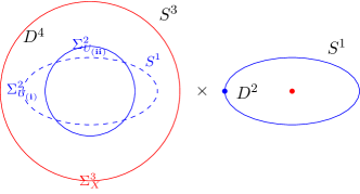
Figure 2: $S^{5}=\partial D^{6}=\partial(D^{4}\times D^{2})=S^{3}\times D^{2}\cup D^{4}\times S^{1}=S^{3}\times D^{2}\cup D^{2}\times D^{2}\times S^{1}$, the intersection of the two copies of $D^{2}\times S^{1}$ in the second piece ($D^{2}\times 0_{\text{pt}}\times S^{1}$ and $0_{\text{pt}}\times D^{2}\times S^{1}$) is $0_{\text{pt}}\times 0_{\text{pt}}\times S^{1}=0_{\text{pt}}\times S^{1}$, this $0_{\text{pt}}\times S^{1}$ and $S^{3}\times 0_{\text{pt}}$ in the first piece are linked. In this figure, $\Sigma^{3}_{X}=S^{3}\times 0_{\text{pt}}$, $\Sigma^{2}_{U_{\bf(i)}}=\partial(D^{2}\times 0_{\text{pt}}\times S^{1})$, $\Sigma^{2}_{U_{\bf(ii)}}=\partial(0_{\text{pt}}\times D^{2}\times S^{1})$.

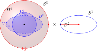
Figure 3: Following the last Fig. 2, $V^{4}_{X}=D^{4}\times 0_{\rm pt}$ which bounds $\Sigma^{3}_{X}$, $V^{3}_{U_{\bf(i)}}=D^{2}\times 0_{\text{pt}}\times S^{1}$ which bounds $\Sigma^{2}_{U_{\bf(i)}}$, $V^{3}_{U_{\bf(ii)}}=0_{\text{pt}}\times D^{2}\times S^{1}$ which bounds $\Sigma^{2}_{U_{\bf(ii)}}$. The intersection of $V^{3}_{U_{\bf(i)}}$ and $V^{3}_{U_{\bf(ii)}}$ is $0_{\text{pt}}\times S^{1}$, the intersection of $V^{4}_{X}$ and this $0_{\text{pt}}\times S^{1}$ is a point which is the point in black in this figure.

To explain, we start by constructing the 5-sphere via $S^{5}=\partial D^{6}=\partial(D^{4}\times D^{2})=S^{3}\times D^{2}\cup D^{4}\times S^{1}=S^{3}\times D^{2}\cup D^{2}\times D^{2}\times S^{1}$. More explicitly, we color the different components as $S^{5}=({\color[rgb]{1,0,0}S^{3}_{\rm L}\times D^{2}_{\rm R}})\cup({\color[rgb]{0,0,1}D^{4}_{\rm L}\times S^{1}_{\rm R}})$ and $S^{5}=({\color[rgb]{1,0,0}S^{3}_{\rm L}\times D^{2}_{\rm R}})\cup({\color[rgb]{0,0,1}D^{2}_{\rm L}\times D^{2}_{\rm L}\times S^{1}_{\rm R}})$.

Consider the link invariant defined by ${\#(V^{4}_{X}\cap V^{3}_{U_{\bf(i)}}\cap V^{3}_{U_{\bf(ii)}})\equiv\text{Tlk}^{(5)}_{w_{1}BB}(\Sigma^{3}_{X},\Sigma^{2}_{U_{\bf(i)}},\Sigma^{2}_{U_{\bf(ii)}})}$, we see that the link configuration in Fig. 2 gives the intersection number 1 in Fig. 3. Again in Fig. 3 associated with the intersection number ${\#(V^{4}_{X}\cap V^{3}_{U_{\bf(i)}}\cap V^{3}_{U_{\bf(ii)}})}$, $(0_{\rm pt-})$ means the point $(0_{\rm pt})$ now is attached to a line. We see the intersection number ${\#(V^{4}_{X}\cap V^{3}_{U_{\bf(i)}}\cap V^{3}_{U_{\bf(ii)}})}=1$ precisely corresponds to the black dot $\bullet$.

6.3 The 2nd Triple Link ${\#(V^{4}_{X_{\bf(i)}}\cap V^{4}_{X_{\bf(ii)}}\cap\Sigma^{2}_{U})\equiv\text{Tlk}^{(5)}_{w_{1}w_{1}\hskip 1.0pt\mathrm{d}B}(\Sigma^{3}_{X_{\bf(i)}},\Sigma^{3}_{X_{\bf(ii)}},\Sigma^{2}_{U})}$ Configuration in 5d

We now discuss $\text{Tlk}^{(5)}_{w_{1}w_{1}\hskip 1.0pt\mathrm{d}B}(\Sigma^{3}_{X_{\bf(i)}},\Sigma^{3}_{X_{\bf(ii)}},\Sigma^{2}_{U})$, or schematically $\text{Tlk}^{(5)}_{AA\hskip 1.0pt\mathrm{d}B}(\Sigma^{3}_{X_{\bf(i)}},\Sigma^{3}_{X_{\bf(ii)}},\Sigma^{2}_{U})$. This link invariant is derived in Sec. 5.2.2.

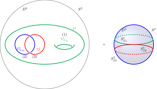
Figure 4: $S^{5}=\partial D^{6}=\partial(D^{3}\times D^{3})=S^{2}\times D^{3}\cup D^{3}\times S^{2}$. Put a 2-torus (denoted by (1)) in $D^{3}\times 0_{\text{pt}}$, and put a Hopf link (the two circles are denoted by (2) and (3) respectively) in the solid 2-torus. Put two circles (denoted by $S^{1}_{(1)}$ and $S^{1}_{(3)}$ respectively) which intersect in only one point in $0_{\text{pt}}\times S^{2}$ (denoted by $S^{2}_{(2)}$). In this figure, $\Sigma^{3}_{X_{\bf(i)}}$ is the cartesian product of the 2-torus (1) and $S^{1}_{(1)}$, $\Sigma^{3}_{X_{\bf(ii)}}$ is the cartesian product of the circle (2) and $S^{2}_{(2)}$, $\Sigma^{2}_{U}$ is the cartesian product of the circle (3) and $S^{1}_{(3)}$.

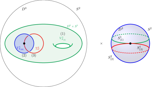
Figure 5: Following the last Fig. 4, if we fill in $\Sigma^{3}_{X_{\bf(i)}}$ and $\Sigma^{3}_{X_{\bf(ii)}}$, we get $V^{4}_{X_{\bf(i)}}=D^{2}\times S^{1}\times S^{1}$ and $V^{4}_{X_{\bf(ii)}}=D^{2}\times S^{2}$, $V^{4}_{X_{\bf(i)}}$, $V^{4}_{X_{\bf(ii)}}$ and $\Sigma^{2}_{U}$ will intersect in only one point which is the point in black in this figure.

Let us consider the link invariant defined by ${{\#(V^{4}_{X_{\bf(i)}}\cap V^{4}_{X_{\bf(ii)}}\cap\Sigma^{2}_{U})\equiv\text{Tlk}^{(5)}_{w_{1}w_{1}\hskip 1.0pt\mathrm{d}B}(\Sigma^{3}_{X_{\bf(i)}},\Sigma^{3}_{X_{\bf(ii)}},\Sigma^{2}_{U})}}$. We see that the link configuration in Fig. 4 gives the intersection number 1 in Fig. 5.

6.4 Quadruple Link
${\#(V^{4}_{X_{\bf(i)}}\cap V^{4}_{X_{\bf(ii)}}\cap V^{4}_{X_{\bf(iii)}}\cap V^{3}_{U})\equiv\text{Qlk}^{(5)}_{w_{1}w_{1}w_{1}B}(\Sigma^{3}_{X_{\bf(i)}},\Sigma^{3}_{X_{\bf(ii)}},\Sigma^{3}_{X_{\bf(iii)}},\Sigma^{2}_{U})}$ Configuration in 5d

We now discuss $\text{Qlk}^{(5)}_{w_{1}w_{1}w_{1}B}(\Sigma^{3}_{X_{\bf(i)}},\Sigma^{3}_{X_{\bf(ii)}},\Sigma^{3}_{X_{\bf(iii)}})$, or schematically $\text{Qlk}^{(5)}_{aaab}(\Sigma^{3}_{X_{\bf(i)}},\Sigma^{3}_{X_{\bf(ii)}},\Sigma^{3}_{X_{\bf(iii)}})$. This link invariant is derived in Sec. 5.2.1.

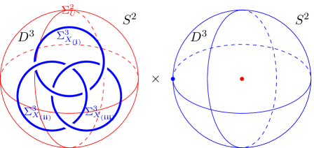
Figure 6: $S^{5}=\partial D^{6}=\partial(D^{3}\times D^{3})=S^{2}\times D^{3}\cup D^{3}\times S^{2}$. Put Borromean rings in $D^{3}\times 0_{\text{pt}}$, If we fill in each of the three circles of the Borromean rings, then we get an intersection point, we can think of this point as $0_{\text{pt}}$ in $D^{3}$, then the cartesian product of each of the three circles and $S^{2}$ (denoted by $\Sigma^{3}_{X_{\bf(i)}}$, $\Sigma^{3}_{X_{\bf(ii)}}$ and $\Sigma^{3}_{X_{\bf(iii)}}$ respectively) will intersect in $0_{\text{pt}}\times S^{2}$, this $0_{\text{pt}}\times S^{2}$ and $S^{2}\times 0_{\text{pt}}$ ($\Sigma^{2}_{U}$ in this figure) are linked.

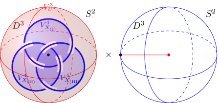
Figure 7: Following the last Fig. 6, we denote the three $D^{2}\times S^{2}$ which bound the cartesian product of the three circles and $S^{2}$ as $V^{4}_{X_{\bf(i)}}$, $V^{4}_{X_{\bf(ii)}}$, $V^{4}_{X_{\bf(iii)}}$ respectively. The intersection of $V^{4}_{X_{\bf(i)}}$, $V^{4}_{X_{\bf(ii)}}$ and $V^{4}_{X_{\bf(iii)}}$ is $0_{\text{pt}}\times S^{2}$. The intersection of $V^{3}_{U}=D^{3}\times 0_{\text{pt}}$ which bounds $\Sigma^{2}_{U}$ and $0_{\text{pt}}\times S^{2}$ is a point which is the point in black in this figure.

Let us consider the link invariant defined by

$${\#(V^{4}_{X_{\bf(i)}}\cap V^{4}_{X_{\bf(ii)}}\cap V^{4}_{X_{\bf(iii)}}\cap V^{3}_{U})\equiv\text{Qlk}^{(5)}_{w_{1}w_{1}w_{1}B}(\Sigma^{3}_{X_{\bf(i)}},\Sigma^{3}_{X_{\bf(ii)}},\Sigma^{3}_{X_{\bf(iii)}},\Sigma^{2}_{U})}$$

. We see that the link configuration in Fig. 6 gives the intersection number 1 in Fig. 7.

6.5 Quadratic Link $\#(V^{3}_{U_{\bf(i)}}\cap\Sigma^{2}_{U_{\bf(ii)}})\equiv\text{Lk}^{(5)}_{B\hskip 1.0pt\mathrm{d}B}(\Sigma^{2}_{U_{\bf(i)}},\Sigma^{2}_{U_{\bf(ii)}})$

Now we discuss $\text{Lk}^{(5)}_{B\hskip 1.0pt\mathrm{d}B}(\Sigma^{2}_{U_{\bf(i)}},\Sigma^{2}_{U_{\bf(ii)}})$. This link invariant is derived in Sec. 5.4.

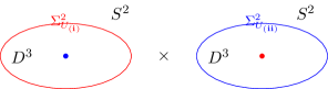
Figure 8: $S^{5}=\partial D^{6}=\partial(D^{3}\times D^{3})=S^{2}\times D^{3}\cup D^{3}\times S^{2}$. The $S^{2}\times 0_{\text{pt}}$ in the first piece and the $0_{\text{pt}}\times S^{2}$ in the second piece are linked. In this figure, $\Sigma^{2}_{U_{\bf(i)}}=S^{2}\times 0_{\text{pt}}$, $\Sigma^{2}_{U_{\bf(ii)}}=0_{\text{pt}}\times S^{2}$.

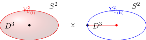
Figure 9: Following the last Fig. 8, if we fill in $S^{2}\times 0_{\text{pt}}$, we get $V^{3}_{U_{\bf(i)}}=D^{3}\times 0_{\text{pt}}$, the intersection of $D^{3}\times 0_{\text{pt}}$ and $0_{\text{pt}}\times S^{2}$ is a point which is the point in black in this figure.

Let us consider the link invariant defined by

$${\#(V^{4}_{X_{\bf(i)}}\cap V^{4}_{X_{\bf(ii)}}\cap V^{4}_{X_{\bf(iii)}}\cap V^{3}_{U})\equiv\text{Qlk}^{(5)}_{w_{1}w_{1}w_{1}B}(\Sigma^{3}_{X_{\bf(i)}},\Sigma^{3}_{X_{\bf(ii)}},\Sigma^{3}_{X_{\bf(iii)}},\Sigma^{2}_{U})}$$

. We see that the link configuration in Fig. 8 gives the intersection number 1 in Fig. 9.

6.6 Quadratic Link $\#(V^{3}_{U^{\prime}}\cap\Sigma^{2}_{U})\equiv\text{Lk}^{(5)}_{w_{2}\hskip 1.0pt\mathrm{d}B}(\Sigma^{2}_{U},\Sigma^{2}_{U^{\prime}})$

Now we discuss $\text{Lk}^{(5)}_{w_{2}\hskip 1.0pt\mathrm{d}B}(\Sigma^{2}_{U^{\prime}},\Sigma^{2}_{U})$ or $\text{Lk}^{(5)}_{B^{\prime}\hskip 1.0pt\mathrm{d}B}(\Sigma^{2}_{U^{\prime}},\Sigma^{2}_{U})$. This link invariant is derived in Sec. 5.3.

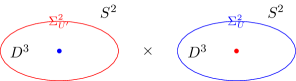
Figure 10: $S^{5}=\partial D^{6}=\partial(D^{3}\times D^{3})=S^{2}\times D^{3}\cup D^{3}\times S^{2}$. The $S^{2}\times 0_{\text{pt}}$ in the first piece and the $0_{\text{pt}}\times S^{2}$ in the second piece are linked. In this figure, $\Sigma^{2}_{U^{\prime}}=S^{2}\times 0_{\text{pt}}$, $\Sigma^{2}_{U}=0_{\text{pt}}\times S^{2}$.

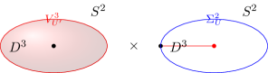
Figure 11: Following the last Fig. 10, if we fill in $S^{2}\times 0_{\text{pt}}$, we get $V^{3}_{U^{\prime}}=D^{3}\times 0_{\text{pt}}$, the intersection of $D^{3}\times 0_{\text{pt}}$ and $0_{\text{pt}}\times S^{2}$ is a point which is the point in black in this figure.

Let us consider the link invariant defined by $\#(V^{3}_{U^{\prime}}\cap\Sigma^{2}_{U})\equiv\text{Lk}^{(5)}_{w_{2}\hskip 1.0pt\mathrm{d}B}(\Sigma^{2}_{U},\Sigma^{2}_{U^{\prime}})$. We see that the link configuration in Fig. 10 gives the intersection number 1 in Fig. 11.

6.7 The 3rd Triple Link ${\#(V^{4}_{X_{\bf(i)}}\cap\Sigma^{3}_{X_{\bf(ii)}}\cap V^{3}_{U})\equiv\text{Tlk}^{(5)}_{(A\hskip 1.0pt\mathrm{d}A)B}(\Sigma^{3}_{X_{\bf(i)}},\Sigma^{3}_{X_{\bf(ii)}},\Sigma^{2}_{U})}$ Configuration in 5d

Finally, we discuss a third triple link invariant ${\#(V^{4}_{X_{\bf(i)}}\cap\Sigma^{3}_{X_{\bf(ii)}}\cap V^{3}_{U})\equiv\text{Tlk}^{(5)}_{(A\hskip 1.0pt\mathrm{d}A)B}(\Sigma^{3}_{X_{\bf(i)}},\Sigma^{3}_{X_{\bf(ii)}},\Sigma^{2}_{U})}$. We have not derived these from 4d YM-5d SET coupled systems. However, to get this, we need a topological term $(w_{1}(TM)\hskip 1.0pt\mathrm{d}w_{1}(TM))B$. This is possible however from $(A_{I}\hskip 1.0pt\mathrm{d}A_{J})B$ type of TQFTs.

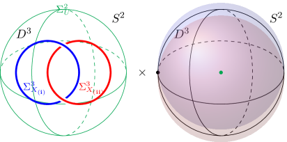
Figure 12: $S^{5}=\partial D^{6}=\partial(D^{3}\times D^{3})=S^{2}\times D^{3}\cup D^{3}\times S^{2}$, put a Hopf link in $D^{3}\times 0_{\rm pt}$. In this figure, $\Sigma^{3}_{X_{\bf(i)}}$ and $\Sigma^{3}_{X_{\bf(i)}}$ are the cartesian product of the two circles in the Hopf link and $S^{2}$ respectively, namely, they are both $S^{1}\times S^{2}$, $\Sigma^{2}_{U}=S^{2}\times 0_{\rm pt}$.

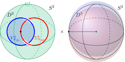
Figure 13: Following the last Fig. 12, if we fill in $\Sigma^{3}_{X_{\bf(i)}}$, we get $V^{4}_{X_{\bf(i)}}=D^{2}\times S^{2}$, the intersection of $V^{4}_{X_{\bf(i)}}$ and $\Sigma^{3}_{X_{\bf(ii)}}$ is the cartesian product of a point (we can think of the point as $0_{\rm pt}$) and $S^{2}$. If we fill in $\Sigma^{2}_{U}$ further, we get $V^{3}_{U}=D^{3}\times 0_{\rm pt}$, the intersection of $D^{3}\times 0_{\rm pt}$ and $0_{\rm pt}\times S^{2}$ is a point which is the point in black in this figure.

Let us consider the link invariant defined by ${\#(V^{4}_{X_{\bf(i)}}\cap\Sigma^{3}_{X_{\bf(ii)}}\cap V^{3}_{U})\equiv\text{Tlk}^{(5)}_{(A\hskip 1.0pt\mathrm{d}A)B}(\Sigma^{3}_{X_{\bf(i)}},\Sigma^{3}_{X_{\bf(ii)}},\Sigma^{2}_{U})}$. We see that the link configuration in Fig. 12 gives the intersection number 1 in Fig. 13.

7 4d SO(3)_θ=π Yang-Mills Gauge Theories coupled to the Boundary of 5d SETs/Long-Range Entangled TQFTs

In Sec. 2, we have shown that that the ${\rm SU}(2)$ Yang-Mills theory with $\theta=\pi$, with the gauge bundle constraint $w_{2}(V_{{\rm PSU}(2)})=B+K_{1}w_{1}(TM)^{2}+K_{2}w_{2}(TM)$, has two distinct ’t Hooft anomalies as shown in Eq. (2.47). In this section, we further comment on gauging the 1-form $\mathbb{Z}_{2,[1]}^{e}$ center symmetry of the Four Siblings of ${\rm SU}(2)_{\theta=\pi}$ YM to obtain ${\rm SO}(3)_{\theta=\pi}$ YM theories. Since the ’t Hooft anomalies involve the 1-form center symmetry and the spacetime symmetries (whose background fields are the Stiefel-Whitney classes $w_{i}(TM)$), depending on which manifold we formulate the ${\rm SU}(2)$ Yang-Mills, one obtains different theories.

7.1 From SU(2) to SO(3) Gauge Theory

To illustrate, we start by gauging the 1-form symmetry [6, 77] of the ${\rm SU}(2)_{\theta=0}$ YM theories which is time-reversal symmetric and anomaly free. There are still four choices of gauge bundle constraints labeled by $(K_{1},K_{2})$, i.e. Eq. (3.1). Let ${\mathbf{Z}}^{\text{$4$d}}_{{{\rm SU}(2)}{\text{YM}}}[B]$ be the path integral without specifying the gauge bundle constraint, the partition function with the gauge bundle constraint $w_{2}(E)=(B+K_{1}w_{1}(TM)^{2}+K_{2}w_{2}(TM))\mod 2$ is

$${\mathbf{Z}}^{\text{$4$d}}_{{{\rm SU}(2)}{\text{YM}}_{(K_{1},K_{2})}}[B]\equiv\int[D\Lambda]\;{\mathbf{Z}}^{\text{$4$d}}_{{{\rm SU}(2)}{\text{YM}}}[B]\exp(\hskip 1.0pt\mathrm{i}\hskip 1.0pt\pi\Lambda\cup(w_{2}(E)-(B+K_{1}w_{1}(TM)^{2}+K_{2}w_{2}(TM)))),$$

More generally, we can add the counter term $\frac{p\pi}{2}\mathcal{P}(B)$ labeled by an integer $p$, which modifies the partition function as

$${\mathbf{Z}}^{\text{$4$d}}_{{{\rm SU}(2)}{\text{YM}}_{(K_{1},K_{2})}}[B]\equiv\int[D\Lambda]\;{\mathbf{Z}}^{\text{$4$d}}_{{{\rm SU}(2)}{\text{YM}}}[B]\exp\big{(}\hskip 1.0pt\mathrm{i}\hskip 1.0pt\pi(\Lambda\cup(w_{2}(E)-(B+K_{1}w_{1}(TM)^{2}+K_{2}w_{2}(TM)))+\frac{p}{2}\mathcal{P}(B))\big{)},$$ (7.1)

Below we would like to obtain ${\rm SO}(3)$ YM by gauging 1-form $\mathbb{Z}_{2,[1]}^{e}$ center symmetry. The theta angle of the resulting theory is $2\pi p$. If $w_{2}(TM)$ is nontrivial, the resulting ${\rm SO}(3)$ theory is time-reversal symmetric only when $p\in 2\mathbb{Z}$ and $p\sim p+4$. When $w_{2}(TM)$ is trivial, the resulting ${\rm SO}(3)$ theory is time-reversal symmetric for $p\in\mathbb{Z}$ and $p\sim p+2$. In the following, we always restrict to the time-reversal symmetric case. Gauging 1-form center symmetry amounts to summing over the background gauge field $B$ (promoting $B$ to a dynamical gauge field),

$${\mathbf{Z}}^{\text{$4$d}}_{{{\rm SO}(3)}{\text{YM}}_{(K_{1},K_{2})}}=\\ \int[D\Lambda][DB]\;{\mathbf{Z}}^{\text{$4$d}}_{{{\rm SU}(2)}{\text{YM}}}[B]\exp\big{(}\hskip 1.0pt\mathrm{i}\hskip 1.0pt\pi(\Lambda\cup(w_{2}(E)-(B+K_{1}w_{1}(TM)^{2}+K_{2}w_{2}(TM)))+\frac{p}{2}\mathcal{P}(B))\big{)}.$$ (7.2)

Integrating out $\Lambda$ enforces the relation between SO(3)-gauge bundles and 2-form dynamical gauge field $B$. This outputs the SO(3)-gauge theory ${\mathbf{Z}}^{\text{$4$d}}_{{{\rm SO}(3)}{\text{YM}}_{(K_{1},K_{2})}}$ with $\theta=2\pi p$.

7.2 Gauging 1-form $\mathbb{Z}_{2,[1]}^{e}$-symmetry of ${\rm SU}(2)$ Gauge Theory with $\theta=\pi$

We proceed to discuss gauging the 1-form symmetry of ${\rm SU}(2)$ Yang-Mills with $\theta=\pi$.

If one formulates the ${\rm SU}(2)_{\theta=\pi}$ Yang-Mills on an orientable and spin manifold, i.e., $w_{1}=w_{2}=0$ (hence $w_{3}=0$ as well), for spacetime tangent bundle $TM$, there is the freedom to ignore the time reversal as a symmetry of the theory. The only symmetry of interest is the 1-form symmetry, which does not have anomaly with itself. Hence one can gauge the 1-form symmetry and the resulting theory is ${\rm PSU}(2)={\rm SO}(3)$ Yang-Mills with $\theta=\pi$. Indeed, ${\rm SO}(3)$ Yang-Mills with $\theta=\pi$ does not respect time reversal, which maps $\theta=\pi$ to $\theta=3\pi$ due to the identification $\theta\sim\theta+4\pi$ on a spin manifold.

If one formulates the ${\rm SU}(2)_{\theta=\pi}$ Yang-Mills on an orientable and non-spin manifold, one still has the freedom to ignore the time reversal as a symmetry of the theory. However, in this case, there is a counter term

$$\int_{M^{5}}K_{2}\pi\mathrm{Sq}^{1}(w_{2}(TM)\cup B)$$ (7.3)

which is a WZW-like term of background fields (i.e., probe fields in condensed matter language). Denoting the partition function of the ${\rm SU}(2)_{\theta=\pi}$ Yang-Mills coupled to $B$ as ${\mathbf{Z}}_{{\rm SU}(2)\mathrm{YM}_{(0,K_{2})}}[M^{4},B]$, after promoting $B$ to a dynamical field, the partition function of the entire 4d-5d system is

$${\int[DB]{\mathbf{Z}}_{{\rm SU}(2)\mathrm{YM}_{(0,K_{2})}}[M^{4},B]\exp\Bigg{(}\hskip 1.0pt\mathrm{i}\hskip 1.0pt\pi\int_{M^{5}}K_{2}\pi\mathrm{Sq}^{1}(w_{2}(TM)\cup B)\Bigg{)}.}$$ (7.4)

If $K_{2}=0$, the 4d-5d system reduces to an intrinsic 4d system. Physically, this corresponds to the case where the gauge charge is a boson. It makes sense to gauge the 1-form symmetry which again gives raise to the time-reversal broken ${\rm SO}(3)$ Yang-Mills theory. If $K_{2}=1$, the theory is still an intrinsic 4d system. Physically, this corresponds to the case where the gauge charge is a fermion.

If one formulates the ${\rm SU}(2)$ Yang-Mills on an unorientable manifold, the time-reversal symmetry is built in, so time-reversal symmetry is too late to be abandoned. Promoting $B$ to a dynamical gauge field, the partition function for the entire 4d-5d system is

$${\int[DB]{\mathbf{Z}}_{{\rm SU}(2)\mathrm{YM}_{(K_{1},K_{2})}}[M^{4},B]\exp\Bigg{[}\hskip 1.0pt\mathrm{i}\hskip 1.0pt\pi\int_{M^{5}}\Bigg{(}B\mathrm{Sq}^{1}B+\mathrm{Sq}^{2}\mathrm{Sq}^{1}B+K_{1}w_{1}(TM)^{2}\mathrm{Sq}^{1}B+K_{2}\mathrm{Sq}^{1}(w_{2}(TM)\cup B)\Bigg{)}\Bigg{]}.}$$ (7.5)

Since $M^{5}$ is unorientable, for all four choices of $(K_{1},K_{2})$, the 5d terms do not vanish (because $B\mathrm{Sq}^{1}B+\mathrm{Sq}^{2}\mathrm{Sq}^{1}B$ is always non-vanishing on unorientable manifold). Hence one can only discuss the 4d-5d system rather than discussing the 4d system alone. We summarize all the above cases in Table 10.

$$(w_{1},w_{2})\backslash(K_{1},K_{2})$$

WZW WZW

Table 10: Possibilities of gauging the ${\rm SU}(2)_{\theta=\pi}$ Yang-Mills theory with gauge bundle constraint $(K_{1},K_{2})$ on a manifold with Stiefel-Whitney (SW) class $(w_{1},w_{2})=(w_{1}(TM),w_{2}(TM))$, where 0 and 1 mean trivial or nontrivial SW classes respectively. The $\checkmark$ means that there is a way to make sense of the resulting gauged theory as a purely 4d theory. The theories labeled by $\times$ means that it only makes sense to discuss the combined 4d-5d systems. The WZW (Wess-Zumino-Witten) means the theory is intrinsically 4d, however, there is a Wess-Zumino-Witten-like term of background fields, which involves a 5d integral (but does not depend on the choice of 5d manifold $M^{5}$).

8 Lattice Regularization, UV completion and Symmetric Anomalous TQFT

In this section, we formulate the partition function of the 5d higher-SPT ${\mathbf{Z}}_{\text{SPT}_{(K_{1}=0,K_{2}=0)}}^{5\text{d}}[M^{5};B]$ on a simplicial complex spacetime. This provides a lattice regularization of the 5d SPT. We also provide lattice realization of (i) 4d higher-symmetry-extended boundary theory or (ii) 4d higher-symmetry-enriched anomalous topologically ordered boundary theory. We will generalize the approach in [54] and follow the Section IX of [55]. In condensed matter physics, this (ii) phenomenon is known as the anomalous surface topological order (firstly noticed in [78]) typically for the 2+1D boundary of 3+1D SPTs, see a review [30].

8.1 Lattice Realization of 4d Higher-SPTs and Higher-Gauge TQFT: 4d Simplicial Complex and 3+1D Condensed Matter Realization

We warm up by considering a lattice realization of 4d Higher-SPTs given by a probe-field partition function

$${\mathbf{Z}}_{\text{SPT}}^{4\text{d}}[M^{4};B]=\exp(\hskip 1.0pt\mathrm{i}\hskip 1.0pt\frac{\pi}{2}\int_{M^{4}}{\cal P}(B))=\exp(\hskip 1.0pt\mathrm{i}\hskip 1.0pt\frac{\pi}{2}\int_{M^{4}}B\cup B+B\underset{{\scriptscriptstyle 1}}{\cup}\delta B).$$ (8.1)

The path integral can be regularized on a triangulated 4-manifold $M^{4}$. The building blocks of $M^{4}$ are 4-simplices. Without loss of generality, we consider an arbitrary 4-simplex which we denote as $(01234)$ where each number labels one vertex. See Fig. 14 for a graphical representation of a 4-simplex. We denote $B_{ijk}$ as restricting the 2-cochain $B$ on the 2-simplex $(ijk)$. We label the path integral amplitude on $(01234)$ as $\omega_{4}(01234)$, i.e.,

$$\begin{split}\omega_{4}(01234)&=\exp\Bigg{[}\hskip 1.0pt\mathrm{i}\hskip 1.0pt\frac{\pi}{2}\Bigg{(}B\cup B+B\underset{{\scriptscriptstyle 1}}{\cup}\delta B\Bigg{)}_{01234}\Bigg{]}\\ &=\exp\Bigg{[}\hskip 1.0pt\mathrm{i}\hskip 1.0pt\frac{\pi}{2}\Bigg{(}B_{012}B_{234}+B_{034}(B_{123}-B_{023}+B_{013}-B_{012})+B_{014}(B_{234}-B_{134}+B_{124}-B_{123})\Bigg{)}\Bigg{]}.\\ \end{split}$$ (8.2)

It is straightforward to verify that $\omega_{4}(01234)$ satisfies the cocycle condition:

$$(\delta\omega_{4})(012345)=\frac{\omega_{4}(12345)\cdot\omega_{4}(01345)\cdot\omega_{4}(01235)}{\omega_{4}(02345)\cdot\omega_{4}(01245)\cdot\omega_{4}(01234)}=1.$$ (8.3)

Figure 14: Graphical representation of a 4-simplex $(01234)$.

8.2 Lattice Realization of 5d Higher-SPTs and Higher-Gauge SETs: 5d Simplicial Complex and 4+1D Condensed Matter Realization

The 5d partition function with $(K_{1}=0,K_{2}=0)$ is

$${\mathbf{Z}}_{\text{SPT}_{(K_{1}=0,K_{2}=0)}}^{5\text{d}}[M^{5}]=\exp\Bigg{(}\hskip 1.0pt\mathrm{i}\hskip 1.0pt\pi\int_{M^{5}}B\mathrm{Sq}^{1}B+\mathrm{Sq}^{2}\mathrm{Sq}^{1}B\Bigg{)}.$$ (8.4)

We start by triangulating the 5d closed spacetime manifold (without boundary) into 5-simplicial complex. There are some useful identities:

$$\begin{split}\mathrm{Sq}^{1}B&=B\underset{{\scriptscriptstyle 1}}{\cup}B=\frac{1}{2}\delta B,\\ \mathrm{Sq}^{2}\mathrm{Sq}^{1}B&=(\mathrm{Sq}^{1}B)\underset{{\scriptscriptstyle 1}}{\cup}(\mathrm{Sq}^{1}B)=\frac{1}{4}(\delta B)\underset{{\scriptscriptstyle 1}}{\cup}(\delta B).\end{split}$$ (8.5)

Note that in the second equality of the first line, we have used the cocycle condition that $\delta B=0\mod 2$. One can express the SPT action Eq. (8.4) in terms of the sum of cup-products of $B$ cochains over 5-simplices

$${\mathbf{Z}}_{\text{SPT}_{(K_{1}=0,K_{2}=0)}}^{5\text{d}}[M^{5}]=\exp\Bigg{(}\hskip 1.0pt\mathrm{i}\hskip 1.0pt\frac{\pi}{2}\sum_{M^{5}}B\cup\delta B+\hskip 1.0pt\mathrm{i}\hskip 1.0pt\frac{\pi}{4}\sum_{M^{5}}\delta B\underset{{\scriptscriptstyle 1}}{\cup}\delta B\Bigg{)}.$$ (8.6)

Figure 15: Graphical representation of a 5-simplex $(012345)$.

Without loss of generality, we consider an arbitrary 5-simplex which we denote as $(012345)$ where each number labels one vertex. See Fig. 15 for a graphical representation of a 5-simplex. We will label the path integral amplitude on the simplex $(012345)$ as $\omega_{5}(012345)$, i.e.,

$$\omega_{5}(012345)=\exp\Bigg{[}\hskip 1.0pt\mathrm{i}\hskip 1.0pt\pi\Bigg{(}\frac{1}{2}B\cup\delta B+\frac{1}{4}\delta B\underset{{\scriptscriptstyle 1}}{\cup}\delta B\Bigg{)}_{012345}\Bigg{]}$$ (8.7)

so that the partition function can be simplified as ${\mathbf{Z}}_{\text{SPT}_{(K_{1}=0,K_{2}=0)}}^{5\text{d}}[M^{5}]=\prod_{(ijklmn)\in M^{5}}\omega(ijklmn)$. Using the definition of the cup products on simplices and the identities Eq. (8.5), we have

$$\begin{split}\left(\mathrm{Sq}^{1}B\right)_{0123}&=\frac{1}{2}(B_{123}-B_{023}+B_{013}-B_{012})\\ \left(\mathrm{Sq}^{2}\mathrm{Sq}^{1}B\right)_{012345}&=\frac{1}{4}((\delta B)_{0345}(\delta B)_{0123}+(\delta B)_{0145}(\delta B)_{1234}+(\delta B)_{0125}(\delta B)_{2345}),\\ &=\frac{1}{4}(\left(-B_{045}-B_{034}+B_{035}+B_{345}\right)\left(-B_{023}-B_{012}+B_{013}+B_{123}\right)\\ &~{}~{}~{}+\left(-B_{045}-B_{014}+B_{015}+B_{145}\right)\left(-B_{134}-B_{123}+B_{124}+B_{234}\right)\\ &~{}~{}~{}+\left(-B_{025}-B_{012}+B_{015}+B_{125}\right)\left(-B_{245}-B_{234}+B_{235}+B_{345}\right)).\end{split}$$ (8.8)

Hence the path integral amplitude on the simplex $(012345)$ is

$$\begin{split}\omega_{5}(012345)=&\exp\Bigg{[}\frac{\hskip 1.0pt\mathrm{i}\hskip 1.0pt\pi}{2}B_{012}(-B_{245}-B_{234}+B_{235}+B_{345})\\ &+\frac{\hskip 1.0pt\mathrm{i}\hskip 1.0pt\pi}{4}\left(-B_{045}-B_{034}+B_{035}+B_{345}\right)\left(-B_{023}-B_{012}+B_{013}+B_{123}\right)\\ &+\frac{\hskip 1.0pt\mathrm{i}\hskip 1.0pt\pi}{4}\left(-B_{045}-B_{014}+B_{015}+B_{145}\right)\left(-B_{134}-B_{123}+B_{124}+B_{234}\right)\\ &+\frac{\hskip 1.0pt\mathrm{i}\hskip 1.0pt\pi}{4}\left(-B_{025}-B_{012}+B_{015}+B_{125}\right)\left(-B_{245}-B_{234}+B_{235}+B_{345}\right)\Bigg{]}.\end{split}$$ (8.9)

It is straightforward to verify that $\omega_{5}(012345)$ satisfies the cocycle condition:

$$(\delta\omega_{5})(0123456)=\frac{\omega_{5}(123456)\cdot\omega_{5}(013456)\cdot\omega_{5}(012356)\cdot\omega_{5}(012345)}{\omega_{5}(023456)\cdot\omega_{5}(012456)\cdot\omega_{5}(012346)}=1.$$ (8.10)

We emphasize that $\omega(012345)$ is a cocycle only when $B$ is a cocycle, i.e., $\delta B=0$. If $B$ is a cochain rather than a cocycle, Eq. (8.4) is not a cocycle, hence cannot be a partition function of a topological field theory.

We further comment on the lattice regularization of theory with various choices of $(K_{1},K_{2})$.

1. When $(K_{1},K_{2})=(0,0)$, as we derived above, there is a lattice regularization of the 5d SPT partition function.

2. When $(K_{1},K_{2})=(1,0)$, the path integral amplitude depends on the first Stiefel-Whitney class $w_{1}(TM)$. Using the method of [29], one can write down the simplicial form of $w_{1}(TM)^{2}$ using the twisted cocycle, with the coefficient in $U(1)_{T}$ due to anti-unitary nature of time-reversal symmetry (in the Hamiltonian formalism of [29]). We will not write down the explicit expression for the cocycle.

3. $(K_{1},K_{2})=(0,1),(1,1)$ has the same anomaly polynomial as $(K_{1},K_{2})=(0,0),(1,0)$ respectively.

Other than the treating $B$ as the background gauge field, we can also sum over $B$ to get the the topologically ordered 5d SET ${\mathbf{Z}}_{\text{SET}_{(K_{1},K_{2})}}^{5\text{d}}[M^{5}]$.

Given that the 5d SPT and 5d SET path integral can be regularized on a lattice, following [29], one can write down the quantum wavefunction via the spacetime path integral. It is also possible to construct a lattice quantum Hamiltonian on the 4D space (on a constant time slice), for both SPTs and SETs, similar to the formulations of [79, 29, 80, 81]. For the topologically ordered 5d SET, we implement the method of [80, 81]:

$$\hat{\bf H}=-\sum_{\text{1-link }\ell}\hat{\bf A}_{\ell}-\sum_{\text{3-simplex}}\hat{\bf B}_{\text{3-simplex}}$$ (8.11)

where $\hat{\bf A}_{\ell}$ is an operator acting on the plaquettes (2-simplex) adjacent to the 1-link $\ell$, and $\hat{\bf B}_{\text{3-simplex}}$ is an operator acting on the boundary of a given 3-simplex which again are plaquettes (2-simplex). The $\hat{\bf A}_{\ell}$ has its effect on imposing the time evolution constraint as the same as the path integral formulation: $\hat{\bf A}_{\ell}$ lifting the state vector to a next time slice locally around the 1-link $\ell$. The $\hat{\bf B}_{\text{3-simplex}}$ imposes the zero flux condition enclosed by the 3-simplex (which is a 2-sphere $S^{2}$ in topology). We will not give the explicit expression of the quantum Hamiltonian $\hat{\bf H}$ in this work.

8.3 Higher-Symmetry-Extended 3+1D Gapped Boundaries

One option to saturate the anomaly inflow from the bulk 5d (4+1D) SPT is to extend the global symmetry on the 4d (3+1D) boundary, based on the symmetry-extension method of [54]. Note that $(K_{1},K_{2}=0)$ and $(K_{1},K_{2}=1)$ theories have the same 4d anomaly, they are differed by a 4d WZW-like counter term written on a 5d $M^{5}$,

$${\mathbf{Z}}_{\text{SPT}_{(K_{1},K_{2})}}^{5\text{d}}[M^{5}]={\mathbf{Z}}_{\text{SPT}_{(K_{1},0)}}^{5\text{d}}[M^{5}]\exp\Big{(}{\hskip 1.0pt\mathrm{i}\hskip 1.0pt\pi\int_{M^{5}}K_{2}\mathrm{Sq}^{1}(w_{1}(TM)^{2}B)}\Big{)}.$$

The 4d counter term is shown to be vanished on a closed $M^{5}$ in 5d in Eq. (• ‣ 2). Due to Eq. (• ‣ 2), this $K_{2}$-dependent term has no consequences via any anomaly consideration on 4d dynamics. Thus we only discuss the $3+1$D gapped boundary for the two siblings $(K_{1},K_{2}=0)$. The 5d partition function is

$$\begin{split}{\mathbf{Z}}_{\text{SPT}_{(K_{1},0)}}^{5\text{d}}[M^{5}]&=\exp\Big{(}{\hskip 1.0pt\mathrm{i}\hskip 1.0pt\pi\int_{M^{5}}B\mathrm{Sq}^{1}B+\mathrm{Sq}^{2}\mathrm{Sq}^{1}B+K_{1}w_{1}(TM)^{2}\mathrm{Sq}^{1}B}\Big{)}\\ &=\exp\Big{(}{\hskip 1.0pt\mathrm{i}\hskip 1.0pt\pi\int_{M^{5}}(B+(1+K_{1})w_{1}(TM)^{2}+w_{2}(TM))\cup\mathrm{Sq}^{1}B}\Big{)}\cdot\exp\Big{(}\hskip 1.0pt\mathrm{i}\hskip 1.0pt\pi\int_{M^{5}}\delta(...)\Big{)}.\end{split}$$ (8.12)

In the second line, we have used $\int_{M^{5}}\mathrm{Sq}^{2}\mathrm{Sq}^{1}B=\int_{M^{5}}(w_{1}(TM)^{2}+w_{2}(TM))\mathrm{Sq}^{1}B+\int_{M^{5}}\delta(...)$. Note that when $M^{5}$ is closed, the total derivative vanishes and we have the standard Wu formula $\int_{M^{5}}\mathrm{Sq}^{2}\mathrm{Sq}^{1}B=\int_{M^{5}}(w_{1}(TM)^{2}+w_{2}(TM))\mathrm{Sq}^{1}B$. When $M^{5}$ has a boundary, the standard Wu formula may no longer hold, and they differ at most by a co-boundary term. We denote the co-boundary term as $\delta(...)$ in the second line. Since $(...)$ is a well-defined term of background gauge fields, it is a 4d invertible TQFT, which does not contribute to the 4d dynamics. Hence in the construction of 4d symmetric boundary TQFT below, we only focus on the first part in the second line of Eq. (8.12). Using the systematic way in [54] and its generalized higher-symmetry extension [55], we find that the boundary of 5d SPT can support a 4d TQFT via the higher-symmetry extension from a 1-form $\mathbb{Z}_{2}$ to a 1-form $\mathbb{Z}_{4}$ symmetry. Schematically, let $\omega^{(K_{1},0)}_{5}$ be the 5-cocycle whose product over the 5d manifold $M^{5}$ gives the 5d SPT partition function Eq. (8.12). Let $\beta^{(K_{1},0)}_{4}$ be a 4-cochain which trivializes the 5d cocycle, i.e.,

$$\omega^{(K_{1},0)}_{5}=\delta\beta^{(K_{1},0)}_{4}.$$ (8.13)

We find that the following $\beta^{(K_{1},0)}_{4}$ satisfies Eq. (8.13):

$$\beta^{(K_{1},0)}_{4}=\exp\Bigg{[}\hskip 1.0pt\mathrm{i}\hskip 1.0pt\pi\int_{M^{4}}(B+(1+K_{1})w_{1}(TM)^{2}+w_{2}(TM))\cup\gamma(C)\Bigg{]},$$ (8.14)

where $C$ is a $\mathbb{Z}_{4}$ valued 2-cochain satisfying $B=C\mod 2$, and $\gamma:\mathbb{Z}_{4}\to\mathbb{Z}_{2}$ is a function which maps the $\mathbb{Z}_{4}$ 2-cochain to a $\mathbb{Z}_{2}$ 2-cochain:

$$\left(\gamma(C)\right)_{ijk}=\frac{(C_{ijk})^{2}-C_{ijk}}{2}.$$ (8.15)

In summary, the $\beta^{(K_{1},0)}_{4}$ in (8.14) is the partition function of the higher-symmetry-extended 3+1D gapped boundary, while the original 1-form anomalous global symmetry $\mathbb{Z}_{2,[1]}$ is extended to the anomaly-free 1-form global symmetry $\mathbb{Z}_{4,[1]}$. We can also rephrase that the higher-anomaly associated to the bordism group $\Omega_{5}^{{\rm O}}(\mathrm{B}^{2}\mathbb{Z}_{2})$ with a higher classifying space $\mathrm{B}^{2}\mathbb{Z}_{2}$ can be pulled back and trivialized as fully anomaly-free in the bordism group $\Omega_{5}^{{\rm O}}(\mathrm{B}^{2}\mathbb{Z}_{4})$ with an extended higher classifying space $\mathrm{B}^{2}\mathbb{Z}_{4}$:

$$\begin{array}[]{c}\mathrm{B}^{2}\mathbb{Z}_{2}\\ \text{}\\ \text{}\\ \text{}\end{array}\begin{array}[]{c}\longrightarrow\\ \text{}\\ \text{}\\ \text{}\end{array}\begin{array}[]{c}\mathrm{B}^{2}\mathbb{Z}_{4}\\ \text{(Extended global symmetry }\\ \text{$\mathbb{Z}_{4}$ 1-form symmetry probe}\\ \text{by $\mathbb{Z}_{4}$ 2-cochain $C$ background field)}\end{array}\begin{array}[]{c}\longrightarrow\\ \text{}\\ \text{}\\ \text{}\end{array}\begin{array}[]{c}\mathrm{B}^{2}\mathbb{Z}_{2}\\ \text{(Global Symmetry}\\ \text{$\mathbb{Z}_{2}$ 1-form symmetry probe}\\ \text{by $\mathbb{Z}_{2}$ 2-cochain $B$ background field)}\end{array}.$$ (8.16)

This higher-symmetry-extended 3+1D gapped boundary, described by (8.14), has no long-range entanglement and no intrinsic topological order. This higher-symmetry-extended 3+1D gapped boundary is known as the System (i) in Section 7 of Ref. [13] as a short-range entangled state, both in the bulk and on the boundary (denoted as SRE/SRE in Section 7 of Ref. [13]). In fact, this whole SRE/SRE bulk-boundary theory is still an invertible TQFT with a partition function $|{\mathbf{Z}}|=1$ on an $M^{5}$ with a 4d gapped boundary $M^{4}$.

8.4 Higher-Symmetry Anomalous 3+1D Topologically Ordered Gapped Boundaries: Spontaneous Higher-Symmetry Breaking

There also exists another boundary theory of the 5d SPTs in Eq. (8.12), with $\mathbb{Z}_{2}$ 2-cochain $b$ summed over as dynamical fields on the boundary. The boundary theory is a dynamical $\mathbb{Z}_{2}$ gauge theory, which can be obtained from gauging the normal $\mathbb{Z}_{2,[1]}$ subgroup of $\mathbb{Z}_{4,[1]}$ in the symmetry extended gapped boundary from the previous section. Schematically, we promote the 2-form (or 2-cochain) gauge field $b$ coupling to 1-form $\mathbb{Z}_{2,[1]}$-symmetry to dynamical, in a normal subgroup of $\mathbb{Z}_{4,[1]}$. The resulting boundary theory has long range entanglement in contrast to the short range entanglement of the symmetric extended boundary theory in the previous section Sec. 8.3. This can be summarized as an induced fiber sequence of their higher classifying space $\mathrm{B}^{2}\mathbb{Z}_{2}\to\mathrm{B}^{2}\mathbb{Z}_{4}\to\mathrm{B}^{2}\mathbb{Z}_{2}$:

$$\begin{array}[]{c}\mathrm{B}^{2}\mathbb{Z}_{2}\\ \text{(Dynamical/emergent}\\ \text{gaugeable}\\ \text{$\mathbb{Z}_{2}$ 2-cochain $b$ field)}\end{array}\begin{array}[]{c}\longrightarrow\\ \text{}\\ \text{}\\ \text{}\end{array}\begin{array}[]{c}\mathrm{B}^{2}\mathbb{Z}_{4}\\ \text{}\\ \text{}\\ \text{}\end{array}\begin{array}[]{c}\longrightarrow\\ \text{}\\ \text{}\\ \text{}\end{array}\begin{array}[]{c}\mathrm{B}^{2}\mathbb{Z}_{2}\\ \text{(Global Symmetry}\\ \text{$\mathbb{Z}_{2,[1]}$ symmetry probed by}\\ \text{$\mathbb{Z}_{2}$ 2-cochain background $B$ field)}\end{array}.$$ (8.17)

Or we may denote the above as $\mathrm{B}^{2}\mathbb{Z}_{2}^{\text{gauged}}\to\mathrm{B}^{2}\mathbb{Z}_{4}^{\text{total}}\to\mathrm{B}^{2}\mathbb{Z}_{2}^{G}$, implementing the notations of [54, 13].

However, as noticed in Ref. [54] and in section 7 of Ref. [13], when the boundary theory is long-range entangled (after gauging a normal subgroup), it is possible that the new fate of low energy dynamics may not preserve the global symmetry. Specifically, Ref. [54] finds that, under the exact sequence $K\to H\to G$, even for a successful $H$-symmetry extended construction of gapped boundary, in certain cases, dynamically gauging the normal subgroup $K$ may still result in $G$ spontaneously broken. In short, we should question:

Is it possible that $\mathbb{Z}_{2,[1]}$ global symmetry in the long-range entangled boundary theory happens to be spontaneously broken?

Namely, following the notations in Sec. 7 of Ref. [13] on the bulk/boundary (denoted bulk/bdry) systems of the SRE/SRE and SRE/LRE types, the symmetry-extension construction [54, 13] under the exact sequence $K\to H\to G$, may result in different dynamical fates:

$$\left\{\begin{array}[]{l}\text{\emph{Case 1. $H$-symmetry-extended gapped boundary: SRE bulk/SRE bdry.}}\\ \text{e.g. The 1-form $\mathbb{Z}_{4,[1]}$-symmetry extended in Sec.~{}\ref{sec:higher-sym-extended-3+1D}. Many 0-form $G$-symmetry examples given in Ref.~{}\cite[cite]{[\@@bibref{}{Wang2017locWWW1705.06728}{}{}]}}\\[5.69054pt] \text{\emph{Case 2. $G$-symmetry-preserving anomalous $K$-gauge gapped boundary: SRE bulk/LRE bdry.}}\\ \text{e.g. Many 0-form $G$-symmetry examples given in Ref.~{}\cite[cite]{[\@@bibref{}{Wang2017locWWW1705.06728}{}{}]}}.\\[5.69054pt] \text{\emph{Case 3. $G$-symmetry-breaking $K$-gauge gapped boundary: SRE bulk/LRE bdry.}}\\ \text{e.g. Ref.~{}\cite[cite]{[\@@bibref{}{Wang2017locWWW1705.06728}{}{}]}'s Sec.~{}3.4 and Appendix A.2.4, and Ref.~{}\cite[cite]{[\@@bibref{}{Wang2018edf1801.05416}{}{}]}'s Sec.~{}7.1.}\end{array}.\right.$$

Thus below what we aim to examine is whether a proposal of Case 2 associated with Eq. (8.17) is in fact the Case 3 in disguise, when $K$ is dynamically gauged, as

$$\begin{array}[]{c}\mathrm{B}^{2}\mathbb{Z}_{2}\\ \text{(Dynamical/emergent}\\ \text{gaugeable}\\ \text{$\mathbb{Z}_{2}$ 2-cochain $b$ field)}\end{array}\begin{array}[]{c}\longrightarrow\\ \text{}\\ \text{}\\ \text{}\end{array}\begin{array}[]{c}\mathrm{B}^{2}\mathbb{Z}_{4}\\ \text{}\\ \text{}\\ \text{}\end{array}\begin{array}[]{c}\longrightarrow\\ \text{}\\ \text{}\\ \text{}\end{array}\begin{array}[]{c}\mathrm{B}^{2}\mathbb{Z}_{2}\\ \text{(Global Symmetry}\\ \text{$\mathbb{Z}_{2,[1]}$ symmetry}\\ \text{spontaneously broken?)}\end{array}.$$ (8.18)

Concretely, we propose a $\mathbb{Z}_{2}$ gauge theory (endorsed with a $\mathbb{Z}_{2}$ 2-cochain $b$ field and the dual $\mathbb{Z}_{2}$ 1-cochain ${\tilde{a}}$ field, as a candidate IR theory of the UV SU(2) YM) which has $\mathbb{Z}_{2,[1]}$ global symmetry and saturates the ’t Hooft anomaly Eq. (8.12). We will find that the $\mathbb{Z}_{2,[1]}$ global symmetry is spontaneously broken.

We consider the 4d $\mathbb{Z}_{2}$-gauge TQFT

$$\int[Db][D{\tilde{a}}]\exp(\hskip 1.0pt\mathrm{i}\hskip 1.0pt\pi\int_{M^{4}}b\delta{\tilde{a}}+\frac{1}{4}{\cal P}(\delta{\tilde{a}}))=\int[Db][D{\tilde{a}}]\exp(\hskip 1.0pt\mathrm{i}\hskip 1.0pt\pi\int_{M^{4}}b\delta{\tilde{a}}+{\tilde{a}}{\tilde{a}}{\tilde{a}}{\tilde{a}}).$$ (8.19)

Here $\int[Db][D{\tilde{a}}]$ means we sum over the $\mathbb{Z}_{2}$ valued 2-cochain $b\in C^{2}(M,\mathbb{Z}_{2})$ and $\mathbb{Z}_{2}$ valued 1-cochain ${\tilde{a}}\in C^{1}(M,\mathbb{Z}_{2})$. The first term is the standard BF term of discrete gauge theory, while the second term is the 4d analogue of the Dijkgraaf-Witten type action[12]. We also refer it as the twisting term. Integrating out $b$ enforces ${\tilde{a}}$ to be a $\mathbb{Z}_{2}$ valued cocycle, hence the twisting term $\frac{1}{4}{\cal P}(\delta{\tilde{a}})=\frac{1}{4}\delta{\tilde{a}}\delta{\tilde{a}}={\tilde{a}}{\tilde{a}}{\tilde{a}}{\tilde{a}}$ mod 2 is time-reversal symmetric. To match the anomaly from 5d SPTs in Eq. (8.12), we couple to background fields $B$ and $w_{1}(TM)$, as follows,

$$\pi\int_{M^{4}}b(\delta{\tilde{a}}-B-K_{1}w_{1}(TM)^{2})+\frac{1}{4}{\cal P}(\delta{\tilde{a}}-B)$$ (8.20)

Summing over the $\mathbb{Z}_{2}$ valued 2-cochain $b$ enforces the gauge bundle constraint:

$$\delta{\tilde{a}}=B+K_{1}w_{1}(TM)^{2}\mod 2.$$ (8.21)

Notice that under the gauge transformation of the background field $B\to B+\delta\lambda$, we demand $\tilde{a}\to\tilde{a}+\lambda$. It is obvioius that the action Eq. (8.20) is gauge invariant. However, due to the gauge bundle constraint Eq. (8.21), the twisting term $\frac{\pi}{4}{\cal P}(\delta\tilde{a}-B)$ is no longer $0$ or $\pi\mod 2\pi$, hence it is not time-reversal invariant, and Eq. (8.20) is not well defined on an unorientable manifold. To make sense of the theory on an unorientable manifold, we use the same idea in Sec. 2 where we promote the twisting term to a 5d integral,

$$\begin{split}\pi\int_{M^{5}}\frac{1}{4}\delta{\cal P}(\delta{\tilde{a}}-B)&=\pi\int_{M^{5}}\frac{1}{2}\delta\tilde{a}\delta(\delta\tilde{a})+\frac{1}{2}\delta B\delta\tilde{a}+\frac{1}{4}\delta{\cal P}(B)\\ &=\pi\int_{M^{5}}B\mathrm{Sq}^{1}B+\mathrm{Sq}^{2}\mathrm{Sq}^{1}B+K_{1}w_{1}(TM)^{2}\mathrm{Sq}^{1}B\end{split}$$ (8.22)

where we have used $\frac{\pi}{4}\delta{\cal P}(B)=\pi(B\mathrm{Sq}^{1}B+\mathrm{Sq}^{2}\mathrm{Sq}^{1}B)$ and the gauge bundle constraint Eq. (8.21). Thus when we couple theory to the background field $B$ and formulate it on an unorientable manifold, only the 4d-5d coupled system is well defined

$$\int[Db][D{\tilde{a}}]\exp\big{(}\hskip 1.0pt\mathrm{i}\hskip 1.0pt\pi\int_{M^{4}}b(\delta{\tilde{a}}-B-K_{1}w_{1}(TM)^{2})+\hskip 1.0pt\mathrm{i}\hskip 1.0pt\pi\int_{M^{5}}(B\mathrm{Sq}^{1}B+\mathrm{Sq}^{2}\mathrm{Sq}^{1}B+K_{1}w_{1}(TM)^{2}\mathrm{Sq}^{1}B)\big{)}.$$ (8.23)

Indeed, the 5d integral implies that the $\mathbb{Z}_{2}$ gauge theory saturates the anomaly Eq. (8.12). Let us comment on the dynamics of the above 4d $\mathbb{Z}_{2}$ gauge theory. The fact that $\tilde{a}$ transforms as $\tilde{a}\to\tilde{a}+\lambda$ under 1-form background gauge transformation $B\to B+\delta\lambda$ suggests that the Wilson line

$$\exp(\hskip 1.0pt\mathrm{i}\hskip 1.0pt\pi\oint{\tilde{a}})$$ (8.24)

has a charge 1 under $\mathbb{Z}_{2,[1]}$. In a TQFT, any genuine line operators are tensionless, thus the expectation does not satisfy area law. Since $\exp(\hskip 1.0pt\mathrm{i}\hskip 1.0pt\pi\oint{\tilde{a}})$ is a genuine line operator, it obeys a perimeter law, and it spontaneously breaks the $\mathbb{Z}_{2,[1]}$ 1-form symmetry.

We comment that in Section 7.1 of Ref. [13], similar arguments have been used to show that the 0-form $\mathbb{Z}_{2}$ global symmetry of a 2d TQFT is spontaneously broken. In its 2d action $\pi\int\alpha(\delta\phi-A)+\dots$, there is a scalar $\phi$ with charge 1 under $\mathbb{Z}_{2}$ 0-form global symmetry whose background field is $A$. (The $\phi$ and $\alpha$ are dynamical 0-cochain and 1-cochain fields.) In the 2d TQFT, $\phi$ has a nontrivial expectational value $\langle\phi\rangle\neq 0$. Thus the $\mathbb{Z}_{2}$ 0-form symmetry is spontaneously broken. See Ref. [13] for more details.

The fact that the dynamical $\mathbb{Z}_{2}$ gauge theory we constructed spontaneously breaks the 1-form $\mathbb{Z}_{2,[1]}$-symmetry is consistent with the conclusion pointed out by Cordova and Ohmori (see [83] and [84]) where the authors showed the impossibility of having any $\mathbb{Z}_{2}^{T}\times\mathbb{Z}_{2,[1]}$ symmetric anomalous gapped 4d TQFT saturating the 4d higher-anomaly of 5d SPTs Eq. (8.12).

9 Conclusions, Discussions and Dynamics

1. Summary: In this work, we proved (physically via the quantum field theory method) that 4d time-reversal symmetric pure Yang-Mills of an SU(2) gauge group with a second-Chern-class topological term at $\theta=\pi$ (i.e., SU(2)_θ=π YM) have new higher ’t Hooft anomalies in 4d, given by a 5d topological term Eq. (2.47) and Eq. (2.70):

   $${\pi\int_{M^{5}}\Bigg{(}B\cup\mathrm{Sq}^{1}B+\mathrm{Sq}^{2}\mathrm{Sq}^{1}B+K_{1}w_{1}(TM)^{2}\cup\mathrm{Sq}^{1}B+K_{2}\mathrm{Sq}^{1}(w_{2}(TM)\cup B)\Bigg{)}}.$$

   The 5d term $B\mathrm{Sq}^{1}B+\mathrm{Sq}^{2}\mathrm{Sq}^{1}B+K_{1}w_{1}(TM)^{2}\mathrm{Sq}^{1}B$ is a 5d bordism invariant (or equivalently 5d iTQFT/SPTs/counter term) specifies the 4d ’t Hooft anomaly. However, the 5d term $K_{2}\mathrm{Sq}^{1}(w_{2}(TM)B)$ is not a 5d bordism invariant but only a 4d WZW-like counterterm, thus strictly speaking it does not indicate any 4d ’t Hooft anomaly. We found that there are at least Four Siblings of SU(2)_θ=π YM with bosonic UV completion, labeled by $(K_{1},K_{2})\in(\mathbb{Z}_{2},\mathbb{Z}_{2})$. Their higher ’t Hooft anomalies of generalized global symmetries indicate that 4d SU(2)_θ=π YM, in order to realize all global symmetries locally, necessarily couple to 5d higher symmetry-protected topological states (SPTs, as invertible TQFTs [iTQFTs], as 5d 1-form-center-symmetry-protected interacting “topological superconductors” in condensed matter).

   We explored various 4d YM gauge theories living as boundary conditions of 5d gapped short/long-range entangled (SRE/LRE) topological states. We revisited 4d SU(2)_θ=π YM-5d SRE-higher-SPTs coupled systems [5, 8]. Follow Weyl’s gauge principle, by dynamically gauging the 1-form center symmetry, we transformed a 5d bulk SRE SPTs into an LRE symmetry-enriched topologically ordered state (SETs); thus we obtained the 4d SO(3)_θ=π YM-5d LRE-higher-SETs coupled system with dynamical higher-form gauge fields. We illustrate such 4d-5d systems schematically in Fig. 1 and Fig. 16.

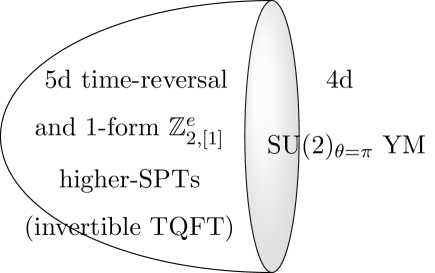
   (a) (b)

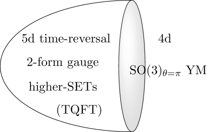
   Figure 16: An alternative illustration of Fig. 1: Various 4d Yang-Mills gauge theories (YM) live as the boundary conditions of certain 5d invertible TQFT (iTQFT) or 5d TQFT, in order to realize YM’s (higher) global symmetries locally.

   The 4d SO(3) YM has a $\theta$ periodicity $\theta\sim\theta+4\pi$ on a spin manifold (due to that the instanton number becomes fractional as half integer $\int_{M^{4}}\frac{1}{8\pi^{2}}\text{Tr}\,(F_{a}\wedge F_{a})\in\frac{1}{2}\mathbb{Z}$), and $\theta\sim\theta+8\pi$ on a non-spin manifold (due to that the instanton number becomes quarter integer as $\int_{M^{4}}\frac{1}{8\pi^{2}}\text{Tr}\,(F_{a}\wedge F_{a})\in\frac{1}{4}\mathbb{Z}$). Since time-reversal symmetry is preserved if and only if $\theta\to-\theta$ is identified, thus SO(3)_θ=π YM explicitly breaks the time-reversal symmetry at ${\theta=\pi}$. In the right-hand side (b) of Fig. 1 and Fig. 16, we actually have a 5d SETs whose 4d boundary explicitly breaks time-reversal symmetry.

   Apply the tool introduced in [12], we derive new exotic anyonic statistics of extended objects such as 2d worldsheet of strings and 3d worldvolume of branes, which physically characterize the 5d SETs. We discover new triple and quadruple link invariants associated with the underlying 5d higher-gauge TQFT, hinting a new intrinsic relation between non-supersymmetric 4d pure YM and topological links in 5d.

2. Appearances of mod 2 anomalies: We note that the anomaly associated to the 5d term $\exp(\hskip 1.0pt\mathrm{i}\hskip 1.0pt\pi\int w_{3}(TM)B)$ has also appeared in the context of an adjoint QCD₄ theory ([85, 86, 87] and [55]). The $\exp(\hskip 1.0pt\mathrm{i}\hskip 1.0pt\pi\int w_{2}(TM)w_{3}(TM))$ has also appeared as a new SU(2) anomaly in the SU(2) gauge theory [57]. All these anomalies and all our anomalies in Eq. (2.70) are mod 2 non-perturbative global anomalies, like the SU(2) anomalies [56, 57].

3. Mathematical relation between 5d and 4d bordism groups: Mathematically there seems to be an amusing relation between (1) gauging the SU(2) gauge bundle/connection under the coupling of 4d YM with 4d SPTs (4d bordism invariants of $\Omega^{G^{\prime}}_{4}$) with $G^{\prime}$ derived from a group extension Eq. (3.2):

   $$1\to{\rm SU}(2)\to G^{\prime}\to{\rm O}(d)\to 1;$$

   and (2) some of the 5d bordism invariants given by ${\Omega_{5}^{{\rm O}}(\mathrm{B}^{2}\mathbb{Z}_{2})=\mathbb{Z}_{2}^{4}}$. We provide the computations of bordism groups and topological invariants in Appendix A. It will be illuminating to explore this relation further in the future.

   

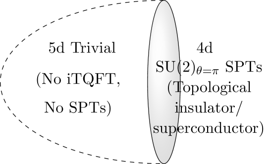
   Figure 17: 4d time-reversal and SU(2) symmetric-protected topological states (SPTs) can be defined as 4d iTQFTs/bordism invariants. Their symmetries can be realized locally in 4d, without the need to an extra dimensional 5d system. Gauging SU(2) symmetry of this 4d SPTs renders the 4d-5d coupled system in Fig. 16(a). Further gauging $\mathbb{Z}_{2,[1]}^{e}$-symmetry of the whole system in Fig. 16(a) renders the 4d-5d coupled system in Fig. 16(b). See the remark 4 of Sec. 9 for details.

4. Classes of 4d SU(2)_θ=π YM: In Ref. [38], it was noted that the Pin⁺ and Pin^- version of the above group extensions $G^{\prime}={\mathrm{Pin}^{+}\times_{\mathbb{Z}_{2}}{\rm SU}(2)}$ and $G^{\prime}={\mathrm{Pin}^{-}\times_{\mathbb{Z}_{2}}{\rm SU}(2)}$ provide two different SPTs vacua after dynamically gauging the SU(2) symmetry give rise to two distinct 4d SU(2)_θ=π YM theories. Although Ref. [38] suggested that the Pin⁺ and Pin^- of 4d SU(2)_θ=π YM are secretly indistinguishable by correlators of local operators on orientable spacetimes nor by gapped SPT states, can be distinguished on non-orientable spacetimes or potentially by correlators of extended operators.

   In this work, we have shown that Pin⁺ and Pin^- of 4d SU(2)_θ=π YM indeed have distinct new higher ’t Hooft anomalies, given by Eq. (2.47) and Eq. (2.70), with $(K_{1},K_{2})=(0,1)$ and $(K_{1},K_{2})=(1,1)$ respectively. Thus we confirm that Pin⁺ and Pin^- of 4d SU(2)_θ=π YM live in distinct Hilbert spaces, thus they are indeed distinct vacua.

   More generally, in this work, we propose a classification 4d SU(2)_θ=π YM with a bosonic UV completion (e.g., on a lattice with bosonic degrees of freedom) and without fermionic parity symmetry $\mathbb{Z}_{2}^{F}$. We propose that a classification can be all obtained from dynamically gauging the SU(2) normal subgroup of 4d $G^{\prime}$-SPTs where $G^{\prime}$ is given by Eq. (3.2): $1\to{\rm SU}(2)\to G^{\prime}\to{\rm O}(d)\to 1,$ i.e., follow [38] by coupling the 4d $G^{\prime}$-SPTS to a pure 4d SU(2) YM theory and dynamically gauge their ${\rm SU}(2)$, see Sec. 3. Other than the Pin⁺ and Pin^- cases, this extension Eq. (3.2) includes two more cases: $G^{\prime}={\rm{O}(d)\times SU(2)}$ and ${\rm{E}(d)\times_{\mathbb{Z}_{2}}SU(2)}$. In summary, in terms of the un-gauged 4d SPTs, we have the symmetry group $G^{\prime}$ [41, 38]:

   $$G^{\prime}=\left\{\begin{array}[]{l}{\rm{O}(d)\times SU(2)}\text{ (bosonic, relates to $(K_{1},K_{2})=(0,0)$)},\\ {\rm{E}(d)\times_{\mathbb{Z}_{2}}SU(2)}\text{ (bosonic, relates to $(K_{1},K_{2})=(1,0)$)},\\ {\mathrm{Pin}^{+}\times_{\mathbb{Z}_{2}^{F}}{\rm SU}(2)}\text{ (fermionic, relates to $(K_{1},K_{2})=(0,1)$)},\\ {\mathrm{Pin}^{-}\times_{\mathbb{Z}_{2}^{F}}{\rm SU}(2)}\text{ (fermionic, relates to $(K_{1},K_{2})=(1,1)$)}.\end{array}\right.$$ (9.1)

   The global symmetries of SPTs for the first two cases are purely bosonic since they do not contain $\mathbb{Z}_{2}^{F}$; the later two cases are fermionic since they do contain $\mathbb{Z}_{2}^{F}$ (the $\mathbb{Z}_{2}^{F}$ is shared by Pin and by the center of SU(2)).

   • Before gauging, see Fig. 17, the 4d SPTs are well-defined 4d topological terms/bordism invariants that can live on 4d with fully local onsite symmetry without the need of an extra 5d bulk.

   • After gauging SU(2) normal subgroup of $G^{\prime}$ symmetry of these SPTs, see Fig. 16(a), there is an emergent 1-form center $\mathbb{Z}_{2,[1]}^{e}$-symmetry. After gauging SU(2), all four systems become bosonic without $\mathbb{Z}_{2}^{F}$ symmetry. We obtain new theories: 4d SU(2)_θ=π YM as boundary conditions of 5d iTQFT in order to realize all global symmetries locally.

   • Furthermore, after gauging this $\mathbb{Z}_{2,[1]}^{e}$-symmetry of the 4d SU(2)_θ=π YM and 5d iTQFT coupled system, see Fig. 16(b), we obtain new theories: 4d SO(3)_θ=π YM as boundary conditions of 5d TQFT.

5. Quantum spin liquids in condensed matter: Strong coupled gauge theories have condensed matter implications as quantum spin liquids. Time-reversal symmetric U(1) gauge theories as quantum spin liquids [30] have been explored and classified based on the quantum numbers of gapped electric and magnetic excitations (Wilson and ’t Hooft line operators) in Ref. [63, 64], see also recent works [88, 89]. Time-reversal symmetric SU(N) gauge theories as quantum spin liquids have been explored in [38]. We will leave additional interpretations of our results of non-abelian SU(2) gauge theories in the context of quantum spin liquids for a future work.

6. Relations of link invariants and braiding statistics in various dimensions: We have applied the tools developed in [12] to compute link invariants of 5d higher-gauge TQFTs in Sec. 4. We anticipate a precise mathematical formulation of this 5d higher-gauge TQFT requires a certain higher category theory. We remark that several link invariants that we find here in 5d have dimensionally reduction analogy to 4d and 3d, such that the dimensional reduced link configurations in 4d and 3d are related to what had been studied in [11], [12] and References therein.

7. Fate of IR dynamics of gauge theories, UV completion and lattice regularizations at $\theta=\pi$: For the 4d-5d systems that we explore (schematically in Fig. 1 and Fig. 16), we mainly focus on their Four Siblings as the UV theories. We do not yet know the IR fate of their dynamics of these strongly coupled gauge theories. However, given the potentially complete ’t Hooft anomalies in Eq. (2.47) and Eq. (2.70) (at zero temperature), we can constrain the IR dynamics by UV-IR anomaly matching.

   The consequence of anomaly matching implies that the IR theories must be at least one of the following scenarios:

   1. Time-reversal $\mathbb{Z}_{2}^{T}$ symmetry broken (spontaneously or explicitly): The conventional standard lore suggests the two fold $\mathbb{Z}_{2}^{T}$-breaking degenerate ground states [5].

   2. 1-form center $\mathbb{Z}_{2,[1]}^{e}$ symmetry broken (spontaneously or explicitly) as deconfinement:

      1. 1-form $\mathbb{Z}_{2,[1]}^{e}$-breaking and deconfined TQFTs, i.e., topological order in condensed matter. A $\mathbb{Z}_{2}$ gauge theory with the 1-form symmetry spontaneously broken has been proposed in Sec. 8.4.

      2. 1-form $\mathbb{Z}_{2,[1]}^{e}$-breaking and deconfined gapless theories or deconfined CFTs.

   3. 1-form symmetry unbroken as confinement:

      1. 1-form symmetry-extended invertible TQFT: This exotic scenario is discussed in Sec. 8.3. In Sec. 8.3, 1-form $\mathbb{Z}_{2,[1]}$-symmetry is extended to $\mathbb{Z}_{4,[1]}$ in order to trivialize, thus saturate, the anomaly.

      2. 1-form symmetry-preserving TQFT: Cordova and Ohmori [83, 84] have proved the nonexistence of TQFTs preserving both the 1-form symmetry and time-reversal symmetry while saturating the 4d SU(N)_θ=π YM’s anomaly. This is consistent with Sec. 8.4’s analysis, which results in the previous phase of (2-i).

   4. Full symmetry-preserving gapless theory (CFT): This is a fairly exotic case which seems to be less likely to happen.

   Let us comment more on the recent Cordova-Ohmori’s result [83, 84] which rules out the 1-form and time-reversal symmetry-preserving gapped phases for 4d SU(N)_θ=π YM, namely the phase of (3-ii). To recall, although in Sec. 8.3, we show the phase of (3-i) 1-form symmetry-extended invertible TQFT can be constructed, but in reality, such phases are unlikely to happen [54] and should be only regarded as an intermediate step to construct the phase of (3-ii) 1-form symmetry-preserving TQFT. Furthermore, we show in Sec. 8.4 that dynamically gauging the extended symmetry of symmetry-extended invertible TQFT (of Sec. 8.3) results in the spontaneous symmetry breaking phases, instead of the symmetry-preserving gapped phases. Thus our Sec. 8 is consistent with [83, 84].

   The fate of any of the four scenarios of IR phases above is meant to match the anomaly (or match Lieb-Schultz-Mattis type of theorem in condensed matter physics). Since we have the Four Siblings of 4d SU(2)_θ=π YM at UV, labeled by $(K_{1},K_{2})\in(\mathbb{Z}_{2},\mathbb{Z}_{2})$, we can discuss each of their IR dynamics. We leave more systematic discussions of the IR dynamics for a future work.

   $\spadesuit$ 4d SU(2)_θ=π YM with $(K_{1},K_{2})=(0,0)$ and $(1,0)$:
   For $(K_{1},K_{2})=(0,0)$ or $(1,0)$ with $K_{2}=0$, we see that $\int_{M^{5}}B\mathrm{Sq}^{1}B+\mathrm{Sq}^{2}\mathrm{Sq}^{1}B+K_{1}w_{1}(TM)^{2}\mathrm{Sq}^{1}B=\int_{M^{5}}\frac{1}{2}\tilde{w}_{1}(TM)\mathcal{P}(B)+K_{1}w_{1}(TM)^{2}\mathrm{Sq}^{1}B$ (or schematically $\sim\int_{M^{5}}{\cal T}BB+K_{1}{\cal T}^{3}B$) vanishes on 5d orientable manifolds. In other words, if $\mathbb{Z}_{2}^{T}$-symmetry is spontaneously or explicitly broken, we can match the anomaly at IR. This means that when $K_{2}=0$, the ${\rm{O}(d)\times SU(2)}$ and ${\rm{E}(d)\times_{\mathbb{Z}_{2}}SU(2)}$ versions of 4d SU(2)_θ=π YM in Eq. (9.1) can indeed flow to the $\mathbb{Z}_{2}^{T}$-breaking Scenario (1) at IR.

   $\spadesuit$ 4d SU(2)_θ=π YM with $(K_{1},K_{2})=(0,1)$ and $(1,1)$:
   For $(K_{1},K_{2})=(0,1)$ or $(1,1)$ with $K_{2}=1$, we see that $K_{2}\int_{M^{5}}\mathrm{Sq}^{1}(w_{2}(TM)B)$ is nonzero if $M^{5}$ has a boundary, and this $\int_{M^{5}}\mathrm{Sq}^{1}(w_{2}(TM)B)$ term does not vanish even if we restrict to orientable manifolds. In other words, even if we break $\mathbb{Z}_{2}^{T}$-symmetry (spontaneously or explicitly), the $\int\mathrm{Sq}^{1}(w_{2}(TM)B)$ still can suffer from background gauge variance. In this case, we should define the physical 4d theory to include not only ${\mathbf{Z}}^{\text{4d}}_{{\rm SU}(2)_{\theta=\pi}\text{YM}}[M^{4};B,w_{j}(TM)]$ given in Eq. (2.46) but also the 4d counter term $\int\mathrm{Sq}^{1}(w_{2}(TM)B)$, which combine to

   $$\begin{split}{\mathbf{Z}}^{\text{4d}}_{\underset{\text{+ counterterms}}{{\rm SU}(2)_{\theta=\pi}\text{YM}}}[M^{4};B,w_{j}(TM)]\equiv{\mathbf{Z}}^{\text{4d}}_{{\rm SU}(2)_{\theta=\pi}\text{YM}}[M^{4};B,w_{j}(TM)]\cdot\exp\Bigg{(}\hskip 1.0pt\mathrm{i}\hskip 1.0pt\pi\int K_{2}\mathrm{Sq}^{1}(w_{2}(TM)B)\Bigg{)}.\end{split}$$ (9.2)

   The intrinsic 5d theory thus contains only the 5d bordism invariant/SPTs/iTQFT:

   $$\begin{split}{\mathbf{Z}}^{\text{5d}}_{\text{SPTs}}[M^{5};B,w_{j}(TM)]=\exp\Bigg{(}\hskip 1.0pt\mathrm{i}\hskip 1.0pt\pi\int_{M^{5}}&B\mathrm{Sq}^{1}B+\mathrm{Sq}^{2}\mathrm{Sq}^{1}B+K_{1}w_{1}(TM)^{2}\mathrm{Sq}^{1}B\Bigg{)},\end{split}$$ (9.3)

   In fact, in Sec. 8, we construct the 4d boundary based of the Scenario (3) above as a boundary TQFT with a lattice spacetime path integral or a lattice Hamiltonian regularization; in this case, the full spacetime partition function ${\mathbf{Z}}[M]$ of 4d-5d system can be explicitly computed as a number (by following Sec. 9 of [54]).

   We will revisit other issues of dynamics in the future.

8. Refinement and modification of Yang-Mills existence and mass gap problem at $\theta=0$: The original statement of the Clay Math Millennium Prize Problem [3] is “Prove that for any compact simple gauge group $G$, a non-trivial quantum Yang-Mills theory exists on $\mathbb{R}^{4}$ and has a mass gap $\Delta>0$.” It seems that in addition to the specification of gauge group $G$ and topological term $\frac{\theta}{8\pi^{2}}\int_{M^{4}}{\mathrm{Tr}}(F\wedge F)$ with $\theta=0$, we may also need to specify the data $(K_{1},K_{2})\in(\mathbb{Z}_{2},\mathbb{Z}_{2})$ for Kramers single/doublet and bosonic/fermionic statistics for quantum number of Wilson lines $W_{e}$, as we did in Eq. (2.26) and Eq. (2.46), say for 4d SU(2)_θ=0 YM. The data $(K_{1},K_{2})\in(\mathbb{Z}_{2},\mathbb{Z}_{2})$ may have been ignored in the past.

   Here are possible outcomes for Four Siblings $(K_{1},K_{2})\in(\mathbb{Z}_{2},\mathbb{Z}_{2})$ of 4d SU(2)_θ=0 YM. Notice that the transition from the vacua of 4d SU(2)_θ=π YM to 4d SU(2)_θ=0 YM must break $\mathbb{Z}_{2}^{T}$ in between $0<\theta<\pi$.

   $\spadesuit$ 4d SU(2)_θ=0 YM $(K_{1},K_{2})=(0,0)$ and $(1,0)$:
   Since the anomalies associated to 4d SU(2)_θ=π YM with $(K_{1},K_{2})=(0,0)$ and $(1,0)$ can be removed by $\mathbb{Z}_{2}^{T}$-breaking, therefore 4d SU(2)_θ=0 YM $(K_{1},K_{2})=(0,0)$ and $(1,0)$ can have no ’t Hooft anomaly, thus it can be trivially gapped as a trivial vacuum.

   $\spadesuit$ 4d SU(2)_θ=0 YM with $(K_{1},K_{2})=(0,1)$ and $(1,1)$:
   These two siblings only differ from the trivially gapped vacuum of the previous two siblings, $(K_{1},K_{2})=(0,0)$ and $(1,0)$, by the 4d counter term $\int K_{2}\mathrm{Sq}^{1}(w_{2}(TM)B)$.

   It will be enlightening to contemplate more consequences of their IR dynamics for these Four Siblings $(K_{1},K_{2})\in(\mathbb{Z}_{2},\mathbb{Z}_{2})$ of 4d SU(2) YM.

10 Acknowledgements

The authors are listed in the alphabetical order by the standard convention. JW thanks Pierre Deligne, Juan Maldacena, Max Metlitski, Kantaro Ohmori, Nathan Seiberg, Edward Witten and Shing-Tung Yau for encouraging conversations, thanks Robert Gompf and Pavel Putrov for research collaborations in Ref. [90], and in Ref. [12, 38] respectively. We also thank Clay Cordova, Zohar Komargodski and Ho Tat Lam for conversations. JW thanks Harvard CMSA for the seminar invitation (March 11, April 10 and September 10, 2019) on presenting this specific work [91] and thanks the audience for the feedback at the IAS Princeton seminar [92]. ZW acknowledges support from NSFC grants 11431010 and 11571329. ZW is supported by the Shuimu Tsinghua Scholar Program. JW is supported by NSF Grant PHY-1606531. YZ thanks the support from Physics Department of Princeton University. This work is also supported by NSF Grant DMS-1607871 “Analysis, Geometry and Mathematical Physics” and Center for Mathematical Sciences and Applications at Harvard University.

Appendix A Computation of bordism groups

In this Appendix, we compute the bordism groups $\Omega_{d}^{G^{\prime}}$ where $G^{\prime}$ is a solution of all possible extensions of

$$1\to{\rm SU}(2)\to G^{\prime}\to{\rm O}(d)\to 1;$$

given by Eq. (9.1)

$$G^{\prime}=\left\{\begin{array}[]{l}{\rm{O}(d)\times SU(2)}\text{ (bosonic, relates to $(K_{1},K_{2})=(0,0)$) in Appendix \ref{app:1}},\\ {\rm{E}(d)\times_{\mathbb{Z}_{2}}SU(2)}\text{ (bosonic, relates to $(K_{1},K_{2})=(1,0)$) in Appendix \ref{app:2}},\\ {\mathrm{Pin}^{+}\times_{\mathbb{Z}_{2}^{F}}{\rm SU}(2)}\text{ (fermionic, relates to $(K_{1},K_{2})=(0,1)$) in Appendix \ref{app:3}},\\ {\mathrm{Pin}^{-}\times_{\mathbb{Z}_{2}^{F}}{\rm SU}(2)}\text{ (fermionic, relates to $(K_{1},K_{2})=(1,1)$) in Appendix \ref{app:4}}.\end{array}\right.$$

The bordism groups and their bordism invariants (topological invariants and SPTs) are used in the main text, for example, $\Omega_{d=4}^{G^{\prime}}$ in Sec. 3. We also compute $\Omega_{d=5}^{{\rm O}}(\mathrm{B}^{2}\mathbb{Z}_{2})$, used in Sec. 2, in Appendix A.5.

In the two subsections Appendix A.3-A.4, we will encounter the $\mathcal{A}_{2}(1)$ module structure due to the appearance of $M{\rm Spin}$ in the decomposition of $MT({\rm Pin}^{\pm}\times_{\mathbb{Z}_{2}}{\rm SU}(2))$.

Readers can find the introduction to this computation in Ref. [41, 38, 10]. For a short summary of the used concepts and terminology here, the readers may consult a succinct summary in the Appendix B of [38]. For readers who are not familiar with the details of mathematical calculations, we will help by stating the results explicitly.

A.1 Bordism group of $\mathrm{O}\times{\rm SU}(2)$: $\Omega_{d}^{\mathrm{O}\times{\rm SU}(2)}$

We first notice that $MT({\rm O}\times{\rm SU}(2))=M{\rm O}\wedge\mathrm{B}{\rm SU}(2)_{+}$, where $\wedge$ is the smash product and ${\rm SU}(2)_{+}$ is the disjoint union of the topological space ${\rm SU}(2)$ and a point. $MTH$ is the Madsen-Tillmann spectrum of the group $H$, $MH$ is the Thom spectrum of the group $H$.

By the Adams spectral sequence, we have

$$\operatorname{Ext}_{\mathcal{A}_{2}}^{s,t}(\operatorname{H}^{*}(M{\rm O}\wedge\mathrm{B}{\rm SU}(2)_{+},\mathbb{Z}_{2}),\mathbb{Z}_{2})\Rightarrow\Omega_{t-s}^{{\rm O}\times{\rm SU}(2)}.$$ (A.1)

The Thom spectrum $M{\rm O}$ is the wedge sum of suspensions of the mod 2 Eilenberg-MacLane spectrum $H\mathbb{Z}_{2}$, $\operatorname{H}^{*}(M{\rm O},\mathbb{Z}_{2})$ is the direct sum of suspensions of the mod 2 Steenrod algebra $\mathcal{A}_{2}$, actually Thom proved that

$$\pi_{*}(M{\rm O})=\Omega_{*}^{{\rm O}}=\mathbb{Z}_{2}[y_{2},y_{4},y_{5},y_{6},y_{8},\dots]$$ (A.2)

where the generators are in each degree other than $2^{n}-1$.

$i$	$\Omega^{{\rm O}}_{i}$	manifold generators	cobordism invariants
0	$\mathbb{Z}_{2}$
1	$0$
2	$\mathbb{Z}_{2}$	$\mathbb{RP}^{2}$	$w_{1}^{2}$
3	$0$
4	$\mathbb{Z}_{2}^{2}$	$\mathbb{RP}^{4},\mathbb{RP}^{2}\times\mathbb{RP}^{2}$	$w_{1}^{4},w_{2}^{2}$
5	$\mathbb{Z}_{2}$	Wu manifold or Dold manifold	$w_{2}w_{3}$

So $M{\rm O}=H\mathbb{Z}_{2}\vee\Sigma^{2}H\mathbb{Z}_{2}\vee 2\Sigma^{4}H\mathbb{Z}_{2}\vee\Sigma^{5}H\mathbb{Z}_{2}\vee\cdots$ and $\operatorname{H}^{*}(M{\rm O},\mathbb{Z}_{2})=\mathcal{A}_{2}\oplus\Sigma^{2}\mathcal{A}_{2}\oplus 2\Sigma^{4}\mathcal{A}_{2}\oplus\Sigma^{5}\mathcal{A}_{2}\oplus\cdots$.

Since

$$\operatorname{H}^{*}(\mathrm{B}{\rm SU}(2),\mathbb{Z}_{2})=\mathbb{Z}_{2}[c_{2}],$$ (A.3)

by the Künneth formula, we get

$$\operatorname{H}^{*}(M{\rm O}\wedge\mathrm{B}{\rm SU}(2)_{+},\mathbb{Z}_{2}) = \operatorname{H}^{*}(M{\rm O},\mathbb{Z}_{2})\otimes\operatorname{H}^{*}(\mathrm{B}{\rm SU}(2),\mathbb{Z}_{2})$$ (A.4)

$$= (\mathcal{A}_{2}\oplus\Sigma^{2}\mathcal{A}_{2}\oplus 2\Sigma^{4}\mathcal{A}_{2}\oplus\Sigma^{5}\mathcal{A}_{2}\oplus\cdots)\otimes\mathbb{Z}_{2}[c_{2}]$$

$$= \mathcal{A}_{2}\oplus\Sigma^{2}\mathcal{A}_{2}\oplus 3\Sigma^{4}\mathcal{A}_{2}\oplus\Sigma^{5}\mathcal{A}_{2}\oplus\cdots.$$

Here $\Sigma^{n}\mathcal{A}_{2}$ is the $n$-th iterated shift of the graded algebra $\mathcal{A}_{2}$.

Since

$$\operatorname{Ext}_{\mathcal{A}_{2}}^{s,t}(\Sigma^{r}\mathcal{A}_{2},\mathbb{Z}_{2})=\left\{\begin{array}[]{ll}\operatorname{Hom}_{\mathcal{A}_{2}}^{t}(\Sigma^{r}\mathcal{A}_{2},\mathbb{Z}_{2})=\mathbb{Z}_{2}&\text{ if }t=r,s=0\\ 0&\text{ else}\end{array}\right.,$$ (A.7)

we have $\Omega_{4}^{{\rm O}\times{\rm SU}(2)}=\mathbb{Z}_{2}^{3}$, $\Omega_{5}^{{\rm O}\times{\rm SU}(2)}=\mathbb{Z}_{2}$.

The bordism invariants of $\Omega_{4}^{{\rm O}\times{\rm SU}(2)}=\mathbb{Z}_{2}^{3}$ are $w_{1}^{4}$, $w_{2}^{2}$, and $c_{2}\mod 2$. Namely, in physics terms, the topological invariants/SPTs from $\Omega_{4}^{{\rm O}\times{\rm SU}(2)}$ are $w_{1}(TM)^{4}$, $w_{2}(TM)^{2}$, and $c_{2}\mod 2$.

The bordism invariant of $\Omega^{{\rm O}\times{\rm SU}(2)}_{5}=\mathbb{Z}_{2}$ is $w_{2}w_{3}.$ Namely, in physics terms, the topological invariants/SPTs from $\Omega^{{\rm O}\times{\rm SU}(2)}_{5}$ is $w_{2}(TM)w_{3}(TM).$

A.2 Bordism group of $\mathrm{E}\times_{\mathbb{Z}_{2}}{\rm SU}(2)$: $\Omega_{d}^{\mathrm{E}\times_{\mathbb{Z}_{2}}{\rm SU}(2)}$

Recall that ${\rm E}$ is defined to be the subgroup of ${\rm O}\times\mathbb{Z}_{4}$ consisting of the pairs $(A,j)$ such that $\det A=j^{2}$, there is a fibration $\mathrm{B}{\rm E}\to\mathrm{B}{\rm O}\xrightarrow{w_{1}^{2}}\mathrm{B}^{2}\mathbb{Z}_{2}$.

We can also think of the space $\mathrm{B}{\rm E}$ as the fiber of $w_{1}+x:\mathrm{B}{\rm O}\times\mathrm{B}\mathbb{Z}_{4}\to\mathrm{B}\mathbb{Z}_{2}$, where $x$ is the generator of $\operatorname{H}^{1}(\mathrm{B}\mathbb{Z}_{4},\mathbb{Z}_{2})$.

Note that ${\rm SU}(2)\times_{\mathbb{Z}_{2}}\mathbb{Z}_{4}={\rm Pin}^{+}(3)$, we can think of the space $\mathrm{B}({\rm E}\times_{\mathbb{Z}_{2}}{\rm SU}(2))$ as the fiber of $w_{1}+w_{1}^{\prime}:\mathrm{B}{\rm O}\times\mathrm{B}{\rm Pin}^{+}(3)\to\mathrm{B}\mathbb{Z}_{2}$, where $w_{1}^{\prime}$ is the generator of $\operatorname{H}^{1}(\mathrm{B}{\rm Pin}^{+}(3),\mathbb{Z}_{2})$. Take $W$ to be the rank 3 vector bundle on $\mathrm{B}{\rm Pin}^{+}(3)$ determined by $\mathrm{B}{\rm Pin}^{+}(3)\to\mathrm{B}{\rm O}(3)$.

Define a map $f:\mathrm{B}{\rm O}\times\mathrm{B}{\rm Pin}^{+}(3)\to\mathrm{B}{\rm O}\times\mathrm{B}{\rm Pin}^{+}(3)$ by $(V,V^{\prime})\to(V+W-3,V^{\prime})$, with inverse $(V,V^{\prime})\to(V-W+3,V^{\prime})$. Observe $f^{*}(w_{1})=w_{1}+w_{1}^{\prime}$, so that ${\color[rgb]{0,0,0}\mathrm{B}({\rm E}\times_{\mathbb{Z}_{2}}{\rm SU}(2))}$ is homotopy equivalent to $\mathrm{B}{\rm SO}\times\mathrm{B}{\rm Pin}^{+}(3)$. The canonical bundle ${\color[rgb]{0,0,0}\mathrm{B}({\rm E}\times_{\mathbb{Z}_{2}}{\rm SU}(2))}\to\mathrm{B}{\rm O}$ corresponds to $V-W+3$ on $\mathrm{B}{\rm SO}\times\mathrm{B}{\rm Pin}^{+}(3)$. So $MT({\rm E}\times_{\mathbb{Z}_{2}}{\rm SU}(2))=MT{\rm SO}\wedge\text{Thom}(\mathrm{B}{\rm Pin}^{+}(3),{\color[rgb]{0,0,0}W-3})=M{\rm SO}\wedge\Sigma^{-3}M{\rm Pin}^{+}(3)$.

Note that $M{\rm Pin}^{+}(3)=MT{\rm Pin}^{-}(3)=MT({\rm Spin}(3)\times\mathbb{Z}_{2})=MT{\rm Spin}(3)\wedge MT\mathbb{Z}_{2}$.

So $MT({\rm E}\times_{\mathbb{Z}_{2}}{\rm SU}(2))=M{\rm SO}\wedge\Sigma^{-4}M{\rm SU}(2)\wedge\Sigma^{1}MT{\rm O}(1)\simeq M{\rm O}\wedge\Sigma^{-4}M{\rm SU}(2)$, here $\wedge$ is the smash product, $\Sigma$ is the suspension, $MTH$ is the Madsen-Tillmann spectrum of the group $H$ and $MH$ is the Thom spectrum of the group $H$.

By the Adams spectral sequence,

$$\operatorname{Ext}_{\mathcal{A}_{2}}^{s,t}(\operatorname{H}^{*}(M{\rm O}\wedge\Sigma^{-4}M{\rm SU}(2),\mathbb{Z}_{2}),\mathbb{Z}_{2})\Rightarrow\Omega_{t-s}^{{\rm E}\times_{\mathbb{Z}_{2}}{\rm SU}(2)}.$$ (A.8)

Since

$$\operatorname{H}^{*}(\Sigma^{-4}M{\rm SU}(2),\mathbb{Z}_{2})=\mathbb{Z}_{2}[c_{2}]U$$ (A.9)

where $c_{2}$ is the Chern class of the ${\rm SU}(2)$ bundle and $U$ is the Thom class.

By the Künneth formula,

$$\operatorname{H}^{*}(M{\rm O}\wedge\Sigma^{-4}M{\rm SU}(2),\mathbb{Z}_{2}) = \operatorname{H}^{*}(M{\rm O},\mathbb{Z}_{2})\otimes\operatorname{H}^{*}(\Sigma^{-4}M{\rm SU}(2),\mathbb{Z}_{2})$$ (A.10)

$$= (\mathcal{A}_{2}\oplus\Sigma^{2}\mathcal{A}_{2}\oplus 2\Sigma^{4}\mathcal{A}_{2}\oplus\Sigma^{5}\mathcal{A}_{2}\oplus\cdots)\otimes\mathbb{Z}_{2}[c_{2}]U$$

$$= \mathcal{A}_{2}\oplus\Sigma^{2}\mathcal{A}_{2}\oplus 3\Sigma^{4}\mathcal{A}_{2}\oplus\Sigma^{5}\mathcal{A}_{2}\oplus\cdots.$$

Hence we have $\Omega_{4}^{{\rm E}\times_{\mathbb{Z}_{2}}{\rm SU}(2)}=\mathbb{Z}_{2}^{3}$, $\Omega_{5}^{{\rm E}\times_{\mathbb{Z}_{2}}{\rm SU}(2)}=\mathbb{Z}_{2}$.

The bordism invariants of $\Omega_{4}^{{\rm E}\times_{\mathbb{Z}_{2}}{\rm SU}(2)}=\mathbb{Z}_{2}^{3}$ are $w_{1}^{4}$, $w_{2}^{2}$, and $c_{2}\mod 2$. Namely, in physics terms, the topological invariants/SPTs from $\Omega_{4}^{{\rm E}\times_{\mathbb{Z}_{2}}{\rm SU}(2)}$ are $w_{1}(TM)^{4}$, $w_{2}(TM)^{2}$, and $c_{2}\mod 2$. Since the constraint $w_{1}(TM)^{2}=w_{2}(V_{{\rm SO}(3)})$ is satisfied, let $\beta_{2}$ denote the Bockstein homomorphism associated to the extension $\mathbb{Z}\to\mathbb{Z}\to\mathbb{Z}_{2}$, then $W_{3}(V_{{\rm SO}(3)})=\beta_{2}w_{2}(V_{{\rm SO}(3)})=\beta_{2}w_{1}(TM)^{2}=\beta_{2}\mathrm{Sq}^{1}w_{1}(TM)=0$ where $W_{3}(V_{{\rm SO}(3)})$ is the third integral Stiefel-Whitney class of $V_{{\rm SO}(3)}$ and we have used the fact that $\beta_{2}\mathrm{Sq}^{1}=0$, hence $V_{{\rm SO}(3)}$ lifts to a ${\rm Spin}^{c}(3)={\rm U}(2)$ bundle $V_{{\rm U}(2)}$, here $c_{2}=c_{2}(V_{{\rm U}(2)})$ is the second Chern class of $V_{{\rm U}(2)}$.

The bordism invariants of $\Omega^{{\rm E}\times_{\mathbb{Z}_{2}}{\rm SU}(2)}_{5}$ is $w_{2}w_{3}.$ Namely, in physics terms, the topological invariants/SPTs from $\Omega^{{\rm E}\times_{\mathbb{Z}_{2}}{\rm SU}(2)}_{5}$ is $w_{2}(TM)w_{3}(TM).$

A.3 Bordism group of ${\rm Pin}^{+}\times_{\mathbb{Z}_{2}}{\rm SU}(2)$: $\Omega_{d}^{{\rm Pin}^{+}\times_{\mathbb{Z}_{2}}{\rm SU}(2)}$

Since there is a homotopy pullback square

where $f$ maps $(V,W)$ to $(V-W+3,W)$, we have $MTH=MT{\rm Pin}^{+}\wedge\Sigma^{-3}M{\rm SO}(3)=M{\rm Spin}\wedge\Sigma^{-3}M{\rm O}(3)$. By the Adams spectral sequence,

$$\operatorname{Ext}_{\mathcal{A}_{2}}^{s,t}(\operatorname{H}^{*}(M{\rm Spin}\wedge\Sigma^{-3}M{\rm O}(3),\mathbb{Z}_{2}),\mathbb{Z}_{2})\Rightarrow\Omega_{t-s}^{{\rm Pin}^{+}\times_{\mathbb{Z}_{2}}{\rm SU}(2)}$$ (A.11)

The mod 2 cohomology of Thom spectrum $M{\rm Spin}$ is

$$\operatorname{H}^{*}(M{\rm Spin},\mathbb{Z}_{2})=\mathcal{A}_{2}\otimes_{\mathcal{A}_{2}(1)}\{\mathbb{Z}_{2}\oplus M\}$$ (A.12)

where $M$ is a graded $\mathcal{A}_{2}(1)$-module with the degree $i$ homogeneous part $M_{i}=0$ for $i<8$. Here $\mathcal{A}_{2}(1)$ stands for the sub-algebra of $\mathcal{A}_{2}$ generated by $\mathrm{Sq}^{1}$ and $\mathrm{Sq}^{2}$.

For $t-s<8$, we can identify the $E_{2}$ page with

$$\operatorname{Ext}_{\mathcal{A}_{2}(1)}^{s,t}(\operatorname{H}^{*+3}(M{\rm O}(3),\mathbb{Z}_{2}),\mathbb{Z}_{2}).$$ (A.13)

For other details and the computation of ${\mathcal{A}_{2}(1)}$ module structure and Adams chart, please consult Ref. [41, 38]. We can extract the bordism group and their bordism invariants from [38].

A.4 Bordism group of ${\rm Pin}^{-}\times_{\mathbb{Z}_{2}}{\rm SU}(2)$: $\Omega_{d}^{{\rm Pin}^{-}\times_{\mathbb{Z}_{2}}{\rm SU}(2)}$

Since there is a homotopy pullback square

where $f$ maps $(V,W)$ to $(V-W+3,W)$, we have $MTH=MT{\rm Pin}^{-}\wedge\Sigma^{-3}M{\rm SO}(3)=M{\rm Spin}\wedge\Sigma^{3}MT{\rm O}(3)$. By the Adams spectral sequence,

$$\operatorname{Ext}_{\mathcal{A}_{2}}^{s,t}(\operatorname{H}^{*}(M{\rm Spin}\wedge\Sigma^{3}MT{\rm O}(3),\mathbb{Z}_{2}),\mathbb{Z}_{2})\Rightarrow\Omega_{t-s}^{{\rm Pin}^{-}\times_{\mathbb{Z}_{2}}{\rm SU}(2)}$$ (A.14)

For $t-s<8$, we can identify the $E_{2}$ page with

$$\operatorname{Ext}_{\mathcal{A}_{2}(1)}^{s,t}(\operatorname{H}^{*-3}(MT{\rm O}(3),\mathbb{Z}_{2}),\mathbb{Z}_{2}).$$ (A.15)

For other details and the computation of ${\mathcal{A}_{2}(1)}$ module structure and Adams chart, please consult Ref. [41, 38]. We can extract the bordism group and their bordism invariants from [38].

A.5 Bordism group of $\mathrm{O}\times\mathbb{Z}_{2,[1]}^{e}$: $\Omega_{d}^{\mathrm{O}}(\mathrm{B}^{2}\mathbb{Z}_{2})$

By the Adams spectral sequence

$$\operatorname{Ext}_{\mathcal{A}_{2}}^{s,t}(\operatorname{H}^{*}(M{\rm O}\wedge(\mathrm{B}^{2}\mathbb{Z}_{2})_{+},\mathbb{Z}_{2}),\mathbb{Z}_{2})\Rightarrow\Omega^{{\rm O}}_{t-s}(\mathrm{B}^{2}\mathbb{Z}_{2}).$$ (A.16)

Since $\operatorname{H}^{*}(\mathrm{B}^{2}\mathbb{Z}_{2},\mathbb{Z}_{2})=\mathbb{Z}_{2}[x_{2},x_{3},x_{5},x_{9},\dots]$ where $x_{2}$ is the generator of $\operatorname{H}^{2}(\mathrm{B}^{2}\mathbb{Z}_{2},\mathbb{Z}_{2})$, $x_{3}=\mathrm{Sq}^{1}x_{2}$, $x_{5}=\mathrm{Sq}^{2}x_{3}$, $x_{9}=\mathrm{Sq}^{4}x_{5}$, etc, so by the Künneth formula,

$$\operatorname{H}^{*}(M{\rm O}\wedge(\mathrm{B}^{2}\mathbb{Z}_{2})_{+},\mathbb{Z}_{2}) = \operatorname{H}^{*}(M{\rm O},\mathbb{Z}_{2})\otimes\operatorname{H}^{*}(\mathrm{B}^{2}\mathbb{Z}_{2},\mathbb{Z}_{2})$$ (A.17)

$$= (\mathcal{A}_{2}\oplus\Sigma^{2}\mathcal{A}_{2}\oplus 2\Sigma^{4}\mathcal{A}_{2}\oplus\Sigma^{5}\mathcal{A}_{2}\oplus\cdots)\otimes\mathbb{Z}_{2}[x_{2},x_{3},x_{5},x_{9},\dots]$$

$$= \mathcal{A}_{2}\oplus 2\Sigma^{2}\mathcal{A}_{2}\oplus\Sigma^{3}\mathcal{A}_{2}\oplus 4\Sigma^{4}\mathcal{A}_{2}\oplus 4\Sigma^{5}\mathcal{A}_{2}\oplus\cdots$$

Hence we have $\Omega^{{\rm O}}_{4}(\mathrm{B}^{2}\mathbb{Z}_{2})=\mathbb{Z}_{2}^{4}$, $\Omega^{{\rm O}}_{5}(\mathrm{B}^{2}\mathbb{Z}_{2})=\mathbb{Z}_{2}^{4}$.

The bordism invariants of $\Omega_{4}^{{\rm O}}(\mathrm{B}^{2}\mathbb{Z}_{2})=\mathbb{Z}_{2}^{4}$ are $x_{2}^{2}$, $w_{1}^{4}$, $w_{1}^{2}x_{2}$, and $w_{2}^{2}$. Namely, in physics terms, the topological invariants/SPTs from $\Omega_{4}^{{\rm O}}(\mathrm{B}^{2}\mathbb{Z}_{2})$ are $B^{2}$, $w_{1}(TM)^{4}$, $w_{1}(TM)^{2}B$, and $w_{2}(TM)^{2}$.

The bordism invariants of $\Omega^{{\rm O}}_{5}(\mathrm{B}^{2}\mathbb{Z}_{2})=\mathbb{Z}_{2}^{4}$ are $x_{2}x_{3}$, $x_{5}$, $w_{1}^{2}x_{3}$, and $w_{2}w_{3}.$ Namely, in physics terms, the topological invariants/SPTs from $\Omega_{5}^{{\rm O}}(\mathrm{B}^{2}\mathbb{Z}_{2})$ are $B\mathrm{Sq}^{1}B$, $\mathrm{Sq}^{2}\mathrm{Sq}^{1}B$, $w_{1}(TM)^{2}\mathrm{Sq}^{1}B$, and $w_{2}(TM)w_{3}(TM)$. Readers can find more detailed discussions and calculations of the cobordism theory of higher symmetries in Ref. [10].

References

- [1] W. Pauli, Relativistic field theories of elementary particles, Rev. Mod. Phys. 13 203–232 (1941 Jul).
- [2] C. N. Yang and R. L. Mills, Conservation of Isotopic Spin and Isotopic Gauge Invariance, Phys. Rev. 96 191–195 (1954 Oct).
- [3] A. Jaffe and E. Witten, Quantum Yang-Mills Theory, Clay Mathematics Institute Millennium Prize Problems (2004).
- [4] G. ’t Hooft, C. Itzykson, A. Jaffe, H. Lehmann, P. K. Mitter, I. M. Singer et al., Recent Developments in Gauge Theories. Proceedings, Nato Advanced Study Institute, Cargese, France, August 26 - September 8, 1979, NATO Sci. Ser. B 59 (1980).
- [5] D. Gaiotto, A. Kapustin, Z. Komargodski and N. Seiberg, Theta, Time Reversal, and Temperature, JHEP 05 091 (2017), [arXiv:1703.00501].
- [6] D. Gaiotto, A. Kapustin, N. Seiberg and B. Willett, Generalized Global Symmetries, JHEP 02 172 (2015), [arXiv:1412.5148].
- [7] C. G. Callan, Jr. and J. A. Harvey, Anomalies and Fermion Zero Modes on Strings and Domain Walls, Nucl. Phys. B250 427–436 (1985).
- [8] Z. Wan, J. Wang and Y. Zheng, New higher anomalies, SU(N) Yang–Mills gauge theory and sigma model, Annals Phys. 414 168074 (2020), [arXiv:1812.11968].
- [9] Z. Wan, J. Wang and Y. Zheng, in preparation, to appear, Mixed Higher Anomalies under CPT Discrete Symmetries: Application to Non-Abelian Gauge Theory and Sigma Model (2019).
- [10] Z. Wan and J. Wang, Higher Anomalies, Higher Symmetries, and Cobordisms I: Classification of Higher-Symmetry-Protected Topological States and Their Boundary Fermionic/Bosonic Anomalies via a Generalized Cobordism Theory, Ann. Math. Sci. Appl. 4 107–311 (2019), [arXiv:1812.11967].
- [11] J. Wang, X.-G. Wen and S.-T. Yau, Quantum Statistics and Spacetime Surgery, Phys. Lett. B 807 135516 (2020), [arXiv:1602.05951].
- [12] P. Putrov, J. Wang and S.-T. Yau, Braiding Statistics and Link Invariants of Bosonic/Fermionic Topological Quantum Matter in 2+1 and 3+1 dimensions, Annals Phys. 384 254–287 (2017), [arXiv:1612.09298].
- [13] J. Wang, K. Ohmori, P. Putrov, Y. Zheng, Z. Wan, M. Guo et al., Tunneling Topological Vacua via Extended Operators: (Spin-)TQFT Spectra and Boundary Deconfinement in Various Dimensions, PTEP 2018 053A01 (2018), [arXiv:1801.05416].
- [14] J. C. Wang, Aspects of symmetry, topology and anomalies in quantum matter. PhD thesis, Massachusetts Institute of Technology, 2015. arXiv:1602.05569.
- [15] M. Guo, K. Ohmori, P. Putrov, Z. Wan and J. Wang, Fermionic Finite-Group Gauge Theories and Interacting Symmetric/Crystalline Orders via Cobordisms, Commun. Math. Phys. 376 1073–1154 (2020), [arXiv:1812.11959].
- [16] J. Wang, X.-G. Wen and S.-T. Yau, Quantum Statistics and Spacetime Topology: Quantum Surgery Formulas, Annals Phys. 409 167904 (2019), [arXiv:1901.11537].
- [17] F. Wilczek, ed., Fractional statistics and anyon superconductivity. 1990.
- [18] C. Wang and M. Levin, Braiding statistics of loop excitations in three dimensions, Phys. Rev. Lett. 113 080403 (2014), [arXiv:1403.7437].
- [19] S. Jiang, A. Mesaros and Y. Ran, Generalized Modular Transformations in (3+1)D Topologically Ordered Phases and Triple Linking Invariant of Loop Braiding, Phys. Rev. X4 031048 (2014), [arXiv:1404.1062].
- [20] J. C. Wang and X.-G. Wen, Non-Abelian string and particle braiding in topological order: Modular SL (3 ,Z ) representation and (3 +1 ) -dimensional twisted gauge theory, Phys. Rev. B 91 035134 (2015 Jan.), [arXiv:1404.7854].
- [21] J. C. Wang, Z.-C. Gu and X.-G. Wen, Field theory representation of gauge-gravity symmetry-protected topological invariants, group cohomology and beyond, Phys. Rev. Lett. 114 031601 (2015), [arXiv:1405.7689].
- [22] Z.-C. Gu, J. C. Wang and X.-G. Wen, Multi-kink topological terms and charge-binding domain-wall condensation induced symmetry-protected topological states: Beyond Chern-Simons/BF theory, Phys. Rev. B93 115136 (2016), [arXiv:1503.01768].
- [23] P. Ye and Z.-C. Gu, Topological quantum field theory of three-dimensional bosonic Abelian-symmetry-protected topological phases, Phys. Rev. B93 205157 (2016), [arXiv:1508.05689].
- [24] A. Tiwari, X. Chen and S. Ryu, Wilson operator algebras and ground states of coupled BF theories, Phys. Rev. B 95 245124 (2017), [arXiv:1603.08429].
- [25] H. He, Y. Zheng and C. von Keyserlingk, Field theories for gauged symmetry-protected topological phases: Non-Abelian anyons with Abelian gauge group , Phys. Rev. B 95 035131 (2017), [arXiv:1608.05393].
- [26] Q.-R. Wang, M. Cheng, C. Wang and Z.-C. Gu, Topological Quantum Field Theory for Abelian Topological Phases and Loop Braiding Statistics in -Dimensions, Phys. Rev. B 99 235137 (2019), [arXiv:1810.13428].
- [27] R. Dijkgraaf and E. Witten, Topological gauge theories and group cohomology, Commun. Math. Phys. 129 393 (1990).
- [28] P. Ye and Z.-C. Gu, Vortex-Line Condensation in Three Dimensions: A Physical Mechanism for Bosonic Topological Insulators, Phys. Rev. X5 021029 (2015), [arXiv:1410.2594].
- [29] X. Chen, Z.-C. Gu, Z.-X. Liu and X.-G. Wen, Symmetry protected topological orders and the group cohomology of their symmetry group, Phys. Rev. B87 155114 (2013), [arXiv:1106.4772].
- [30] T. Senthil, Symmetry-Protected Topological Phases of Quantum Matter, Annual Review of Condensed Matter Physics 6 299–324 (2015 Mar.), [arXiv:1405.4015].
- [31] X.-G. Wen, Colloquium: Zoo of quantum-topological phases of matter, Reviews of Modern Physics 89 041004 (2017 Oct.), [arXiv:1610.03911].
- [32] X.-G. Wen, Choreographed entanglement dances: Topological states of quantum matter, Science 363 (2019), [arXiv:http://science.sciencemag.org/content/363/6429/eaal3099.full.pdf].
- [33] X.-L. Qi, T. L. Hughes and S.-C. Zhang, Topological field theory of time-reversal invariant insulators, Phys. Rev. B 78 195424 (2008).
- [34] X.-G. Wen, Construction of bosonic symmetry-protected-trivial states and their topological invariants via non-linear -models, Phys. Rev. B91 205101 (2015), [arXiv:1410.8477].
- [35] M. A. Metlitski, -duality of gauge theory with on non-orientable manifolds: Applications to topological insulators and superconductors, arXiv:1510.05663.
- [36] E. Witten, Fermion Path Integrals And Topological Phases, Rev. Mod. Phys. 88 035001 (2016), [arXiv:1508.04715].
- [37] E. Witten, The ”Parity” Anomaly On An Unorientable Manifold, Phys. Rev. B94 195150 (2016), [arXiv:1605.02391].
- [38] M. Guo, P. Putrov and J. Wang, Time reversal, SU(N) Yang-Mills and cobordisms: Interacting topological superconductors/insulators and quantum spin liquids in 3 + 1 D, Annals of Physics 394 244–293 (2018 July), [arXiv:1711.11587].
- [39] A. Kapustin, Symmetry Protected Topological Phases, Anomalies, and Cobordisms: Beyond Group Cohomology, arXiv:1403.1467.
- [40] A. Kapustin, R. Thorngren, A. Turzillo and Z. Wang, Fermionic Symmetry Protected Topological Phases and Cobordisms, JHEP 12 052 (2015), [arXiv:1406.7329].
- [41] D. S. Freed and M. J. Hopkins, Reflection positivity and invertible topological phases, Geom. Topol. 25 1165–1330 (2021), [arXiv:1604.06527].
- [42] R. Thom, Quelques propriétés globales des variétés différentiables, Commentarii Mathematici Helvetici 28 17–86 (1954).
- [43] S. Galatius, I. Madsen, U. Tillmann and M. Weiss, The homotopy type of the cobordism category, Acta Math. 202 195–239 (2009), [arXiv:math/0605249].
- [44] A. Kapustin and R. Thorngren, Higher symmetry and gapped phases of gauge theories, ArXiv e-prints (2013 Sept.), [arXiv:1309.4721].
- [45] E. Sharpe, Notes on generalized global symmetries in QFT, Fortsch. Phys. 63 659–682 (2015), [arXiv:1508.04770].
- [46] A. Kapustin and R. Thorngren, Fermionic SPT phases in higher dimensions and bosonization, JHEP 10 080 (2017), [arXiv:1701.08264].
- [47] Y. Tanizaki, T. Misumi and N. Sakai, Circle compactification and ’t Hooft anomaly, JHEP 12 056 (2017), [arXiv:1710.08923].
- [48] C. Cordova, T. T. Dumitrescu and K. Intriligator, Exploring 2-Group Global Symmetries, arXiv:1802.04790.
- [49] C. Delcamp and A. Tiwari, From gauge to higher gauge models of topological phases, JHEP 10 049 (2018), [arXiv:1802.10104].
- [50] F. Benini, C. Cordova and P.-S. Hsin, On 2-Group Global Symmetries and their Anomalies, arXiv:1803.09336.
- [51] K. Yonekura, On the cobordism classification of symmetry protected topological phases, ArXiv e-prints (2018 Mar.), [arXiv:1803.10796].
- [52] C. Zhu, T. Lan and X.-G. Wen, Topological non-linear -model, higher gauge theory, and a realization of all 3+1D topological orders for boson systems, arXiv:1808.09394.
- [53] C. Delcamp and A. Tiwari, On 2-form gauge models of topological phases, arXiv:1901.02249.
- [54] J. Wang, X.-G. Wen and E. Witten, Symmetric Gapped Interfaces of SPT and SET States: Systematic Constructions, Phys. Rev. X8 031048 (2018), [arXiv:1705.06728].
- [55] Z. Wan and J. Wang, Adjoint QCD4, Symmetry-Enriched TQFT and Higher Symmetry-Extension, Phys. Rev. D99 065013 (2019), [arXiv:1812.11955].
- [56] E. Witten, An SU(2) Anomaly, Phys. Lett. B117 324–328 (1982).
- [57] J. Wang, X.-G. Wen and E. Witten, A New SU(2) Anomaly, J. Math. Phys. 60 052301 (2019), [arXiv:1810.00844].
- [58] J. Wang, L. H. Santos and X.-G. Wen, Bosonic Anomalies, Induced Fractional Quantum Numbers and Degenerate Zero Modes: the anomalous edge physics of Symmetry-Protected Topological States, Phys. Rev. B91 195134 (2015), [arXiv:1403.5256].
- [59] Z. Komargodski, A. Sharon, R. Thorngren and X. Zhou, Comments on Abelian Higgs Models and Persistent Order, SciPost Phys. 6 003 (2019), [arXiv:1705.04786].
- [60] M. A. Metlitski and R. Thorngren, Intrinsic and emergent anomalies at deconfined critical points, Phys. Rev. B98 085140 (2018), [arXiv:1707.07686].
- [61] N. E. Steenrod, Products of cocycles and extensions of mappings, Annals of Mathematics 48 290–320 (1947).
- [62] O. Aharony, N. Seiberg and Y. Tachikawa, Reading between the lines of four-dimensional gauge theories, JHEP 08 115 (2013), [arXiv:1305.0318].
- [63] C. Wang and T. Senthil, Time-Reversal Symmetric Quantum Spin Liquids, Phys. Rev. X6 011034 (2016), [arXiv:1505.03520].
- [64] L. Zou, C. Wang and T. Senthil, Symmetry enriched U(1) quantum spin liquids, Phys. Rev. B97 195126 (2018), [arXiv:1710.00743].
- [65] N. Seiberg, J. Wang and E. Witten, in hiatus and in preparation, unpublished (2018).
- [66] M. Guo, P. Putrov and J. Wang, in hiatus and in preparation, unpublished (2018).
- [67] J. Wess and B. Zumino, Consequences of anomalous Ward identities, Phys. Lett. 37B 95–97 (1971).
- [68] E. Witten, Global Aspects of Current Algebra, Nucl. Phys. B223 422–432 (1983).
- [69] A. Kapustin and N. Seiberg, Coupling a QFT to a TQFT and Duality, JHEP 04 001 (2014), [arXiv:1401.0740].
- [70] G. ’t Hooft, On the Phase Transition Towards Permanent Quark Confinement, Nucl. Phys. B138 1–25 (1978).
- [71] C. B. Allendorfer and J. J. Eells, On the cohomology of smooth manifolds., Commentarii mathematici Helvetici 32 165–179 (1957/58).
- [72] J. Wang and X.-G. Wen, Nonperturbative definition of the standard models, Phys. Rev. Res. 2 023356 (2020), [arXiv:1809.11171].
- [73] A. Kapustin and R. Thorngren, Topological Field Theory on a Lattice, Discrete Theta-Angles and Confinement, Adv. Theor. Math. Phys. 18 1233–1247 (2014), [arXiv:1308.2926].
- [74] A. Debray, The comparison of two cohomology operations (October 2017), https://web.ma.utexas.edu/users/a.debray/lecture_notes/cobordism_approach.pdf, .
- [75] P.-S. Hsin and S.-H. Shao, Lorentz Symmetry Fractionalization and Dualities in (2+1)d, arXiv:1909.07383.
- [76] C. Wang and T. Senthil, Interacting fermionic topological insulators/superconductors in three dimensions, Phys. Rev. B 89 195124 (2014 May), [arXiv:1401.1142].
- [77] P.-S. Hsin, H. T. Lam and N. Seiberg, Comments on One-Form Global Symmetries and Their Gauging in 3d and 4d, arXiv:1812.04716.
- [78] A. Vishwanath and T. Senthil, Physics of three dimensional bosonic topological insulators: Surface Deconfined Criticality and Quantized Magnetoelectric Effect, Phys. Rev. X3 011016 (2013), [arXiv:1209.3058].
- [79] A. Y. Kitaev, Fault tolerant quantum computation by anyons, Annals Phys. 303 2–30 (2003), [arXiv:quant-ph/9707021].
- [80] Y. Hu, Y. Wan and Y.-S. Wu, Twisted quantum double model of topological phases in two dimensions, Phys. Rev. B87 125114 (2013), [arXiv:1211.3695].
- [81] Y. Wan, J. C. Wang and H. He, Twisted Gauge Theory Model of Topological Phases in Three Dimensions, Phys. Rev. B92 045101 (2015), [arXiv:1409.3216].
- [82] M. A. Kervaire, Relative characteristic classes, American Journal of Mathematics 79 517–558 (1957).
- [83] K. Ohmori, “’t Hooft Anomaly, Symmetry breaking, Gaplessness: https://sis-pc15.ulb.ac.be/event/2/contributions/30/attachments/35/130/6_K_Ohmori.pdf . https://livestream.com/streaming/events/8742238/videos/193666407” , (Talk at Strings 2019) (2019).
- [84] C. Cordova and K. Ohmori, Anomaly Obstructions to Symmetry Preserving Gapped Phases, arXiv:1910.04962.
- [85] M. M. Anber and E. Poppitz, Two-flavor adjoint QCD, Phys. Rev. D98 034026 (2018), [arXiv:1805.12290].
- [86] C. Cordova and T. T. Dumitrescu, Candidate Phases for SU(2) Adjoint QCD4 with Two Flavors from Supersymmetric Yang-Mills Theory, arXiv:1806.09592.
- [87] Z. Bi and T. Senthil, Adventure in Topological Phase Transitions in 3+1 -D: Non-Abelian Deconfined Quantum Criticalities and a Possible Duality, Phys. Rev. X 9 021034 (2019), [arXiv:1808.07465].
- [88] P.-S. Hsin and A. Turzillo, Symmetry-Enriched Quantum Spin Liquids in , arXiv:1904.11550.
- [89] S.-Q. Ning, L. Zou and M. Cheng, Fractionalization and Anomalies in Symmetry-Enriched U(1) Gauge Theories, arXiv e-prints arXiv:1905.03276 (2019 May), [arXiv:1905.03276].
- [90] R. Gompf and J. Wang, in preparation, to appear (2019).
- [91] J. Wang, “New Higher Anomalies and 3+1D Quantum Matter: From 4d Yang-Mills Gauge Theory to 2d Sigma Model”; and “Quantum 4d Yang-Mills and Time-Reversal Symmetric 5d TQFT: New Higher Anomalies to Anyonic-String/Brane Induced Topological Link Invariants” from 43:50 in https://www.youtube.com/watch?v=ZlKFSh1J-CQ, (Talk at Harvard CMSA on March 11th, April 10th and September 10th, 2019) (2019).
- [92] J. Wang, “Anyonic-String/Brane Träumerei: Quantum 4d Yang-Mills Gauge Theories and Time-Reversal Symmetric 5d TQFT: https://video.ias.edu/highenergy/2019/0419-JuvenWang . https://www.youtube.com/watch?v=GUMheJboWBs” , (Talk at IAS Princeton on April 19th, 2019) (2019).