Majorana corner flat bands in two-dimensional second-order topological superconductors

Abstract

In this paper we find that confining a second-order topological superconductor with a harmonic potential leads to a proliferation of Majorana corner modes. As a consequence, this results in the formation of Majorana corner flat bands which have a fundamentally different origin from that of the conventional mechanism. This is due to the fact that they arise solely from the one-dimensional gapped boundary states of the hybrid system that become gapless without the bulk gap closing under the increase of the trapping potential magnitude. The Majorana corner states are found to be robust against the strength of the harmonic trap and the transition from Majorana corner states to Majorana flat bands is merely a smooth crossover. As a harmonic trap can potentially be realized in heterostructures, this proposal paves a way to observe these Majorana corner flat bands in an experimental context.

I Introduction

Topological insulators (TIs) and superconductors (TSCs) have opened a new avenue for topology in both condensed matter and high-energy physics Qi and Zhang (2011); Hasan and Kane (2010); Moore (2010); Sato and Ando (2017); Qi et al. (2009, 2010); Zhang et al. (2013a); Wong and Law (2012); Sato (2010); Zhang et al. (2013b); Haim et al. (2016). These topological materials have a bulk-boundary correspondence: there are gapped bulk states characterized by a topological invariant and topologically protected gapless states localized on boundaries. Recently, a new concept of topological materials, so-called higher-order TSCs and TIs, have attracted much attention Benalcazar et al. (2017a, b); Schindler et al. (2018a); Langbehn et al. (2017); Ezawa (2018); Khalaf (2018); Geier et al. (2018); Imhof et al. (2018); Franca et al. (2018); Călugăru et al. (2019). In terms of the conventional understanding of the bulk-boundary correspondence, these materials are topologically trivial, since both bulk and boundary states are gapped. However, there are robust gapless states on the “edge” of the boundary of these materials. In $d$-spatial dimensions, $n$-th order topological insulators and superconductors have $(d-n)$-dimensional gapless localized modes. Therefore, higher-order TSCs are good candidate systems for finding Majorana zero modes (MZMs) because they are localized as ($d-n$)-dimensional bound states. The MZMs are their own antiparticles and obey non-Abelian statistics Read and Green (2000); Volovik (1999); Kitaev (2001); Alicea (2012); Lian et al. (2018). Conventional TIs and TSCs are understood as examples of first order topological materials.

In second-order TSCs these MZMs have been studied at the corners of a two-dimensional (2D) system and hinges of a three-dimensional (3D) system where neighboring hinges have different chiralities Schindler et al. (2018b); Ghorashi et al. (2019). These zero-energy corner modes are known as Majorana corner states (MCSs) which have been studied in various kinds of system such as high-temperature superconductors (SCs) Lee et al. (2006); Sigrist and Ueda (1991); Wu et al. (2019); Yan et al. (2018); Wang et al. (2018a); Hsu et al. (2018), $s$-wave superfluid Zeng et al. (2019); Ghorashi et al. (2019), systems with an external magnetic field Liu et al. (2018); Volpez et al. (2019); Zhu (2018), and 2D and 3D second-order TSCs Wang et al. (2018b).

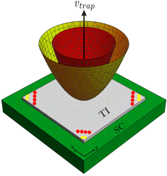
Figure 1: (Color online) Schematic picture of a 2D TI approximated by a high-temperature $d$-wave SC in the presence of two different 2D harmonic potentials, where the red paraboloid has larger potential magnitude than the yellow one. The Majorana zero modes are shown by red and yellow points. The number of MCSs (yellow points) are gradually increases as the HP magnitude increases which results in the formation of Majorana corner flat bands (red points).

An important issue is to both find and determine the robustness of the MCSs. As shown in Ref. Yan et al. (2018), the MCSs are robust in a 2D TI, also know as the quantum spin Hall insulator, in proximity with cuprate-based Zareapour et al. (2012); Li et al. (2015); Wang et al. (2013), or iron-based Stewart (2011); Xu et al. (2016); Wang et al. (2018c); Zhang et al. (2018) high-temperature SCs, as shown schematically in Fig. 1. In this system, modest edge imperfections do not affect the MCSs while big edge imperfections just create new corners that host their own MCSs. This study suggests that the shape of the system is important and it has some effects on the MCSs.

Here, we consider the harmonic potential (HP) as an example of a gradual confining potential. The HP is defined as $V_{i}=v_{\rm{trap}}\big{\{}(i_{x}-i^{c}_{x})^{2}+(i_{y}-i^{c}_{y})^{2}\big{\}}$ where $v_{\rm{trap}}$ is the potential magnitude, and $i^{c}=(i^{c}_{x},i^{c}_{y})$ is the coordinate of the central site of the square lattice which we take as the origin. There is no well-defined edge associated with a gradual confining potential and near a MCS, there is no additional corner where additional MCSs can appear. In the limit of a HP whose magnitude is much larger than the insulating gap, the region near the four corners of 2D TI in proximity with a $d$-wave SC becomes the location for unconventional superconductivity. It should be pointed out that in the homogeneous system by increasing the chemical potential there is a topological phase transition with bulk gap closing. Moreover, a time-reversal invariant (TRI) $d$-wave SC with [110] surface, has zero-energy flat dispersion due to a nontrivial one-dimensional (1D) winding number at a large enough chemical potential Sato et al. (2011); Wong and Law (2012); Wong et al. (2013); Nagai et al. (2017). Therefore, there might be a transition from MCSs to Majorana flat bands (MFBs) in a nonhomogeneous system with increasing the HP magnitude. The question arises: to what degree can the number of MCSs be varied as we change the magnitude of a confining potential? Will a topological phase transition occur as the bulk gap closes, or will there be a crossover as the bulk gap continues to decrease without closing?

In this paper, we show that in a second-order TSCs with a confining HP the MCSs-MFBs transition is merely a crossover: the number of the MZMs gradually increases while there is no 2D bulk gap closing as the HP magnitude increases. We find that the increase of the number of MZMs indicates the appearance of new Majorana states originating from the fact that only 1D gapped boundary modes become gapless without closing the bulk gap. This eventually leads to a new kind of MFBs which we call Majorana corner flat bands (MCFBs). It is found that 2D bulk states do not become gapless with increasing the HP magnitude in a system with open-boundary conditions (OBCs), i.e., the host system for the MCSs. We show that the crossover behavior is important for explaining the increase in the number of MZMs. In contrast, in a system with periodic boundary conditions (PBCs), the 2D bulk gap is closed if the potential magnitude at the corners, $v_{\rm{trap}}(r_{c})$, becomes larger than the insulating gap. We confirm that, under sharp potentials such as circular potential, the 2D bulk gap is closed in both OBCs and PBCs systems.

This paper is organized as follows. We introduce the model of a two-dimensional TI with a proximity-induced $d$-wave superconducting gap, as shown schematically in Fig. 1. This system hosts the MCSs when the chemical potential is smaller than the insulating gap Yan et al. (2018). Then, it will be shown that the MCSs-MCFBs transition in OBCs system is a crossover and there is no bulk gap closing as the HP magnitude increases. It will be proposed that this kind of MFB is new and different from the conventional one, which has already been reported along the [110] surface of a TRI 2D nodal $d$-wave SC Sato et al. (2011), in the sense that they only originate from MCSs or 1D gapped boundary states as illustrated in Fig. 2. Finally, we propose an experimental realization for observing this kind of MFB.

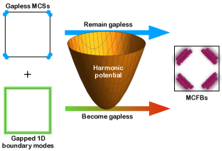
Figure 2: (Color online) A schematic picture of the procedure by which MCSs become MCFBs. (Left panel) There is no HP. The system has topologically distinct 1D gapped modes on the adjacent boundaries which leads to gapless MCSs at the intersection of two different boundaries, i.e., corners. (Right panel) After including the HP, the gapless MCSs remain gapless. However, the 1D gapped boundary modes become gapless modes.

II Formalism

The Bogoliubov-de Gennes (BdG) Hamiltonian of a 2D TI in proximity with a SC is given by,

$$\mathcal{H}=\frac{1}{2}\sum_{ij}\bm{\psi}^{\dagger}_{i}\begin{pmatrix}\hat{H}^{\rm N}_{ij}&&\hat{\Delta}_{ij}\\ \\ \hat{\Delta}_{ij}^{\dagger}&&-\hat{H}^{\rm N\ast}_{ij}\end{pmatrix}\bm{\psi}_{j},$$ (1)

with $\bm{\psi}^{\dagger}_{i}=(c^{\dagger}_{i,a,\uparrow},c^{\dagger}_{i,b,\uparrow},c^{\dagger}_{i,a,\downarrow},c^{\dagger}_{i,b,\downarrow},c_{i,a,\uparrow},c_{i,b,\uparrow},c_{i,a,\downarrow},c_{i,b,\downarrow})$. Here, $c^{\dagger}_{i,\alpha,\beta}(c_{i,\alpha,\beta})$ denotes the creation (annihilation) operator of an electron at site $i=(i_{x},i_{y})$, in orbital $\alpha$ = $a$ or $b$, with spin $\beta$ = $\uparrow$ or $\downarrow$. The normal state and superconducting parts of the Hamiltonian are given by $\hat{H}^{\rm N}_{ij}=m_{ij}\sigma_{z}s_{0}+A^{x}_{ij}\sigma_{x}s_{z}+A^{y}_{ij}\sigma_{y}s_{0}-\delta_{ij}(\mu-V_{i})\sigma_{0}s_{0}$, and $\hat{\Delta}_{ij}=-\text{i}\Delta_{ij}\sigma_{0}s_{y}$, respectively. The mass term is $m_{ij}=m_{0}\delta_{ij}-(t/2)(\delta_{i,i+\hat{x}}+\delta_{i,i-\hat{x}}+\delta_{i,i+\hat{y}}+\delta_{i,i-\hat{y}})$ where $m_{0}$ is on-site orbital-dependent energy, and $t$ is the intra-orbital nearest neighbor hopping magnitude along the $x$ and $y$ directions with unit vectors $\hat{x}$ and $\hat{y}$. The $\sigma_{x,y,z}$ and $s_{x,y,z}$ are Pauli matrices acting on orbital and spin degree of freedoms, respectively, and $\sigma_{0}$ and $s_{0}$ are $2\times 2$ unit matrices. Moreover, $A^{x}_{ij}=(-\text{i}\lambda/2)(\delta_{i,i+\hat{x}}-\delta_{i,i-\hat{x}})$, $A^{y}_{ij}=(-\text{i}\lambda/2)(\delta_{i,i+\hat{y}}-\delta_{i,i-\hat{y}})$ are the spin-orbit coupling terms with magnitude $\lambda$, where the symbol i denoting $\sqrt{-1}$ should not be confused with the site-index that generally occurs subscripted. The chemical potential is given by $\mu$ and $V_{i}$ is the 2D single particle potential magnitude at site $i$. The $d$-wave superconductivity order parameter with $d_{x^{2}-y^{2}}$ symmetry is expressed as $\Delta_{ij}=(\Delta_{d}/2)(\delta_{i,i+\hat{x}}+\delta_{i,i-\hat{x}}-\delta_{i,i+\hat{y}}-\delta_{i,i-\hat{y}})$.

In the absence of any single particle potential ($V_{i}=0$), the corresponding BdG Hamiltonian in momentum spacerem can be written as $\mathcal{H}=\sum_{\bm{k}}\Psi_{\bm{k}}^{\dagger}\mathcal{H}_{\text{BdG}}\Psi_{\bm{k}}/2$ where $\Psi_{\bm{k}}^{\dagger}=(c^{\dagger}_{\bm{k},a,\uparrow},c^{\dagger}_{\bm{k},b,\uparrow},c^{\dagger}_{\bm{k},a,\downarrow},c^{\dagger}_{\bm{k},b,\downarrow},c_{-\bm{k},a,\uparrow},c_{-\bm{k},b,\uparrow},c_{-\bm{k},a,\downarrow},c_{-\bm{k},b,\downarrow})$ and,

$$\mathcal{H}_{\text{BdG}}= ~{}m(\bm{k})\sigma_{z}s_{0}\tau_{z}+\lambda\sin k_{x}\sigma_{x}s_{z}\tau_{0}+\lambda\sin k_{y}\sigma_{y}s_{0}\tau_{z}$$

$$+\Delta(\bm{k})\sigma_{0}s_{y}\tau_{y}-\mu\sigma_{0}s_{0}\tau_{z},$$ (2)

where $\tau_{x,y,z}$ are Pauli matrices in particle-hole space, and $\tau_{0}$ is the $2\times 2$ unit matrix, and

$$\Delta(\bm{k})=\Delta_{d}(\cos k_{x}-\cos k_{y}),$$ (3)

$$m(\bm{k})=m_{0}-t(\cos k_{x}+\cos k_{y}).$$ (4)

The BdG Hamiltonian possesses both particle-hole symmetry (PHS), i.e., $\mathcal{P}\mathcal{H}^{\ast}_{\text{BdG}}(\bm{k})\mathcal{P}^{-1}=-\mathcal{H}_{\text{BdG}}(-\bm{k})$ where $\mathcal{P}=\sigma_{0}s_{0}\tau_{x}$, and time-reversal symmetry (TRS), i.e., $\mathcal{T}\mathcal{H}^{\ast}_{\text{BdG}}(\bm{k})\mathcal{T}^{-1}=\mathcal{H}_{\text{BdG}}(-\bm{k})$ where $\mathcal{T}=i\sigma_{0}s_{y}\tau_{0}$. The combination of these two anti-unitary symmetries gives rise to a unitary chiral symmetry, i.e., $\mathcal{S}\mathcal{H}_{\text{BdG}}(\bm{k})\mathcal{S}^{-1}=-\mathcal{H}_{\text{BdG}}(\bm{k})$ where $\mathcal{S}=-i\mathcal{P}\mathcal{T}$. The intrinsic particle-hole symmetry of the BdG Hamiltonian guarantees that the eigenstates whose eigenvalues are zero satisfy the Majorana conditions as discussed in the Appendix. It should be noted that the above Hamiltonian without $d$-wave pairing becomes the paradigmatic Bernevig-Hughes-Zhang (BHZ) model of 2D TIs Bernevig et al. (2006). In addition, the normal state dispersion is given as

$$E(\bm{k})=\pm\sqrt{m^{2}(\bm{k})+\lambda^{2}(\sin^{2}k_{x}+\sin^{2}k_{y})}-\mu,$$ (5)

so, the insulating gap as an important quantity in our analysis, is given by $|m(\bm{k}=0)|=|m_{0}-2t|$. Through this work, we set $m_{0}=1.5$, $\mu=0$, $t=\lambda=1$, and $\Delta_{d}=0.5$.

III Results

III.1 Robustness of MCSs and crossover with MCFBs

In a TRI system, MCSs manifest themselves as Majorana Kramers pairs which are protected zero-energy modes localized at the four corners of the 2D TI in proximity with a $d$-wave. By adding proximity-induced $d$-wave superconductivity, the helical gapless boundary modes of the 2D TI become gapped, so in our system as a 2D square sample, there are 1D gapped localized modes along the four boundaries when the chemical potential is smaller than the insulating gap. By constructing the low-energy Hamiltonian and through the use of localized modes, we can define the topological invariant, which depends on the direction of a boundary Yan et al. (2018). There should be gapless zero modes at four intersections or corners of the 2D TI known as MCSs Since the 1D effective systems along the vertical and horizontal boundaries have different topological invariants or Dirac masses,

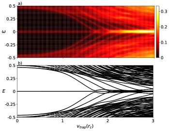
Figure 3: (Color online) (a) Density of states, and (b) eigenvalues of the BdG Hamiltonian as a function of $v_{\rm{trap}}(r_{c})$ for a $51\times 51$ square lattice with OBCs. The unit of all values is $|m(\bm{k}=0)|$.

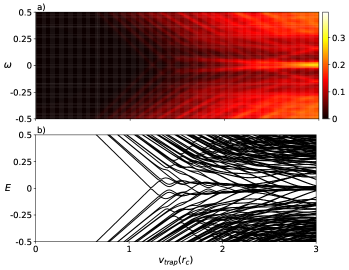
Figure 4: (Color online) (a) Density of states, and (b) eigenvalues of the BdG Hamiltonian as a function of $v_{\rm{trap}}(r_{c})$ for a $51\times 51$ square lattice with PBCs. The unit of all values is $|m(\bm{k}=0)|$.

We argue that in a second-order TSC, the MCSs-MCFBs transition is actually a crossover in the OBCs system with increasing the HP magnitude: the number of MZMs gradually increases while there is no bulk gap closing as is illustrated in Fig. 3. It can be seen that there are branches of eigenvalues whose values decrease from 0.5 with increasing the HP magnitude although the bulk gap remains open. We find that the proliferation of the MZMs originate from the fact that only 1D gapped boundary modes becomes gapless without the 2D bulk gap closing.

In contrast, in the PBCs system with an increasing HP magnitude, the 2D bulk gap is closed if the potential magnitude at the four corners [$v_{\rm{trap}}(r_{c})$] of the 2D TI becomes larger than the insulating gap as shown in Fig. 4. In this case, by increasing the HP magnitude there are no MZMs because there are no 1D gapped boundary modes to become gapless. We have verified that the same behavior persists for larger systems.

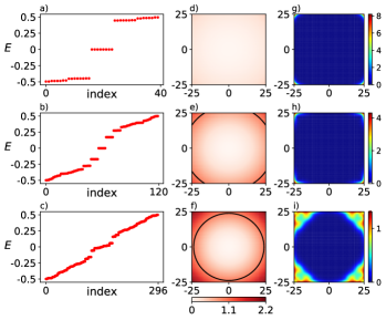
Figure 5: (Color online) (a,b,c) Eigenvalues of the BdG Hamiltonian, (d,e,f) two-dimension harmonic potential, and (g,h,i) zero-energy local density of states for a $51\times 51$ square lattice with OBCs in the presence of three different HP magnitudes $v_{\rm{trap}}(r_{c})$ = 0.4 (a,d,g), 1.4 (b,e,h), and 2.2 (c,f,i). Outside the two black circles $v_{\rm{trap}}(r_{c})>|m(\bm{k}=0)|$, i.e., the HP magnitude is larger than the insulating gap locally. Both the eigenvalues and HP magnitude are given in units of $|m(\bm{k}=0)|$. The smearing factor in the Lorentzian function for plotting the local density of states is 0.005.

To see the MCSs-MCFBs transition in more detail, we show the real space dependence of the zero-energy local density of states in Fig. 5. In the region outside the black circles of the two lower middle panels of this figure, the HP magnitude is larger than the insulating gap locally, so Figs. 5(b), 5(e), and 5(h) indicate that MCSs are robust even outside this circle. Moreover, the region outside the circles can host MCFBs, and the additional MZMs originate from only 1D gapped boundary modes that become gapless.

III.2 Flatness and the origin of MCFBs

It should be noted that an exact zero-energy eigenvalue cannot be obtained in the theoretical calculations for a finite system because of finite size effects. Thus, zero energy have to be defined. An eigenvalue can be considered as a zero-energy mode in such a finite system if its magnitude is very small. Therefore, the eigenvalue $E_{i}$ can be considered as a zero-energy eigenvalue if it satisfies $|E_{i}|\leq\varepsilon$ condition for a very small $\varepsilon$. By using of this definition for zero-energy modes, we show that as the harmonic trap magnitude is increased, the number of zero-energy eigenvalue increases independent of the value of $\varepsilon$ for large enough lattice. In Fig. 6, the ratio between the number of eigenvalues inside the $|E_{i}|\leq\varepsilon$ interval, say $N_{f}$, and the number of boundary states, which is proportional to the size of the lattice along $x$ or $y$-direction, is plotted. This figure clearly illustrates that this ratio is increasing in the thermodynamic limit, and a truly flat band appears by increasing harmonic trap magnitude if finite-size effects are suppressed.

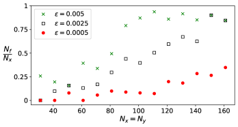
Figure 6: (Color online) The ratio between the number of eigenvalues inside the $|E_{i}|\leq\varepsilon$ interval and the $N_{x}$ as a function of the size of the boundaries of the lattice for the OBCs at three different values of $\varepsilon$ with $v_{\rm{trap}}(r_{c})=1.1|m(\bm{k}=0)|$.

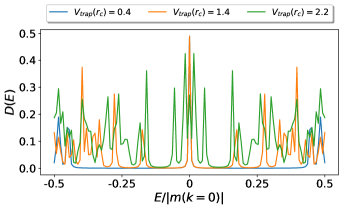
Figure 7: (Color online) Density of states as a function of energy in the unit of insulating gap value for the same parameters as the Fig. 5. The bulk gap remains open as harmonic potential magnitude increases in the weak potential limit.

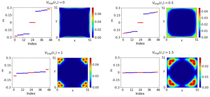
Figure 8: (Color online) Eigenvalues of the BdG Hamiltonian and the square of the wave function’s amplitude for different values of $v_{\rm{trap}}(r_{c})$ and for a $51\times 51$ square lattice with OBCs. The square of the wave function’s amplitude is plotted only for the eigenvalues that are denoted with blue color. They are gapped boundary states that become gapless by increasing the HP magnitude.

In Fig. 7, we plot the density of states (DOS) for the same parameters as in Fig. 5. It can be clearly seen that the number of Majorana zero modes increases without the bulk gap closing as the harmonic potential magnitude increases in the weak potential limit. The states that appear close to zero energy in this figure are boundary states not bulk states according to Fig. 8, where the origin of MCFBs is shown. In Fig. 8, we show that MCFBs originate from only gapped states localized at one-dimensional (1D) boundaries. In this figure we plot the square of the wave function’s amplitude associated with only blue points. As the HP magnitude is increased, the energy corresponding to these 1D boundary states become smaller, and they become more localized around the corners. By increasing the HP magnitude, more and more 1D gapped modes become gapless.

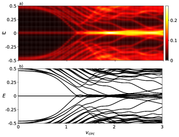
Figure 9: (Color online) (a) Density of states, and (b) eigenvalues of the BdG Hamiltonian as a function of $v_{\rm circ}$ for a $51\times 51$ square lattice with OBCs. The unit of all values is $|m(\bm{k}=0)|$.

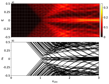
Figure 10: (Color online) (a) Density of states, and (b) eigenvalues of the BdG Hamiltonian as a function of $v_{\rm circ}$ for a $51\times 51$ square lattice with PBCs. The unit of all values is $|m(\bm{k}=0)|$.

III.3 Circular potential

Let us define the circular potential as $V_{i}=v_{\rm circ}$ for $(i_{x}-i^{c}_{x})^{2}+(i_{y}-i^{c}_{y})^{2}>R^{2}$ where $v_{\rm circ}$ is the strength of the circular potential, and $i^{c}=(i^{c}_{x},i^{c}_{y})$ is the coordinate of the central site of a 2D sample. Here, we take $R=N_{x}/2$ where $N_{x}$ is the number of sites along $x$-axis direction. As shown in Figs. 9 and 10, the bulk gap closes in both OBCs and PBCs for a circular potential, so there is no crossover and no MCFBs in the presence of a circular potential which is not similar to the case of the harmonic potential.

IV Discussion

Let us discuss the difference between conventional MFBs in a $d$-wave SC and MCFBs in our system. In a SC with order parameter symmetry $d_{x^{2}-y^{2}}$, it is well known that there are Andreev flat bound states, which appear at the [110] surface. On the other hand, there is no zero-energy bound state at the [100] and [010] surfaces Daido and Yanase (2017); Kashiwaya et al. (1995). For this nodal SC, it is possible to define a 1D partial Brillouin zone by fixing the $(d-1)$-dimensional momentum $\bm{k}_{||}$ at a certain point Sato et al. (2011); Daido and Yanase (2017); Yada et al. (2011); Schnyder and Ryu (2011). As long as the pair potential in such a partial Brillouin zone (BZ) is fully gapped, we can define the one-dimensional winding number as the topological invariant of a nodal TSC:

$$\mathcal{W}(\bm{k_{||}})=\frac{1}{2\pi}~{}\text{Im}\int dk_{\perp}\partial_{k_{\perp}}\ln\det(q),$$ (6)

where $k_{\perp}$ is the momentum in a one-dimensional BZ, and $\bm{k}_{||}$ is the momentum parallel to the surface that we consider. Moreover, in Eq. (6), $q(\bm{k})$ is the off-diagonal block of the BdG Hamiltonian in the basis that diagonalizes the chiral symmetry operator such that $\det q(\bm{k})=\big{\{}m^{2}(\bm{k})+(\Delta(\bm{k})+i\mu)^{2}+\lambda^{2}\sin^{2}k_{x}+\lambda^{2}\sin^{2}k_{y}\big{\}}^{2}$. For a finite winding number, there are $|\mathcal{W}(\bm{k_{||}})|$-fold degenerate zero-energy modes at a surface parallel to $\bm{k_{||}}$. Such highly degenerate surface bound states are known as Majorana flat bands (MFBs) because the energy dispersion is independent of $\bm{k_{||}}$ Ikegaya et al. (2018).

A 2D homogeneous TI in proximity with a $d$-wave SC becomes SC with increasing chemical potential. This transition is a topological phase transition with bulk gap closing since a $d$-wave SC order parameter has line nodes. In this homogeneous system with large enough chemical potential, there are MFBs at the [110] surface because of nontrivial value of winding number. The origin of these MFBs are Andreev bound states Sato et al. (2011). However, here we find that in the case of MCFBs not only is there no 2D bulk gap closing in the OBCs system with increasing harmonic potential magnitude, but also the number of MZMs increases only because of the reduction of the energy of the 1D boundary gapped modes. Also note that although MCSs are exponentially localized at the corners of the system, MCFBs are localized very close to the four corners in the weak potential limit.

Although MCFBs consist of many very spatially close MZMs, they cannot hybridize and become gapped out. This is in contrast to the fact that MCSs hybridize and annihilate if they are brought close together. The reasons for the weak hybridization can naturally be explained by the use of the 1D boundary modes, time-reversal symmetry, and the crossover behavior as follows. Without a confining potential, the wave function of MCSs and 1D gapped boundary modes are orthogonal because they are eigenvectors of the BdG Hamiltonian with different energies. The wave functions gradually change with changing the HP magnitude and remain orthogonal since there is no bulk gap closing. Therefore, the crossover makes the MCFBs stable by preserving the orthogonality of these wave functions. In addition, it is known that both Majorana flat bands in a $d$-wave SC, and Majorana corner states in a second-order TSC are protected by time-reversal symmetry Sato et al. (2011); Yan et al. (2018). In our system, in zero and strong potential limits, the system is second-order TSC and $d$-wave SC, respectively. Therefore, the time-reversal symmetry protects the Majorana corner flat bands in the weak potential limit since this phenomenon is a crossover.

V Conclusions

It has been recently proposed that a second-order TSC hosts Majorana corner states (MCSs) localized at the four corners of a 2D TI in proximity with some unconventional high-temperature SCs. This work provides a theoretical framework to make only 1D gapped boundary modes gapless without closing the bulk gap in 2D second-order TSCs. Second-order TSCs always have $(d-1)$-dimensional gapped boundary modes and $(d-2)$-dimensional gapless modes in $d$-spatial dimensions. Our results suggest that increasing the gradual potential magnitude proliferates the number of MCSs by making only 1D gapped boundary modes gapless without closing the bulk gap. This finally leads to a new kind of MFB, namely Majorana corner flat bands (MCFBs). In contrast to the conventional mechanism, MCFBs cannot be characterized by a 1D winding number and only originate from 1D gapped boundary modes that become gapless without closing the bulk gap.

It also has been shown that the presence of time-reversal symmetry during the MCSs-MCFBs crossover prevent MCSs from hybridizing and protect MCFBs. There might be a topological invariant for this particular inhomogeneous system to characterize the crossover, but finding that in real-space is a mathematically challenging task and beyond the scope of our present paper.

In experiment, if one can observe the MCSs in second-order TSCs, such as a hybrid structure of TI and an unconventional SC or even cold atom systems, one can also observe the MCSs-MCFBs crossover and MCFBs with adding a gradual potential such as HP. More precisely speaking, for having a hybrid structure of TI and an unconventional SC, a monolayer of WTe₂ as a high-temperature topological insulator Qian et al. (2014); Wu et al. (2018) can be exploited in proximity to a $d$-wave high-temperature cuprate superconductor. In this hybrid solid-state systems, some potentials can be applied by using of electron double-layer transistors (EDLTs) Li et al. (2016); Ahn et al. (2006); Weisheit et al. (2007), which can be used to apply an electric field to the sample. Normally the potentials generated by the EDLT techniques have sharp edges. Nevertheless, there might be some possibilities in the future or other advanced techniques to control the sharpness of this trapping potential in order to approach a harmonic potential. This work might open up new prospects for realizing MZMs and its applications in quantum computation and information, which will be left for future investigations.

*

Appendix A Majorana Condition

Although the BdG Hamiltonian in Eq. (1) of the main paper is a $8N\times 8N$ matrix, by changing the basis it can be written as a block diagonal matrix where each block is a $4N\times 4N$ matrix and $N$ is the number of lattice sites. In this section, it is shown that the zero modes of each of these $4N\times 4N$ blocks meets the Majorana conditions. The Hamiltonian can be rewritten as,

$${\cal H}=\frac{1}{2}\Psi^{\dagger}\hat{H}\Psi,$$ (7)

here $\bm{\psi}^{\dagger}_{i}=(c^{\dagger}_{i,a,\uparrow},c^{\dagger}_{i,b,\uparrow},c^{\dagger}_{i,a,\downarrow},c^{\dagger}_{i,b,\downarrow},c_{i,a,\uparrow},c_{i,b,\uparrow},c_{i,a,\downarrow},c_{i,b,\downarrow})$ and,

$$\hat{H} =\left(\begin{array}[]{cc}H_{n}&\Delta\\ \Delta^{\dagger}&-H_{n}^{\ast}\end{array}\right),$$ (10)

where

$$H_{n}=\left(\begin{array}[]{cc}H_{1}&0\\ 0&H_{2}\end{array}\right),\hskip 14.22636pt\Delta=\left(\begin{array}[]{cc}0&-\Delta\\ \Delta&0\end{array}\right).$$ (15)

The BdG equations are

$$\hat{H}\left(\begin{array}[]{c}\vec{u}_{1}\\ \vec{u}_{2}\\ \vec{v}_{1}\\ \vec{v}_{2}\end{array}\right) =E\left(\begin{array}[]{c}\vec{u}_{1}\\ \vec{u}_{2}\\ \vec{v}_{1}\\ \vec{v}_{2}\end{array}\right),$$ (24)

or

$$H_{1}\vec{u}_{1}-\Delta\vec{v}_{2} =E\vec{u}_{1}$$ (25)

$$H_{2}\vec{u}_{2}+\Delta\vec{v}_{1} =E\vec{u}_{2}$$ (26)

$$\Delta^{\ast}\vec{u}_{2}-H_{1}^{\ast}\vec{v}_{1} =E\vec{v}_{1}$$ (27)

$$-\Delta^{\ast}\vec{u}_{1}-H_{2}^{\ast}\vec{v}_{2} =E\vec{v}_{2}.$$ (28)

So, we have a $4N\times 4N$ matrix:

$$\left(\begin{array}[]{cc}H_{1}&-\Delta\\ -\Delta^{\ast}&-H_{2}^{\ast}\end{array}\right)\left(\begin{array}[]{c}\vec{u}_{1}\\ \vec{v}_{2}\end{array}\right) =E\left(\begin{array}[]{c}\vec{u}_{1}\\ \vec{v}_{2}\end{array}\right).$$ (35)

Then, it can be shown that,

$$-H_{1}^{\ast}\vec{u}_{1}^{\ast}+\Delta^{\ast}\vec{v}_{2}^{\ast} =-E\vec{u}_{1}^{\ast}$$ (36)

$$-H_{2}^{\ast}\vec{u}_{2}^{\ast}-\Delta^{\ast}\vec{v}_{1}^{\ast} =-E\vec{u}_{2}^{\ast}$$ (37)

$$-\Delta\vec{u}_{2}^{\ast}+H_{1}\vec{v}_{1}^{\ast} =-E\vec{v}_{1}^{\ast}$$ (38)

$$\Delta\vec{u}_{1}^{\ast}+H_{2}\vec{v}_{2}^{\ast} =-E\vec{v}_{2}^{\ast}$$ (39)

or

$$\hat{H}\left(\begin{array}[]{c}\vec{v}_{1}^{\ast}\\ \vec{v}_{2}^{\ast}\\ \vec{u}_{1}^{\ast}\\ \vec{u}_{2}^{\ast}\end{array}\right) =-E\left(\begin{array}[]{c}\vec{v}_{1}^{\ast}\\ \vec{v}_{2}^{\ast}\\ \vec{u}_{1}^{\ast}\\ \vec{u}_{2}^{\ast}\end{array}\right).$$ (48)

Therefore, if $(\vec{u}_{1}^{i},\vec{u}_{2}^{i},\vec{v}_{1}^{i},\vec{v}_{2}^{i})$ is an eigenstate with energy $E_{i}$, then $(\vec{v}_{1}^{i\ast},\vec{v}_{2}^{i\ast},\vec{u}_{1}^{i\ast},\vec{u}_{2}^{i\ast})$ is an eigenstate with energy $-E_{i}$ which should be expected because of particle-hole symmetry. This means that if $E=0$, we have the following relations,

$$\vec{u}_{1}^{i}=\vec{v}_{1}^{i\ast}\hskip 42.67912pt\vec{u}_{2}^{i} =\vec{v}_{2}^{i\ast}.$$ (49)

In other words, if we have $(\vec{u}_{1}^{i},\vec{v}_{2}^{i})$ with the energy $E_{i}$, we can obtain eigenstates $(\vec{u}_{2}^{i},\vec{v}_{1}^{i})=(\vec{v}_{2}^{i\ast},\vec{u}_{1}^{i\ast})$ with the energy $-E_{i}$. It means by finding only the eigenvalues and eigenstates of the $4N\times 4N$ Hamiltonian in Eq. (35), one can find all eigenvalues and eigenstates of the $8N\times 8N$ Hamiltonian in Eq. (10) much more easily due to the particle-hole symmetry. In the rest of this section, we will show that all the zero modes of the $4N\times 4N$ Hamiltonian satisfy Majorana conditions.

The unitary matrix that diagonalizes the matrix $\hat{H}$ is expressed as

$$\hat{U}=\left(\begin{array}[]{cc}\hat{u}&\hat{v}^{\ast}\\ \hat{v}&\hat{u}^{\ast}\end{array}\right),\hskip 11.38092pt\hat{H}=\hat{U}\left(\begin{array}[]{cc}\hat{E}&0\\ 0&-\hat{E}\end{array}\right)\hat{U}^{\dagger}$$ (54)

where

$$\hat{u}\equiv\left(\begin{array}[]{ccc}\vec{u}_{1}^{1}&\cdots&\vec{u}_{1}^{N}\\ \vec{u}_{2}^{2}&\cdots&\vec{u}_{2}^{N}\end{array}\right),\hskip 11.38092pt\hat{v}\equiv\left(\begin{array}[]{ccc}\vec{v}_{1}^{1}&\cdots&\vec{v}_{1}^{N}\\ \vec{v}_{2}^{2}&\cdots&\vec{v}_{2}^{N}\end{array}\right).$$ (59)

So,

$${\cal H} =\frac{1}{2}\Psi^{\dagger}\hat{U}\left(\begin{array}[]{cc}\hat{E}&0\\ 0&-\hat{E}\end{array}\right)\hat{U}^{\dagger}\Psi$$ (62)

$$=\frac{1}{2}\sum_{i}(E_{i}\gamma_{i}^{\dagger}\gamma_{i}-E_{i}\gamma_{i}\gamma_{i}^{\dagger}),$$ (63)

where

$$\left(\begin{array}[]{c}\vec{\gamma}\\ \vec{\gamma^{\dagger}}\end{array}\right) =\hat{U}^{\dagger}\left(\begin{array}[]{c}\vec{c}\\ \vec{c^{\dagger}}\end{array}\right)$$ (68)

or

$$\gamma_{i} =\sum_{l}\left[[\hat{u}]_{li}^{\ast}c_{l}+[\hat{v}]_{li}^{\ast}c_{l}^{\dagger}\right]$$ (69)

$$\gamma_{i}^{\dagger} =\sum_{l}\left[[\hat{u}]_{li}c_{l}^{\dagger}+[\hat{v}]_{li}c_{l}\right].$$ (70)

It is obvious that $\gamma_{i}^{\dagger}\neq\gamma_{i}$. However, we have two special conditions for only zero-eigenvalues which is Eq. (49). Using them we will have,

$$\gamma_{i}^{\dagger} =\sum_{l}\left[[\hat{v}]_{li}^{\ast}c_{l}^{\dagger}+[\hat{u}]_{li}^{\ast}c_{l}\right]=\gamma_{i}.$$ (71)

Therefore, the zero-energy eigenstates are all Majorana.

References

- Qi and Zhang (2011) Xiao-Liang Qi and Shou-Cheng Zhang, “Topological insulators and superconductors,” Reviews of Modern Physics 83, 1057 (2011).
- Hasan and Kane (2010) M Zahid Hasan and Charles L Kane, “Colloquium: topological insulators,” Reviews of Modern Physics 82, 3045 (2010).
- Moore (2010) Joel E Moore, “The birth of topological insulators,” Nature 464, 194 (2010).
- Sato and Ando (2017) Masatoshi Sato and Yoichi Ando, “Topological superconductors: a review,” Reports on Progress in Physics 80, 076501 (2017).
- Qi et al. (2009) Xiao-Liang Qi, Taylor L Hughes, Srinivas Raghu, and Shou-Cheng Zhang, “Time-reversal-invariant topological superconductors and superfluids in two and three dimensions,” Physical review letters 102, 187001 (2009).
- Qi et al. (2010) Xiao-Liang Qi, Taylor L Hughes, and Shou-Cheng Zhang, “Topological invariants for the Fermi surface of a time-reversal-invariant superconductor,” Physical Review B 81, 134508 (2010).
- Zhang et al. (2013a) Fan Zhang, CL Kane, and EJ Mele, “Time-reversal-invariant topological superconductivity and Majorana Kramers pairs,” Physical review letters 111, 056402 (2013a).
- Wong and Law (2012) Chris LM Wong and Kam Tuen Law, “Majorana Kramers doublets in -wave superconductors with rashba spin-orbit coupling,” Physical Review B 86, 184516 (2012).
- Sato (2010) Masatoshi Sato, “Topological odd-parity superconductors,” Physical Review B 81, 220504 (2010).
- Zhang et al. (2013b) Fan Zhang, CL Kane, and EJ Mele, “Topological mirror superconductivity,” Physical review letters 111, 056403 (2013b).
- Haim et al. (2016) Arbel Haim, Erez Berg, Karsten Flensberg, and Yuval Oreg, “No-go theorem for a time-reversal invariant topological phase in noninteracting systems coupled to conventional superconductors,” Physical Review B 94, 161110 (2016).
- Benalcazar et al. (2017a) Wladimir A Benalcazar, B Andrei Bernevig, and Taylor L Hughes, “Quantized electric multipole insulators,” Science 357, 61–66 (2017a).
- Benalcazar et al. (2017b) Wladimir A Benalcazar, B Andrei Bernevig, and Taylor L Hughes, “Electric multipole moments, topological multipole moment pumping, and chiral hinge states in crystalline insulators,” Physical Review B 96, 245115 (2017b).
- Schindler et al. (2018a) Frank Schindler, Ashley M Cook, Maia G Vergniory, Zhijun Wang, Stuart SP Parkin, B Andrei Bernevig, and Titus Neupert, “Higher-order topological insulators,” Science advances 4, eaat0346 (2018a).
- Langbehn et al. (2017) Josias Langbehn, Yang Peng, Luka Trifunovic, Felix von Oppen, and Piet W Brouwer, “Reflection-symmetric second-order topological insulators and superconductors,” Physical review letters 119, 246401 (2017).
- Ezawa (2018) Motohiko Ezawa, “Higher-order topological insulators and semimetals on the breathing kagome and pyrochlore lattices,” Physical review letters 120, 026801 (2018).
- Khalaf (2018) Eslam Khalaf, “Higher-order topological insulators and superconductors protected by inversion symmetry,” Physical Review B 97, 205136 (2018).
- Geier et al. (2018) Max Geier, Luka Trifunovic, Max Hoskam, and Piet W Brouwer, “Second-order topological insulators and superconductors with an order-two crystalline symmetry,” Physical Review B 97, 205135 (2018).
- Imhof et al. (2018) Stefan Imhof, Christian Berger, Florian Bayer, Johannes Brehm, Laurens W Molenkamp, Tobias Kiessling, Frank Schindler, Ching Hua Lee, Martin Greiter, Titus Neupert, et al., “Topolectrical-circuit realization of topological corner modes,” Nature Physics 14, 925 (2018).
- Franca et al. (2018) S Franca, J van den Brink, and IC Fulga, “An anomalous higher-order topological insulator,” Physical Review B 98, 201114 (2018).
- Călugăru et al. (2019) Dumitru Călugăru, Vladimir Juričić, and Bitan Roy, “Higher-order topological phases: A general principle of construction,” Physical Review B 99, 041301 (2019).
- Read and Green (2000) Nicholas Read and Dmitry Green, “Paired states of fermions in two dimensions with breaking of parity and time-reversal symmetries and the fractional quantum hall effect,” Physical Review B 61, 10267 (2000).
- Volovik (1999) GE Volovik, “Fermion zero modes on vortices in chiral superconductors,” Journal of Experimental and Theoretical Physics Letters 70, 609–614 (1999).
- Kitaev (2001) A Yu Kitaev, “Unpaired Majorana fermions in quantum wires,” Physics-Uspekhi 44, 131 (2001).
- Alicea (2012) Jason Alicea, “New directions in the pursuit of Majorana fermions in solid state systems,” Reports on progress in physics 75, 076501 (2012).
- Lian et al. (2018) Biao Lian, Xiao-Qi Sun, Abolhassan Vaezi, Xiao-Liang Qi, and Shou-Cheng Zhang, “Topological quantum computation based on chiral Majorana fermions,” Proceedings of the National Academy of Sciences 115, 10938–10942 (2018).
- Schindler et al. (2018b) Frank Schindler, Zhijun Wang, Maia G Vergniory, Ashley M Cook, Anil Murani, Shamashis Sengupta, Alik Yu Kasumov, Richard Deblock, Sangjun Jeon, Ilya Drozdov, et al., “Higher-order topology in bismuth,” Nature Physics 14, 918 (2018b).
- Ghorashi et al. (2019) Sayed Ali Akbar Ghorashi, Xiang Hu, Taylor L. Hughes, and Enrico Rossi, “Second-order dirac superconductors and magnetic field induced Majorana hinge modes,” Phys. Rev. B 100, 020509 (2019).
- Lee et al. (2006) Patrick A Lee, Naoto Nagaosa, and Xiao-Gang Wen, “Doping a mott insulator: Physics of high-temperature superconductivity,” Reviews of modern physics 78, 17 (2006).
- Sigrist and Ueda (1991) Manfred Sigrist and Kazuo Ueda, “Phenomenological theory of unconventional superconductivity,” Reviews of Modern physics 63, 239 (1991).
- Wu et al. (2019) Zhigang Wu, Zhongbo Yan, and Wen Huang, “Higher-order topological superconductivity: Possible realization in Fermi gases and \ceSr2RuO4,” Physical Review B 99, 020508 (2019).
- Yan et al. (2018) Zhongbo Yan, Fei Song, and Zhong Wang, “Majorana Kramers pairs in a high-temperature platform,” Physical review letters 121, 096803 (2018).
- Wang et al. (2018a) Qiyue Wang, Cheng-Cheng Liu, Yuan-Ming Lu, and Fan Zhang, “High-temperature Majorana corner states,” Physical review letters 121, 186801 (2018a).
- Hsu et al. (2018) Chen-Hsuan Hsu, Peter Stano, Jelena Klinovaja, and Daniel Loss, “Majorana Kramers pairs in higher-order topological insulators,” Physical review letters 121, 196801 (2018).
- Zeng et al. (2019) Chuanchang Zeng, T. D. Stanescu, Chuanwei Zhang, V. W. Scarola, and Sumanta Tewari, “Majorana corner modes with solitons in an attractive hubbard-hofstadter model of cold atom optical lattices,” Physical review letters 123, 060402 (2019).
- Liu et al. (2018) Tao Liu, James Jun He, and Franco Nori, “Majorana corner states in a two-dimensional magnetic topological insulator on a high-temperature superconductor,” Physical Review B 98, 245413 (2018).
- Volpez et al. (2019) Yanick Volpez, Daniel Loss, and Jelena Klinovaja, “Second-order topological superconductivity in -junction Rashba layers,” Physical review letters 122, 126402 (2019).
- Zhu (2018) Xiaoyu Zhu, “Tunable Majorana corner states in a two-dimensional second-order topological superconductor induced by magnetic fields,” Physical Review B 97, 205134 (2018).
- Wang et al. (2018b) Yuxuan Wang, Mao Lin, and Taylor L Hughes, “Weak-pairing higher order topological superconductors,” Physical Review B 98, 165144 (2018b).
- Zareapour et al. (2012) Parisa Zareapour, Alex Hayat, Shu Yang F Zhao, Michael Kreshchuk, Achint Jain, Daniel C Kwok, Nara Lee, Sang-Wook Cheong, Zhijun Xu, Alina Yang, et al., “Proximity-induced high-temperature superconductivity in the topological insulators \ceBi2Se3 and \ceBi2Te3,” Nature communications 3, 1056 (2012).
- Li et al. (2015) Zi-Xiang Li, Cheung Chan, and Hong Yao, “Realizing Majorana zero modes by proximity effect between topological insulators and -wave high-temperature superconductors,” Physical Review B 91, 235143 (2015).
- Wang et al. (2013) Eryin Wang, Hao Ding, Alexei V Fedorov, Wei Yao, Zhi Li, Yan-Feng Lv, Kun Zhao, Li-Guo Zhang, Zhijun Xu, John Schneeloch, et al., “Fully gapped topological surface states in \ceBi2Se3 films induced by a d-wave high-temperature superconductor,” Nature physics 9, 621 (2013).
- Stewart (2011) GR Stewart, “Superconductivity in iron compounds,” Reviews of Modern Physics 83, 1589 (2011).
- Xu et al. (2016) Gang Xu, Biao Lian, Peizhe Tang, Xiao-Liang Qi, and Shou-Cheng Zhang, “Topological superconductivity on the surface of Fe-based superconductors,” Physical review letters 117, 047001 (2016).
- Wang et al. (2018c) Dongfei Wang, Lingyuan Kong, Peng Fan, Hui Chen, Shiyu Zhu, Wenyao Liu, Lu Cao, Yujie Sun, Shixuan Du, John Schneeloch, et al., “Evidence for Majorana bound states in an iron-based superconductor,” Science 362, 333–335 (2018c).
- Zhang et al. (2018) Peng Zhang, Koichiro Yaji, Takahiro Hashimoto, Yuichi Ota, Takeshi Kondo, Kozo Okazaki, Zhijun Wang, Jinsheng Wen, GD Gu, Hong Ding, et al., “Observation of topological superconductivity on the surface of an iron-based superconductor,” Science 360, 182–186 (2018).
- Sato et al. (2011) Masatoshi Sato, Yukio Tanaka, Keiji Yada, and Takehito Yokoyama, “Topology of Andreev bound states with flat dispersion,” Physical Review B 83, 224511 (2011).
- Wong et al. (2013) Chris LM Wong, Jie Liu, KT Law, and Patrick A Lee, “Majorana flat bands and unidirectional Majorana edge states in gapless topological superconductors,” Physical Review B 88, 060504 (2013).
- Nagai et al. (2017) Yuki Nagai, Yukihiro Ota, and K Tanaka, “Time-reversal symmetry breaking and gapped surface states due to spontaneous emergence of new order in d-wave nanoislands,” Physical Review B 96, 060503 (2017).
- (50) This assumes translational invariance, which precludes the realistic possibility that the order parameter changes near the surface of a material compared to the bulk, for example.
- Bernevig et al. (2006) B Andrei Bernevig, Taylor L Hughes, and Shou-Cheng Zhang, “Quantum spin hall effect and topological phase transition in hgte quantum wells,” Science 314, 1757–1761 (2006).
- Daido and Yanase (2017) Akito Daido and Youichi Yanase, “Majorana flat bands, chiral Majorana edge states, and unidirectional Majorana edge states in noncentrosymmetric superconductors,” Physical Review B 95, 134507 (2017).
- Kashiwaya et al. (1995) Satoshi Kashiwaya, Yukio Tanaka, Masao Koyanagi, Hiroshi Takashima, and Koji Kajimura, “Origin of zero-bias conductance peaks in high- superconductors,” Physical Review B 51, 1350 (1995).
- Yada et al. (2011) Keiji Yada, Masatoshi Sato, Yukio Tanaka, and Takehito Yokoyama, “Surface density of states and topological edge states in noncentrosymmetric superconductors,” Physical Review B 83, 064505 (2011).
- Schnyder and Ryu (2011) Andreas P Schnyder and Shinsei Ryu, “Topological phases and surface flat bands in superconductors without inversion symmetry,” Physical Review B 84, 060504 (2011).
- Ikegaya et al. (2018) Satoshi Ikegaya, Shingo Kobayashi, and Yasuhiro Asano, “Symmetry conditions of a nodal superconductor for generating robust flat-band Andreev bound states at its dirty surface,” Physical Review B 97, 174501 (2018).
- Qian et al. (2014) Xiaofeng Qian, Junwei Liu, Liang Fu, and Ju Li, “Quantum spin hall effect in two-dimensional transition metal dichalcogenides,” Science 346, 1344–1347 (2014).
- Wu et al. (2018) Sanfeng Wu, Valla Fatemi, Quinn D Gibson, Kenji Watanabe, Takashi Taniguchi, Robert J Cava, and Pablo Jarillo-Herrero, “Observation of the quantum spin hall effect up to 100 kelvin in a monolayer crystal,” Science 359, 76–79 (2018).
- Li et al. (2016) LJ Li, ECT O’Farrell, KP Loh, Goki Eda, B Özyilmaz, and AH Castro Neto, “Controlling many-body states by the electric-field effect in a two-dimensional material,” Nature 529, 185 (2016).
- Ahn et al. (2006) CH Ahn, A Bhattacharya, M Di Ventra, James N Eckstein, C Daniel Frisbie, ME Gershenson, AM Goldman, IH Inoue, Jochen Mannhart, Andrew J Millis, et al., “Electrostatic modification of novel materials,” Reviews of Modern Physics 78, 1185 (2006).
- Weisheit et al. (2007) Martin Weisheit, Sebastian Fähler, Alain Marty, Yves Souche, Christiane Poinsignon, and Dominique Givord, “Electric field-induced modification of magnetism in thin-film ferromagnets,” Science 315, 349–351 (2007).