Sentiment analysis with genetically evolved Gaussian kernels

Abstract

Sentiment analysis consists of evaluating opinions or statements from the analysis of text. Among the methods used to estimate the degree in which a text expresses a given sentiment, are those based on Gaussian Processes. However, traditional Gaussian Processes methods use a predefined kernel with hyperparameters that can be tuned but whose structure can not be adapted. In this paper, we propose the application of Genetic Programming for evolving Gaussian Process kernels that are more precise for sentiment analysis. We use use a very flexible representation of kernels combined with a multi-objective approach that simultaneously considers two quality metrics and the computational time spent by the kernels. Our results show that the algorithm can outperform Gaussian Processes with traditional kernels for some of the sentiment analysis tasks considered.

Keywords Genetic Programming  $\cdot$ Emotion Analysis  $\cdot$ Gaussian Processes

1 Introduction

Among Natural Language Processing (NLP) problems, Sentiment Analysis (SA) has attracted much attention from the literature [1, 2, 3]. SA consists of understanding in an automated manner the opinion from written or spoken language. A common choice to solve these tasks is to compute a vector-based representation of the words, or embeddings, for all words in a sentence. Embeddings are then used by supervised learning algorithms to predict the presence or absence of an emotion in the text.

Kernel-based methods, due to their flexibility to capture different notions of similarity, have shown promising results inferring the latent sentiments from the embeddings [4, 5, 6]. Gaussian Process (GaussProc) models [7] are one example of kernel-based methods which have been successfully applied to emotion or sentiment classification [3]. GaussProcs rely on strong Bayesian inference foundations that allow them to update the model when new evidence is revealed. In comparison to other regression methods, they provide not only a prediction of a given function, but also an estimate uncertainty of the predictions. Apart from SA, GaussProcs also have been used in other NLP tasks, such as, text classification [8], modeling periodic distributions of words over time [9], and quality estimation [10, 11].

In all previous applications of GaussProc to NLP, the choice of the most appropriate kernel was made a-priori, among some well-known kernel functions. While there is a repertoire of kernels available in the literature [7, 12, 13], the selection of the most suitable one for a given problem is not straightforward. For example, for SA the most commonly applied kernel is the Squared Exponential (SE), also referred as the Radial Basis Function (RBF) kernel. However, Matern kernels have shown better results in this particular task [3].

Moreover, kernels usually have some parameters that need to be adjusted, which hardens the kernel selection problem. These parameters, often called hyperparameters, are usually tuned by maximizing a given metric (e.g., the marginal likelihood) [14].

Choosing the best metric to measure the quality of the kernels is not clear neither. While in the SA literature the Pearson’s Correlation Coefficient (PCC) [15] has been used, this metric does not provide insights about the uncertainty that the GaussProc is able to model. As the GaussProcs offers a probabilistic prediction about the emotions, metrics such as the Log Marginal Likelihood (LML) [7], or the Negative Log Predictive Densities (NLPD) [16], seem better suited to choose between GaussProc models.

In this paper we propose a method that does not rely on an a-priori specified kernel. This means that finding the kernel expression is part of the model selection process. The learning algorithm that we use, which is based on Genetic Programming (GP) [17], is able to learn the kernel expression, together with an assignment of the corresponding hyperparameters. The evolved kernels keep the convenient property of being able to estimate the uncertainty of the predictions

Furthermore, by using a multi-objective approach the GP algorithm evaluates kernels using three different criteria. Two of these criteria measure kernel accuracy, and the third criterion minimizes the computational time needed by learning the kernel, therefore indirectly penalizing complexity.

The remainder of the paper is organized as follows: The next section presents the addressed problem in the context of SA. Section 3 introduces the main concepts related to GaussProc regression. The multi-objective GP approach to evolve kernel functions is presented in Section 4. In Section 5, a review on related work is provided. We describe the experimental framework used to validate our algorithm, along with the numerical results in Section 6. The conclusions of the paper and discussion of future work are presented in Section 7.

2 Sentiment Analysis

Sentiment Analysis (SA) is an automated process that infers the opinion or feeling from a piece of text. It can be considered as particular type of semantic annotation of the text. SA is a very complex problem due to several factors including the ambiguity of human language, the large variability in the use of terms across individual, and the complexity of grammatical rules. However, the emergence of large text corpora and the usefulness of mining these corpora, e.g., for opinion mining related to products, services or politics [18], have contributed to develop more advanced machine learning algorithms for this task.

One of the directions of extending SA methods is to go beyond text categorization in positive or negative classes, to a more fine-grained emotion annotation [19]. This could be done by extending the number of classes in which a text is classified, but also by allowing a continuous value of the strength in which the sentiment is manifested in the text. For example, a subject is requested to evaluate, in a range $[0,100]$ a given sentiment (e.g., joy, fear, etc.) in a text. The problem we address in this paper is to automatically estimate this continuous value from the analysis of the text. This problem is posed as a supervised regression problem in which a number of annotated examples are available with the sentiment value.

2.1 Sentence embeddings

Machine learning methods require a representation of text in order to do semantic analysis. There are a number of NLP approaches to represent and extract relevant information from text. In this domain, feature engineering to obtain informative features can be very labor-intensive. One increasingly used representation are word-vectors, or embeddings

In a word embedding representation [20], each word is assigned a vector of continuous values. Embeddings are learned using neural network models. Some of the first embedding methods, and still among the most used ones, are the Continuous Bags of words (CBOW) and the Skip-gram models. The details on how these algorithms work is beyond the scope of this paper.

Here, we focus on sentence embeddings, which in our case are computed as the mean of the embedding representations for all words in a given sentence. This is a common text representation for NLP tasks. For each sentence, we compute the embedding representation of all the words. Words missing in the dictionary are assigned a zero-vector representation. The average of the embedding representations of all the words is computed to generate the sentence embedding. This sentence embedding is the representation from which we will estimate the sentiment value.

3 Gaussian Process Regression

A Gaussian Process (GaussProc) is a stochastic process, defined by a collection of random variables, any finite number of which have a joint Gaussian distribution [7]. A GaussProc can be interpreted as a distribution over functions, and each sample of a GaussProc as a function.

GaussProcs can be completely defined by a mean function $m(\mathbf{x})$ and a covariance function, which depends on a kernel $k(\mathbf{x},\mathbf{x}^{\prime})$. Given that, a GaussProc can be expressed as follows:

$$f(\mathbf{x})\sim GaussProc(m(\mathbf{x}),k(\mathbf{x},\mathbf{x}^{\prime}))$$ (1)

where we assume that $\mathbf{x}\in\mathbb{R}^{d}$. We also consider an a-priori equal-to-zero mean function ($m(\mathbf{x})=0$), to focus on the kernel search problem.

A GaussProc can be used for regression by getting its posterior distribution given some (training) data. Thus, the GaussProc can provide a probabilistic model to infer the sentiment of an sentence embedding. The joint distribution between the training outputs $\mathbf{f}=(f_{1},f_{2},...,f_{n})$ (where $f_{i}\in\mathbb{R}$, $i\in\{1,...,n\}$ and $n\in\mathbb{N}$) and the test outputs $\mathbf{f}_{*}=(f_{n+1},f_{n+2},...,f_{n+n_{*}})$ is given by:

$$\begin{bmatrix}\mathbf{f}\\ \mathbf{f}_{*}\end{bmatrix}\sim\mathcal{N}\left(0,\begin{bmatrix}K(X,X)&K(X,X_{*})\\ K(X_{*},X)&K(X_{*},X_{*})\end{bmatrix}\right)$$ (2)

where $N(\mu,\Sigma)$ is a multivariate Gaussian distribution, $X=(\mathbf{x}_{1},\mathbf{x}_{2},...,\mathbf{x}_{n})$ ($\mathbf{x}_{i}\in\mathbb{R}^{d}$, $i\in\{1,...,n\}$ and $n\in\mathbb{N}$) corresponds to the training inputs and $X_{*}=(\mathbf{x}_{n+1},...,\mathbf{x}_{n+n_{*}})$ to the test inputs. $K(X,X_{*})$ denotes the $n\times n_{*}$ matrix of the covariances evaluated for all the $(X,X_{*})$ pairs.

The predictive Gaussian distribution can be found by obtaining the conditional distribution given the training data and the test inputs:

$$\begin{split}\mathbf{f}_{*}|X_{*},X,\mathbf{f}&\sim\mathcal{N}(\hat{M}(X_{*}),\hat{K}(X_{*},X_{*}))\\ \hat{M}(X_{*})&=K(X_{*},X)K(X,X)^{-1}\mathbf{f}\\ \hat{K}(X_{*},X_{*})&=K(X_{*},X_{*})-K(X_{*},X)K(X,X)^{-1}K(X,X_{*})\end{split}$$ (3)

3.1 Covariance functions

GaussProc models use a kernel to define the covariance between any two function values [12]:

$$cov\left(f(\mathbf{x}),f(\mathbf{x}^{\prime})\right)=k(\mathbf{x},\mathbf{x}^{\prime})$$ (4)

The kernel functions used in GaussProcs are positive semi-definite (PSD) kernels. According to the Mercer’s Theorem [21], any PSD kernel can be represented as an inner product in some Hilbert Space.

The best known kernels in GaussProc literature are translation invariant, often referred to as stationary kernels. Among them, we focus on isotropic kernels where the covariance function depends on the norm:

$$k(\mathbf{x},\mathbf{x}^{\prime})=\hat{k}(r)\text{ where }r=\frac{1}{\theta_{l}}\left\lVert\mathbf{x}-\mathbf{x}^{\prime}\right\rVert$$ (5)

where $\theta_{l}$ is the lengthscale hyperparameter and $\hat{k}$ a function that guarantees that the kernel is PSD.

On the other hand, non-stationary kernels are the ones that may vary with translation. Within this family, the most common kernels are those that depend on the dot product of the input vectors. These kernels are usually referred to as dot-product kernels:

$$k(\mathbf{x},\mathbf{x}^{\prime})=\hat{k}(s)\text{ where }s=\frac{1}{\theta_{l}}\left(\mathbf{x}-\theta_{s}\mathbf{1}\right)\left(\mathbf{x}^{\prime}-\theta_{s}\mathbf{1}\right)^{T}$$ (6)

where $\theta_{l}$ is again the lengthscale hyperparameter, $\theta_{s}$ is the shift hyperparameter and $\mathbf{1}$ is a vector of ones.

Table 1 shows ten well-known kernels that have been previously used in the GaussProc literature.

Kernel function expressions
Squared Exp.	$\hat{k}_{SE}(r)=\theta_{0}^{2}\ exp\left(-\frac{1}{2}r^{2}\right)$
Matern $32$	$\hat{k}_{M32}(r)=\theta_{0}^{2}\left(1+\sqrt{3}r\right)exp\left(-\sqrt{3}r\right)$
Matern $52$	$\hat{k}_{M52}(r)=\theta_{0}^{2}\left(1+\sqrt{5}r+\frac{5}{3}r^{2}\right)exp\left(-\sqrt{5}r\right)$
Rat. Quadratic	$\hat{k}_{RQ}(r)=\theta_{0}^{2}\left(1+\frac{1}{2\alpha}r^{2}\right)^{-\alpha}$
Exponential	$\hat{k}_{E}(r)=\theta_{0}^{2}\ exp\left(-r\right)$
$\gamma$-exponential	$\hat{k}_{E\gamma}(r)=\theta_{0}^{2}\ exp\left(-r^{\gamma}\right)$
Periodic	$\hat{k}_{PER}(r)=\theta_{0}^{2}\exp\left(-\frac{2\sin^{2}(\pi r)}{\theta_{p}^{2}}\right)$
Linear	$\hat{k}_{LIN}(s)=s$
Constant	$k_{CON}(\mathbf{x},\mathbf{x}^{\prime})=\theta_{c}$
White Noise	$k_{WN}(\mathbf{x},\mathbf{x}^{\prime})=\theta_{c}\ \delta(\mathbf{x},\mathbf{x}^{\prime})$

Table 1: Well-known kernel functions. $\theta_{0}$ and $\theta_{p}$ are the kernel hyperparameters called amplitude and period respectively. $\delta$ is the Kronecker delta.

Some of these kernels have already been used also in NLP applications [5, 3, 22]. The Squared Exponential (SE) kernel, described as $k_{SE}$ in the table, is known to capture the smoothness property of the objective functions. This kernel, was compared to Matern class kernels (denoted as $\hat{k}_{M32}$ and $\hat{k}_{M52}$ in the table) and the linear kernel ($\hat{k}_{LIN}$) in [3]. There is little knowledge of the behaviour of other kernels when using GaussProcs in SA.

3.2 Hyperparameter Optimization

The choice of the kernel hyperparameters has a critical influence on the behavior of the model, and it is crucial to achieve good results in NLP applications of GaussProcs [3]. This selection has been usually made by adjusting the hyperparameters of the kernel function so to optimize a given metric for the data. The most common approach is to find the hyperparameter set that maximizes the log marginal likelihood (LML):

$$log\>p\left(\mathbf{f}|X,\boldsymbol{\theta},K\right)=-\frac{1}{2}\mathbf{f}^{T}K(X,X)^{-1}\mathbf{f}-\frac{1}{2}log\>|K(X,X)|-\frac{n}{2}\>log\>2\pi$$ (7)

where $\boldsymbol{\theta}$ is the set of hyperparameters of the kernel and $n$ is the length of $X$.

4 Evolving kernel functions

In this work we automatically search for new kernel functions in order to better predict sentiment expressed in a text. To guide this search, we propose to use a multi-objective GP approach.

We encode the kernel functions by means of mathematical expression trees. Each expressions are defined in a strongly-typed grammar [23] that specifies the possible combinations in which these kernels can be composed. We rely on the basic operations present in the well-known kernels of Table 1 (multiplication, square root, …) to define the grammar.

These expression trees are evolved according to the GP approach shown in Algorithm 1. First, an initial population of $N$ kernels is generated. In order to do so, each individual is created at random. Each generation, the offspring is evaluated. Next, the relative improvement of each objective $O$ is measured. If the relative improvement in the current population is greater than a threshold $\beta$ for any of the objectives, a new population is generated through selection and variation.

After selecting the $\mu$ best individuals, the algorithm randomly chooses the variation method between a mutation or a crossover operator (with probability $p_{m}$ and $p_{cx}$ respectively, where $p_{cx}=1-p_{m}$) to generate an offspring population of $N$ new individuals. The next population is made up of the selected individuals and the offspring population. When the relative improvement is lower or equal to the threshold $\beta$, the current population is replaced by a randomly generated one. This procedure is repeated for $G$ generations.

1:procedure MOECov($N$, $G$, $O$, $\mu$, $p_{m}$, $p_{cx}$, $\beta$)

2:     $offspring=$ GenRandPop($N$)

3:     $bestfit_{0}=(\infty)_{j=0}^{O}$

4:     $pop=offspring$

5:     $all=offspring$

6:     $i=1$

7:     while $i<G$ do

8:         Evaluate($offspring$)

9:         $best=$ Select($pop$, $1$)

10:         $bestfit_{i}=\textsc{GetFitness}(best)$

11:         $relimprov=(\frac{bestfit_{i-1,j}-bestfit_{i,j}}{|bestfit_{i,j}|})_{j=0}^{O}$

12:         if $\beta<\textsc{MAX}(relimprov)$ then

13:              $sel=$ Select($pop$, $\mu$)

14:              $offspring=$ Variate($sel$, $N$, $p_{m}$, $p_{cx}$)

15:              $bestfit_{i-1}=(\frac{1}{2}(bestfit_{i-1,j}+bestfit_{i,j})_{j=0}^{O}$

16:         else$\triangleright$ Restart procedure

17:              $sel=\emptyset$

18:              $offspring=$ GenRandPop($N$)

19:              $bestfit_{i-1}=(\infty)_{j=0}^{O}$

20:         end if

21:         $pop=sel\cup offspring$

22:         $all=all\cup offspring$

23:         $i=i+1$

24:     end while

25:     Evaluate($offspring$)

26:     $best=$ SelectBest($all$)

27:     return $best$

28:end procedure

Algorithm 1 MOECov algorithm

4.1 Random kernel creation

To randomly generate kernel expression trees that conform the initial population, we propose a grow method based on the work done in [17]. The GENRANDPOP function in Algorithm 1, generates random trees by a recursive process where, at each step, a random terminal or operator is added in a type-safe manner.

4.2 Variation operators

Our kernel search method is based on perturbation or variation methods that modify previous solutions to obtain new ones. We use two variation operators, which are randomly selected every VARIATE function call in Algorithm 1: A crossover operator, which combines two kernel functions to generate a new one that keeps some of the features of its parents, and a mutation operator, which introduces slight modifications to the original kernel to obtain a new individual. We also explain how we control the depth of the trees generated by these variation methods.

We propose a crossover operator that randomly selects a subtree from each kernel and combines them with the sum or the product operator. This method merges the properties of each kernel while avoiding an excessive growth of the trees, known as bloating [17].

The mutation operator works by randomly selecting one of the following methods in a type-safe manner:

• Insert: Inserts an elementary mathematical expression at a random position in the tree, as long as their output types agree. The subtree at the chosen position is used as the input of the created expression. If more inputs are required by the new primitive, new terminals are chosen at random.

• Shrink: This operator shrinks the expression tree by randomly choosing a branch and replacing it with one of the branch inputs (also randomly chosen) of the same type.

• Uniform: Randomly selects a point in the expression tree and replaces a subtree at that point by the subtree generated using our random generation method (Described in detail in Section 4.1). Note that the output type of the random generated subtree must match the output type of the replaced one.

• Node Replacement: Replaces a randomly chosen operator from the kernel expression by an operator with the same number of inputs and types, also randomly chosen.

4.3 Fitness evaluation

To estimate the quality of each kernel several metrics can be used. In SA tasks, Pearson correlation coefficient (PCC) is one of the most used metrics. It divides the covariance of two variables by the product of their standard deviations.

$$PCC(X,\mathbf{f})=\frac{\sum_{i=1}^{n}(f_{i}-\hat{f})(\mu_{i}-\hat{\mu})}{\sqrt{\sum_{i=1}^{n}(f_{i}-\hat{f})^{2}\sum_{i=1}^{n}(\mu_{i}-\hat{\mu})^{2}}}$$ (8)

where $\hat{f}$ is the mean of the vector $\mathbf{f}$ and $\hat{\mu}$ is the mean of the posterior mean $\mathbf{\mu}$.

However, PCC does not take into account the probabilistic information given by the GaussProc.

On the other hand, the Negative Log Predictive Density (NLPD) [16], sums the likelihood of each prediction, and is more informative about the GaussProc’s performance.

$$NLPD(X,\mathbf{f})=\frac{1}{n}\sum_{i=1}^{n}-\frac{(f_{i}-\mu_{i})^{2}}{2\sigma_{i}^{2}}-\frac{1}{2}log\>\sigma_{i}^{2}-\frac{1}{2}\>log\>2\pi$$ (9)

where $\mu_{i}$ and $\sigma_{i}$ are the posterior mean and variance for $\mathbf{x}_{i}$.

Although both metrics are related, they evaluate the quality of the kernel from different perspectives. Ideally, it is desirable to guarantee a high correlation to the variable to be predicted along with a informative model of the uncertainty. Thus, the EVALUATE function in Algorithm 1 measures both, PCC and NLPD metrics, being the objectives of our search. In addition, we also take the evaluation time as an third objective, to obtain kernels that are efficient in terms of the evaluation time.

4.4 Multi-objective kernel selection

We use a multi-objective selection operator based on the NSGA2 algorithm [24] to achieve good results in both metrics. As it can be seen in Algorithm 1, the SELECT function chooses $\mu$ individuals each generation. The population is divided into non-dominant groups, iteratively selecting the non-dominant group and repeating the operation with the rest of the individuals. The individuals in each group are sorted by crowding distance, and finally, the best $\mu$ individuals are chosen. To select the final best individual in the SELECTBEST function, the LML metric is used, in order balance the results of the objectives.

4.5 Nested search procedure

In contrast to other GP applications, the solutions in our approach do not encode all the necessary information to be evaluated. The optimal values of the hyperparameters, according to the LML, have to be determined. Thus, the performance of the solutions depends on the results of the hyperparameter optimization. Both search procedures, the selection of the best hyperparameters for each kernel and the selection of the best kernel given these hyperparameters, are illustrated in Figure 1.

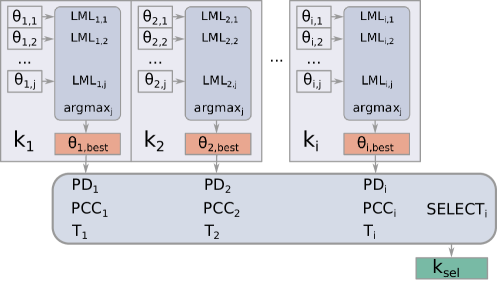
Figure 1: Two nested search procedures: The selection of the best hyperparameters for each kernel is made according to LML and the selection of the best kernel according to the BIC.

In this paper, the hyperparameters are optimized by means of Powell’s local search algorithm [25]. As this algorithm is not bounded, the search space has to be constrained by penalizing non-feasible hyperparameter sets. On the other hand, as the function to optimize might be multi-modal, a multi-start approach was used, performing a random restart every time the stopping criteria of the Powell’s algorithm are met, and getting the best overall result. During this hyperparameter search, a maximum number of $150$ evaluations of the LML were allowed.

Once the hyperparameters were optimized, in order to obtain the fitness of each kernel, PCC and the NLPD were evaluated by dividing the training set into 3 cross-validation folds. The results in each fold were averaged to obtain the actual fitness of each kernel. Finally, the time spent measuring both metrics in each fold was summed as a third objective.

Note that, as a result of the inclusion of the randomized restarts, the hyperparameters found for a certain kernel in two independent evaluations may not be the same. In fact, this implies that the fitness function optimized by the GP algorithm is stochastic.

5 Related work

Word embeddings [26] are extensively applied to NLP tasks [27]. The usual approach when combining embeddings from words in a sentence is to compute the average. This is the procedure used in [3], where 100-dimensional Glove embeddings [28] are the representation of choice for mapping texts to emotion scores using GaussProc regression.

GaussProcs are particularly suited to model uncertainty in the predictions and allow to accurately predict under noisy conditions. As such, there are diverse scenarios in which GaussProc can be applied to NLP tasks [29]. In all these problems the kernel function was selected beforehand, although its choice varies depending on the problem. The most frequently used kernel is the RBF kernel. However, this kernel is not suitable for all the problems. In [9], text periodicities of tweets are modeled using GaussProc with kernels specifically suited to capture the periodicities of the tweets. In the same paper, the periodic kernel (PER) and the periodic spike (PS) are shown to outperform non-periodic kernels and capture different periodic patterns. In [3], where GaussProcs are applied to SA, four different kernels are compared: SE, Linear, two Matern kernels. The Matern kernels are reported to produce better results than SE. In addition to numerical kernels, structural-kernels (e.g., tree-kernels) have been also combined with GaussProc.

Research on the evolution of kernel functions using evolutionary algorithms have shown that it is also possible to explore the space of kernel functions beyond the hyperparameter optimization. In the GaussProc literature this has been done by combining known kernels [30, 31, 32]. Kernels have also been evolved for Support Vector Machines (SVMs) [33, 34, 35, 36, 37, 38] and Relevance Vector Machines (RVMs) [39]. Some of the SVM approaches are also based in combining the well-known kernels [36, 37], although in some other works the kernels are learned from simple mathematical expressions [33, 34, 35, 38].

The particular characteristics determined by the GaussProcs make the evolution of kernels in this domain different to those algorithms used for SVMs and RVMs. Our approach considers different ways to evaluate the kernels based on a multi-objective approach, and creates kernels for GaussProc from scratch, without seeding components of human-designed kernels. This characteristic allows us to derive kernels that are not constrained by the prior knowledge while at the same time being optimized for the desired objectives.

6 Experiments

The goal of our experiments is to evaluate the performance of the introduced algorithm for the task of sentiment prediction from text. First we introduce the problem benchmark and word embeddings to evaluate the algorithm. Then, we describe the parameters used by the algorithms and explain the characteristics of the experimental framework, including the metrics used to compare the algorithms. Finally, we present the numerical results obtained from the experiments and discuss these results.

6.1 Problem benchmark and word-embeddings

We use the SemEval2007 Affective Text shared task dataset [19], following the work done in [3]. In this dataset, news headlines were manually annotated by experts, assigning to each text a degree of presence for each six Eckman [40] emotions: anger, disgust, fear, joy, sadness and surprise. In the original work, where this dataset was introduced, texts were divided into "dev" and "test" datasets. For the experiments presented in [3], the two sets were combined and further divided into $10$ folds used for cross-validation. We use this 10-fold partition to evaluate our algorithms.

In order to compute a representation for each text, punctuations in each headline were removed, tokenized [41], and case ignored. From the resulted text, the word-vector representation of each word were obtained using the 100-dimensional GloVe embeddings [28]. After deleting the words that were not found in the embedding, the representation of each headline was computed as the average of the words.

6.2 Experimental setup

Our experiments consists of learning a kernel for a GP regressor that predicts a particular emotion based on sentence embeddings. We evaluate the quality of the final kernels in terms of the PCC and NLPD metrics.

We compare MOECov algorithm with different variants of a-priori defined kernel methods, which were shown in [3] to produce good prediction results for the six emotions previously described. The kernels are presented in Table 1.

The parameters used by the evolutionary algorithm were:

• Population size: $N=38$,

• Number of generations: $G=65$,

• $O=2$,

• Mutation ($p_{m}=0.4$) and crossover ($p_{cx}=0.6$) probabilities,

• $\mu=9$,

• $\beta=1\mathrm{e}{-5}$

All algorithms were coded in Python. The implementation of MOECov is based on the EA software DEAP [42].

Due to the stochastic nature of the algorithm, for all algorithms and in every dataset, the kernel search process was repeated $30$ times along $10$ random cross-validation folds.

6.3 Results of the comparison between the algorithms

Table 2 shows the average PCC metric of the best solution obtained by the algorithms in the $30$ experiments. We remark that, these values have been computed on the test data, which we have not used for learning the GP programs. The results, for the NLPD metrics are shown in Table 3. In the tables, the best average value obtained for each of the sentiments are highlighted.

The analysis of the tables reveals that, in terms of the average fitness, MOECov improves all other kernels for both metrics in most of the cases. For the PCC metric, only in the disgust dataset, MOECov was not able to outperform the M52 kernel. For the NLPD metric, MOECov outperforms all the algorithms for all the sentiments.

Among the well-known kernels, M52 seems a better choice than the others, as it gets the second best result in average in the rest of the problems according to the PCC metric. M52 is also the second best choice in NLPD, only surpassed by SE kernel in the fear dataset, while the results of M32 and SE kernels are similar. As it can be appreciated in the tables, the LIN kernel is the worst performing kernel according to the average results.

	LIN	M32	M52	SE	MOECov
anger	0.58592	0.63556	0.6401	0.62629	0.64690
disgust	0.44828	0.52492	0.52782	0.50111	0.52456
fear	0.68056	0.728096	0.73059	0.72737	0.73555
joy	0.53832	0.55775	0.57459	0.56341	0.59158
sadness	0.63625	0.67148	0.68205	0.67876	0.69710
surprise	0.40311	0.45416	0.45647	0.43758	0.46751

Table 2: Mean results for PCC metric. Best results are shown in bold.

	LIN	M32	M52	SE	MOECov
anger	3.94141	3.92037	3.91162	3.93041	3.91084
disgust	3.81476	3.78148	3.77491	3.80068	3.77419
fear	4.16636	4.10615	4.1006	4.0986	4.07623
joy	4.34633	4.32588	4.30362	4.32737	4.29549
sadness	4.31082	4.28845	4.27618	4.28176	4.24454
surprise	4.06292	4.04524	4.04519	4.0511	4.02712

Table 3: Mean results for NLPD metric. Best results are shown in bold.

We conducted a statistical test to assess the existence of significant differences among the algorithms. For each metric and emotion, we applied the Friedman’s test [43] and we found significant differences in every comparison (p-values can be seen in the figures). Then, for each configuration, we applied a post-hoc test based on Friedman’s test, and adjusted its results with the Shaffer’s correction [44].

The results are shown in Figure 2 and Figure 3. The results confirm a coherent pattern where MOECov is the best performing algorithm for most of the datasets. However, it is also appreciated that according to this test, for most of the datasets, the differences between MOECov and M52 are not significant. In evaluating these results it is important to take into account that the kernels produced by MOECov have been generated completely from scratch, with no prior knowledge of the existing kernels. The algorithm is able evolve a well performing kernel starting from elementary mathematical components.

(a) Anger

(b) Disgust

(c) Fear

(d) Joy

(e) Sadness

(f) Surprise

Figure 2: Critical difference diagrams for the PCC metric. The kernels are ordered following the results in their ranking. The metrics with no significant differences between them are matched with a straight line.

(a) Anger

(b) Disgust

(c) Fear

(d) Joy

(e) Sadness

(f) Surprise

Figure 3: Critical difference diagrams for the NLPD metric. The kernel are ordered following the results in their ranking. The metrics with no significant differences between them are matched with a straight line.

6.4 Analysis of the MOECov evolution

One characteristic feature of our approach is that we simultaneously optimize different characteristics of the kernels. In order to determine whether the multi-objective approach effectively leads to the creation of more efficient kernels, both in terms of the accuracy for the prediction task, and in terms of efficiency, we analyze the fitness distribution of the solutions in the first and last population of MOECov for the anger dataset. These results are shown in Figure 4 where, in order to ease the visualization, results are shown for only one execution of the algorithm.

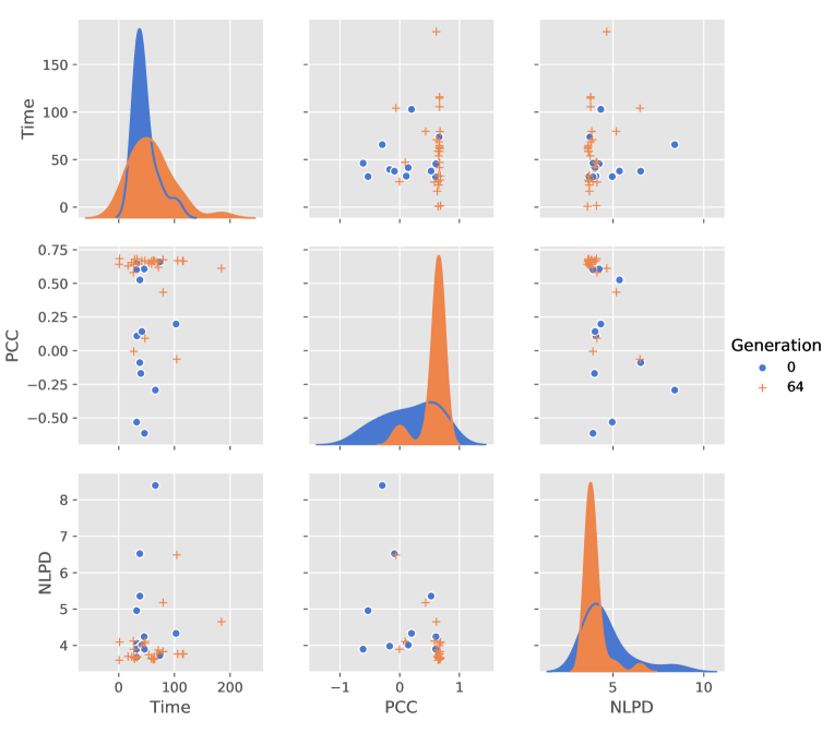
Figure 4: Distribution of the objective values in the first and last population of MOECov for one execution of the algorithm in the anger dataset.

In Figure 4 we represent the scatter plots for each possible pair of objectives. As it can be appreciated in the figures, from the first to the last population there is an improvement in the values of the objective values for the PCC and NLPD metrics. However, the computational time actually increases from the first to the last population. This result is not surprising since it is expected that the increase in accuracy of the trees is achieved by also augmenting their complexity. In this scenario we expect that using the time as a third objective can serve to counteract useless complexity gain of the programs, but the average time for learning the kernels will necessarily increase.

6.5 Transferability of the evolved kernels

An important question to analyze is whether the kernels evolved by MOECov are only valid for the sentiment datasets in which they have been learned or they can also be used to predict sentiment in the other datasets. This question can be frame on the general research that investigate the transferability of solutions found by evolutionary algorithms [45, 46, 47]. In order to answer this question, we have used the best programs learned for the anger dataset to make predictions in the other datasets. This can be considered as a transfer learning scenario in which the anger dataset is the source domain and all the other datasets serve as target domains. Notice, that in this particular example we do not recompute the hyperparameter values for the kernels. We simply apply the kernels as they are to the target datasets.

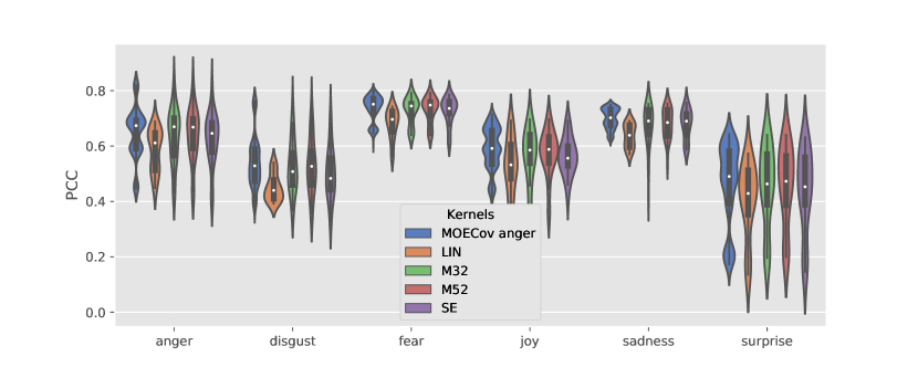
Figure 5: Results of the transferability experiments for the PCC metric. Each coloured shape shows a kernel density estimation of the distribution. A boxplot of the results is shown inside. More is better.

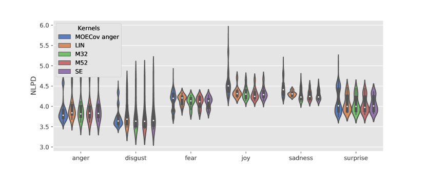
Figure 6: Results of the transferability experiments for the NLPD metric. Similar to the previous figure, a boxplot is shown inside each coloured shape that shows the estimation of the distribution. Less is better.

Figure 5 and Figure 6 respectively show the distributions of the objectives values obtained of this experiment for the PCC and NLPD metrics. In the figures, MOECov_anger indicates the kernels learned using the anger dataset. Notice that all the other algorithms have been learned using (training) data for each target dataset. The analysis of the figures indicate that the transferability of the kernels depends on the type of metric used. Results for PCC are at least as good as those obtained with the other kernels. However, for the NLPD metric results are slightly worse.

The main conclusion from this experiments is that the kernels evolved for predicting some sentiment can be also useful to predict other sentiments. This means that the embeddings contain the relevant information for the prediction and that the type of transformations that make a kernel a good predictor are similar across sentiment domains.

7 Conclusions

Sentiment classification is a relevant problem in NLP. In previous work it has been shown that GaussProc regression is an efficient approach to solve this problem when considering predicting the sentiment with a finer level of detail, as a regression problem. However, our hypothesis was that the fixed structure used by classical kernels lacks the flexibility to capture more subtle differences in datasets. Therefore, in this paper we have proposed MOECov as way to evolve the structure of the kernels. By addressing the creation of kernels as a multi-objective problem we have been able to generate kernels that simultaneously optimize two of the accuracy metrics previously proposed, and in addition are optimized for computational complexity.

As far as the authors are concerned this is the first work that uses evolved GaussProcs for NLP problems. We had not found either previous studies that tries to optimize the hyper-parameters of fixed kernels simultaneously considering two or more metrics.

There are a number of ways in which our studied could be extended. Other sentiment datasets, possibly in other languages, could be considered. Furthermore, other semantic classification tasks, such as, the post-editing effort prediction could be addressed using our approach. We also noticed that at the time of stopping the MOECov algorithm the quality of the solutions was still improving. Therefore, more fitness evaluations are likely to produce better results of the algorithm. Furthermore, automatic tuning of the algorithm’s parameters should be accomplished since we did not tune the parameters of the algorithm for the present study.

References

- [1] Jan Deriu, Aurelien Lucchi, Valeria De Luca, Aliaksei Severyn, Simon Müller, Mark Cieliebak, Thomas Hofmann, and Martin Jaggi. Leveraging Large Amounts of Weakly Supervised Data for Multi-Language Sentiment Classification. In Proceedings of the 26th International Conference on World Wide Web, WWW ’17, pages 1045–1052, Republic and Canton of Geneva, Switzerland, 2017. International World Wide Web Conferences Steering Committee. event-place: Perth, Australia.
- [2] Richard Socher, Jeffrey Pennington, Eric H. Huang, Andrew Y. Ng, and Christopher D. Manning. Semi-supervised Recursive Autoencoders for Predicting Sentiment Distributions. In Proceedings of the Conference on Empirical Methods in Natural Language Processing, EMNLP ’11, pages 151–161, Stroudsburg, PA, USA, 2011. Association for Computational Linguistics. event-place: Edinburgh, United Kingdom.
- [3] Daniel Beck. Modelling Representation Noise in Emotion Analysis using Gaussian Processes. In Proceedings of the Eighth International Joint Conference on Natural Language Processing (Volume 2: Short Papers), pages 140–145, Taipei, Taiwan, November 2017. Asian Federation of Natural Language Processing.
- [4] Daniel Beck, Trevor Cohn, Christian Hardmeier, and Lucia Specia. Learning Structural Kernels for Natural Language Processing. Transactions of the Association for Computational Linguistics, 3:461–473, December 2015.
- [5] Daniel Beck and Trevor Cohn. Learning Kernels over Strings using Gaussian Processes. In Proceedings of the Eighth International Joint Conference on Natural Language Processing (Volume 2: Short Papers), pages 67–73, Taipei, Taiwan, November 2017. Asian Federation of Natural Language Processing.
- [6] Daniel Emilio Beck. Gaussian Processes for Text Regression. phd, University of Sheffield, June 2017.
- [7] C. E. Rasmussen and C. K. Williams. Gaussian processes for machine learning. MIT Press, 2006.
- [8] Tamara Polajnar, Simon Rogers, and Mark Girolami. Protein interaction detection in sentences via Gaussian Processes: a preliminary evaluation. International journal of data mining and bioinformatics, 5(1):52–72, 2011.
- [9] Daniel Preoţiuc-Pietro and Trevor Cohn. A temporal model of text periodicities using Gaussian Processes. In Proceedings of the 2013 Conference on Empirical Methods in Natural Language Processing, pages 977–988, 2013.
- [10] Trevor Cohn and Lucia Specia. Modelling annotator bias with multi-task gaussian processes: An application to machine translation quality estimation. In Proceedings of the 51st Annual Meeting of the Association for Computational Linguistics (Volume 1: Long Papers), volume 1, pages 32–42, 2013.
- [11] Kashif Shah, Trevor Cohn, and Lucia Specia. An investigation on the effectiveness of features for translation quality estimation. In Proceedings of the Machine Translation Summit, volume 14, pages 167–174. Citeseer, 2013.
- [12] David Duvenaud. Automatic model construction with Gaussian processes. Thesis, University of Cambridge, 2014.
- [13] Marc G. Genton. Classes of Kernels for Machine Learning: A Statistics Perspective. J. Mach. Learn. Res., 2:299–312, March 2002.
- [14] Manuel Blum and Martin Riedmiller. Optimization of Gaussian Process Hyperparameters using Rprop. In European Symposium on Artificial Neural Networks, Computational Intelligence and Machine Learning, 2013.
- [15] Karl Pearson. Note on regression and inheritance in the case of two parents. Proceedings of the Royal Society of London, 58:240–242, 1895.
- [16] Joaquin Quiñonero-Candela, Carl Edward Rasmussen, Fabian Sinz, Olivier Bousquet, and Bernhard Schölkopf. Evaluating Predictive Uncertainty Challenge. In Joaquin Quiñonero-Candela, Ido Dagan, Bernardo Magnini, and Florence d’Alché Buc, editors, Machine Learning Challenges. Evaluating Predictive Uncertainty, Visual Object Classification, and Recognising Tectual Entailment, Lecture Notes in Computer Science, pages 1–27. Springer Berlin Heidelberg, 2006.
- [17] John R. Koza. Genetic Programming: On the Programming of Computers by Means of Natural Selection. MIT Press, 1992.
- [18] Bo Pang and Lillian Lee. Opinion Mining and Sentiment Analysis. Foundations and Trends® in Information Retrieval, 2(1–2):1–135, July 2008.
- [19] Carlo Strapparava and Rada Mihalcea. SemEval-2007 Task 14: Affective Text. In Proceedings of the 4th International Workshop on Semantic Evaluations, SemEval ’07, pages 70–74, Stroudsburg, PA, USA, 2007. Association for Computational Linguistics.
- [20] Tomas Mikolov, Kai Chen, Greg Corrado, and Jeffrey Dean. Efficient Estimation of Word Representations in Vector Space. arXiv:1301.3781 [cs], January 2013. arXiv: 1301.3781.
- [21] J. Mercer and B. A. XVI. Functions of positive and negative type, and their connection the theory of integral equations. Phil. Trans. R. Soc. Lond. A, 209(441-458):415–446, January 1909.
- [22] Lucia Specia. Exploiting objective annotations for measuring translation post-editing effort. In Proceedings of the 15th Conference of the European Association for Machine Translation, pages 73–80, 2011.
- [23] David J. Montana. Strongly Typed Genetic Programming. Evolutionary Computation, 3(2):199–230, June 1995.
- [24] Kalyanmoy Deb, Samir Agrawal, Amrit Pratap, and T. Meyarivan. A Fast Elitist Non-dominated Sorting Genetic Algorithm for Multi-objective Optimization: NSGA-II. In Marc Schoenauer, Kalyanmoy Deb, Günther Rudolph, Xin Yao, Evelyne Lutton, Juan Julian Merelo, and Hans-Paul Schwefel, editors, Parallel Problem Solving from Nature PPSN VI, Lecture Notes in Computer Science, pages 849–858. Springer Berlin Heidelberg, 2000.
- [25] M. J. D. Powell. An efficient method for finding the minimum of a function of several variables without calculating derivatives. The Computer Journal, 7(2):155–162, January 1964.
- [26] Tomas Mikolov, Ilya Sutskever, Kai Chen, Greg S Corrado, and Jeff Dean. Distributed Representations of Words and Phrases and their Compositionality. In C. J. C. Burges, L. Bottou, M. Welling, Z. Ghahramani, and K. Q. Weinberger, editors, Advances in Neural Information Processing Systems 26, pages 3111–3119. Curran Associates, Inc., 2013.
- [27] Vasileios Lampos, Bin Zou, and Ingemar Johansson Cox. Enhancing Feature Selection Using Word Embeddings: The Case of Flu Surveillance. In Proceedings of the 26th International Conference on World Wide Web, WWW ’17, pages 695–704, Republic and Canton of Geneva, Switzerland, 2017. International World Wide Web Conferences Steering Committee. event-place: Perth, Australia.
- [28] Jeffrey Pennington, Richard Socher, and Christopher Manning. Glove: Global vectors for word representation. In Proceedings of the 2014 conference on empirical methods in natural language processing (EMNLP), pages 1532–1543, 2014.
- [29] Trevor Cohn, Daniel Preotiuc-Pietro, and Neil Lawrence. Gaussian processes for natural language processing. In Proceedings of the 52nd Annual Meeting of the Association for Computational Linguistics: Tutorials, pages 1–3, 2014.
- [30] Gabriel Kronberger and Michael Kommenda. Evolution of Covariance Functions for Gaussian Process Regression Using Genetic Programming. In Computer Aided Systems Theory - EUROCAST 2013, Lecture Notes in Computer Science, pages 308–315. Springer, Berlin, Heidelberg, February 2013.
- [31] David Duvenaud, James Lloyd, Roger Grosse, Joshua Tenenbaum, and Ghahramani Zoubin. Structure Discovery in Nonparametric Regression through Compositional Kernel Search. In Proceedings of The 30th International Conference on Machine Learning, pages 1166–1174, 2013.
- [32] James Robert Lloyd, David Duvenaud, Roger Grosse, Joshua Tenenbaum, and Zoubin Ghahramani. Automatic Construction and Natural-Language Description of Nonparametric Regression Models. In Twenty-Eighth AAAI Conference on Artificial Intelligence, June 2014.
- [33] Tom Howley and Michael G. Madden. An Evolutionary Approach to Automatic Kernel Construction. In Artificial Neural Networks – ICANN 2006, Lecture Notes in Computer Science, pages 417–426. Springer, Berlin, Heidelberg, September 2006.
- [34] Christian Gagné, Marc Schoenauer, Michèle Sebag, and Marco Tomassini. Genetic Programming for Kernel-Based Learning with Co-evolving Subsets Selection. In Parallel Problem Solving from Nature - PPSN IX, Lecture Notes in Computer Science, pages 1008–1017. Springer, Berlin, Heidelberg, 2006.
- [35] L. Diosan, A. Rogozan, and J. P. Pecuchet. Evolving kernel functions for SVMs by genetic programming. In Sixth International Conference on Machine Learning and Applications (ICMLA 2007), pages 19–24, 2007.
- [36] Keith M. Sullivan and Sean Luke. Evolving Kernels for Support Vector Machine Classification. In Proceedings of the 9th Annual Conference on Genetic and Evolutionary Computation, GECCO ’07, pages 1702–1707, New York, NY, USA, 2007. ACM.
- [37] Laura Dioşan, Alexandrina Rogozan, and Jean-Pierre Pecuchet. Improving classification performance of Support Vector Machine by genetically optimising kernel shape and hyper-parameters. Applied Intelligence, 36(2):280–294, March 2012.
- [38] Patrick Koch, Bernd Bischl, Oliver Flasch, Thomas Bartz-Beielstein, Claus Weihs, and Wolfgang Konen. Tuning and evolution of support vector kernels. Evolutionary Intelligence, 5(3):153–170, September 2012.
- [39] Wu Bing, Zhang Wen-qiong, Chen Ling, and Liang Jia-hong. A GP-based kernel construction and optimization method for RVM. In 2010 The 2nd International Conference on Computer and Automation Engineering (ICCAE), volume 4, pages 419–423, February 2010.
- [40] Paul Ekman. Facial expression and emotion. American psychologist, 48(4):384, 1993.
- [41] Steven Bird, Ewan Klein, and Edward Loper. Natural language processing with Python: analyzing text with the natural language toolkit. " O’Reilly Media, Inc.", 2009.
- [42] Félix-Antoine Fortin, François-Michel De Rainville, Marc-André Gardner, Marc Parizeau, and Christian Gagné. DEAP: Evolutionary Algorithms Made Easy. Journal of Machine Learning Research, 13(Jul):2171–2175, 2012.
- [43] Milton Friedman. The use of ranks to avoid the assumption of normality implicit in the analysis of variance. Journal of the american statistical association, 32(200):675–701, 1937.
- [44] Juliet Popper Shaffer. Modified Sequentially Rejective Multiple Test Procedures. Journal of the American Statistical Association, March 2012.
- [45] M. Iqbal, M. Zhang, and B. Xue. Improving classification on images by extracting and transferring knowledge in genetic programming. In 2016 IEEE Congress on Evolutionary Computation (CEC), pages 3582–3589, July 2016.
- [46] Unai Garciarena, Roberto Santana, and Alexander Mendiburu. Evolved GANs for Generating Pareto Set Approximations. In Proceedings of the Genetic and Evolutionary Computation Conference, GECCO ’18, pages 434–441, New York, NY, USA, 2018. ACM. event-place: Kyoto, Japan.
- [47] R. Santana, A. Mendiburu, and J. A. Lozano. Structural transfer using EDAs: An application to multi-marker tagging SNP selection. In 2012 IEEE Congress on Evolutionary Computation, pages 1–8, June 2012.