An all-electron product-basis set: application to plasmon anisotropy in simple metals

Abstract

An efficient basis set for products of all-electron wave functions is proposed, which comprises plane waves defined over the entire unit cell and orbitals confined to small non-overlapping spheres. The size of the set and the basis functions are, in principle, independent of the computational parameters of the band structure method. The approach is implemented in the extended LAPW method, and its properties and accuracy are discussed. The method is applied to analyze the dielectric response of the simple metals Al, Na, Li, K, Rb, and Cs with a focus on the origin of the anisotropy of the plasmon dispersion in Al and Na. The anisotropy is traced to tiny structures of the one-particle excitation spectra of Al and Na, and relevant experimental observations are explained.

I Introduction

The microscopic dielectric function (DF) $\epsilon(\mathbf{r},\mathbf{r}^{\prime};\omega)$ is a key ingredient in the theory of the ground state Giuliani and Vignale (2005), quasiparticles Hedin (1965); Aryasetiawan and Gunnarsson (1998), optical Haug and Koch (2004) and plasmonic Pines (1963); Feibelman (1982); Liebsch (1997); Pitarke et al. (2007) excitations as well as in the electron spectroscopies where the microscopic electric field in the solid is a crucial aspect: photoemission at low photon energies Krasovskii et al. (2010), laser-assisted time-resolved spectroscopy Siek et al. (2017), or the theory of energy losses by quantum particles Nazarov et al. (2017). The variety of applications and the growing demand for a detailed description of the DF calls for the development of an efficient basis set to express the relevant operators in order to facilitate ab initio calculations of the DF.

A general and rigorous analysis of the basis set problem was presented by Harriman Harriman (1986), and various practical schemes have been implemented. The simplest case are pseudopotential methods Payne et al. (1992); Blöchl (1994), where the plane-wave (PW) basis for the Bloch wave functions $\psi^{\mathbf{k}}_{\lambda}$ is ideally suited for the Fourier representation of the dielectric matrix $\epsilon_{\mathbf{G}\mathbf{G}^{\prime}}(\mathbf{q},\omega)$, which immediately follows from the Fourier expansion of the products $\psi^{\mathbf{k}*}_{\lambda^{\prime}}\psi^{\mathbf{k}-\mathbf{q}}_{\lambda}$. Furthermore, the accuracy of both $\psi^{\mathbf{k}}_{\lambda}$ and $\epsilon(\mathbf{r},\mathbf{r}^{\prime};\omega)$ is consistently controlled by a cutoff in the reciprocal space. Another obvious choice is a real-space grid Brodersen et al. (2002); Mortensen et al. (2005), however, the experience with the projected augmented wave method shows that atomic-orbital basis is computationally more efficient Yan et al. (2011). Typical implementation of the orbital basis in the context of pseudopotentials and accompanying approximations are discussed in Refs. Blase and Ordejón, 2004; Umari et al., 2009. The problem becomes nontrivial in all-electron methods, where the basis functions have complicated shape, and their products are unwieldy. In addition, the resulting product set is non-orthogonal and overcomplete, and there is no a priori criterion to reduce the set and to control its convergence. For orbital basis sets, methods of numerical elimination of redundant products were suggested by Aryasetiawan and Gunnarsson Aryasetiawan and Gunnarsson (1994) for muffin-tin orbitals and by Foerster Foerster (2008) for atomic orbitals. The most accurate wave functions are provided by the augmented plane wave (APW) formalism, where the basis functions are still more complicated Slater (1937); Andersen (1975); Koelling and Arbman (1975); Singh (1991); Krasovskii (1997). In the LAPW-based (linear APW) codes Jiang et al. (2013); Friedrich et al. (2010); Nabok et al. (2016), criteria similar to those of Refs. Aryasetiawan and Gunnarsson, 1994; Foerster, 2008 are applied to obtain a reduced set from the products of APWs. However, no attempt has been made to construct a universal basis to parametrize the products.

Here, we propose a basis set to calculate the $\epsilon$ matrix out of all-electron wave functions, which is suitable for (but not limited to) the APW representation. The product basis set consists of plane waves that are defined throughout the unit cell (not just in the interstitial region, in contrast to Refs. Jiang et al., 2013; Kotani and van Schilfgaarde, 2002; Friedrich et al., 2010, 2011; Nabok et al., 2016) and orbitals centered at atomic sites and confined to small non-overlapping spheres. We refer to the latter as island orbitals (IOs) to distinguish them from the localized orbitals (LOs) of the extended LAPW methods Singh (1991); Krasovskii (1997). The basis functions are derived from an approximation to the all-electron wave functions, which also has the PW+IO structure, and whose accuracy is regulated by the angular-momentum cutoff of the orbital part and by the $|\mathbf{k}+\mathbf{G}|$ cutoff of the plane wave part. Owing to the orthogonality of the plane waves and to the finite domain of the orbitals, the basis set provides an efficient scheme for the matrix elements $\langle\,\mathbf{k}+\mathbf{q}\lambda^{\prime}\,|\,\exp[i(\mathbf{q}+\mathbf{G})\cdot\mathbf{r}]\,|\,\mathbf{k}\lambda\,\rangle$. Thus, the Fourier representation $\epsilon_{\mathbf{G}\mathbf{G}^{\prime}}(\mathbf{q},\omega)$ is readily obtained, which is convenient, in particular because the Coulomb interaction becomes diagonal and because the reciprocal lattice vector $\mathbf{G}$ is a natural cutoff parameter to systematically refine the accuracy of the DF.

To demonstrate the viability of the method we address the $\mathbf{q}$-dependent longitudinal DF of simple metals, focusing on the anisotropy of the plasmon dispersion. We analyze the similarities and differences in the anisotropy scenarios in Al and Na and explain the experimentally long-known opposite behavior of the anisotropy of the Drude plasmon relative to the low-energy zone boundary collective state (ZBCS) Foo and Hopfield (1968) in the two metals. Further, we compare Al and Na with the less free-electron-like alkali metals Li, K, Rb, and Cs.

The paper is organized as follows. In the next section we describe the PW+IO representation of the wave functions and the resulting formalism for the DF. The accuracy and convergence of the product basis are analyzed in Appendix. Computational aspects not related to the new method are presented in Sec. III. In Sec. IV, plasmon dispersion in aluminum and alkali metals is discussed.

II formalism

Of all the band structure methods, the formalism of augmented plane waves introduced by Slater Slater (1937) has the least limitations regarding the accuracy of the wave functions. Here, we consider an implementation for a basis of energy-independent APWs Andersen (1975); Koelling and Arbman (1975) extended by localized orbitals Singh (1991); Krasovskii (1997).

II.1 Filtering the all-electron wave function

The wave function $\psi_{\lambda}^{\mathbf{k}}$ for the Bloch vector $\mathbf{k}$ and band number $\lambda$ is a sum of $N_{\xi}$ APWs $\xi(\mathbf{r})$ and $N_{\zeta}$ localized orbitals $\zeta(\mathbf{r})$. For one atom per unit cell located at $\mathbf{r}=0$ it reads

$$\psi_{\lambda}^{\mathbf{k}}(\mathbf{r})=\sum_{\mathbf{G}}^{N_{\xi}}p_{\mathbf{G}}^{\lambda\mathbf{k}}\xi_{\mathbf{G}}^{\mathbf{k}}(\mathbf{r})+\sum_{lm}\sum_{\nu}^{\bar{\nu}_{l}}q_{\nu lm}^{\lambda\mathbf{k}}\zeta_{l\nu}(r)Y_{lm}(\mathbf{\hat{r}}).$$ (1)

Here $p$ and $q$ comprise the set of variational coefficients, $p$ being coefficients of the APWs and $q$ of the LOs, and $\mathbf{G}$ are reciprocal lattice vectors. The APW $\xi_{\mathbf{G}}^{\mathbf{k}}$ is smoothly continuous everywhere in the unit cell, and outside the muffin-tin (MT) spheres it coincides with the plane wave $\exp[i(\mathbf{k}+\mathbf{G})\cdot\mathbf{r}]$. The LOs vanish with their radial derivatives at the muffin-tin sphere and remain zero in the interstitial region. Subscript $\nu$ indicates the radial part of the local orbital, so $N_{\zeta}=\sum_{l}\bar{\nu}_{l}(2l+1)$.

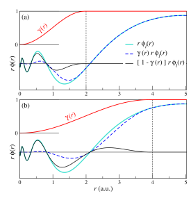
Figure 1: $\gamma$-partitioning in the sphere of Cs for $S_{\gamma}=2$ a.u. (a) and $S_{\gamma}=4$ a.u. (b): radial solution (thick light-blue line) is multiplied by $\gamma(r)$ (thick red line). The gouging radii $S_{\gamma}$ are indicated by vertical dashed lines, MT radius is 5.02 a.u. The radial function is for $l=0$, and energy is at the Fermi level.

In the sphere the angular-momentum expansion of the APW of a wave vector $\mathbf{K}=\mathbf{k}+\mathbf{G}$ reads

$$\xi_{\mathbf{G}}^{\mathbf{k}}(\mathbf{r})=\sum_{lm}[\,A_{lm}(\mathbf{K})\phi_{l}(r)+B_{lm}(\mathbf{K})\dot{\phi}_{l}(r)\,]\,Y_{lm}(\mathbf{\mathbf{\hat{r}}}),$$ (2)

where $\phi_{l}$ is a solution of the radial Schrödinger equation and $\dot{\phi}_{l}$ is its energy derivative Andersen (1975); Koelling and Arbman (1975). Coefficients $A_{lm}$ and $B_{lm}$ are determined from the condition that the APW be smoothly continuous at the sphere boundary, $r=S$. Thus, for each $l$ the radial basis comprises $\bar{n}_{l}=\bar{\nu}_{l}+2$ functions $u_{ln}$, where $u_{l1}=\phi_{l}$, $u_{l2}=\dot{\phi}_{l}$, and the radial part of the LO is a linear combination of three functions: $\zeta_{l\nu}=u_{l(\nu+2)}+a_{l\nu}\phi_{l}+b_{l\nu}\dot{\phi}_{l}$. Usually, $u_{l(\nu+2)}$ are also radial solutions for different energies, although in some applications they may be more complicated functions Krasovskii and Schattke (2001); Michalicek et al. (2013).

A straightforwardly constructed set of products of $N=N_{\xi}+N_{\zeta}$ functions would comprise $N(N+1)/2$ terms, of which a much smaller number are linearly independent and physically relevant. There is no universal recipe to a priori select the optimal subset—without reference to the specific shape of the APWs—although some intuitive criteria and practical schemes were suggested in Refs. Aryasetiawan and Gunnarsson, 1994; Jiang et al., 2013. Here we develop an approach that avoids an explicit construction of the products of the APWs, but instead employs an approximate (filtered) representation of the wave functions to generate the product basis. This approximate representation has the property that both the accuracy of the filtered wave functions and the completeness of the product basis are naturally controlled by a spatial resolution criterion, i.e., by the $\mathbf{G}$-vector cutoff of the PW set and by the $lm$-cutoff of the IO set.

To arrive at the optimal partitioning between the PW and IO components of the filtered wave function, we first modify the original wave function $\psi$ by damping its rapid oscillations in the vicinity of the nuclei: within a sphere of radius $S_{\gamma}$ (smaller than the muffin-tin radius, see Fig. 1) we multiply $\psi$ by a function $\gamma(r)$ that is zero at $r=0$ and steadily grows to reach unity at $r=S_{\gamma}$:

$$\gamma(r)=\left\{\begin{array}[]{ll}\dfrac{1}{2}\left(1-\cos\dfrac{\pi r}{S_{\gamma}}\right)&\text{for}\leavevmode\nobreak\ r\leq S_{\gamma},\\ 1&\text{for}\leavevmode\nobreak\ r>S_{\gamma}.\\ \end{array}\right.$$ (5)

The gouged function $\gamma\psi$ has a rapidly convergent plane-wave expansion Krasovskii et al. (1999); Krasovskii and Schattke (1999), which constitutes the Fourier part $\psi^{\text{F}}$ of the filtered wave function:

$$\psi=\gamma\psi+(1-\gamma)\psi\approx\psi^{\text{F}}+(1-\gamma)\psi\approx\psi^{\text{F}}+\psi^{\text{I}}.$$ (6)

Here $\psi^{\text{I}}$ is an approximation to $(1-\gamma)\psi$ obtained by truncating the angular-momentum expansion of $\psi$. It consists of isolated islands around the nuclei, and the smaller the radius $S_{\gamma}$ of the island the faster converges the $lm$ series of $\psi^{\text{I}}$ and the slower does the PW series of $\psi^{\text{F}}$. For sufficiently small $\gamma$ spheres, $\psi^{\text{I}}$ can be completely neglected to a good approximation Krasovskii and Schattke (1999); Krasovskii et al. (1999). In Appendix, we present a detailed study of the convergence and accuracy of the $\psi^{\text{F}}+\psi^{\text{I}}$ representation.

II.2 Density matrix elements

Let us consider the operator $\hat{o}=\exp(i\mathbf{q}\!\cdot\!\mathbf{r})$. Using the notation $\psi_{\lambda}=\left\langle\,\mathbf{r}\,|\,\psi_{\lambda}\,\right\rangle$, $\psi^{\text{F}}_{\lambda}=\left\langle\,\mathbf{r}\,|\,F_{\lambda}\,\right\rangle$, and $\psi^{\text{I}}_{\lambda}=\left\langle\,\mathbf{r}\,|\,I_{\lambda}\,\right\rangle$ for the approximate wave functions $\psi_{\lambda}=\psi^{\text{F}}_{\lambda}+\psi^{\text{I}}_{\lambda}$ given by Eq. (6) we write the matrix element $\langle\,\psi_{\lambda}\,|\,\hat{o}\,|\,\psi_{\mu}\,\rangle$ as a sum of an integral over the entire unit cell $\langle\,F_{\lambda}\,|\,\hat{o}\,|\,F_{\mu}\,\rangle$ and three integrals over the small $\gamma$-spheres:

$$\langle\,\psi_{\lambda}\,|\,\hat{o}\,|\,\psi_{\mu}\,\rangle = \langle\,F_{\lambda}\,|\,\hat{o}\,|\,F_{\mu}\,\rangle$$

$$+ \langle\,F_{\lambda}\,|\,\hat{o}\,|\,I_{\mu}\,\rangle+\langle\,I_{\lambda}\,|\,\hat{o}\,|\,F_{\mu}\,\rangle+\langle\,I_{\lambda}\,|\,\hat{o}\,|\,I_{\mu}\,\rangle.\quad$$

The first term in the right hand side is readily calculated via plane waves, and the integrals over the $\gamma$-spheres can be calculated in the angular-momentum representation in view of the relation $\psi^{\text{F}}\approx\gamma\psi$, see Eq. (6). Their sum reduces to $\langle\,\psi_{\lambda}\,|\,\hat{o}\,|\,\psi_{\mu}\,\rangle_{\gamma}-\langle\,F_{\lambda}\,|\,\hat{o}\,|\,F_{\mu}\,\rangle_{\gamma}$, where the subscript $\gamma$ indicates that the integration is limited to the $\gamma$-spheres. The computational efficiency of this scheme stems from the following properties: First, the $lm$ series converges fast because the $\gamma$-spheres are small, and it is helpful that the coefficients are the same for the wave function $\psi$ and for its Fourier-filtered part $\psi^{\text{F}}$. Second, the plane-wave expansion of $\gamma\psi$ contains a reasonable number of plane waves because—in contrast to the energy-eigenvalue problem—a high accuracy close to the nucleus is not needed (see Appendix). Note that the approximate function (6) is smoothly continuous by construction at any $l$-cutoff, whereas in the original APW representation one has to include rather high angular momenta to achieve the continuity. This property is important, in particular for the construction of the effective potentials from orbital-dependent functionals Betzinger et al. (2011) .

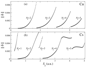
Figure 2: Accuracy of the representation of the radial density matrix $U_{ll^{\prime}nn^{\prime}}(r)$ by a reduced orthogonal basis set, see the last paragraph of Sec. II.2. The error $\|\,\delta(N_{\varepsilon},S_{\gamma})\,\|$ is shown for the products of the $d$-orbitals of Cu (a) and $p$-orbitals of Cs (b). The overlap eigenvalue cutoff is $\varepsilon=0.0001$.

The operator $\exp(i\mathbf{q}\cdot\mathbf{r})$ is diagonal in the PW basis, so the first term in Eq. (II.2) is easy to calculate. The contribution from the islands is obtained from the angular-momentum decomposition of the wave functions inside the muffin-tin spheres

$$\psi_{\lambda}^{\mathbf{k}}(\mathbf{r})=\sum_{l}^{l_{\text{max}}}\sum_{n}^{\bar{n}_{l}}\sum_{m=-l}^{l}C_{lnm}^{\mathbf{k}\lambda}u_{ln}(r)Y_{lm}(\mathbf{\hat{r}})$$ (8)

using the Rayleigh expansion of $\exp(i\mathbf{q}\!\cdot\!\mathbf{r})$:

$$\langle\,\psi_{\lambda^{\prime}}^{\mathbf{k}+\mathbf{q}}\,|\,e^{i\mathbf{q}\cdot\mathbf{r}}\,|\,\psi_{\lambda}^{\mathbf{k}}\,\rangle_{\gamma}-\langle\,F_{\lambda^{\prime}}^{\mathbf{k}+\mathbf{q}}\,|\,e^{i\mathbf{q}\cdot\mathbf{r}}\,|\,F_{\lambda}^{\mathbf{k}}\,\rangle_{\gamma}=\sum_{ll^{\prime}}^{l_{\text{max}}}\sum_{nn^{\prime}}\sum_{mm^{\prime}}\left[C^{\mathbf{k}+\mathbf{q}\lambda^{\prime}}_{l^{\prime}n^{\prime}m^{\prime}}\right]^{*}C^{\mathbf{k}\lambda}_{lnm}\sum_{l^{\prime\prime}}^{l^{\prime\prime}_{\text{max}}}T_{ll^{\prime}mm^{\prime}}^{l^{\prime\prime}}(\mathbf{\hat{q}})\int\limits_{0}^{S_{\gamma}}\!j_{l^{\prime\prime}}(qr)U_{ll^{\prime}nn^{\prime}}(r)\,dr,$$ (9)

where the angular integration yields

$$T_{ll^{\prime}mm^{\prime}}^{l^{\prime\prime}}(\mathbf{\hat{q}})={4\pi}i^{l^{\prime\prime}}Y^{*}_{l^{\prime\prime}m^{\prime\prime}}(\mathbf{\hat{q}})\int Y_{l^{\prime}m^{\prime}}^{*}Y_{l^{\prime\prime}m^{\prime\prime}}Y_{lm}\;d\mathbf{\mathbf{\hat{r}}}.$$ (10)

Here $lm$ and $l^{\prime}m^{\prime}$ refer to the angular-momentum decomposition of $\psi_{\lambda}^{\mathbf{k}}$ and $\psi_{\lambda^{\prime}}^{\mathbf{k}+\mathbf{q}}$, respectively, and $l^{\prime\prime}$ to the Rayleigh expansion of $\exp(i\mathbf{q}\!\cdot\!\mathbf{r})$. The radial functions

$$U_{ll^{\prime}nn^{\prime}}(r)=u_{l^{\prime}n^{\prime}}(r)u_{ln}(r)[1-\gamma(r)^{2}]r^{2}$$ (11)

are products of the radial parts of APWs multiplied by the confining function $[1-\gamma(r)^{2}]r^{2}$. Because the radii $S_{\gamma}$ are independent of the other computational parameters they can be chosen rather small, typically 1 to 2 a.u., so that the angular-momentum sums can be truncated at rather low $l$, as will be demonstrated in the next section. To summarize, the PW+IO product basis set consists of plane waves $\exp[i(\mathbf{q}+\mathbf{G})\cdot\mathbf{r}]$ and island orbitals $U_{ln}(r)Y_{lm}(\mathbf{\hat{r}})$ whose radial shape is given by Eq. (11) and angular part by Eq. (10). Its size scales linearly with the size of the unit cell, and the IO part can be further reduced by removing the linearly dependent IOs Aryasetiawan and Gunnarsson (1994); Foerster (2008); Friedrich et al. (2010); Jiang et al. (2013); Koval et al. (2014).

According to Eq. (11), for each pair of $l$ and $l^{\prime}$ the set of radial products comprises $\bar{n}_{l}\times\bar{n}_{l^{\prime}}$ functions, and large $\bar{n}_{l}$ may be needed to describe a wide energy interval. For example, in order to achieve convergence of the $GW$ method with respect to the number of unoccupied states it may be necessary to include up to $\bar{n}_{l}=8$ radial functions per $lm$-channel Friedrich et al. (2011); Nabok et al. (2016); Jiang (2018). A straightforward inclusion of all the products $u_{l^{\prime}n^{\prime}}u_{ln}$ may lead to an excessively large and linearly dependent basis set. Here, we can take advantage of the fact that $U_{ll^{\prime}nn^{\prime}}(r)$ are restricted to a close vicinity of the potential singularity, where the radial solutions change very slowly with energy Andersen (1975); Michalicek et al. (2013), so the number of physically relevant $u_{ln}$ is much smaller. Moreover, their shape is determined by the potential singularity, and it is practically independent of the crystal potential. Thus, for a given $S_{\gamma}$, the functions $U_{ll^{\prime}nn^{\prime}}(r)$ can be tabulated for each element.

To demonstrate how a relevant set can be selected out of a full set of functions $U_{ll^{\prime}nn^{\prime}}(r)$, let us take the MT sphere of Cu as an example and consider the contribution of the $d$-orbitals to the spherical part $l^{\prime\prime}=0$ of Eq. (9). The 3$d$ band is described by the radial solution at the energy $E=-3$ eV relative to the Fermi level and by its energy derivative. The radial set is extended by a 4$d$ and a 5$d$ function at $E=40$ and 133 eV, respectively. This gives rise to $N_{U}=10$ functions $U_{llnn^{\prime}}(r)$ with $l=2$. We now diagonalize the overlap matrix of the functions $U_{llnn^{\prime}}(r)$ and retain only the eigenvectors of eigenvalues larger than some predefined $\varepsilon$. The number $N_{\varepsilon}$ of the retained functions is the smaller the smaller the gouging radius $S_{\gamma}$. We then fit the $N_{U}$ original functions with the $N_{\varepsilon}$ orthogonal functions and in Fig. 2(a) present the maximal error $\|\,\delta(N_{\varepsilon},S_{\gamma})\,\|$ as a function of $S_{\gamma}$. Figure 2(b) shows the performance of the orthogonal set in the sphere of Cs for four $p$-orbitals comprising $\phi$ and $\dot{\phi}$ at the 5$p$ branch and two $\phi$ functions at the 6$p$ and 7$p$ branches. Thus, the accuracy with which the radial part of the product set is represented is flexibly adjusted by the gouging radius and by the number of the orthogonal basis functions.

The data on the accuracy of the product-set expansion regarding the number of PWs in $\psi^{\text{F}}$ and IOs in $\psi^{\text{I}}$, Eq. (6), as well as on the $l^{\prime\prime}$ convergence of the $\exp(i\mathbf{q}\!\cdot\!\mathbf{r})$ operator, Eq. (9), are given in Appendix. For sufficiently large $S_{\gamma}$ the number of PWs may be chosen comparable to the number of APWs, while a reduction of $S_{\gamma}$ significantly accelerates the angular-momentum convergence.

Figure 3: Real $\epsilon_{1}$ and imaginary $\epsilon_{2}$ parts of the DF and loss function $L=-\text{Im}(1/\epsilon)$ of Al for $q=0.5$ Å^-1, (a) and (b), and $0.75$ Å^-1, (c) and (d). Full lines are for $\mathbf{q}\!\parallel\![100]$ and dashed lines for $\mathbf{q}\!\parallel\![110]$. Vertical arrows marked ZB[110] indicate a zone-boundary gap, and $\Omega$[110] indicate a maximum at the high-energy slope of the spectrum, see Sec. IV and Fig. 5.

III Calculation of plasmon energy

In this work we are mainly interested in the plasmon dispersion in Al and Na, where the plasmon energy is well above the intense interband transitions and, at the same time, it is well below the onset of semi-core excitations, 65 eV in Al and 25 eV in Na. In such cases the local fields can be neglected to a good approximation Aryasetiawan and Karlsson (1994); Fleszar et al. (1997); Cazzaniga et al. (2011), and DF reduces to the following expression within the random phase approximation (RPA) Ehrenreich and Cohen (1959):

$$\!\!\!\epsilon(\mathbf{q},\omega)=1-\frac{8\pi}{q^{2}V}\sum_{\lambda\lambda^{\prime}\mathbf{k}}\frac{\left|\,\langle\,\lambda^{\prime}\mathbf{k}\!+\!\mathbf{q}\,|\,\exp(i\mathbf{q}\!\cdot\!\mathbf{r})\,|\,\lambda\mathbf{k}\,\rangle\,\right|^{2}}{E_{\lambda^{\prime}\mathbf{k}+\mathbf{q}}-E_{\lambda\mathbf{k}}-\hbar\omega+i\eta},$$ (12)

where the summation is over occupied states $\,|\,\lambda\mathbf{k}\,\rangle$ and unoccupied states $\,|\,\lambda^{\prime}\mathbf{k}+\mathbf{q}\,\rangle$. The imaginary part $\epsilon_{2}(\mathbf{q},\omega)$ is calculated in the limit $\eta\to 0$ with the linear tetrahedron interpolation in $\mathbf{k}$ space Lehmann and Taut (1972), and the real part is obtained via the Kramers-Kronig relation. (The $\epsilon_{2}$ spectrum cutoff was around 40 eV.) The convergence of the plasmon energies with respect to the $\mathbf{k}$ point sampling is rather slow: For example, for Al, $\psi^{\mathbf{k}}_{\lambda}$ are calculated on a 71$\times$71$\times$71 mesh in the reciprocal lattice cell, of which the irreducible $\mathbf{k}$-points are selected depending on the symmetry of the vector $\mathbf{q}$. For $\mathbf{q}\!\parallel\![100]$ this yields 47286 irreducible $\mathbf{k}$-points and 273492 irreducible tetrahedra.

The complex DF of Al for $\mathbf{q}\!\parallel\![100]$ and $\mathbf{q}\!\parallel\![110]$ is shown in Fig. 3 for $q=0.5$ and 0.75 Å^-1. The spectra agree well with the pseudopotential calculations by Lee and Chang Lee and Chang (1994). Figure 3 also shows a high-energy part of the loss function $L(\mathbf{q},\omega)=-\text{Im}[1/\epsilon(\mathbf{q},\omega)]$, whose maximum above the intense interband transitions is referred to as the Drude plasmon because it can be related to the jellium model Lindhard (1954). The $\epsilon_{2}(\omega)$ spectrum is seen to be strongly anisotropic: a zone-boundary gap (ZB) is very pronounced for $\mathbf{q}\!\parallel\![100]$ and is much weaker for $\mathbf{q}\!\parallel\![110]$. For $\mathbf{q}\!\parallel\![100]$ this structure gives rise to a very sharp low-energy peak in the loss function, see Fig. 4(c). This is the well-known zone boundary collective state first predicted for simple metals by Foo and Hopfield Foo and Hopfield (1968).

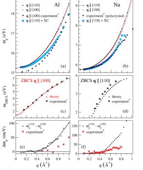
Figure 4: Plasmon dispersion in Al (left column) and Na (right column). (a) and (b) Dispersion of the Drude plasmon for $\mathbf{q}\!\parallel\![110]$ (full black circles) and $\mathbf{q}\!\parallel\![100]$ (open red circles) within the RPA and with the XC correction Utsumi and Ichimaru (1982) (large blue circles). (c) and (d) Dispersion of ZBCS for $\mathbf{q}\!\parallel\![100]$ for Al and for $\mathbf{q}\!\parallel\![110]$ for Na. (e) and (f) Anisotropy of the Drude plasmon. Crosses show the measurements of Refs. Sprösser-Prou et al., 1989^a, vom Felde et al., 1989^b, and Chen and Silcox, 1977^c (extracted from graphical data).

The dispersion $\omega_{\rm p}(q)$ of the Drude plasmon is shown in Fig. 4(a) for $\mathbf{q}\!\parallel\![100]$ and $\mathbf{q}\!\parallel\![110]$. Let us extrapolate the dispersion curves to $q=0$ by fitting the calculated $\omega_{\rm p}(q)$ points with a Lindhard-like function $\omega_{\rm p}(q)=\omega_{\rm p}(0)+\alpha q^{2}+\beta q^{4}$, see Table 1. For Al we obtain $\omega_{\rm p}(0)=15.24$ eV, which is in accord with the value of 15.28 eV calculated in Ref. Lee and Chang (1994) but strongly deviates from the measured value $\omega_{\rm p}(0)=15.01\pm 0.01$ eV Sprösser-Prou et al. (1989). For Na the agreement is much better: $\omega_{\rm p}(0)=5.75$ eV in our theory and 5.76$\pm 0.02$ eV in the experiment vom Felde et al. (1989) (extracted from graphical data).

Table 1: Fitting the plasmon dispersion in Al with the function $\omega_{\rm p}(q)=\omega_{\rm p}(0)+\alpha q^{2}+\beta q^{4}$. XC indicates that a static exchange-correlation correction is included.

	$\omega_{\rm p}(0)$ (eV)	$\alpha$ (eVÅ${}^{2})$	$\beta$ (eVÅ4)
this work $\mathbf{q}\!\parallel\![100]$	15.24	2.75	0.39
this work $\mathbf{q}\!\parallel\![110]$	15.24	2.77	0.49
this work $\mathbf{q}\!\parallel\![100]$ (XC)	15.24	2.03	0.51
this work $\mathbf{q}\!\parallel\![110]$ (XC)	15.24	2.04	0.65
experiment Sprösser-Prou et al. (1989)	15.01	2.27	0.65
theory Lee and Chang (1994) (XC)	15.28	2.13	0.58

Apart from fundamental approximations, the theoretical results suffer from the computational uncertainty of $\epsilon(\omega)$. Indeed, the plasmon energy is determined by the condition $\epsilon_{1}(\omega_{\rm p})=0$, and for a small slope $d\epsilon_{1}(\omega)/d\omega$ it becomes very sensitive to small errors in $\epsilon_{1}(\omega)$. The most important source of error is the inaccuracy of the wave functions $\left\langle\,\mathbf{r}\,|\,\lambda\mathbf{k}\,\right\rangle$, which results in an error in the numerator of Eq. (12). This is an inevitable shortcoming of the variational wave functions, which stems from the incompleteness of the basis set. Its effect on the accuracy of $\omega_{\rm p}$ can be estimated by comparing a numerical $q\to 0$ limit by Eq. (12) with the calculation in the optical limit $q=0$. In the latter case the intraband part $\lambda=\lambda^{\prime}$ acquires the Drude form $\epsilon_{1}(\omega)=1-\omega_{0}^{2}/\omega^{2}$. For a cubic crystal, $\omega_{0}^{2}$ is the diagonal element of the plasma frequency tensor $\omega_{0}=\omega_{xx}=\omega_{yy}=\omega_{zz}$ given by the integral over the Fermi surface

$$\omega_{\mu\nu}^{2}=\frac{1}{\pi^{2}}\sum_{\lambda}\int\frac{v_{\mu}(\lambda\mathbf{k})v_{\nu}(\lambda\mathbf{k})}{|\mathbf{v}(\lambda\mathbf{k})|}\,dS_{\rm F},$$ (13)

where $\mu$ and $\nu$ indicate Cartesian components of the group velocity $\mathbf{v}(\lambda\mathbf{k})$ in the state $\,|\,\lambda\mathbf{k}\,\rangle$. For $\lambda\neq\lambda^{\prime}$ the numerator of Eq. (12) reduces to the squared modulus of the momentum matrix element $\langle\,\lambda^{\prime}\mathbf{k}\,|\,\mathbf{\hat{p}}\,|\,\lambda\mathbf{k}\,\rangle$:

$$\lim_{q\to 0}\langle\,\lambda^{\prime}\mathbf{k}\!+\!\mathbf{q}\,|\,\!\exp(i\mathbf{q}\!\cdot\!\mathbf{r})\!\,|\,\lambda\mathbf{k}\,\rangle=\frac{\hbar}{m}\frac{\langle\,\lambda^{\prime}\mathbf{k}\,|\,\mathbf{\mathbf{q}\!\cdot\!\hat{p}}\,|\,\lambda\mathbf{k}\,\rangle}{E_{\lambda^{\prime}\mathbf{k}}-E_{\lambda\mathbf{k}}}.$$ (14)

In the optical limit we obtain for Al $\omega_{\rm p}^{\rm opt}=15.13$ eV and for Na $\omega_{\rm p}^{\rm opt}=5.72$ eV, i.e., the uncertainty of $\omega_{\rm p}$ amounts to 0.11 eV in Al and 0.03 eV in Na. According to our analysis, most of the error comes from the numerator of the interband term in Eq. (12), and there are two reasons why in Al it is larger than in Na. First, the slope of the $\epsilon_{1}(\omega)$ curve at $\omega_{\rm p}$ is much smaller in Al than in Na: $d\epsilon_{1}(\omega)/d\omega=0.13$ eV^-1 in Al and 0.35 eV^-1 in Na. Second, at $q\to 0$ interband transitions play much larger role in Al than in Na. In Al, the intrinsic uncertainty in $\epsilon_{1}(\omega_{\rm p})$ is 0.014, which is $\sim 4$% of the interband contribution. The error stems form the inaccuracy of the $\psi^{\mathbf{k}}_{\lambda}$ themselves, and it far exceeds the error due to the approximate treatment of the products $\psi^{\mathbf{k}*}_{\lambda^{\prime}}\psi^{\mathbf{k}-\mathbf{q}}_{\lambda}$ with a computationally reasonable product basis set, as we show in Appendix.

IV Anisotropy of plasmon dispersion

The basic aspects of the DF of nearly-free-electron metals can be understood from the Lindhard formula for jellium Lindhard (1954), but the band structure effects have long been realized to be important Bross (1978). In particular, zone boundary collective states were identified in Al Sturm and Oliveira (1984) and in Li and Na Sturm and Oliveira (1989). The relation between the underlying band structure and the energy loss function was analyzed for Al Lee and Chang (1994); Maddocks et al. (1994); Kaltenborn and Schneider (2013) and for alkali metals Taut and Sturm (1992); Quong and Eguiluz (1993); Aryasetiawan and Karlsson (1994); Fleszar et al. (1997); Ku and Eguiluz (1999); Huotari et al. (2009), also under pressure Silkin et al. (2007); Rodriguez-Prieto et al. (2008); Errea et al. (2010); Loa et al. (2011); Attarian Shandiz and Gauvin (2014); Ibañez Azpiroz et al. (2014); Yu et al. (2018). In cesium, the interband transitions were found to cause a negative plasmon dispersion Aryasetiawan and Karlsson (1994); Fleszar et al. (1997). Many works addressed the role of the crystal local field and exchange and correlation (XC) in the dielectric response: the effect of the many-body interactions on the plasmon dispersion was studied for Al and for alkalis in Refs. Quong and Eguiluz, 1993; Cazzaniga et al., 2011; Taut, 1992; Aryasetiawan and Karlsson, 1994; Karlsson and Aryasetiawan, 1995; Fleszar et al., 1997; Ku and Eguiluz, 1999; Huotari et al., 2009; Nechaev et al., 2007; Rodriguez-Prieto et al., 2008; Ibañez Azpiroz et al., 2014. It was concluded that the local fields effects are almost negligible unless the semi-core states are involved Aryasetiawan and Karlsson (1994); Fleszar et al. (1997); Cazzaniga et al. (2011).

Obviously, the anisotropic band structure should lead to the anisotropy of the loss function. The directional dependence of the plasmon dispersion was studied experimentally in Al Urner-Wille and Raether (1976); Petri et al. (1976); Sprösser-Prou et al. (1989), Na vom Felde et al. (1989), and Li Schülke et al. (1986) and theoretically analyzed using model approaches Sturm (1978); Sturm and Oliveira (1989); Bross (1978) and from first principles Taut (1992); Quong and Eguiluz (1993); Lee and Chang (1994); Ku and Eguiluz (1999); Nechaev et al. (2007). In Al and Na the anisotropy of the Drude plasmon is rather subtle: experimentally, the difference $\Delta\omega_{\rm p}=\omega_{\rm p}^{[110]}-\omega_{\rm p}^{[100]}$ reaches $\approx 0.05$ eV around 1 Å^-1 Sprösser-Prou et al. (1989); vom Felde et al. (1989), see Figs. 4(e) and 4(f). The theoretical estimates based on a local pseudopotential model of Bross Bross (1978) and on the ab initio pseudopotential study by Lee and Chang Lee and Chang (1994) gave $\Delta\omega_{\rm p}=0.2$ and 0.25–0.30 eV, respectively. On the contrary, in the ab initio pseudopotential calculation by Quong and Eguiluz Quong and Eguiluz (1993) no anisotropy was resolved.

It is tempting to relate the anisotropy of $\omega_{\rm p}(q)$ to the most conspicuous anisotropic feature of the $\epsilon_{2}(\mathbf{q},\omega)$ spectrum, the zone-boundary gap, see Fig. 3. However, obviously, this feature cannot explain the observation. First, both experimentally and theoretically, Al and Na behave oppositely with respect to the ZBCS: in Al, ZBCS occurs for $\mathbf{q}\!\parallel\![100]$ and in Na for $\mathbf{q}\!\parallel\![110]$, whereas both in Al and in Na it is $\omega_{\rm p}^{[110]}>\omega_{\rm p}^{[100]}$. Second, $\Delta\omega_{\rm p}$ grows with increasing $q$, whereas the influence of the ZB gap decreases, as illustrated by the difference $\epsilon_{2}^{[100]}-\epsilon_{2}^{[110]}$ for Al (and opposite function for Na) shown in Fig. 5. The energy-momentum distributions of the anisotropy are seen to be very similar in Al and Na, with Na[110] playing the role of Al[100] and Na[100] the role of Al[110]. In Al, the $\epsilon_{2}$ spectrum for $\mathbf{q}\!\parallel\![110]$ has a more complicated structure than for $\mathbf{q}\!\parallel\![100]$: apart from the low-energy gap (denoted ZB[110] in Figs. 3 and 5), at larger $q$ there emerges a maximum (denoted $\Omega$[110]) at the high-energy slope of the spectrum. Its contribution to $\epsilon_{1}(\omega_{\rm p})$ grows with $q$, and because it appears below $\omega_{\rm p}^{[110]}$ it shifts $\omega_{\rm p}^{[110]}$ to higher energies. A similar picture takes place for Na, only there is an additional dip-peak structure between ZB[100] and $\Omega$[100], see Fig. 5. However, the effect is the opposite: in Na the $\Omega$[100] peak occurs above the plasmon energy, so that it shifts $\omega_{\rm p}^{[100]}$ to lower energies.

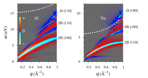
Figure 5: Energy-momentum map of the anisotropy of $\epsilon_{2}$: left graph shows $\omega\epsilon_{2}^{[100]}-\omega\epsilon_{2}^{[110]}$ for Al and right graph shows $\omega\epsilon_{2}^{[110]}-\omega\epsilon_{2}^{[100]}$ for Na. White circles show the location of the Drude plasmon.

Thus, the opposite behavior of the anisotropy of the Drude plasmon relative to ZBCS in Al and Na is explained by the different location of the uppermost structure $\Omega$ relative to $\omega_{\rm p}$. Furthermore, Fig. 5 explains why both in Al and in Na the anisotropy is negligible below and rapidly grows above $q=0.5$ Å^-1, see Figs. 4(e) and 4(f): it is at this wave vector that the $\Omega$-structure appears in the spectrum.

Within the RPA, the difference between the measured and the calculated energies of the Drude plasmon is of the same order of magnitude in Al and Na. The discrepancy is largely due to the neglect of exchange and correlation. These effects can be approximately included by a static local field correction function $G(q)$ using the parametrization of Utsumi and Ichimaru Utsumi and Ichimaru (1982):

$$\epsilon(\mathbf{q},\omega)\to 1+\frac{\epsilon(\mathbf{q},\omega)-1}{1-G(q)\left[\epsilon(\mathbf{q},\omega)-1\right]}.$$ (15)

The XC correction brings the plasmon dispersion in Na into excellent agreement with the experiment over the interval up to $q=0.75$ Å^-1, see Fig. 4(b). For Al, the XC correction transforms the $\omega_{\rm p}(q)$ curve in a similar way, see Fig. 4(a), but the parameter $\alpha$ is strongly underestimated, see Table.

In contrast to Al and Na, in alkali metals Li, K, Rb, and Cs the interband transitions around the plasmon energy are rather intense, see Fig. 6. Their strong energy dependence causes more or less pronounced irregularities in the plasmon dispersion accompanied by a strong damping (large spectral width) of the plasmon. Also the anisotropy of $\epsilon_{2}(\omega)$ is very strong, which leads to a rather different shape of the plasmon dispersion curve for different directions of $\mathbf{q}$, see Fig. 6.

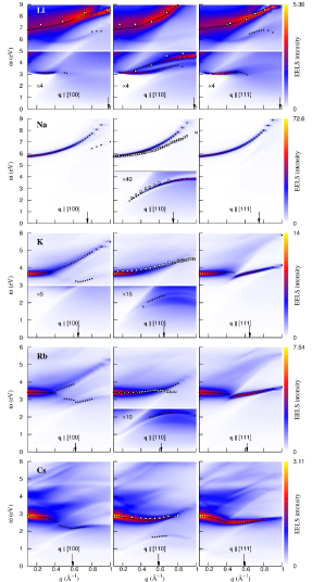
Figure 6: Calculated energy loss spectra of Li, Na, K, Rb, and Cs for $\mathbf{q}\!\parallel\![100]$, $\mathbf{q}\!\parallel\![110]$, and $\mathbf{q}\!\parallel\![111]$. White squares are experimental data of Refs. Schülke et al., 1986, 1984 for Li and of Ref. vom Felde et al., 1989 for Na, K, Rb, and Cs. Black circles show the plasmon location, i.e., $\epsilon_{1}(q,\omega)=0$. The vertical arrows indicate the critical $q$ values of the Lindhard model. Note the scale change indicated by the horizontal white line.

Figure 6 show the loss function of alkali metals for $\mathbf{q}\!\parallel\![100]$, $\mathbf{q}\!\parallel\![110]$, and $\mathbf{q}\!\parallel\![111]$ in comparison with the experiment. In Li, we again observe both the Drude plasmon at $\omega_{\rm p}(0)=6.72$ eV and the ZBCS. For $\mathbf{q}\!\parallel\![110]$, in our calculation two ZBCS branches are resolved. In K, the plasmon peaks are much sharper than in Li, but the band-structure effects are, evidently, very strong: the plasmon dispersion is far from parabolic, and its shape is considerably different for different directions. For $\mathbf{q}\!\parallel\![110]$, the agreement with the experiment vom Felde et al. (1989) is rather good. (In contrast to Al and Na, in K the experimental curve lies slightly above the theoretical one.) In Rb and Cs, the unoccupied $3d$ states come closer to the Fermi level, and the strong dipole transitions to these states are responsible for the pronouncedly non-free-electron behavior of the DF Aryasetiawan and Karlsson (1994): in Rb the plasmon disperses only weakly, and in Cs the function $\omega_{\rm p}(q)$ is non-monotonic, with a minimum at $\sim$0.5 Å^-1 in agreement with the experiment vom Felde et al. (1989). Our result is in good agreement with the pseudopotential calculation of Ref. Fleszar et al., 1997.

V Summary

We have developed a product basis set to represent response functions within an all-electron framework. The proposed basis set consists of plane waves defined over the whole space and spatially restricted orbitals, with the spatial dependence of the response function being smoothly continuous by construction. It has a number of physically appealing and computationally convenient properties. In particular, it can be defined universally, without regard to the computational parameters of the band structure method (such as muffin-tin radii, energy parameters, and number of APWs in LAPW). Consequently, the accuracy with which the physically relevant response is represented can be set a priori and balanced with the intrinsic accuracy of the underlying band structure calculation. Depending on the specific application, the basis set can be optimized by tuning the relative weight carried by PWs and IOs.

We have implemented the scheme into the extended LAPW method and studied both the accuracy of the representation of the dielectric function and the intrinsic accuracy of the underlying wave functions.

We have applied the new method to the dielectric function of cubic $sp$ metals Al, Li, Na, K, Rb, and Cs with the aim to understand what can be learned from the anisotropy of their bulk loss function. In the non-free-electron-like metals Li, K, Rb, and Cs the anisotropy of the plasmon dispersion is rather irregular due to the vicinity of the intra- and interband transitions to the plasmon. In contrast, in Al and Na, the plasmon occurs well above the intense interband transitions, and their effect is much tinier. We have reproduced the sign and the qualitative trend of the $\mathbf{q}$ dependence of the anisotropy in both metals, although the absolute values are substantially overestimated in the calculation. We revealed a strong similarity of the structure of the particle-hole transitions in Al and Na and traced the plasmon anisotropy to the energy location of the plasmon relative to very subtle features of the imaginary DF, which are barely visible in the $\epsilon_{2}(\omega)$ spectrum. Our analysis demonstrates that the EELS experiment is sensitive to subtle details of the unoccupied bulk band structure and may give access to features not reachable with angle-integrated (optics) or surface-sensitive electron spectroscopies.

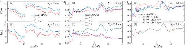
Figure 7: Convergence of MME with the angular-momentum cutoff $l_{\text{max}}$, (a)–(d), and with the number of plane-waves, (e) and (f). For Cs, (a) and (b), $\mathbf{k}$-averaged MME $R(\omega)$ are shown in logarithmic scale (a) for $S_{\gamma}=3$ a.u. and (b) for $S_{\gamma}=5$ a.u. The Fourier part comprises 229 PWs. Vertical arrows in the upper $\omega$-axes mark the onset of the semi-core transitions. For Cu, $S_{\gamma}=1.2$ a.u. in (c) and (e) and $S_{\gamma}=2.4$ a.u. in (d) and (f). In (c) and (d), the Fourier part comprises 459 PWs. In (e) and (f), the convergence with the number of PWs is for $l_{\text{max}}=4$. The cutoff energy $|\mathbf{G}|^{2}$ is given in parentheses.

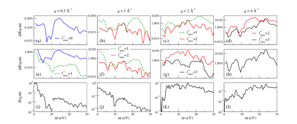
Figure 8: Convergence of the Rayleigh expansion of $\exp(i\mathbf{q}\!\cdot\!\mathbf{r})$ for Cs for $\mathbf{q}\!\parallel\![100]$ for $q=0.5$, 1.0, 2.0, and 4.0 Å^-1for $S_{\gamma}=3$ a.u. (a)–(d) and for $S_{\gamma}=5$ a.u. (e)–(h). The lowest row shows the reference spectrum $\bar{R}(q,\omega)$ calculated with $l^{\prime\prime}_{\rm max}=4$, see Eq. (9). The upper rows show $\mathbf{k}$-averaged values of the error $\Delta R(l^{\prime\prime}_{\rm max})=|R(l^{\prime\prime}_{\rm max})-\bar{R}|$ with $l_{\rm max}=0$ to 3 [in percent relative to the average value of $\bar{R}(q,\omega)$ over the spectrum, note the logarithmic scale]. The Fourier part comprises 959 PWs.

*

Appendix A Accuracy and convergence

Let us study the properties of the product basis set regarding the plane-wave cutoff of $\psi^{\text{F}}$ and the angular-momentum cutoff of $\psi^{\text{I}}$, see Eq. (6). We first consider the momentum operator $\hat{\mathbf{p}}=-i\hbar\boldsymbol{\nabla}$, which is related to the $q\to 0$ limit of the operator $\exp(i\mathbf{q}\cdot\mathbf{r})/q$, see Eq. (14). This will give the idea of the accuracy of the filtered wave functions because the operator $\hat{\mathbf{p}}$ itself is treated exactly, and the result can be compared with the exact value calculated from the complete APW representation of the wave function. To have an idea of the accuracy of the momentum matrix elements (MME), let us consider its $\mathbf{k}$-averaged value, which we define as the ratio of the absorption probability

$$W(\omega)=\sum_{mn}\,\int_{\rm BZ}\!\!\!d\mathbf{k}\,P^{\mathbf{k}}_{mn}\,\delta(E_{n}^{\mathbf{k}}-E_{m}^{\mathbf{k}}-\hbar\omega)$$ (16)

to the joint density of states $J(\omega)$, which is obtained by setting the transition probability $P^{\mathbf{k}}_{mn}$ in Eq. (16) to unity,

$$R(\omega)=W(\omega)/J(\omega).$$ (17)

The sum in Eq. (16) runs over all occupied states $\,|\,n\mathbf{k}\,\rangle$ and unoccupied states $\,|\,m\mathbf{k}\,\rangle$. For a cubic crystal the dipole transition probability is $P^{\mathbf{k}}_{mn}=\frac{1}{3}\left|\langle\,m\mathbf{k}\,|\,\hat{\mathbf{p}}\,|\,n\mathbf{k}\,\rangle\right|^{2}$.

It follows from the dipole selection rules that for reasonably small values of $S_{\gamma}$ the $l_{\text{max}}$-cutoff in Eq. (9) does not need to exceed the highest angular momentum of the atomic valence shell plus one. This is illustrated for Cs in Figs. 7(a) and 7(b) and for Cu in Figs. 7(c) and 7(d). Surprisingly, for Cs, not only for a moderate $S_{\gamma}=3$ a.u. but also for a very large $S_{\gamma}=5$ a.u. at $l_{\text{max}}=2$ the error is negligible. Note that the results with the smaller $S_{\gamma}$ are slightly more accurate although a larger part of the wave function is described by plane waves. While for Cs the challenging aspect is the angular-momentum expansion of $\psi^{\text{I}}$ in a large sphere, for Cu it is the plane-wave expansion of $\psi^{\text{F}}$. Figures 7(e) and  7(f) show the PW-convergence of the momentum matrix elements (MME) for $S_{\gamma}=1.2$ and 2.4 a.u., respectively. Note that for $S_{\gamma}=2.4$ a.u., which is close to the MT radius, $R(\omega)$ converges already at 89 PWs, which equals the number of APWs needed to obtain the band structure. The obvious advantage of the new basis is that PWs are orthogonal and the momentum operator is diagonal.

For the operator $\exp(i\mathbf{q}\!\cdot\!\mathbf{r})$ there arises the question of the convergence of its Rayleigh expansion, i.e., of the sum over $l^{\prime\prime}$ in Eq. (9). The convergence of the $\mathbf{k}$-averaged matrix element $\left|\langle\,m\mathbf{k}+\mathbf{q}\,|\,\exp(i\mathbf{q}\!\cdot\!\mathbf{r})\,|\,n\mathbf{k}\,\rangle\right|^{2}$ is illustrated in Fig. 8 for Cs for $S_{\gamma}=3$ and 5 a.u. The role of quadrupole transitions is seen to increase with $q$, especially for the larger $S_{\gamma}$. Interestingly, the quadrupole transitions from the semicore $5p$ states are more intense than from the valence band. Figure 8 demonstrates that the $l^{\prime\prime}$ convergence can be accelerated by diminishing the $\gamma$-sphere.

References

- Giuliani and Vignale (2005) G. Giuliani and G. Vignale, Quantum Theory of the Electron Liquid, Masters Series in Physics and Astronomy (Cambridge University Press, 2005).
- Hedin (1965) L. Hedin, New method for calculating the one-particle green’s function with application to the electron-gas problem, Phys. Rev. 139, A796 (1965).
- Aryasetiawan and Gunnarsson (1998) F. Aryasetiawan and O. Gunnarsson, The GW method, Reports on Progress in Physics 61, 237 (1998).
- Haug and Koch (2004) H. Haug and S. Koch, Quantum Theory of the Optical and Electronic Properties of Semiconductors (World Scientific, 2004).
- Pines (1963) D. Pines, Elementary Excitations in Solids, Lecture notes and supplements in physics (Benjamin, 1963).
- Feibelman (1982) P. J. Feibelman, Surface electromagnetic fields, Progress in Surface Science 12, 287 (1982).
- Liebsch (1997) A. Liebsch, Electronic excitations at metal surfaces (Plenum, New-York, 1997).
- Pitarke et al. (2007) J. M. Pitarke, V. M. Silkin, E. V. Chulkov, and P. M. Echenique, Theory of surface plasmons and surface-plasmon polaritons, Reports on Progress in Physics 70, 1 (2007).
- Krasovskii et al. (2010) E. E. Krasovskii, V. M. Silkin, V. U. Nazarov, P. M. Echenique, and E. V. Chulkov, Dielectric screening and band-structure effects in low-energy photoemission, Phys. Rev. B 82, 125102 (2010).
- Siek et al. (2017) F. Siek, S. Neb, P. Bartz, M. Hensen, C. Strüber, S. Fiechter, M. Torrent-Sucarrat, V. Silkin, E. Krasovskii, N. Kabachnik, S. Fritzsche, R. Muiño, P. Echenique, A. Kazansky, N. Müller, W. Pfeiffer, and U. Heinzmann, Angular momentum–induced delays in solid-state photoemission enhanced by intra-atomic interactions, Science 357, 1274 (2017).
- Nazarov et al. (2017) V. U. Nazarov, V. M. Silkin, and E. E. Krasovskii, Probing mesoscopic crystals with electrons: One-step simultaneous inelastic and elastic scattering theory, Phys. Rev. B 96, 235414 (2017).
- Harriman (1986) J. E. Harriman, Densities, operators, and basis sets, Phys. Rev. A 34, 29 (1986).
- Payne et al. (1992) M. C. Payne, M. P. Teter, D. C. Allan, T. A. Arias, and J. D. Joannopoulos, Iterative minimization techniques for ab initio total-energy calculations: molecular dynamics and conjugate gradients, Rev. Mod. Phys. 64, 1045 (1992).
- Blöchl (1994) P. E. Blöchl, Projector augmented-wave method, Phys. Rev. B 50, 17953 (1994).
- Brodersen et al. (2002) S. Brodersen, D. Lukas, and W. Schattke, Calculation of the dielectric function in a local representation, Phys. Rev. B 66, 085111 (2002).
- Mortensen et al. (2005) J. J. Mortensen, L. B. Hansen, and K. W. Jacobsen, Real-space grid implementation of the projector augmented wave method, Phys. Rev. B 71, 035109 (2005).
- Yan et al. (2011) J. Yan, J. J. Mortensen, K. W. Jacobsen, and K. S. Thygesen, Linear density response function in the projector augmented wave method: Applications to solids, surfaces, and interfaces, Phys. Rev. B 83, 245122 (2011).
- Blase and Ordejón (2004) X. Blase and P. Ordejón, Dynamical screening and absorption within a strictly localized basis implementation of time-dependent LDA: From small clusters and molecules to aza-fullerenes, Phys. Rev. B 69, 085111 (2004).
- Umari et al. (2009) P. Umari, G. Stenuit, and S. Baroni, Optimal representation of the polarization propagator for large-scale calculations, Phys. Rev. B 79, 201104 (2009).
- Aryasetiawan and Gunnarsson (1994) F. Aryasetiawan and O. Gunnarsson, Product-basis method for calculating dielectric matrices, Phys. Rev. B 49, 16214 (1994).
- Foerster (2008) D. Foerster, Elimination, in electronic structure calculations, of redundant orbital products, J. Chem. Phys. 128, 034108 (2008).
- Slater (1937) J. C. Slater, Wave functions in a periodic potential, Phys. Rev. 51, 846 (1937).
- Andersen (1975) O. K. Andersen, Linear methods in band theory, Phys. Rev. B 12, 3060 (1975).
- Koelling and Arbman (1975) D. D. Koelling and G. O. Arbman, Use of energy derivative of the radial solution in an augmented plane wave method: application to copper, J. Phys. F: Met. Phys. 5, 2041 (1975).
- Singh (1991) D. Singh, Ground-state properties of lanthanum: Treatment of extended-core states, Phys. Rev. B 43, 6388 (1991).
- Krasovskii (1997) E. E. Krasovskii, Accuracy and convergence properties of the extended linear augmented-plane-wave method, Phys. Rev. B 56, 12866 (1997).
- Jiang et al. (2013) H. Jiang, R. I. Gómez-Abal, X.-Z. Li, C. Meisenbichler, C. Ambrosch-Draxl, and M. Scheffler, FHI-gap: A GW code based on the all-electron augmented plane wave method, Computer Physics Communications, 184, 348–366 (2013).
- Friedrich et al. (2010) C. Friedrich, S. Blügel, and A. Schindlmayr, Efficient implementation of the approximation within the all-electron FLAPW method, Phys. Rev. B 81, 125102 (2010).
- Nabok et al. (2016) D. Nabok, A. Gulans, and C. Draxl, Accurate all-electron quasiparticle energies employing the full-potential augmented plane-wave method, Phys. Rev. B 94, 035118 (2016).
- Kotani and van Schilfgaarde (2002) T. Kotani and M. van Schilfgaarde, All-electron GW approximation with the mixed basis expansion based on the full-potential LMTO method, Solid State Commun. 121, 461 (2002).
- Friedrich et al. (2011) C. Friedrich, M. C. Müller, and S. Blügel, Band convergence and linearization error correction of all-electron calculations: The extreme case of zinc oxide, Phys. Rev. B 83, 081101 (2011).
- Foo and Hopfield (1968) E.-N. Foo and J. J. Hopfield, Optical absorption and energy loss in sodium in the Hartree approximation, Phys. Rev. 173, 635 (1968).
- Krasovskii and Schattke (2001) E. E. Krasovskii and W. Schattke, Semirelativistic technique for calculations: Optical properties of Pd and Pt, Phys. Rev. B 63, 235112 (2001).
- Michalicek et al. (2013) G. Michalicek, M. Betzinger, C. Friedrich, and S. Blügel, Elimination of the linearization error and improved basis-set convergence within the FLAPW method, Computer Physics Communications 184, 2670 (2013).
- Krasovskii et al. (1999) E. E. Krasovskii, F. Starrost, and W. Schattke, Augmented fourier components method for constructing the crystal potential in self-consistent band-structure calculations, Phys. Rev. B 59, 10504 (1999).
- Krasovskii and Schattke (1999) E. E. Krasovskii and W. Schattke, Local field effects in optical excitations of semicore electrons, Phys. Rev. B 60, R16251 (1999).
- Betzinger et al. (2011) M. Betzinger, C. Friedrich, S. Blügel, and A. Görling, Local exact exchange potentials within the all-electron FLAPW method and a comparison with pseudopotential results, Phys. Rev. B 83, 045105 (2011).
- Koval et al. (2014) P. Koval, D. Foerster, and D. Sánchez-Portal, Fully self-consistent and quasiparticle self-consistent for molecules, Phys. Rev. B 89, 155417 (2014).
- Jiang (2018) H. Jiang, Revisiting the approach to - and -electron oxides, Phys. Rev. B 97, 245132 (2018).
- Aryasetiawan and Karlsson (1994) F. Aryasetiawan and K. Karlsson, Energy loss spectra and plasmon dispersions in alkali metals: Negative plasmon dispersion in Cs, Phys. Rev. Lett. 73, 1679 (1994).
- Fleszar et al. (1997) A. Fleszar, R. Stumpf, and A. G. Eguiluz, One-electron excitations, correlation effects, and the plasmon in cesium metal, Phys. Rev. B 55, 2068 (1997).
- Cazzaniga et al. (2011) M. Cazzaniga, H.-C. Weissker, S. Huotari, T. Pylkkänen, P. Salvestrini, G. Monaco, G. Onida, and L. Reining, Dynamical response function in sodium and aluminum from time-dependent density-functional theory, Phys. Rev. B 84, 075109 (2011).
- Ehrenreich and Cohen (1959) H. Ehrenreich and M. H. Cohen, Self-consistent field approach to the many-electron problem, Phys. Rev. 115, 786 (1959).
- Lehmann and Taut (1972) G. Lehmann and M. Taut, On the numerical calculation of the density of states and related properties, Physica Status Solidi (b) 54, 469 (1972).
- Lee and Chang (1994) K.-H. Lee and K. J. Chang, First-principles study of the optical properties and the dielectric response of Al, Phys. Rev. B 49, 2362 (1994).
- Lindhard (1954) J. Lindhard, On the properties of a gas of charged particles, K. Dan. Vidensk. Selsk. Mat.-Fys. Medd. 28, 1 (1954).
- Utsumi and Ichimaru (1982) K. Utsumi and S. Ichimaru, Dielectric formulation of strongly coupled electron liquids at metallic densities. VI. analytic expression for the local-field correction, Phys. Rev. A 26, 603 (1982).
- Sprösser-Prou et al. (1989) J. Sprösser-Prou, A. vom Felde, and J. Fink, Aluminum bulk-plasmon dispersion and its anisotropy, Phys. Rev. B 40, 5799 (1989).
- vom Felde et al. (1989) A. vom Felde, J. Sprösser-Prou, and J. Fink, Valence-electron excitations in the alkali metals, Phys. Rev. B 40, 10181 (1989).
- Chen and Silcox (1977) C. H. Chen and J. Silcox, Direct nonvertical interband transitions at large wave vectors in aluminum, Phys. Rev. B 16, 4246 (1977).
- Bross (1978) H. Bross, Pseudopotential theory of the dielectric function of Al-the volume plasmon dispersion, J. Phys. F: Met. Phys. 8, 2631 (1978).
- Sturm and Oliveira (1984) K. Sturm and L. E. Oliveira, Theory of a zone-boundary collective state in Al: A model calculation, Phys. Rev. B 30, 4351 (1984).
- Sturm and Oliveira (1989) K. Sturm and L. E. Oliveira, Zone boundary collective states in lithium and sodium, EPL (Europhysics Letters) 9, 257 (1989).
- Maddocks et al. (1994) N. E. Maddocks, R. W. Godby, and R. J. Needs, Bandstructure effects in the dynamic response of aluminium, EPL (Europhysics Letters) 27, 681 (1994).
- Kaltenborn and Schneider (2013) S. Kaltenborn and H. C. Schneider, Plasmon dispersions in simple metals and Heusler compounds, Phys. Rev. B 88, 045124 (2013).
- Taut and Sturm (1992) M. Taut and K. Sturm, Plasmon dispersion constant of the alkali metals, Solid State Commun. 82, 295 (1992).
- Quong and Eguiluz (1993) A. A. Quong and A. G. Eguiluz, First-principles evaluation of dynamical response and plasmon dispersion in metals, Phys. Rev. Lett. 70, 3955 (1993).
- Ku and Eguiluz (1999) W. Ku and A. G. Eguiluz, Plasmon lifetime in K: A case study of correlated electrons in solids amenable to ab initio theory, Phys. Rev. Lett. 82, 2350 (1999).
- Huotari et al. (2009) S. Huotari, C. Sternemann, M. C. Troparevsky, A. G. Eguiluz, M. Volmer, H. Sternemann, H. Müller, G. Monaco, and W. Schülke, Strong deviations from jellium behavior in the valence electron dynamics of potassium, Phys. Rev. B 80, 155107 (2009).
- Silkin et al. (2007) V. M. Silkin, A. Rodriguez-Prieto, A. Bergara, E. V. Chulkov, and P. M. Echenique, Strong variation of dielectric response and optical properties of lithium under pressure, Phys. Rev. B 75, 172102 (2007).
- Rodriguez-Prieto et al. (2008) A. Rodriguez-Prieto, V. M. Silkin, A. Bergara, and P. M. Echenique, Energy loss spectra of lithium under pressure, New J. Phys. 10, 053035 (2008).
- Errea et al. (2010) I. Errea, A. Rodriguez-Prieto, B. Rousseau, V. M. Silkin, and A. Bergara, Electronic collective excitations in compressed lithium from ab initio calculations: Importance and anisotropy of local-field effects at large momenta, Phys. Rev. B 81, 205105 (2010).
- Loa et al. (2011) I. Loa, K. Syassen, G. Monaco, G. Vankó, M. Krisch, and M. Hanfland, Plasmons in sodium under pressure: Increasing departure from nearly free-electron behavior, Phys. Rev. Lett. 107, 086402 (2011).
- Attarian Shandiz and Gauvin (2014) M. Attarian Shandiz and R. Gauvin, Density functional and theoretical study of the temperature and pressure dependency of the plasmon energy of solids, Journal of Applied Physics 116, 163501 (2014).
- Ibañez Azpiroz et al. (2014) J. Ibañez Azpiroz, B. Rousseau, A. Eiguren, and A. Bergara, Ab initio analysis of plasmon dispersion in sodium under pressure, Phys. Rev. B 89, 085102 (2014).
- Yu et al. (2018) Z. Yu, H. Y. Geng, Y. Sun, and Y. Chen, Optical properties of dense lithium in electride phases by first-principles calculations, Sci. Rep. 8, 3868 (2018).
- Taut (1992) M. Taut, Exchange-correlation correction to the dielectric function of the inhomogeneous electron gas, J. Phys.: Condens. Matter 4, 9595 (1992).
- Karlsson and Aryasetiawan (1995) K. Karlsson and F. Aryasetiawan, Plasmon lifetime, zone-boundary collective states, and energy-loss spectra of lithium, Phys. Rev. B 52, 4823 (1995).
- Nechaev et al. (2007) I. A. Nechaev, V. M. Silkin, and E. V. Chulkov, Inclusion of the exchange-correlation effects in ab initio methods for calculating the plasmon dispersion and line width in metals, Physics of the Solid State 49, 1820 (2007).
- Urner-Wille and Raether (1976) M. Urner-Wille and H. Raether, Anisotropy of the 15 eV volume plasmon dispersion in a1, Phys. Lett. A 58, 265 (1976).
- Petri et al. (1976) E. Petri, A. Otto, and W. Hanke, Anisotropy of plasmon dispersion in Al: An electron correlation effect, Solid State Commun. 19, 711 (1976).
- Schülke et al. (1986) W. Schülke, H. Nagasawa, S. Mourikis, and P. Lanzki, Dynamic structure of electrons in Li metal: Inelastic synchrotron x-ray scattering results and interpretation beyond the random-phase approximation, Phys. Rev. B 33, 6744 (1986).
- Sturm (1978) K. Sturm, Band structure effects on the plasmon dispersion in simple metals, Zeitschrift für Physik B Condensed Matter 29, 27 (1978).
- Schülke et al. (1984) W. Schülke, H. Nagasawa, and S. Mourikis, Dynamic structure factor of electrons in Li by inelastic synchrotron x-ray scattering, Phys. Rev. Lett. 52, 2065 (1984).