Octagons I: Combinatorics
and Non-Planar Resummations

1 Introduction

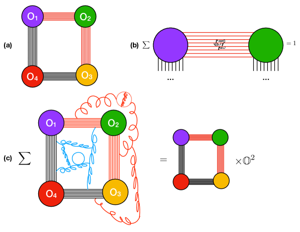
Figure 1: Large cyclic operators at genus zero. (a) The tree-level result is given by a single Feynman graph of rectangular form. For large operators, this rectangle creates a big frame. (b) The frame, when big, does not receive loop corrections because of supersymmetry. Indeed these loop corrections are indistinguishable from those arising in the two-point function of BPS operators, a protected quantity. (c) The inside and the outside of the frame, on the other hand, are loop corrected. The sum of all quantum corrections to the inside (or outside) define a function $\mathbb{O}$ of the ’t Hooft coupling and of the four-point cross ratio.

In this work, we will consider correlation functions of single-trace half-BPS operators in $\mathcal{N}=4$ super Yang–Mills theory. Each of these operators creates a closed string state, so these correlation functions describe closed-string scattering in $\mathrm{AdS}_{5}\times\mathrm{S}^{5}$.

We will focus on four-point correlation functions in an interesting limit of very large BPS operators with carefully chosen polarizations, where the closed string scattering process factorizes into several copies of an off-shell open string partition function $\mathbb{O}$ that was determined exactly in [1, 2] at any value of the ’t Hooft coupling and further simplified into an infinite determinant representation in [3].

The dimensions of the operators we will consider scale with the rank of the $U(N_{\text{c}})$ gauge group as $\sqrt{N_{\text{c}}}$, reminiscent of inspiring earlier studies [4, 5, 6, 7, 8] in the plane-wave Berenstein–Maldacena–Nastase (BMN) limit [9]. The motivation for this particular limit is similar to the one considered in those works: It will allow us to re-sum the large $N_{\text{c}}$ ’t Hooft expansion. We now have a much stronger control over the ’t Hooft coupling behavior due to integrability and bootstrap techniques that were not yet available at the time, so it seems rather timely to revive those explorations in light of these newer technologies.

A key difference compared to the earlier BMN-related works [4, 5, 6, 7, 8] is that in those studies there was typically a single R-charge that was taken to be large, while for the present work it is crucial that the operators correspond to closed strings rotating in different $\mathrm{S}^{5}$ equators. To be precise, we will take two operators to be two different BMN highest-weight states

$$\mathcal{O}_{2}=\operatorname{tr}({\color[rgb]{1,0,0}X}^{2k}\,)(z)\,,\quad\mathcal{O}_{4}=\operatorname{tr}(Z^{2k})(\infty)\,,$$ (1.1)

and two other operators to be two equal BMN descendants

$$\mathcal{O}_{1}=\operatorname{tr}(\bar{Z}^{k}\,{\color[rgb]{1,0,0}\bar{X}}^{k})(0)+\texttt{permutations}\,,\quad\mathcal{O}_{3}=\operatorname{tr}(\bar{Z}^{k}\,{\color[rgb]{1,0,0}\bar{X}}^{k})(1)+\texttt{permutations}\,,$$ (1.2)

where $X$ and $Z$ are two complex scalars in $\mathcal{N}=4$. This choice of two highest-weight states and two BMN descendents might seem asymmetric and unorthodox but is actually quite important, both technically and physically.

The technical simplification can already be seen at tree level in the planar limit: Because of R-charge conservation, there is only a single Feynman diagram computing the four-point correlation function! The correlator is simply given by a product of $4k$ propagators, with $k$ parallel propagators connecting each pair of consecutive operators $\mathcal{O}_{i}$ and $\mathcal{O}_{i+1}$, thus drawing a square frame as depicted in Figure 1(a).

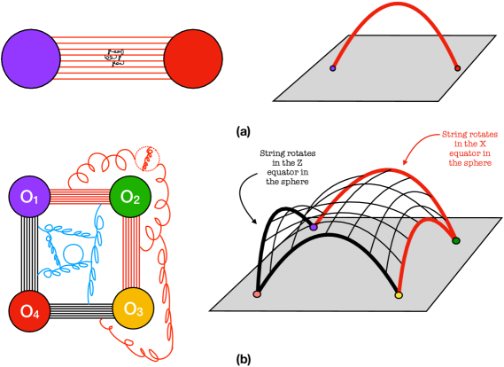
Figure 2: Each bundle of propagators in the field theory can be thought of as a very heavy BMN string geodesic which is protected by supersymmetry. The octagon is the sum of all Feynman diagrams inside (or outside) the tree level frame or, equivalently, the top (or bottom) of the folded string stretching between four consecutive geodesics. At genus zero, the folded string has a top and bottom and hence the result is given by $\mathbb{O}^{2}$ in agreement with the field theory result.

Beyond tree level – but still at genus zero – we decorate this correlator by all possible Feynman loops. The diagrams inside individual propagator bundles connecting two operators – as depicted in Figure 1(b) – cancel out by supersymmetry, so they do not correct the correlator. After all, those diagrams do not know they belong to a four-point function rather than a protected two-point function of BPS operators. The diagrams inside the square – represented in Figure 1(c) – do probe all four operators and hence lead to a non-trivial function $\mathbb{O}$ that depends on the ’t Hooft coupling $\mafx@lambda$ and on the conformal cross ratios formed by the four operators. This function $\mathbb{O}$ was studied in detail in [1, 2]. The diagrams outside the square contribute by the same amount as the diagrams inside, hence the full genus-zero result is simply given by (throughout this work, $g$ denotes the genus)

$$\langle\mathcal{O}_{1}\dots\mathcal{O}_{4}\rangle_{g=0}=\langle\mathcal{O}_{1}\dots\mathcal{O}_{4}\rangle_{\mafx@lambda=0,g=0}\times\mathbb{O}^{2}\,.$$ (1.3)

Note that if it were not for large $k$, the decoupling between outside and inside would be absent. Indeed, for any finite $k$ and large enough loop order, diagrams can communicate all the way from the inside to the outside.

(a) $\mathbb{O}^{0}$	(b) $\mathbb{O}^{2}$	(c) $\mathbb{O}^{4}$

Figure 3: Four operators (circles) are inserted on a torus (the top and bottom sides as well as the left and right sides of the square are identified). Wick contractions organize into skeleton graphs, where each edge (black line) is a bundle of parallel propagators. For our choice of operators, all faces of all skeleton graphs are octagons. Shown in shades of gray are octagons that touch only two or three of the operators, these are protected by supersymmetry. Octagons that touch all four operators (blue shades) are non-trivial functions of the ’t Hooft coupling and conformal cross ratios.

In dual string theory terms, each bundle of propagators connecting consecutive BPS operators can be thought of as a heavy geodesic connecting points $x_{i}$ and $x_{i+1}$ on the AdS boundary, as represented in Figure 2(a). Because there are so many propagators $k$ in each bundle, these geodesics are very heavy and will not move away from their classical configuration. The four classical geodesics will be connected by a folded string, as depicted in Figure 2(b). The fold lines are given by the heavy geodesics, which effectively decouple the top and bottom of the folded string. The two sides of the folded string are the string counterpart to the gauge-theory Feynman diagrams inside and outside of the square. In contrast to the heavy geodesics, they do vibrate quantum mechanically, each of them thus defining a full-fledged open string partition function – this open string partition function is the string definition of the function $\mathbb{O}$.

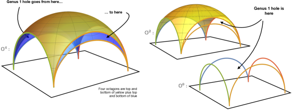
Figure 4: AdS embeddings of the three graphs in Figure 3. Each edge in Figure 3 represents a bundle of $\mathcal{O}(\sqrt{N_{\text{c}}})$ propagators, and therefore becomes a heavy BMN geodesic connecting two operators. These geodesics are folds of the worldsheet that connect adjacent octagons. The BPS octagons have no extent in AdS, they curl up along the BMN geodesics. The non-BPS octagons are extended objects that touch all four operators.

This concludes the genus-zero considerations. This paper’s main focus is on the higher-genus picture. We will explain the general structure of the correlator in detail in the next section. The upshot is that (i) the leading term in the large-$k$ limit at fixed genus $g$ is proportional to $k^{4g}$, and (ii) we can can stack from zero to $2g+2$ folded strings on top of each other to construct a genus-$g$ surface. Since each fold joins two open strings, the number of open string surfaces ought to be even, and thus the full correlation function, i. e. the full closed-string partition function – in the limit of large $k$ – will be simply given by a polynomial $P_{g+1}$ of degree $g+1$ in the square of the open string partition function $\mathbb{O}$,

$$\langle\mathcal{O}_{1}\dots\mathcal{O}_{4}\rangle=\langle\mathcal{O}_{1}\dots\mathcal{O}_{4}\rangle_{\mafx@lambda=0,g=0}\times\left[\mathbb{O}^{2}+\frac{k^{4}}{N_{\text{c}}^{2}}P_{2}(\mathbb{O}^{2})+\frac{k^{8}}{N_{\text{c}}^{4}}P_{3}(\mathbb{O}^{2})+\dots\right]\,.$$ (1.4)

Resumming the full large $N_{\text{c}}$ expansion, at any value of the ’t Hooft coupling, thus amounts to finding the function of two variables

$$\mathcal{A}(\mafx@zeta,\mathbb{O})\equiv\lim_{N_{\text{c}}\to\infty}\left.\frac{\langle\mathcal{O}_{1}\dots\mathcal{O}_{4}\rangle}{\langle\mathcal{O}_{1}\dots\mathcal{O}_{4}\rangle_{\mafx@lambda=0,g=0}}\right|_{k=\mafx@zeta\sqrt{N_{\text{c}}}}\,.$$ (1.5)

Note that this correlation function $\mathcal{A}$ depends very non-trivially on the conformal cross ratios and on the ’t Hooft coupling of the theory through the octagon function $\mathbb{O}$ computed in [1, 2]. The main result of this paper is a representation of the function $\mathcal{A}$ and of the associated polynomials $P_{g+1}$ in (1.4) in terms of a matrix model, where the octagon function $\mathbb{O}$ enters as an effective quartic coupling.

2 A Matrix Model for Large Operators

The basis of our computation is the (planar and non-planar) hexagonalization prescription for correlation functions [10, 11, 12, 13, 14, 15]. The starting point of that prescription is a sum over all Wick contractions of the free gauge theory. We organize this sum by first summing over “skeleton graphs” of the desired genus. Each edge in a skeleton graph represents a bundle of one or more parallel propagators. For each skeleton graph, we then sum over all possible ways of distributing propagators on the edges of the graph (that are compatible with the charges of the operators).

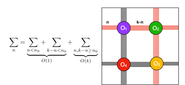
Figure 5: Octopus principle. Configurations where some available propagator bundles are not massively occupied are strongly suppressed in the large charge limit. All skeleton graphs are thus maximal graphs, where no further propagator bundle can be added without increasing the genus at hand.

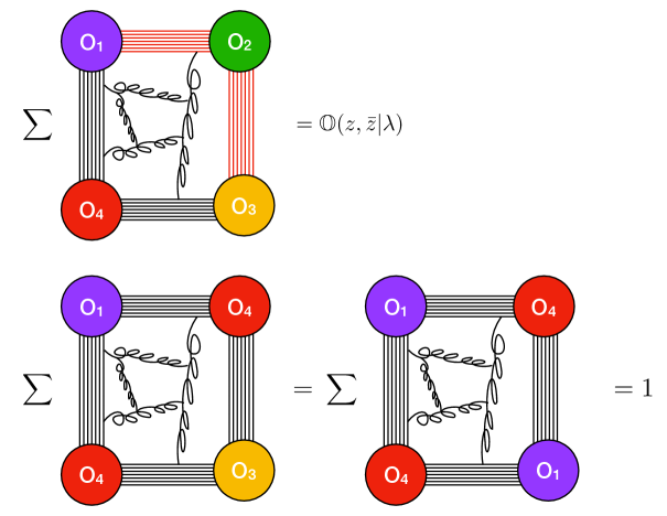
Figure 6: The three types of squares all large-$k$ skeleton graphs are made of, see (2.2). Squares can connect all four operators (top figure), and all such squares equal the non-trivial function $\mathbb{O}$ of the ’t Hooft coupling $\mafx@lambda$ and the cross ratios parametrized by $z$ and $\bar{z}$. Squares may also only connect three operators (bottom left) or two operators (bottom right), such squares are protected by supersymmetry and hence do not receive loop corrections.

We saw in the introduction that, for our choice of operators, there is only a single skeleton graph at genus zero. At higher genus, there are several contributing diagrams. For example, the top row of Figure 3 shows three different genus-one graphs contributing to the four-point correlation function of our operators (1.1), (1.2). The key observation illustrated by these examples is the following: For large operators, at any genus order, all skeleton graphs that contribute are quadrangulations, i. e. all faces of these graphs are quadrangles. This is because of what we call the octopus principle. It comes about because we have to distribute a large number of propagators on the edges of the skeleton graphs. For example, consider the $k$ propagators connecting operators $\mathcal{O}_{1}$ and $\mathcal{O}_{2}$ in Figure 5. In this case, operators $\mathcal{O}_{1}$ and $\mathcal{O}_{2}$ are connected by two bridges, and we have to sum over all ways of distributing $k$ propagators on these two bridges. For large $k$, the overwhelming number of terms will have $\mathcal{O}(k)$ propagators on both bridges, and the sum of these terms will produce a factor $k$. The sum of all terms where any of the bridges is populated by only a finite number of propagators is finite, and thus suppressed in the large-$k$ limit. Hence we immediately see that all propagator bundles want to be heavily populated, evoking the picture of an octopus who wants to spread its tentacles over all possible cycles of the Riemann surface. More generally, if there are $n$ edges connecting two operators, we have to sum over the number $k_{i}$ of propagators on each edge $i$, with the constraint that $\sum_{i}k_{i}=k$. This sum expands to

$$\sum_{\begin{subarray}{c}k_{1},\dots,k_{n}\\ k_{1}+\dots+k_{n}=k\end{subarray}}=\frac{k^{n-1}}{(n-1)!}+\mathcal{O}(k^{n-2})\,,$$ (2.1)

and the leading term only receives contributions from configurations where all $k_{i}=\mathcal{O}(k)$. This has two consequences: At large $k$, (i) all edges of all skeleton graphs are occupied by $\mathcal{O}(k)$ propagators, and (ii) only graphs where the total number of edges between all operators is maximal will contribute. All terms that violate any of these two conditions will only contribute at subleading orders in large $k$. At every fixed genus, we will call graphs whose total number of edges is maximal maximal graphs. As will be seen below, the number of edges in a maximal graph of genus $g$ is equal to $4g+4$. Hence the contribution at each genus $g$ comes with an additional $k^{4}$ enhancement compared to the genus $g-1$ contribution. This explains the powers of $k$ in the series (1.4). This is also why the double-scaling limit $k\sim\sqrt{N_{\text{c}}}$ is precisely the regime that we probe when re-summing that expansion.

We conclude that at large $k$, the dominating graphs are the so-called maximal graphs, to which no extra propagator bundles can be added without increasing the genus. In such graphs, all faces are bounded by as few edges as possible. For our operator polarizations (1.1), (1.2), the irreducible faces are squares, and hence all maximal graphs are quadrangulations. More precisely, since each operator $\mathcal{O}_{i}$ can only connect to operators $\mathcal{O}_{i\pm 1}$, all faces of all large-$k$ skeleton graphs must be of one of the following three types:

$$\mathbb{O} =\texttt{square}[\mathcal{O}_{i}{-}\mathcal{O}_{i+1}{-}\mathcal{O}_{i+2}{-}\mathcal{O}_{i+3}]=\texttt{square}[\mathcal{O}_{i}{-}\mathcal{O}_{i{-}1}{-}\mathcal{O}_{i{-}2}{-}\mathcal{O}_{i{-}3}]\,,$$

$$1=\mathbb{O}_{\text{BPS}} =\texttt{square}[\mathcal{O}_{i}{-}\mathcal{O}_{i+1}{-}\mathcal{O}_{i}{-}\mathcal{O}_{i+1}]=\texttt{square}[\mathcal{O}_{i}{-}\mathcal{O}_{i{-}1}{-}\mathcal{O}_{i}{-}\mathcal{O}_{i{-}1}]\,,$$

$$1=\mathbb{O}^{\prime}_{\text{BPS}} =\texttt{square}[\mathcal{O}_{i}{-}\mathcal{O}_{i+1}{-}\mathcal{O}_{i+2}{-}\mathcal{O}_{i+1}]=\texttt{square}[\mathcal{O}_{i}{-}\mathcal{O}_{i{-}1}{-}\mathcal{O}_{i{-}2}{-}\mathcal{O}_{i{-}1}]\,,$$ (2.2)

as illustrated in Figure 6. All bigger polygons can always be split into squares by adding further brigdes without increasing the genus, as illustrated in Figure 7.

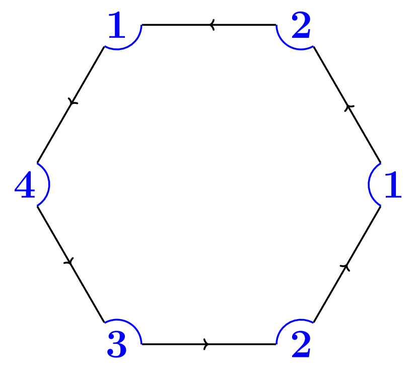
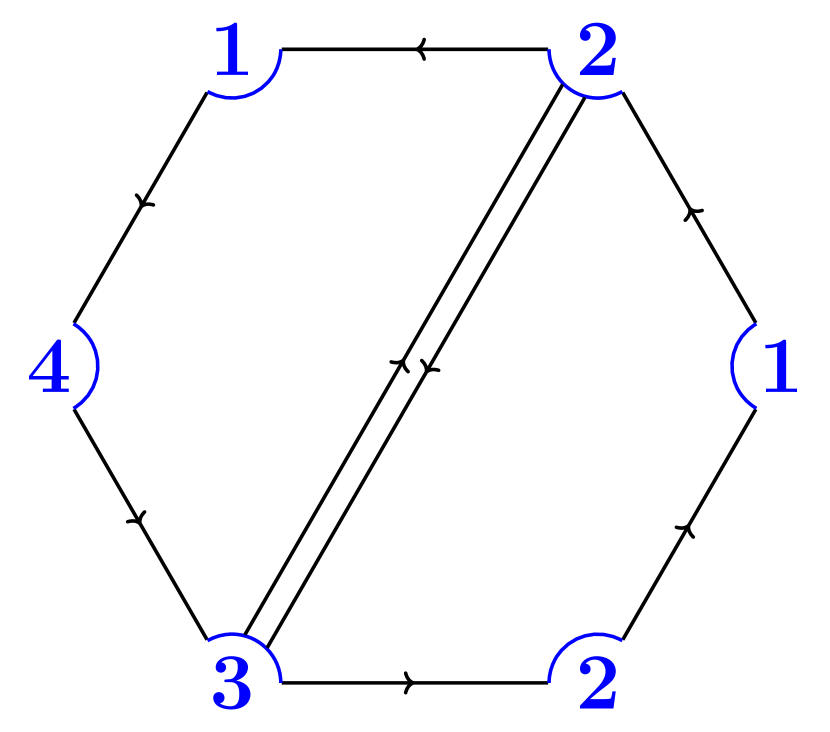
(a)	(b)

Figure 7: All bigger polygons, such as the hexagon shown in (a), can be split into squares by adding further bridges, as shown in (b). Adding such bridges does not increase the genus of the surrounding graph.

Note that we cannot break the squares into triangles, since each operator $\mathcal{O}_{i}$ can only connect to operators $\mathcal{O}_{i\pm 1}$. The squares in the last two lines of (2.2) only contain at most three different BPS operators and are thus protected by supersymmetry and simply give $1$. The square in the first line is the non-trivial function $\mathbb{O}$ that appeared already at genus zero.

To summarize, all graphs that contribute at genus $g$ in the large-$k$ limit are quadrangulations of a genus-$g$ surface, such that all faces are squares of the types (2.2). By Euler counting we have

$$2-2g=(V=4)+(F=n)-(E=4n/2)=4-n\,,$$ (2.3)

so that at genus $g$, all graphs contain a total of $n=2g+2$ squares and twice as many edges. Indeed, our single genus-zero skeleton graph was simply given by two squares, as explained in the previous section. In the three genus-one examples of Figure 3, we have four squares. It is also simple to see that the number of non-BPS squares $\mathbb{O}$ in each graph ought to be even. Therefore, we conclude that at each fixed genus $g$, all contributions sum to a polynomial $P_{g+1}$ in $\mathbb{O}^{2}$ of degree $g+1$, thus leading to (1.4). Finding these polynomials is tantamount to counting quadrangulations.

In order to count quadrangulations of surfaces of genus $g$ with $4$ vertices (punctures) and $2g+2$ squares, we introduce a matrix model. The matrix model naturally describes the duals of the skeleton graphs, where each of the $2g+2$ original square faces becomes a quartic vertex, and where the original $4$ vertex operators $\mathcal{O}_{1},\dots,\mathcal{O}_{4}$ become four faces of the dual graph. Each bridge connecting operators $\mathcal{O}_{i}$ with $\mathcal{O}_{i+1}$ is now pierced by a propagator of the dual graph; since there are four types of bridges $\mathcal{O}_{i}{-}\mathcal{O}_{i+1}$, we will have four complex matrices, one for each such original bridge type. See Figure 8 for the vertices and Figure 9 for example graphs with their duals.

Figure 8: Matrix model vertices. Each is the dual counterpart of the corresponding three square types represented in Figure 6.

Figure 9: Example graphs at genus $g=0,1,2$ (top) with their duals (bottom). In the top row we have four vertices (the BPS operators) and $2g+2$ faces (the squares). In the bottom row we have four faces (the BPS operators) and $2g+2$ quartic vertices (the squares).

There are $10$ different square faces in (2.2), and so there will be $10$ different vertices in the matrix model. All in all, the partition function of our matrix model is

$$Z\equiv\int[\mathcal{D}A][\mathcal{D}B][\mathcal{D}C][\mathcal{D}D]\exp\bigl{(}-S_{\text{kin}}[A,B,C,D]+S_{\text{int}}[A,B,C,D]\bigr{)}\,,$$ (2.4)

with the kinetic action term

$$S_{\text{kin}}=\operatorname{tr}\left[\frac{A\bar{A}}{k_{1}}+\frac{B\bar{B}}{k_{2}}+\frac{C\bar{C}}{k_{3}}+\frac{D\bar{D}}{k_{4}}\right]$$ (2.5)

and the interaction term

$$S_{\text{int}} =\mathbb{O}\operatorname{tr}(ABCD)+\mathbb{O}\operatorname{tr}(\bar{D}\bar{C}\bar{B}\bar{A})$$ (2.6)

$$+\operatorname{tr}\left[\frac{(A\bar{A})^{2}+(B\bar{B})^{2}+(C\bar{C})^{2}+(D\bar{D})^{2}}{2}+AB\bar{B}\bar{A}+BC\bar{C}\bar{B}+CD\bar{D}\bar{C}+DA\bar{A}\bar{D}\right]\,.$$

The interaction part consists of two non-BPS vertices in the first line (the duals of the non-BPS squares, which therefore come with a factor $\mathbb{O}$), and eight BPS vertices (which come with a factor of $1$ since they are BPS) in the second line.

In the kinetic term, we have introduced parameters $k_{i}$, $i=1,\dots,4$ as a means of counting the number of propagator bundles connecting $\mathcal{O}_{i}$ and $\mathcal{O}_{i+1}$ in each skeleton graph by simply reading off the corresponding power of $k_{i}$. This is quite important, because we have to dress each quadrangulation by four factors of the type (2.1), one for each type of connection. Keeping track of the numbers of different types of edges individually also allows us to calculate the correlator of a more general and considerably richer set of operators (the sum over permutations for $\mathcal{O}_{1}$ and $\mathcal{O}_{3}$ is implicit)

$$\mathcal{O}_{1}=\operatorname{tr}(\bar{Z}^{k_{4}}\,{\color[rgb]{1,0,0}\bar{X}}^{k_{1}}),\quad\mathcal{O}_{2}=\operatorname{tr}({\color[rgb]{1,0,0}X}^{k_{1}+k_{2}}\,),\quad\mathcal{O}_{3}=\operatorname{tr}(\bar{Z}^{k_{3}}\,{\color[rgb]{1,0,0}\bar{X}}^{k_{2}}),\quad\mathcal{O}_{4}=\operatorname{tr}({Z}^{k_{3}+k_{4}}).$$ (2.7)

At genus zero, there is again a single graph contributing to the correlator, and it is again a nice rectangle frame as in Figure 1(a). The difference is that now there are $k_{i}$ propagators connecting $\mathcal{O}_{i}$ and $\mathcal{O}_{i+1}$. The limit of large charges now amounts to taking all the $k_{i}$ to be of order $\sqrt{N_{\text{c}}}$. At genus zero, for example, we have

$$\langle\mathcal{O}_{1}\dots\mathcal{O}_{4}\rangle_{g=0}=\frac{{\color[rgb]{0,0,1}\mathbb{O}^{2}}}{(x_{1}-x_{2})^{2k_{1}}(x_{2}-x_{3})^{2k_{2}}(x_{3}-x_{4})^{2k_{3}}(x_{4}-x_{1})^{2k_{4}}}\,.$$ (2.8)

At higher genus, in the large charge limit and with $\mafx@zeta_{i}\equiv k_{i}/\sqrt{N_{\text{c}}}$,

$$\frac{\langle\mathcal{O}_{1}\dots\mathcal{O}_{4}\rangle}{\langle\mathcal{O}_{1}\dots\mathcal{O}_{4}\rangle_{\mafx@lambda=0,g=0}}\xrightarrow{\;k_{i}\sim\sqrt{N_{\text{c}}}\;}\sum_{g=0}^{\infty}\frac{P_{4g|g+1}(k_{1},k_{2},k_{3},k_{4},\mathbb{O}^{2})}{N_{\text{c}}^{2g}}\equiv\mathcal{A}(\mafx@zeta_{1},\mafx@zeta_{2},\mafx@zeta_{3},\mafx@zeta_{4},\mathbb{O})\,,$$ (2.9)

where $P_{4g|g+1}$ are polynomials of degree $g+1$ in $\mathbb{O}^{2}$ whose coefficients are homogeneous polynomials of degree $4g$ in the four $k_{i}$. When all $k_{i}$ are equal, then

$$P_{4g|g+1}(k_{i}|\mathbb{O}^{2})\xrightarrow{\,k_{i}\to k\,}k^{4g}P_{g+1}(\mathbb{O}^{2})\,,$$ (2.10)

and we get back to our previous correlator (1.4).

To obtain the full correlator (2.9) at genus $g$ from the matrix model (2.4), we bring down $2g+2$ vertices, pick the $N^{4}$ coefficient (since we are after a four-point correlation function, which in terms of the dual matrix model means that we are interested in graphs with four faces), and focus on those contributions where all $k_{j}$ appear. That last condition is due to R-charge conservation, which implies that all types of bridges between operators $\mathcal{O}_{i}$ and $\mathcal{O}_{i+1}$ must appear. We thus discard any monomials such as $k_{1}^{2}k_{2}^{2}$ which do not contain all $k_{i}$. All in all, the term that we are interested in is

$$Z=\dots+{\color[rgb]{0,0,1}N^{4}k_{1}k_{2}k_{3}k_{4}\Bigl{(}\mathcal{Z}\equiv\sum_{g=0}^{\infty}\tilde{P}_{4g|g+1}(k_{1},k_{2},k_{3},k_{4}|\mathbb{O}^{2})\Bigr{)}}+\dots$$ (2.11)

These tilded polynomials $\tilde{P}_{4g|g+1}$ count our quadrangulations, and are thus almost the polynomials arising in the correlator (2.9). To get precisely those, however, we also need to include the combinatorial factors (2.1). Since we strip out an overall $k_{1},\dots,k_{4}$ factor in defining the reduced partition function $\mathcal{Z}$, we finally conclude that

$$P_{4g|g+1}(k_{1},k_{2},k_{3},k_{4}|\mathbb{O}^{2})=\tilde{P}_{4g|g+1}(k_{1},k_{2},k_{3},k_{4}|\mathbb{O}^{2})\bigg{|}_{\displaystyle k_{1}^{n_{1}}\dots k_{4}^{n_{4}}\to\frac{k_{1}^{n_{1}}\dots k_{4}^{n_{4}}}{n_{1}!\dots n_{4}!}\,.}$$ (2.12)

or equivalently

$$\mathcal{A}(\mafx@zeta_{1},\mafx@zeta_{2},\mafx@zeta_{3},\mafx@zeta_{4},\mathbb{O})=\mathcal{Z}\big{|}_{k_{i}^{n}\to{\mafx@zeta_{i}^{n}}/{n!}}$$ (2.13)

for the full correlator at any genus and any coupling. This is our main result.

As a trivial check, consider genus zero. We need to bring down $2g+2=2$ vertices, i. e. we consider terms in the expansion of $\exp\left(-S_{\text{int}}\right)$ that are of degree $2$ in the interaction vertices. If we bring down two vertices from the second line in (2.6), we see right away that we either get more than four faces (from $\langle\operatorname{tr}(AB\bar{B}\bar{A})\operatorname{tr}(CD\bar{D}\bar{C})\rangle$ for example) or we generate terms which do not contain all $k_{i}$’s (from $\langle\operatorname{tr}(A\bar{A})^{2}\operatorname{tr}(B\bar{B})^{2}\rangle$ for example). Bringing down an odd number of vertices from the first line in (2.6) gives a zero result by charge conservation. So we are left with the possibility of bringing down two non-BPS vertices from the first line. This leads to

$$\mathbb{O}^{2}\langle\operatorname{tr}(ABCD)\operatorname{tr}(\bar{D}\bar{C}\bar{B}\bar{A})\rangle=N^{4}k_{1}k_{2}k_{3}k_{4}{\color[rgb]{0,0,1}\mathbb{O}^{2}}\,,$$ (2.14)

recognizing precisely the genus zero result in (2.8).

Bringing down further octagon vertices from $\exp\left(-S_{\text{int}}\right)$, we generate all the above-mentioned polynomials $\tilde{P}$ and thus their transformed partners $P$, which enter the four-point correlation function (2.9). We managed to compute the general polynomials $P_{4g|g+1}$ up to genus $g=4$. As we saw above, the genus-zero polynomial is simply $P_{0|1}=\mathbb{O}^{2}$. At genus one, we find

$$P_{4|2} =k_{1}k_{2}k_{3}k_{4}\left[1+\mathbb{O}^{2}\frac{\sum_{j=1}^{4}[(k_{j}+k_{j+1})^{4}-k_{j}^{4}]+12(k_{1}k_{2}+k_{3}k_{4})(k_{1}k_{4}+k_{2}k_{3})}{24k_{1}k_{2}k_{3}k_{4}}+\frac{\mathbb{O}^{4}}{2}\right].$$

The polynomials for $g=2,3,4$ are attached in the file polynomials.m. For equal charges, $k_{i}\equiv k$, the polynomials $P_{4g|g+1}$ reduce to $k^{4g}$ times a polynomial $P_{g+1}$ in $\mathbb{O}$ with rational coefficients, see (2.10). The resulting correlator $\mathcal{A}$ is quoted in (4.4) below. We have cross-checked the polynomials $P_{4g|g+1}$ obtained from the matrix model against an explicit construction of all contributing skeleton graphs up to genus three, see Appendix A.

Let us make three comments. The first one is that we are extracting the term with 4 faces, proportional to $N^{4}$. This is actually the smallest power of $N$ arising in the perturbative expansion if we keep only terms containing all four $k_{i}$, as we are instructed to do. (It would be the next-to-smallest if we lift the latter restriction.) This is in stark contrast with the usual large-$N$ expansion, where the leading terms carry the largest powers of $N$. So the limit we are interested in is a sort of $N\to 0$ limit of the matrix model.

In vector models, the limit of small number of colors is a very interesting one, related to polymers and other such fascinating combinatorics, see e. g. [20, 21, 22]. Another interesting instance of such limits shows up in the study of entanglement entropy and quenches disorder, where one often uses the replica trick to study the $n$ copies of a given system in the formal $n\to 0$ limit. This is done to generate logarithms (of a density matrix or partition function) that were originally absent through the identity $\lim_{n\to 0}(x^{n}-1)/n=\log(x)$. Sometimes the coupling between the various copies is encoded in a matrix, see e. g. [23, 24, 25]. In those cases, we are also interested in a formal limit where the matrix size goes to zero. Such matrices, present most notably in spin-glass studies, have extremely rich dynamics. In matrix model theory, dualities between $N\to\infty$ and $\tilde{N}\to 0$ limits have in fact been found before, in the context of the theory of intersection numbers of moduli spaces of curves, see [26, 27, 28, 29]. As we will see below, the $N\to 0$ limit will show up again and again in several simplified matrix model combinatorics in very amusing ways. It would be interesting to find a nice statistical mechanics application of this zero-color limit.

A second small comment is that we can consider rectangular matrices [31], where matrix $A$ has dimensions $N_{1}\times N_{2}$, matrix $B$ has dimensions $N_{2}\times N_{3}$, and so on. Then $N^{4}$ would be replaced by $N_{1}N_{2}N_{3}N_{4}$, identifying precisely the four faces corresponding to the four distinct operators. The terms containing this factor automatically contain all $k_{i}$, so using rectangular matrices would allow us to condense the instructions above into simply

$$\mathcal{Z}(k_{i})=\frac{1}{k_{1}k_{2}k_{3}k_{4}}\lim_{N_{i}\to 0}\frac{\partial}{\partial N_{1}}\frac{\partial}{\partial N_{2}}\frac{\partial}{\partial N_{3}}\frac{\partial}{\partial N_{4}}Z(N_{i},k_{i})\,.$$ (2.15)

This highlights once more the limit of small number of colors we are interested in.

The last comment pertains to the combinatorial replacement in (2.12). In effect, by introducing an extra $1/n!$ for each coupling $k_{i}^{n}$, we are Borel transforming our matrix model perturbative expansion. Interestingly, it renders the partition function expansion finite, as we will see explicitly below. Namely, the transformation removes the usual $(2g)!$ divergence that is due to the proliferation of graphs at higher genus [32, 33], and thus leads to a fully convergent expansion. While getting rid of divergences might be seen as a feature, losing the D-brane physics they encode is bit of a bug. This is presumably related to the fact that although we are resumming a ’t Hooft expansion, we are not generating arbitrarily complicated multi-string intermediate states. The large-charge limit projects onto folded strings, BMN strings and copies thereof, eliminating non-perturbative effects arising from the more complicated multi-string states which the D-branes source. It would be fascinating to slowly decrease the size of our BPS operators to move away from our fully convergent limit and carefully isolate these novel effects in a controllable way.

3 Matrix Model Simplification and Limits

Ideally, we would like to determine the full correlation function $\mathcal{A}(\mafx@zeta_{1},\mafx@zeta_{2},\mafx@zeta_{3},\mafx@zeta_{4},\mathbb{O})$ by solving the matrix model (2.4). That would be equivalent to computing the polynomials $P_{4g|g+1}$ to all genus, which we have not succeeded thus far. What we did manage to do is to simplify this matrix model problem into an equivalent matrix model problem where we have two hermitian matrices $\mathbb{M}_{1}$, $\mathbb{M}_{2}$ and two complex matrices $\mathbb{X}$, $\mathbb{Y}$, with a non-diagonal propagator between $\mathbb{X}$ and $\mathbb{Y}$ equal to the octagon function $\mathbb{O}$, so that

$$\langle F\rangle\equiv\int[\mathcal{D}\mathbb{M}_{1}][\mathcal{D}\mathbb{M}_{2}][\mathcal{D}\mathbb{X}][\mathcal{D}\mathbb{Y}]F\exp\biggl{[}-\frac{1}{2}\operatorname{tr}\mathbb{M}_{1}^{2}-\frac{1}{2}\operatorname{tr}\mathbb{M}_{2}^{2}-\operatorname{tr}\begin{pmatrix}\mathbb{X}&\!\!\mathbb{Y}\end{pmatrix}\!\begin{pmatrix}1&\!\!\mathbb{O}\\ \mathbb{O}&\!\!1\end{pmatrix}^{\!-1}\!\!\begin{pmatrix}\bar{\mathbb{X}}\\ \bar{\mathbb{Y}}\end{pmatrix}\biggr{]}.$$ (3.1)

Then we have the rather compact expression

$$\mathcal{Z}=\frac{\left\langle\operatorname{tr}\log\left(\mathbb{I}-\frac{k_{2}}{\mathbb{I}-k_{2}\mathbb{M}_{2}}\bar{\mathbb{X}}\frac{k_{1}}{\mathbb{I}-k_{1}\mathbb{M}_{1}}\mathbb{X}\right)\operatorname{tr}\log\left(\mathbb{I}-\frac{k_{3}}{\mathbb{I}-k_{3}\mathbb{M}_{2}}\bar{\mathbb{Y}}\frac{k_{4}}{\mathbb{I}-k_{4}\mathbb{M}_{1}}\mathbb{Y}\right)\right\rangle_{\text{two faces}}}{k_{1}k_{2}k_{3}k_{4}}$$ (3.2)

for the reduced partition function, from which we can readily extract the correlator via (2.13). When expanding the logarithms in powers of $k$, we can drop all terms whose total power is not a multiple of four, since the latter are the terms that correspond to an even number of octagons as required (at genus $g$ we keep $4g+4$ powers of $k$). We also extract the coefficient of $N^{2}$, which is the smallest power of $N$ on the right hand side. So again, in this alternative matrix model formulation, we are after the $N\to 0$ limit. As a check, we can expand to leading order in $k$ to get

$$\mathcal{Z}=\langle\operatorname{tr}(\bar{\mathbb{X}}\mathbb{X})\operatorname{tr}(\bar{\mathbb{Y}}\mathbb{Y})\rangle_{\text{two faces}}+\mathcal{O}(k^{4})\,,$$ (3.3)

which evaluates to $\mathbb{O}^{2}$, since Wick contracting complex fields of the same type would lead to four faces, and since each off-diagonal propagator equals $\mathbb{O}$. This is exactly what we expect at genus zero.

The derivation of (3.2) follows the graphical manipulations in Appendix C.2. Technically, we open up all quartic vertices in (2.6) into pairs of cubic vertices using auxiliary fields as detailed in Appendix C.4. If done carefully, the resulting action is Gaussian in the original four complex matrices. Integrating them out then leads to (3.2). In particular, the logarithms arise from the complex matrix identity

$$\int[\mathcal{D}\mathbb{A}]e^{-\operatorname{tr}(\mathbb{A}.\mathbb{Q}.\bar{\mathbb{A}})}=(\det\mathbb{Q})^{-N}\,.$$ (3.4)

It is particularly nice that in these integrations we explicitly generate two such factors which automatically produce two factors of $N$. That is why in (3.2) we extract two faces only rather than four as in the original representation with four complex matrices. Technically, this renders the representation (3.2) quite powerful. Besides, there are less degrees of freedom as we went from four complex matrices to two complex and two hermitian.

More physically, we started with a matrix model with four complex matrices corresponding to the four types of consecutive propagators in our large cyclic operators. The four-point function of these four cyclic operators was mapped to a dual correlation function with four faces in the dual matrix model with matrices $A,B,C,D$. The two-point function with two faces in (3.2) is thus a hybrid representation, where two of the four operators are represented as vertices and the other two as faces, see Figure 26. See [34, 19], and also the very inspiring talk [35] for very similar (and often more general) dynamical graph dualities obtained by integrating-in and -out matrix fields.

In practice, we compute (3.2) by expanding out the expression to any desired monomial in the $k_{i}$ and then preforming the various free Wick contractions. We found it particularly convenient to Wick contract the complex matrices first and the hermitian matrices at the end. Once $\mathbb{X}$ and $\mathbb{Y}$ are integrated out, because of the alternating pattern in (3.2) it is easy to see that we generate products of traces containing either $U_{k_{1}}({\color[rgb]{1,0,0}\mathbb{M}_{1}})$ and $U_{k_{4}}({\color[rgb]{1,0,0}\mathbb{M}_{1}})$ or $U_{k_{2}}({\color[rgb]{0,0,1}\mathbb{M}_{2}})$ and $U_{k_{3}}({\color[rgb]{0,0,1}\mathbb{M}_{2}})$, but never both (here $U_{k}(M)\equiv k/(\mathbb{I}-kM)$). Expanding further the $U_{k}$ in terms of the fundamental Hermitian fields we conclude that our full reduced partition function is given by a sum of factorized one-matrix correlators,

$$\mathcal{Z}=\sum_{g=0}^{\infty}\sum_{n_{1},\dots,n^{\prime}_{M^{\prime}}}\mathbb{C}^{(g)}_{n_{1},\dots,n^{\prime}_{M^{\prime}}}\times\langle\operatorname{tr}(\mathbb{M}_{1}^{n_{1}})\dots\operatorname{tr}(\mathbb{M}_{1}^{n_{M}})\rangle_{\text{one face}}\times\langle\operatorname{tr}(\mathbb{M}_{2}^{n^{\prime}_{1}})\dots\operatorname{tr}(\mathbb{M}_{2}^{n^{\prime}_{M^{\prime}}})\rangle_{\text{one face}}\,.$$ (3.5)

In this sum, $n_{1}+\dots+n_{M}+n^{\prime}_{1}+\dots+n^{\prime}_{M^{\prime}}\leq 4g$, and the combinatorial factors $\mathbb{C}^{(g)}$ arising from integrating out the complex matrices $\mathbb{X}$ and $\mathbb{Y}$ are homogeneous polynomials of degree $4g$ in the $k_{j}$, with coefficients that are polynomials in $\mathbb{O}^{2}$ of maximally degree $g+1$. Importantly, note that because of the factorization in (3.5), each Hermitian correlator now has to be restricted to a single face, which is quite a bit simpler than the previous two-face problem in (3.2), which in turn was a considerable simplification over the initial four-face problem in (2.4).

In fact, the one-face problem was solved already in the first days of matrix models, see e. g. the discussion below equation (9) in [36], from which we readily get the generating function of all these multi-trace Hermitian matrix model single-face expectation values as

$$\Bigl{\langle}\exp{\sum\limits_{n=1}^{\infty}t_{n}\operatorname{tr}(\mathbb{M}^{n})}\Bigr{\rangle}_{\!\text{one face}}\\ =\sum_{j=1}^{\infty}\sum_{k=0}^{j-1}\frac{(2k+1)!!(2j-2k-3)!!}{2j(-1)^{k}}\Bigl{(}\frac{j-2k-1}{k+1/2}\sum_{r=0}^{2k}\bar{p}_{r}p_{2j-r}-\bar{p}_{2k+1}p_{2j-2k-1}\Bigr{)}\,,$$ (3.6)

where $p_{r}$, $\bar{p}_{r}$ are defined via the Schur polynomial identities

$$\sum\limits_{n=0}^{\infty}p_{n}z^{n}\equiv\exp\biggl{(}\sum\limits_{n=1}^{\infty}z^{n}t_{n}\biggr{)}\quad\text{and}\quad\sum\limits_{n=0}^{\infty}\bar{p}_{n}z^{n}\equiv\exp\biggl{(}-\sum\limits_{n=1}^{\infty}z^{n}t_{n}\biggr{)}\,.$$ (3.7)

Another beautiful representation follows from the single-face limit of [37], which gives

$$\Bigl{\langle}\exp{\sum\limits_{n=1}^{\infty}t_{n}(\mathbb{M}^{n})}\Bigr{\rangle}_{\text{\!\text{one face}}}=\Bigl{(}\exp{\sum\limits_{a,b=0}^{\infty}{\overbrace{abt_{a}t_{b}\frac{\partial}{\partial t_{a+b-2}}}^{\text{splitting}}+\overbrace{(a+b+2)t_{a+b+2}\frac{\partial}{\partial t_{a}}\frac{\partial}{\partial t_{b}}}^{\text{joining}}}}\Bigr{)}t_{0}\,,$$ (3.8)

where the differential operator can be though of as implementing fusion and fission of the various traces as one Wick-contracts all these correlators, see Figure 10. For general $N$, we would replace the $t_{0}$ at the end by $e^{Nt_{0}}$, and the $N^{F}$ coefficient in the final expansion would compute the $F$–face result; it is quite a huge simplification to simply linearize this exponent to get a single face in (3.8), as needed for our problem.

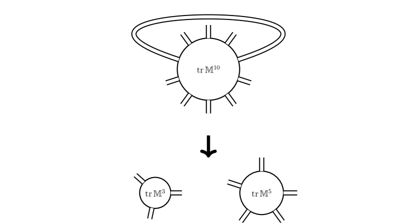
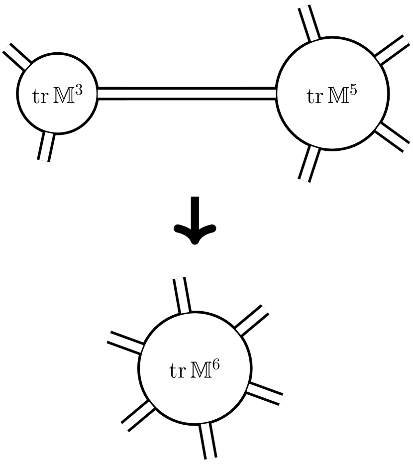
(a)	(b)

Figure 10: (a) Splitting and (b) joining of traces representend as differential operators in (3.8).

We could also try to integrate out the Hermitian matrices first.

This concludes the general description of our matrix model, and how we dealt with it in practice to produce higher-genus predictions. Next, we focus on interesting simplifying limits. There are at least three obvious interesting limits where our correlator should simplify:

$${\bf(A)}\,\,\mathbb{O}\to 1\,,\qquad{\bf(B)}\,\,\mathbb{O}\to 0\,,\qquad{\bf(C)}\,\,\mathbb{O}\to\infty\,.$$ (3.9)

The first corresponds to $\mafx@lambda=0$ or tree level (but all genus orders). The other limits are more interesting [39]. The second shows up, for example, at strong coupling, and also in interesting null limits at finite coupling. The last one would be realized for instance in the so-called bulk-point limit [40].

3.1 Small Octagon Limit, $\mathbb{O}\to 0$

In the small octagon limit where $\mathbb{O}\to 0$, we are left with the eight BPS square vertices in the second line of (2.6), all with the same weight $=1$. Now, there is another setup where we would have encountered these, and only these, type of vertices, namely if we were to study extremal correlators in the double-scaling limit of [4, 5, 6, 7, 8] using quadrangulations. There, we know how to solve the original problem directly, using single-matrix model technology, and the results found for these correlators are basically given by products of $\sinh(\mafx@omega_{ij}J_{i}J_{j})$ factors times some simple rational function, where $J_{i}$ are the charges of the involved operators, and the frequencies $\mafx@omega_{ij}$ are pure numbers. We cannot directly apply the very same techniques to our case, since we are now dealing with several complex matrices. Instead, we guessed that the result ought to take a similar form. We made an ansatz with a number of sinh factors and fixed the various frequencies and prefactors by matching with the first few terms of our matrix-model perturbative expansion. Then we computed a few more orders to cross-check the validity of this guess up to genus six. It all works out beautifully, and the result turns out to be remarkably simple:

$$\mathcal{A}(\mafx@zeta_{1},\mafx@zeta_{2},\mafx@zeta_{3},\mafx@zeta_{4}|\mathbb{O}=0)=\prod_{i=1}^{4}\,\frac{\sinh\left(\frac{1}{2}\,\mafx@zeta_{i}(\mafx@zeta_{i-1}+\mafx@zeta_{i}+\mafx@zeta_{i+1})\right)}{\frac{1}{2}\,(\mafx@zeta_{i-1}+\mafx@zeta_{i}+\mafx@zeta_{i+1})}\,.$$ (3.10)

In fact, we did a bit more than this: We considered a generalized matrix model, where each of the eight BPS vertices is dressed with an arbitrary coefficient, and guessed the general form of the resulting “twisted” correlator following the same strategy, see Appendix C.4. We also studied these generalized BPS quadrangulations for $n$-point extremal correlators in Appendix D.1, and for a setup where $n$ operators are cyclically connected (the correlator discussed here is the $n=4$ case of that) in Appendix D.2.

It would be very interesting to find a first-principle honest derivation of (3.10), starting from (2.4) or (3.1). It might very well elucidate powerful tricks which we may hope to use in the general case, where the octagon vertex is inserted back.

It is important to stress that the result (3.10) is very non-perturbative, although it has no coupling dependence in it. Note in particular that setting $\mathbb{O}\to 0$ is not the same as setting the coupling to zero, which is instead $\mathbb{O}\to 1$. When $\mathbb{O}\to 0$, the various loop corrections must work hard to completely cancel the tree-level result $\mathbb{O}=1$. For example, at genus zero and tree level, the correlator is equal to $1$, but it becomes $\mathbb{O}^{2}$ at non-zero coupling. So when $\mathbb{O}\to 0$, the full genus zero result is washed out non-perturbatively. In string terms, the BPS vertices describe point-like string configurations, while $\mathbb{O}$ describes a large folded string. When the string tension is very large, the BPS configurations with no area survive, while the big extended strings are suppressed. Recall that the planar result consists of just two copies of a big folded string glued together. Interestingly, this contribution gets suppressed for $\mathbb{O}\to 0$. At genus one, we start having configurations that are free of folded strings and those should survive. Indeed, the genus expansion of (3.10) starts at genus one:

$$\frac{\mathcal{A}}{k_{1}k_{2}k_{3}k_{4}} =0\times N_{\text{c}}^{0}\,+\,\frac{1}{N_{\text{c}}^{2}}+\frac{1}{N_{\text{c}}^{4}}\,\frac{1}{24}\sum_{j=1}^{4}k_{j}^{2}\left(k_{j-1}+k_{j}+k_{j+1}\right)^{2}$$

$$\qquad+\frac{1}{N_{\text{c}}^{6}}\frac{1}{1152}\,\sum_{i=1}^{4}\sum_{j=1}^{4}\left(1-{\textstyle\frac{2}{5}}\mafx@delta_{i,j}\right)k_{i}^{2}k_{j}^{2}(k_{i-1}+k_{i}+k_{i+1})^{2}(k_{j-1}+k_{j}+k_{j+1})^{2}$$

$$\qquad+\mathcal{O}(1/N_{\text{c}}^{8})$$ (3.11)

It would be cute if we could understand the numbers in this expansion directly from string theory by carefully counting these degenerate string configurations. A good starting point could be [41, 42], where degenerate point-like string configurations for two- and three- point functions were analyzed, see also [43, 44]. It would be interesting to generalize them to our BPS squares, and to understand how those can be put together purely in string terms.

3.2 Large Octagon Limit, $\mathbb{O}\to\infty$

Another interesting limit is the regime where the octagon $\mathbb{O}$ becomes very large. In this case, only the maximal power of $\mathbb{O}$ survives at each order in the genus expansion, which is $\mathbb{O}^{2g+2}$. In other words, we only use the two non-BPS squares in our quadrangulations, and set all BPS squares to zero. This dramatically simplifies the representation (3.2) to

$$\mathcal{Z}=\sum_{n=1}^{\infty}\frac{(k_{1}k_{2}k_{3}k_{4})^{n-1}\mathbb{O}^{2n}}{n^{2}}\langle\operatorname{tr}((\mathbb{X}\mathbb{Y})^{n})\operatorname{tr}((\bar{\mathbb{X}}\bar{\mathbb{Y}})^{n})\rangle_{\text{two faces}}\,,$$ (3.12)

where $\mathbb{X}$ and $\mathbb{Y}$ here are complex matrices with diagonal propagator normalized to $1$, i. e. with kinetic term simply given by $-\operatorname{tr}(\mathbb{X}\bar{\mathbb{X}})-\operatorname{tr}(\mathbb{Y}\bar{\mathbb{Y}})$. To arrive at this expression, we notice that (i) we can set to zero all $\mathbb{M}_{j}$ matrices, since they describe BPS quadrangulations, and (ii) we only keep the off-diagonal Wick contractions between the complex matrices in (3.2), since those generate octagons, while self-contractions do not. Since we are only off-diagonally contracting $\mathbb{X}$ with $\bar{\mathbb{Y}}$ and $\mathbb{Y}$ with $\bar{\mathbb{X}}$, we can swap $\bar{\mathbb{Y}}$ and $\bar{\mathbb{X}}$ and replace the off-diagonal by a purely diagonal propagator equal to $\mathbb{O}$ for the matrices $\mathbb{X}$ and $\mathbb{Y}$. Finally, we can rescale the propagator to $1$ by taking all factors of $\mathbb{O}$ out of the correlator. In this way, upon expanding the logarithms, we obtain (3.12).

The representation (3.12) immediately leads to a very compact expression for our correlator in the large octagon limit, since the dependence on $k$ is explicit, and thus the Borel-transform procedure can be done straightforwardly, yielding

$$\mathcal{A}=\frac{1}{\mafx@zeta_{1}\mafx@zeta_{2}\mafx@zeta_{3}\mafx@zeta_{4}}\sum_{n=1}^{\infty}\frac{(\mafx@zeta_{1}\mafx@zeta_{2}\mafx@zeta_{3}\mafx@zeta_{4}\mathbb{O}^{2})^{n}}{n^{2}\,{\color[rgb]{1,0,0}(n-1)!^{4}}}\langle\operatorname{tr}((\mathbb{X}\mathbb{Y})^{n})\operatorname{tr}((\bar{\mathbb{X}}\bar{\mathbb{Y}})^{n})\rangle_{\text{two faces}}\,.$$ (3.13)

The two-point function in this expression can be evaluated analytically at any $N$, that is for any number of faces, starting from its single-complex-matrix counterpart

$$\langle\operatorname{tr}(\mathbb{X}^{n})\operatorname{tr}(\bar{\mathbb{X}}^{n})\rangle=\sum_{k=1}^{n}\prod_{i=1}^{k}(i+N-1)\prod_{m=1}^{n-k}(N-m)\,.$$ (3.14)

This expression is derived by decomposing each trace into characters of hook representations (generating one sum per trace) and then using character two-point function orthogonality, thus killing one of the two sums. See for instance formula (B.2) in [6]. The final sum over hooks is (3.14). We want the same expression with $\mathbb{X}\to\mathbb{X}\mathbb{Y}$. To find it, we proceed as for the single-matrix case, except that we use so-called fission relations (see e. g. [45]) to open up characters $\mafx@chi_{\mafx@lambda}(\mathbb{X}\mathbb{Y})$ into $\mafx@chi_{\mafx@lambda}(\mathbb{X})\mafx@chi_{\mafx@lambda}(\mathbb{Y})$ upon doing the relative matrix angle integral between the two matrices. Each character thus splits into two, so the representation (3.14) ends up being modified to

$$\left\langle\operatorname{tr}((\mathbb{X}\mathbb{Y})^{n})\operatorname{tr}((\bar{\mathbb{X}}\bar{\mathbb{Y}})^{n})\right\rangle=\sum_{k=1}^{n}\left(\prod_{i=1}^{k}(i+N-1)\prod_{m=1}^{n-k}(N-m)\right)^{\color[rgb]{1,0,0}\!2}\,.$$ (3.15)

We can now simply expand the summand at small $N$ to read off the leading $N\to 0$ term, which is precisely the required two-face contribution. Plugging that into (3.13), we obtain our full correlator

$$\mathcal{A}=\frac{1}{\mafx@zeta_{1}\mafx@zeta_{2}\mafx@zeta_{3}\mafx@zeta_{4}}\sum_{g=0}^{\infty}\frac{(\mafx@zeta_{1}\mafx@zeta_{2}\mafx@zeta_{3}\mafx@zeta_{4}\mathbb{O}^{2})^{g+1}}{(g+1)^{2}\,{g!^{4}}}\sum_{m=0}^{g}m!^{2}(g-m)!^{2}\,.$$ (3.16)

We can re-sum this expression into

$$\mathcal{A}=\mathbb{O}^{2}\int\limits_{0}^{1}ds\int\limits_{0}^{1}dt\left[\frac{s\,t}{s+t-1}\,I_{0}\bigl{(}2\sqrt{s\,t\,\mafx@omega}\bigr{)}-\frac{(1-s)(1-t)}{s+t-1}\,I_{0}\bigl{(}2\sqrt{(1-s)(1-t)\,\mafx@omega}\bigr{)}\right]\,,$$ (3.17)

where $\mafx@omega=\mafx@zeta_{1}\mafx@zeta_{2}\mafx@zeta_{3}\mafx@zeta_{4}\mathbb{O}^{2}$, and where $I_{0}$ is the modified Bessel function of the first kind. Note that this expression is valid for $\mathbb{O}$ large, $k_{j}$ large, $N_{\text{c}}$ large, but $\mafx@omega=k_{1}k_{2}k_{3}k_{4}\mathbb{O}^{2}/N_{\text{c}}^{2}$ can be either large or not, it depends on how these limits are taken. In particular we find

$$\mathcal{A}\simeq\frac{1}{\mafx@zeta_{1}\mafx@zeta_{2}\mafx@zeta_{3}\mafx@zeta_{4}}\times\begin{cases}\mafx@omega+O(\mafx@omega^{2})&\mafx@omega\ll 1\,,\\[8.53581pt] \displaystyle\frac{e^{2\sqrt{\mafx@omega}}}{\sqrt{\mafx@pi}\,\mafx@omega^{1/4}}&\mafx@omega\gg 1\,.\end{cases}$$ (3.18)

As mentioned above, in the two-point function representation (3.2), each of the two logarithms represents one of the large cyclic operators, and the two faces encode the remaining two operators. This is how this matrix model representation encodes our original four-point correlator. There are other representations of this fully non-BPS result, which are instructive in their own right, such as the original matrix model where the four operators are faces, and also two new representations in Appendix C.3: A one-point function with three faces, and a three-point function with one face, see (C.15). In all these matrix model representations, we are after the leading term in the $N\to 0$ limit.

Finally, let us stress once more the very important effect of the Borel $1/g!$ arising from the large operator combinatorics. It is the four $1/g!$ factors in (3.16) that are responsible for the very nice convergence of this expression. Indeed,

$$\sum_{m=0}^{g}m!^{2}(g-m)!^{2}\simeq 2(g!)^{2}\simeq\sqrt{4\mafx@pi g}\,4^{-g}\,(2g)!\qquad\text{for}\qquad g\gg 1\,,$$ (3.19)

exhibiting the usual large-genus behavior expected in such string/matrix theories [32, 33]. This growth would otherwise render the matrix model perturbative expansion asymptotic, with missing non-perturbative effects hinting at the physics of D-branes, see above. Because of the extra combinatorial factors in (3.16) we obtain instead a perfectly convergent expression (3.17) with asymptotic behavior (3.18).

3.3 Free Octagon Limit, $\mathbb{O}\to 1$

Having analyzed the very non-perturbative $\mathbb{O}\to 0$ and $\mathbb{O}\to\infty$ limits, we turn to what should naively be a much simpler limit: The free octagon limit, where $\mathbb{O}\to 1$. In this case, the diagonal and off-diagonal propagators of the complex matrices in (3.2) are identical. Hence the matrices $\mathbb{X}$ and $\mathbb{Y}$ can be identified, thus leading to a simpler matrix model representation with a single complex matrix $\mathbb{X}$ and two Hermitian matrices $\mathbb{M}_{1}$ and $\mathbb{M}_{2}$, with partition function

$$\mathcal{Z}=\frac{\left\langle\operatorname{tr}\log\left(\mathbb{I}-\frac{k_{2}}{\mathbb{I}-k_{2}\mathbb{M}_{2}}\bar{\mathbb{X}}\frac{k_{1}}{\mathbb{I}-k_{1}\mathbb{M}_{1}}\mathbb{X}\right)\operatorname{tr}\log\left(\mathbb{I}-\frac{k_{3}}{\mathbb{I}-k_{3}\mathbb{M}_{2}}\bar{\mathbb{X}}\frac{k_{4}}{\mathbb{I}-k_{4}\mathbb{M}_{1}}\mathbb{X}\right)\right\rangle_{\text{two faces, }k^{4m}}}{k_{1}k_{2}k_{3}k_{4}}\,,$$ (3.20)

where

$$\langle F\rangle\equiv\int[\mathcal{D}\mathbb{M}_{1}][\mathcal{D}\mathbb{M}_{2}][\mathcal{D}\mathbb{X}]F\exp\Bigl{[}\frac{1}{2}\operatorname{tr}\mathbb{M}_{1}^{2}+\frac{1}{2}\operatorname{tr}\mathbb{M}_{2}^{2}+\operatorname{tr}\mathbb{X}\bar{\mathbb{X}}\Bigr{]}\,.$$ (3.21)

Once Borel transformed, this matrix model partition function computes the tree level correlator ($\mafx@lambda=0$) of the operators (2.7) at any genus order in the double-scaling limit where $k_{j}/\sqrt{N_{\text{c}}}$ is held fixed with $k_{j}$ and $N_{\text{c}}$ both taken to infinity. As before, it is easy to expand this correlator to very high genus order. However, compared to the previous cases, we were not able to either derive or guess the all-genus expansion. It would be very interesting to find the proper matrix model technology allowing us to compute the expectation value (3.20) in this amusing $N\to 0$ limit where the two-face contribution dominates.

Perhaps we could even expect more, and actually compute the correlator for any $N_{\text{c}}$ in this free theory limit. Note that the space-time dependence at tree level is completely fixed by R-charge conservation and thus factors out, as there must be exactly $k_{i}$ propagators connecting each two consecutive operators. The free-theory all-genus correlator is thus given by a matrix model of two complex matrices that are simply the complex scalars $Z$ and $X$ in $\mathcal{N}=4$ SYM. Perhaps this model can be solved using two-matrix model techniques following e. g. [46, 47, 48, 49].

A related observation stemming from the absence of any non-trivial space-time dependence at tree level, and from the fact that complex fields cannot self-contract, is that the free-theory correlator can also be though of as a two-point function of a holomorphic double-trace operator $\mathcal{O}=\operatorname{tr}({X}^{k_{1}+k_{2}}\,)\operatorname{tr}({Z}^{k_{3}+k_{4}})$ with an anti-holomorphic double trace operator $\mathcal{O}^{\prime}=\operatorname{tr}(\bar{Z}^{k_{4}}\,{\bar{X}}^{k_{1}})\operatorname{tr}(\bar{Z}^{k_{3}}\,{\bar{X}}^{k_{2}})$. If we could decompose these operators into restricted Schur polynomials as in [50, 51], we could exploit their orthogonality to evaluate the free correlator at finite $N_{\text{c}}$ and $k_{i}$.

Another final option would be to try to compute the free correlator for many more values of $k_{i}$ and $N_{\text{c}}$, observe a pattern and guess the full result.

4 Conclusions

In this work, we considered the four-point function

$$\frac{\langle{\operatorname{tr}({\color[rgb]{0,0,0}\mafx@mathbold{\bar{Z}}^{k}}{\color[rgb]{1,0,0}\mafx@mathbold{\bar{X}}^{k}})(0)}\,{\operatorname{tr}({\color[rgb]{1,0,0}\mafx@mathbold{X}^{2k}})(z)}\,{\operatorname{tr}({\color[rgb]{1,0,0}\bar{\mafx@mathbold{X}}^{k}}{\color[rgb]{0,0,0}\mafx@mathbold{\bar{Z}}^{k}})(1)}\,{\operatorname{tr}({\mafx@mathbold{Z}^{2k}})(\infty)}\rangle}{\text{same at $\mafx@lambda=0$ and $\text{genus}=0$}}\equiv\mathcal{A}(\mafx@zeta|\mathbb{O})$$ (4.1)

in the double-scaling limit where $N_{\text{c}}$ and $k$ are both very large with

$$\mafx@zeta=\frac{k}{\sqrt{N_{\text{c}}}}$$ (4.2)

held fixed. This correlator $\mathcal{A}(\mafx@zeta|\mathbb{O})$ is very rich, but still simple enough that we can say a great deal about it, and often even about its all-genus re-summation.

The reason for this is a nice decoupling of the large $N_{\text{c}}$ expansion combinatorics – which are encoded in the dependence of the function $\mathcal{A}$ on the effective coupling $\mafx@zeta$ and on the octagon function $\mathbb{O}$ – and the finite ’t Hooft coupling dynamics and conformal field theory geometry – which enter through the octagon function alone as $\mathbb{O}=\mathbb{O}(z,\bar{z}|\mafx@lambda)$. We deal with the very interesting dynamics of $\mathbb{O}$ in [39], while here we attacked the combinatorial problem. In fact, the separation of combinatorics and dynamics relies on nothing but a little bit of supersymmetry, on the large $N_{\text{c}}$ limit, and on having large $R$-charges to play with. We should therefore be able to find octagons and perform very similar – if not identical – re-summations in other gauge theories with less supersymmetry.

We found for instance that as $\mathbb{O}\to 0$, the correlator (4.1) simplifies to

$$\mathcal{A}=\left(\frac{\sinh(\frac{3}{2}\mafx@zeta^{2})}{\frac{3}{2}\mafx@zeta}\right)^{4}\,,$$ (4.3)

while as $\mathbb{O}\gg 1$, we obtain instead

$$\mathcal{A} =\mathbb{O}^{2}\int\limits_{0}^{1}dt\int\limits_{0}^{1}ds\,\left[\frac{ts}{t+s-1}\,I_{0}\bigl{(}2\sqrt{t\,s}\,\mafx@zeta^{2}\mathbb{O}\bigr{)}-\frac{(1-t)(1-s)}{t+s-1}\,I_{0}\bigl{(}2\sqrt{(1-t)(1-s)}\,\mafx@zeta^{2}\mathbb{O}\bigr{)}\right].$$ (4.4)

For general finite $\mathbb{O}$, we could compute the function $\mathcal{A}$ through genus four, i. e. as a Taylor expansion in $\mafx@zeta$ as

$$\mathcal{A}=\mathbb{O}^{2} +\mafx@zeta^{4}\left(1+{\textstyle\frac{9}{2}}\mathbb{O}^{2}+{\textstyle\frac{1}{2}}\mathbb{O}^{4}\right)$$

$$+\mafx@zeta^{8}\left({\textstyle\frac{3}{2}}+{\textstyle\frac{607}{80}}\mathbb{O}^{2}+{\textstyle\frac{97}{36}}\mathbb{O}^{4}+{\textstyle\frac{1}{16}}\mathbb{O}^{6}\right)$$

$$+\mafx@zeta^{12}\left({\textstyle\frac{81}{80}}+{\textstyle\frac{7321}{1120}}\mathbb{O}^{2}+{\textstyle\frac{953}{216}}\mathbb{O}^{4}+{\textstyle\frac{5689}{12960}}\mathbb{O}^{6}+{\textstyle\frac{5}{1296}}\mathbb{O}^{8}\right)$$

$$+\mafx@zeta^{16}\left({\textstyle\frac{459}{1120}}+{\textstyle\frac{75553}{22400}}\mathbb{O}^{2}+{\textstyle\frac{44971}{12600}}\mathbb{O}^{4}+{\textstyle\frac{5587171}{7257600}}\mathbb{O}^{6}+{\textstyle\frac{2903}{86400}}\mathbb{O}^{8}+{\textstyle\frac{31}{207360}}\mathbb{O}^{10}\right)$$

$$+\mathcal{O}(\mafx@zeta^{20})\,.$$ (4.5)

These are our main results. It would be formidable to find the full form of $\mathcal{A}$, interpolating between (4.3) and (4.4), and reproducing (4.5) in the ’t Hooft expansion. Obtaining one more simplifying point of data, such as the free correlator $\mathbb{O}\to 1$, might provide us with some inspired guess.

We conclude with some further comments on generalizations and future directions.

The hexagonalization prescription of [10, 11, 12, 13, 14, 15], or the octagonalization prescription for large operators described here, splits the study of correlators into a problem of combinatorics of skeleton graphs and the dynamics related to filling in the faces of these graphs by integrability-computed objects (octagons in our case). In the dual graph picture, we end up taming these skeleton graphs with matrix models with a small fixed number of faces that correspond to the vertices in our correlator, since graph duality interchanges vertices and faces. So we end up with matrix models where we are interested not in a large $N$ expansion of the matrix model – where the maximal number of faces dominate in the ’t Hooft expansion – but rather in the small $N\to 0$ limit, which projects onto the required correlators with a small number of faces. We developed some technology for dealing with this interesting $N\to 0$ limit whenever needed in our examples. Matrix model dualities between large/small matrix rank limits have been studied before in the context of intersection number theory [26, 27, 28, 29]. It would be fascinating to further explore the mathematics of these dualities, as well as their use in our context.

We dubbed our correlator as cyclic, because the R-charge polarizations of the operators are chosen such that operator $\mathcal{O}_{i}$ is forced to connect only to operators $\mathcal{O}_{i\pm 1}$. Since we have six scalars in $\mathcal{N}=4$ SYM, we can as well construct generalized cyclic configurations with five and with six operators (but not more), see Figure 11.

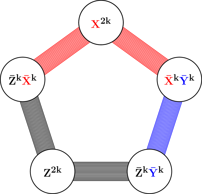
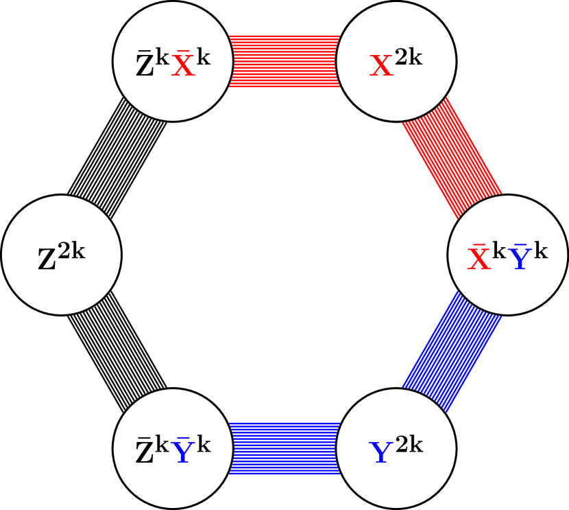
(a)	(b)

Figure 11: Polarized (a) five-point and (b) six-point functions

What happens to these higher cyclic correlators in the double scaling limit (4.2)? Again, because of the large charges, the contributing graphs will have to be maximal, which means that all faces are bounded by a minimal number of edges. However, contrary to the four-point case, the indivisible faces are not just squares (i. e. octagons). We now have non-BPS pentagons (for the five-point function) and non-BPS hexagons (for the six-point function) besides the various BPS squares (there are $10$/$12$ different BPS squares for the five/six point function). For a skeleton graph made of $n_{\text{s}}$ squares, $n_{\text{p}}$ pentagons, and $n_{\text{h}}$ hexagons, the number of edges is $n_{\text{e}}=(4n_{\text{s}}+5n_{\text{p}}+6n_{\text{h}})/2$. By Euler’s formula for $n$ vertices at genus $g$, we find for the number $n_{\text{e}}$ of edges

$$\frac{n_{\text{e}}}{2}=2g-2+n-\frac{n_{\text{p}}}{4}-\frac{n_{\text{h}}}{2}\,.$$ (4.6)

Hence maximizing the number of edges requires to saturate the tiling of the surface with squares only! That means that these correlators in the double-scaling (DS) limit actually have no coupling dependence, they are purely given by BPS quadrangulations, which we found in Appendix D.2. Explicitly, we find

$$\frac{G_{5}^{\text{DS}}}{G^{\text{DS}}_{\text{5,free,planar}}}=\left(\frac{\sinh(\frac{3}{2}\mafx@zeta^{2})}{\frac{3}{2}\mafx@zeta}\right)^{5}\,,\qquad\frac{G_{6}^{\text{DS}}}{G^{\text{DS}}_{\text{6,free,planar}}}=\left(\frac{\sinh(\frac{3}{2}\mafx@zeta^{2})}{\frac{3}{2}\mafx@zeta}\right)^{6}\,.$$ (4.7)

Of course, we could look for subleading corrections to the double-scaling limit where interesting coupling dependence would show up. This would be particularly interesting for the six-point case, since we expect the non-BPS hexagon – being akin to a four-dimensional six-point function – to probe the genuine bulk-point singularity in four dimensions [40].

We could also consider non-cyclic operators, and in particular maximally connected configurations where all operators share propagators with all others. Here, the relevant maximal graphs will be BPS triangulations, and the relevant scaling would be $k\sim N_{\text{c}}^{1/3}$. It would be nice to consider this limit and the corresponding matrix model.

In this last example, as well as in the previous five-point and six-point cyclic function examples, we end up with tessellations where all building blocks are BPS polygons with trivial expectation value $=1$. We expect them to become interesting functions of the coupling as we twist the theory, thus breaking supersymmetry. An extreme and very interesting example to analyze would be the fish-net deformation [52, 53], whose hexagons have been introduced in [54, 55].

It is common to think of the sums over skeleton graphs in hexagonalization and octagonalization prescriptions as some sort of discretization of the string moduli space [10, 15]. The picture could be slightly different in a string-bit-like description, as recently put forward in the context of $\mathrm{AdS}_{5}\times\mathrm{S}^{5}$ strings in [56], and in the fish-net theory in [57]. In [56], for instance, the underlying theory is topological, and the sum over ways of connecting the various string bits could perhaps be identified with the summation over the various skeleton graphs. It would be nice to see the hexagons and octagons more explicitly in the language of these works.

Everything so far was about very large operators. Can we go beyond the large-operator limit and construct a dual matrix model formulation of $\mathcal{N}=4$ SYM, with hexagons as vertex building blocks describing any correlation function at any genus and any coupling? In a way, it would be a concrete gauge theory realization of the very inspiring proposal [58]. All our dreams can come true, if we have the courage to pursue them, said Walt Disney. So we should try.

Appendix A Constructing Graphs Explicitly

In the following, we want to explicitly construct all skeleton graphs up to a given genus. Listing the explicit graphs will allow us to compute the polynomials $P_{4g|g+1}(k_{1},k_{2},k_{3},k_{4})$ entering the correlator (2.9), and hence will provide an important cross-check of the results obtained with the help of matrix model techniques in Section 2 and Section 3. Moreover, constructing all contributing graphs explicitly is of more general interest: In the present paper, we consider the case where all bridges (propagator bundles) contain a large number of propagators, such that all faces are isolated from each other (the sum over mirror excitations / open string states reduces to the vacuum / ground state). Hence for the purpose of this paper, it is sufficient to know the number of graphs that can be formed from a given set of faces; how exactly these faces are arranged in each individual graph is irrelevant. However, the more general hexagonalization prescription [10, 13, 14, 15] for finite-charge operators requires to include non-trivial states that propagate between faces, hence one does have to know the local structure of each graph explicitly. Hence it is important to have techniques to construct the relevant graphs.

Mathematically, the graphs that we need to construct are ribbon graphs (also called fat graphs). In short, a ribbon graph is an ordinary graph equipped with a cyclic ordering of the edges incident to each vertex. More precisely, an ordinary graph consists of a set $V$ of vertices, a set $H$ of half-edges, a map $s:H\to V$ that maps each half-edge to the vertex that it is incident on, and a map $i:H\to H$ (involutive, without fixed points) that maps each half-edge to its other half. A ribbon graph is an ordinary graph $(V,H,s,i)$ together with a bijection $\mafx@sigma:H\to H$ whose cycles correspond to the sets $s^{-1}(v)$ of half-edges incident on vertices $v\in V$. The ordering of each cycle prescribes the ordering of the incident half-edges at the vertex $v$. Topologically, each vertex of a ribbon graph can be thought of as a disk, and each edge as a narrow rectangle (or “ribbon”, hence the name “ribbon graph”) attached to two of the vertex disks. The boundaries of these ribbons together with segments of the vertex disks naturally form the faces of a ribbon graph (each face bounded by $n$ ribbons is a cycle of $(i\circ\mafx@sigma)^{\circ n}$). Inserting an open disk into each of these faces completes every ribbon graph to a compact oriented surface with a definite genus, which we call the genus of the graph.

For our purposes, each vertex represents a single-trace operator, and we think of it as a disk whose perimeter is formed by the ordered fields within the trace. Each edge of a ribbon graph represents a bundle of parallel propagators that connect a number of adjacent fields within the single traces of the two operators connected by the edge. We will alternatively call the edges “propagator bundles” or “bridges”, depending on context. Because they are propagators, and because our operators are local, we exclude edges that connect an operator to itself. Also, we exclude “parallel” edges that connect to identical operators next to each other (in a planar fashion): Since the edges represent bundles of parallel propagators, such parallel edges could be merged into a single edge (in the above language, such parallel edges would form cycles of $i\circ\mafx@sigma\circ i\circ\mafx@sigma$). Hence we only consider graphs where all faces are bounded by at least three edges.

To summarize, we want to consider ribbon graphs with $n$ vertices (punctures) of a given genus, ruling out edges that connect any vertex to itself, and demanding that all faces are bounded by at least three edges, i. e. all faces are triangles or bigger polygons. In the following, we call ribbon graphs with these properties just “graphs”. We are particularly interested in graphs that are complete in the sense that no further edge can be added to them (without increasing the genus). We call such graphs maximal graphs. Obviously, every graph can be promoted to a maximal graph by adding bridges. Hence conversely, every graph can be obtained from some maximal graph by deleting edges. For this reason, we shall focus on constructing the complete set of maximal graphs at a given genus.

It is easy to see that all faces of maximal graphs are either triangles or squares. All bigger polygons can be split into smaller polygons by inserting further bridges. But squares whose diagonally opposite vertices are identical cannot be split, because we exclude edges that connect any vertex to itself. Hence every face in a maximal graph is either a triangle touching three different vertices, or a square whose diagonally opposite vertices are identical. By imagining fictitious edges that also split all squares into triangles, we can think of every maximal graph of genus $g$ as a triangulation of a genus-$g$ surface.

A given triangulation of a Riemann surface can be transformed into a different triangulation by flipping some of its edges, where flipping an edge means the transformation

$$\text{I}:\qquad\includegraphics[align=c]{FigFlipruleIleft.mps}\quad\longrightarrow\quad\includegraphics[align=c]{FigFlipruleIright.mps}\,.$$ (A.1)

Here, the circles are the vertices, and we have labeled them arbitrarily. Now, it is a mathematical theorem that the space of triangulations of a surface of fixed genus and with a given number of punctures is connected under the action of flipping edges (see e. g. [59]). In other words, any two triangulations are related by a sequence of edge flips. This means that, starting with any single triangulation, one can obtain all other triangulations by iteratively flipping edges. Since we can associate a triangulation to every maximal graph, we can also obtain all maximal graphs from a single maximal graph by flipping edges. This requires flipping real edges as well as fictitious edges that we added in order to split all squares into triangles. However, we can shortcut the introduction of fictitious edges by supplementing the flip operation (A.1) with further transformations that operate on squares. Namely, when an edge separates a triangle and a square, we have to consider the following transformation:

$$\text{II}:\qquad\includegraphics[align=c]{FigFlipruleIIleft.mps}\quad\longrightarrow\quad\includegraphics[align=c]{FigFlipruleIIright.mps}\,.$$ (A.2)

Here, the labels are again arbitrary, but their distribution is unique. An edge may also separate two squares. Such edges can be transformed in two inequivalent ways, and we have to include both of them:

$$\text{III}:\qquad\includegraphics[align=c]{FigFlipruleIIIleft.mps}\quad\longrightarrow\quad\left\{\,\includegraphics[align=c]{FigFlipruleIIIright1.mps}\,,\;\includegraphics[align=c]{FigFlipruleIIIright2.mps}\,\right\}\,.$$ (A.3)

The flip move (A.2) cannot be undone by iterations of move I without introducing self-contractions. In order to exhaust the space of maximal graphs, we thus also need to include the inverse of (A.2):

$$\text{IV}:\qquad\includegraphics[align=c]{FigFlipruleIIright.mps}\quad\longrightarrow\quad\includegraphics[align=c]{FigFlipruleIIleft.mps}\,.$$ (A.4)

Again, the labels are arbitrary, but their distribution matters and is unique. Each of the transformations II–IV is the result of a sequence of simple flip moves (A.1) acting on real as well as fictitious bridges (that split the squares). By the above considerations, it is clear that the complete set of maximal graphs at a given genus can be obtained by starting with an arbitrary maximal graph and iterating the operations (A.1)–(A.4) in all possible ways.

The result of the above discussion is the following iterative algorithm that constructs all maximal graphs at a given genus:

1. Start with any maximal graph of the desired genus. This can for example be constructed by iteratively adding random edges to the empty graph until the target genus is reached, and then splitting all faces of the resulting graph with as many further edges as possible.

2. For each edge of each graph in the list constructed in the previous iteration step, generate a new graph by applying one of the transformations (A.1)–(A.3) to that edge (transformation III generates two new graphs). For each pair of adjacent edges with vertex structure as in (A.4), generate a new graph by applying transformation IV.

3. The list of graphs constructed in the previous step may contain graphs that are identical to graphs constructed in earlier iteration steps. It can also contain several copies of identical graphs. Drop all graphs that are identical to graphs already constructed earlier, and drop all duplicates. The resulting list contains the new graphs.

4. Iterate steps 2–3 until the list of new graphs is empty, i. e. until all edge transformations only generate copies of graphs already found earlier.

We can implement this algorithm on a computer, and construct the space of maximal graphs for various genera and numbers of insertions (vertices). In order to reduce overcounting, we treat all vertices as identical, i. e. we use unlabeled vertices. The size of the space of graphs grows rapidly, see Table 1.

		genus
		$0$	$1$	$2$	$3$	$4$
number of insertions	$2$ :	$1$	$1$	$4$	$82$	$7325$
	$3$ :	$1$	$3$	$38$	$661$
	$4$ :	$2$	$16$	$760$	$122307$
	$5$ :	$4$	$132$	$18993$
	$6$ :	$14$	$1571$	$487293$
	$7$ :	$66$	$20465$
	$8$ :	$409$	$278905$
	$9$ :	$3078$
	$10$ :	$26044$

Table 1: Numbers of maximal graphs for various genera and numbers of insertions. Here, the vertices of the graphs are unlabeled, i. e. all vertices are treated as identical.

We note the following properties of maximal graphs of genus $g$ with $n$ vertices:

• The planar two-point graph has one edge.

• For $g=0$ and $n\geq 3$, all maximal graphs consist of $2n-4$ triangles and no squares, they have $3n-6$ edges.

• For $g\geq 1$ and $n=2$, all maximal graphs consist of $2g$ squares and no triangles, they have $4g$ edges.

• For $g\geq 1$ and $n\geq 3$, maximal graphs may consist of triangles and squares, their maximum edge number is $6g+3n-6$ (no squares, $2n+4g-4$ triangles), and their minimum edge number is $4g+3n-7$ ($2g+1$ squares, $2n-6$ triangles).

A note on the implementation: We found it convenient to represent ribbon graphs as lists of vertices, where each vertex is an ordered list of incident edges. For example, the graphs on the left in Figure 9 can be represented in Mathematica as

⬇

graph[v[1,2], v[1,3], v[2,4], v[3,4]]

graph[v[1,2,3], v[1,4,2,5,6], v[3,7,8], v[4,8,5,6,7]]

graph[v[1,2,3,4,5,6], v[1,7,8,3,9,10,5], v[2,4,11,6,12], v[7,11,8,9,12,10]]

Here, the edges have been given arbitrary integer labels. The bijection $\mafx@sigma$ is explicit in this representation, whereas the incidence and half-edge identification maps $s$ and $i$ are implicit. Of course, graphs in this representation are separately invariant under (i) permuting the vertices v[..] within graph[..], (ii) rotating the edge labels within individual vertices v[..], and (iii) relabeling the edges. When checking for equality of two graphs, these invariances have to be taken into account. A brute-force way of canonicalizing the representation is to tabulate over all permutations of the vertices v[..] as well as over all possible rotations of the edge labels within each vertex, enumerating the edges in order of appearance in each of the resulting representations, and to select the lexicographically smallest representative of the set.

Now that we have obtained all maximal graphs at a given genus, it is easy to construct all graphs of that genus by iteratively removing bridges in all possible ways, taking care to drop duplicate graphs at each step. In particular, it is straightforward to obtain all graphs that contribute to the four-point correlator (2.9). Namely, the contributing graphs still have a maximal number of edges, but now under the constraint that $\mathcal{O}_{i}$ only connects to $\mathcal{O}_{i\pm 1}$, but not to $\mathcal{O}_{i+2}$ (mod $4$). In other words, the four vertices of the graph have to split into two pairs, where the members of each pair are not connected by any edge. We call such graphs maximal cyclic graphs. To find them, we can take our list of maximal four-point graphs, group the four vertices into pairs in all (three) possible ways, and delete all edges connecting the members of each pair. Some of the resulting graphs will not be maximal, those have to be dropped (in practice, this can be done by keeping only graphs with $4g+4$ edges). Following this procedure, we find $6$, $215$, and $26779$ maximal cyclic graphs at genus $1$, $2$, and $3$, respectively, which we attach in the file maxcycgraphs.m

Armed with these lists of maximal cyclic graphs, we can now construct the polynomials $P_{4g|g+1}$. Since we have treated all vertices as identical (unlabeled) thus far, we first have to sum over all inequivalent vertex labelings for each unlabeled graph. In addition, each labeled graph comes with combinatorial factors from summing over all ways of distributing the propagators on all edges (bridges) of the graph. According to (2.1), summing over the distribution of $k_{i}$ propagators on $b_{i}$ bridges results in a factor $k_{i}^{b_{i}-1}/(b_{i}-1)!$. Hence each labeled graph comes with a combinatorial factor

$$\prod_{i=1}^{4}\frac{k_{i}^{b_{i}-1}}{(b_{i}-1)!}\,,$$ (A.5)

where $b_{i}$ is the number of edges (bridges) connecting vertices (operators) $\mathcal{O}_{i}$ and $\mathcal{O}_{i+1}$ (mod $4$) in the given graph.

There is one more point that we need to take into account: When we organize the sum over all Wick contractions into a sum over skeleton graphs and a sum over distributions of propagators on the edges of those skeleton graphs, it may happen that two or more seemingly different distributions of propagators on the same skeleton graph may actually represent identical Wick contractions. The reason for this is that we implicitly treat all edges as distinguishable (i. e. labeled) when we perform the sum over distributions of propagators. In particular, this assumption is implicit in the counting (2.1) leading to (A.5), therefore resulting in an overcounting that we have to compensate. At the level of skeleton graphs, this overcounting manifests itself in terms of non-trivial ribbon graph automorphisms. Such automorphisms are defined as follows: In a given ribbon graph (with unlabeled vertices and edges), temporarily pick unique labels for all vertices and edges, and mark a fixed point on the perimeter of each of the vertices, in between any two adjacent incident edges. There are many different possible positions for these marked points. A non-trivial automorphism is a combination of edge and vertex relabelings that transform the graph with any other choice of marked points to the same graph with the previously fixed chosen positions of marked points. The set of automorphisms for a given ribbon graph $\mafx@Gamma$ form the automorphism group $\operatorname{Aut}\mafx@Gamma$. This group does not depend on the initially chosen positions of marked points. In order to compensate the overcounting explained above, one has to divide the propagator-distribution factor (A.5) by the size $|\operatorname{Aut}\mafx@Gamma|$ of the automorphism group. We find $(1,3,24)$ graphs with $|\operatorname{Aut}\mafx@Gamma|=2$ at genus $(1,2,3)$, two graphs with $|\operatorname{Aut}\mafx@Gamma|=3$ at genus two, and three graphs with $|\operatorname{Aut}\mafx@Gamma|=4$ at genus three. All other graphs up to genus three have trivial automorphism group.

Now all that remains is to count within each graph $\mafx@Gamma$ the number $p(\mafx@Gamma)$ of faces that touch all four vertices. Each of these faces will be home to one octagon function $\mathbb{O}$, see (2.2). To construct the desired polynomials $P_{4g|g+1}$, we have to sum over the set $\mafx@mathbold{\mafx@Gamma}_{g}$ of all maximal cyclic ribbon graphs of genus $g$ with four vertices, and, for each graph $\mafx@Gamma\in\mafx@mathbold{\mafx@Gamma}_{g}$, over all inequivalent ways $\ell$ of assigning the operators $\mathcal{O}_{i}$, $i=1,\dots,4$ to the four vertices. The polynomials then are

$$P_{4g|g+1}=\sum_{\mafx@Gamma\in\mafx@mathbold{\mafx@Gamma}_{g}}\frac{1}{|\operatorname{Aut}\mafx@Gamma|}\sum_{\ell}\prod_{i=1}^{4}\frac{k_{i}^{b_{i}(\mafx@Gamma_{\ell})-1}}{(b_{i}(\mafx@Gamma_{\ell})-1)!}\,\mathbb{O}^{p(\mafx@Gamma)}\,.$$ (A.6)

Here, $b_{i}(\mafx@Gamma_{\ell})$ is the number of edges connecting vertices (operators) $\mathcal{O}_{i}$ and $\mathcal{O}_{i+1}$ in the labeled graph $\mafx@Gamma_{\ell}$. This concludes the construction of the polynomials $P_{4g|g+1}$ from explicit graphs. We computed these polynomials up to $g=3$ in this way, and found a perfect match with the polynomials computed with matrix-model techniques as explained in Section 2 and Section 3.

Appendix B From Minimal to Maximal Graphs

In this appendix we present a complementary approach to that of Appendix A on the construction of skeleton graphs. We propose to start by finding the minimal graphs which are graphs with a single face or minimum number of edges for given fixed genus $g$ and number of vertices $n$. Using these as a seed we can find all other graphs by adding new edges recursively such that we do not change the genus of the original graphs. This procedure stops when we saturate the graphs, such that any additional edge would change the genus. This final stage corresponds to the maximal graphs described in the previous appendix.

A graph with a fixed number of vertices $n$ and genus $g$ is minimal when it has a single face. From the Euler formula it follows that it also has the minimum number of edges

$$2-2g=(F_{\text{min}}=1)+(V=n)-E_{\text{min}}\quad\to\quad E_{\text{min}}=n+2g-1$$ (B.1)

An instance of a minimal graph with four punctures and genus one is presented in Figure 12.

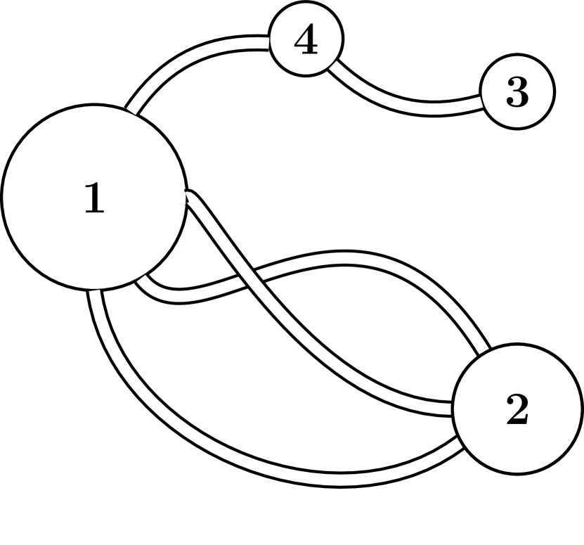
Figure 12: Minimal graph example with $n=4$ and $g=1$.

Another useful way of representing a minimal graph is given in Figure 13 (a), where we present the single face of the graph as a polygon whose sides represent the $2E_{\text{min}}$ half-edges (these are of the form $1\rightarrow 2$ and $2\leftarrow 1$ which reconstruct an edge $1\rightleftharpoons 2$ in the fat graph), and its vertices given by partitions of the original punctures of the graph. This latter representation allows us to recognize that a minimal graph can be found by starting with a $(2E_{\text{min}})$-gon and identifying its edges in a pairwise fashion such that we encapsulate $n$ vertices or punctures. In more detail we follow these steps to construct the minimal graphs:

• We start with a polygon with $2E_{\text{min}}$ sides and some orientation.

• We label the vertices with numbers from $1$ to $n$ in all possible ways, allowing for repetitions in order to cover all vertices, but we do not allow for neighboring vertices with the same label as this would represent a self-contraction that we must dismiss. If we consider special polarizations as in the main text, then we should also dismiss the polygons with pairs of neighboring vertices labeled by operators that cannot connect.

• For each of the labeled polygons generated in the previous step, we identify pairs of sides (half-edges) of the form $1\rightarrow 2$ and $1\leftarrow 2$ to reconstruct the edges of the graph $1\rightleftharpoons 2$. By doing so, all the vertices of the polygon with the same label also get together to reconstruct a puncture with that given label in the graph. We obtain a consistent graph when we get a total of $n$ punctures with labels from $1$ to $n$, with no repetition.

An alternative to this procedure can be found in the space of dual graphs, where we trade faces by vertices. The dual of a minimal graph has a single vertex, $E_{\text{min}}$ edges, and $n$ faces. The advantage is that all these dual $n$-faced dual graphs can be found from Wick contractions in the Gaussian one-point function of a Hermitian matrix $\langle\operatorname{tr}(\mathbb{M}^{2E_{\text{min}}})\rangle$. For instance see Figure 13 (b), each Wick contraction there tells us how to identify the sides of the polygon in Figure 13 (a). This dual point of view also facilitates the counting of the minimal graphs as nicely explained in [18] and derived in [60]. However the counting in those references has to be adapted to include labels in order to apply to the counting of our minimal graphs. We do not pursue this here, as our aim is only to provide a way to construct the minimal graphs.

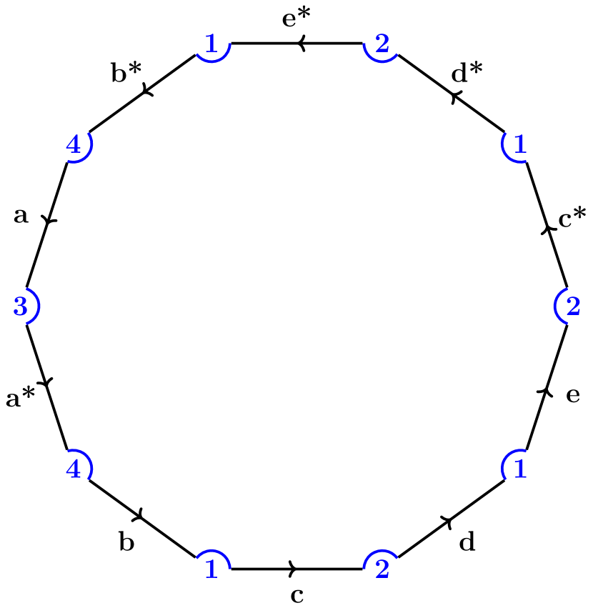
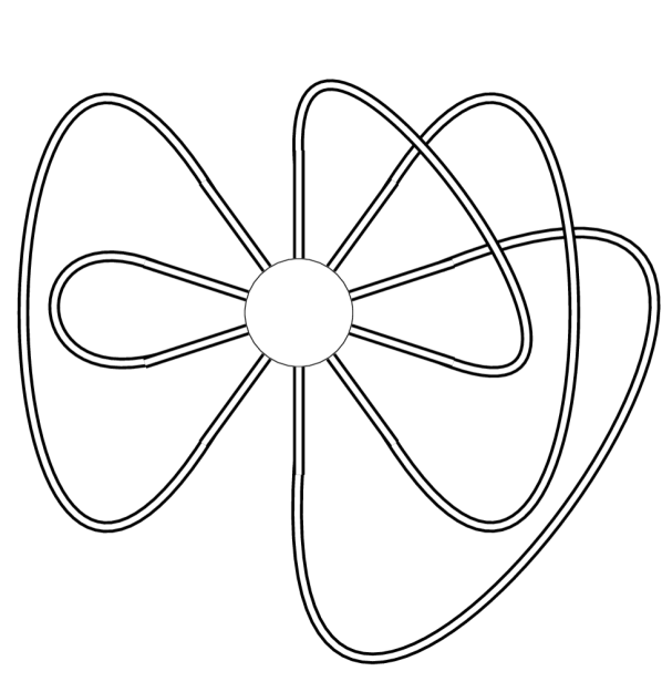
(a)	(b)

Figure 13: The genus-one minimal graph of Figure 12 represented as the polygon of its single face (a), and its dual represented by Wick contractions in a one-point matrix correlator (b).

Skeleton graphs with a higher number of edges can be simply constructed by adding edges to the minimal graphs. We would like to maintain the genus, so each additional edge must increase the number of faces by one to satisfy the Euler formula

$$2-2g=(1+F_{\text{add}})-n+(E_{\text{min}}+E_{\text{add}})\quad\Rightarrow\quad F_{\text{add}}=E_{\text{add}}\,.$$ (B.2)

To achieve this we simply start with the polygon representing a minimal graph, and consider the additional edges as non-intersecting diagonals of the polygon. These divide the polygon into sub-polygons which represent the faces of the new non-minimal graphs.

Furthermore, we should only allow for diagonals that connect vertices of the polygon with different labels, otherwise we would be including self-connections. In the case of special polarizations, as considered in the main body of this paper, we should also disallow diagonals representing prohibited connections.

Adding non-intersecting diagonals one by one to each polygon of a minimal graph, we generate all skeleton graphs. In general the saturation of the number of edges happens when we turn on all possible non-intersecting diagonals forming a triangulation of the polygon of a minimal graph, see Figure 14 (a). From this consideration it follows that the maximum number of edges and faces a maximal graph can have are

$$E_{\text{max}} =(E_{\text{min}}=n+2g-1)+(E_{\text{add}}=2E_{\text{min}}-3)=3(E_{\text{min}}-1)$$

$$=3\,(n+2g-2)\,,$$ (B.3)

$$F_{\text{max}} =2E_{\text{min}}-2=2\,(n+2g-2)\,,$$ (B.4)

where the additional number of edges $E_{\text{add}}$ simply corresponds to the maximal number of non-intersecting diagonals in the $(2E_{\text{min}})$-gon and the maximum number of faces $F_{\text{max}}$ is the number of triangles.

Due to the restriction of no self-connections, the saturation of edges can also happen before we reach the maximum value of edges (B). This is the case for the maximal graph in Figure 14 (b) represented by a tessellation containing both triangular and square faces.

In order to find all maximal graphs, we need to find all ways of triangulating the polygons of the minimal graphs. This can be achieved by following a recursive procedure of bifurcation of polygons. Performing this procedure, we generate the list of all maximal graphs starting with the minimal graphs as a seed. We obtained results up to genus $3$ which confirm the maximal graph generating algorithm of Appendix A. The disadvantage is that the final list of graphs is redundant, since some originally different minimal graphs get identified after adding new edges. In practice we noticed that we only need to consider triangulations of relatively few minimal graphs to obtain the full list of maximal graphs. It would be nice to better understand how to single out a minimal subset of all minimal graphs that generates all maximal graphs.

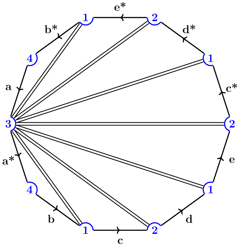
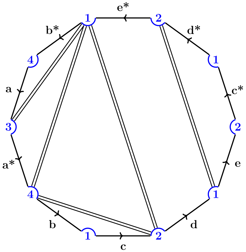
(a)	(b)

Figure 14: Genus One: A maximal skeleton graph with only triangular faces (a), and an edge-saturated skeleton graph with triangular and square faces (b).

Appendix C Counting Quadrangulations Including Couplings

C.1 Introduction

For the correlator studied in this paper we have specific polarizations that restrict the connections to be only between neighbors $1-2-3-4-1$. This condition dismisses triangles, so we only need to consider squares to find the corresponding maximal graphs that dominate in the double scaling limit (DSL) considered in the main text.

In Figure 15 (a) we present a genus-one quandrangulation obtained from the minimal graph of Figure 13 (a) by adding non-intersecting charged-allowed diagonals only, or from the (truly) maximal graph in Figure 14 (a) by erasing the charge-disallowed connections $1-3$ and $2-4$.

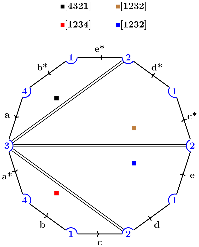
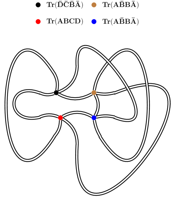
(a)	(b)

Figure 15: A genus-one quadrangulation and its graph dual as Wick contractions of four-valent vertices.

The squares entering a quadrangulation of our correlator can be classified according to the labels (operators 1,2,3 or 4) at its vertices. We have three types of squares as presented in (2.2) and in Figure 16. The first type includes the non-BPS squares $[1234]$ and $[4321]$ that evaluate to $1$ in the free theory, and to the octagon function $\mathbb{O}$ when the coupling is turned on. The other two types are BPS squares of them form $[abcb]$ and the other four of form $[abab]$. These latter squares still evaluate to $1$ when turning on the coupling.

Figure 16: The three types of squares that enter a quadrangulation. The vertices denote the punctures.

Figure 17: The three types of squares that enter a quadrangulation. The original vertices $1,2,3,4$ are now faces tha lie between the new edges.

In order to find the graph’s form by gluing these squares, we prefer to work in the dual space, where these faces are traded by four-valent vertices, see Figure 17. In this dual space, we have a total of 10 vertices, which define a matrix model with action

$$S =\,-\operatorname{tr}A\bar{A}-\,\operatorname{tr}B\bar{B}-\,\operatorname{tr}C\bar{C}-\,\operatorname{tr}D\bar{D}+\mathbb{O}\,\left(\operatorname{tr}(ABCD)+\,\operatorname{tr}(\bar{D}\bar{C}\bar{B}\bar{A})\right)$$

$$\qquad+\frac{\mafx@alpha_{1}}{2}\,\operatorname{tr}(A\bar{A}A\bar{A})+\frac{\mafx@alpha_{2}}{2}\operatorname{tr}(B\bar{B}B\bar{B})+\frac{\mafx@alpha_{3}}{2}\operatorname{tr}(C\bar{C}C\bar{C})+\frac{\mafx@alpha_{4}}{2}\operatorname{tr}(D\bar{D}D\bar{D})$$

$$\qquad+\mafx@beta_{1}\,\operatorname{tr}(DA\bar{A}\bar{D})+\mafx@beta_{2}\,\operatorname{tr}(AB\bar{B}\bar{A})+\mafx@beta_{3}\,\operatorname{tr}(BC\bar{C}\bar{B})+\mafx@beta_{4}\,\operatorname{tr}(CD\bar{D}\bar{C})$$ (C.1)

Unlike the action in (2.6), which only includes the coupling $\mathbb{O}$ for non-BPS squares, here we include couplings associated to each four-valent vertex to distinguish each type of square. This gives the advantage of keeping track of the specific squares that form a quadrangulation, which can help recognizing symmetries or patterns essential for a genus resummation.

In this dual space, a quadrangulation is given by Wick contractions in a Gaussian correlator as represented in Figure 15 (b). The correlator of this particular set of (dual) vertices can be explicitly computed as:

$$\frac{1}{2!}\left\langle\operatorname{tr}(ABCD)\operatorname{tr}(\bar{D}\bar{C}\bar{B}\bar{A})\operatorname{tr}(AB\bar{B}\bar{A})^{2}\right\rangle=N^{4}+12N^{6}+\frac{9}{2}N^{8}+\frac{1}{2}N^{10}$$ (C.2)

On the left hand side we add a symmetry factor due to the two identical vertices in the correlator. The result on the right hand side is given as a polynomial in $N$, the rank of the complex matrices, and from the exponents we can read off the number of faces of the graphs constructed by Wick contractions. We are only interested in the four-faced graphs, as they give the original four operators when dualized back. Furthermore in order to guarantee the dualized four faces give four different operators, we must have all $A,B,C,D$ matrices present in our correlators of four-valent vertices.

The relevant 4-faced partition function, extracted from the matrix model with action (C.1), is explicitly given by

$$\mathbf{Z}(\mathbb{O},\mafx@alpha_{i},\mafx@beta_{i})=\sum_{g=0}^{\infty}\sum_{T_{g}=\{t_{1},\cdots t_{2g+2}\}\in V_{4}}\frac{1}{\text{\text{sym}($T_{g}$)}}\left\langle\prod_{m=1}^{2g+2}\,t_{m}\right\rangle_{4\text{ faces}}$$ (C.3)

where we use the notation $\langle\cdots\rangle_{4\text{ faces}}$ to indicate we extract the coefficient of $N^{4}$ only. The subset $T_{g}=\{t_{1},\cdots t_{2g+2}\}$ is a list of $2g+2$ vertices, which are picked from the list of ten four-valent vertices with couplings $V_{4}=\{\mathbb{O}\,\operatorname{tr}(ABCD),\cdots,\mafx@beta_{4}\,\operatorname{tr}(CD\bar{D}\bar{C})\}$ announced in (C.1), with the extra condition of containing all matrices $A,B,C,D$. The symmetry factor $\text{sym}(T_{g})$ contains a factor of $2$ for each vertex of the form $\operatorname{tr}(X\bar{X}X\bar{X})$ and a factor $n!$ when we have $n$ identical vertices $t_{m}$.

The partition functions $\mathbf{Z}$ of (C.3) and $\mathcal{Z}$ of (2.11) or (2.15) are identical up to a simple replacement of couplings:

$$k_{1}k_{2}k_{3}k_{4}\,\mathcal{Z}(\mathbb{O},k_{i})=\mathbf{Z}(\mathbb{O},\mafx@alpha_{i},\mafx@beta_{i})\big{|}_{\mafx@alpha_{i}\to k_{i}^{2},\,\mafx@beta_{i}\to k_{i-1}k_{i},\,\mathbb{O}^{2}\to\mathbb{O}^{2}k_{1}k_{2}k_{3}k_{4}}$$ (C.4)

As explained in Section 2, the partition function $\mathcal{Z}$ requires a Borel-type transformation to give the cyclic correlator $\mathcal{A}$, see (2.13) . The analog transformation for $\mathbf{Z}$ defines the partition function

$$\mathbf{A}=\sum_{g=0}^{\infty}\sum_{T_{g}=\{t_{1},\cdots t_{2g+2}\}\in V_{4}}\frac{1}{\text{\text{sym}($T_{g}$)}}\frac{1}{\text{weight}(T_{g})}\left\langle\prod_{i=1}^{2g+2}\,t_{i}\right\rangle_{4\text{ faces}}$$ (C.5)

where the sole difference with (C.3) is the inclusion of the factorials:

$$\text{weight}(T_{g})\,=\,(n_{A}-1)!(n_{B}-1)!(n_{C}-1)!(n_{D}-1)!$$ (C.6)

with $n_{X}$ counting the number of appereances of $X$ in the subset $T_{g}$ of $2g+2$ vertices. Notice by construction we always demand $n_{X}\geq 1$.

The partition function $\mathbf{A}$ of (C.5) is identified with the cyclic correlator $\mathcal{A}$ under the replacement

$$\mafx@zeta_{1}\mafx@zeta_{2}\mafx@zeta_{3}\mafx@zeta_{4}\,\mathcal{A}(\mathbb{O},\mafx@zeta_{i})=\mathbf{A}(\mathbb{O},\mafx@alpha_{i},\mafx@beta_{i})\big{|}_{\mafx@alpha_{i}\to\mafx@zeta_{i}^{2},\,\mafx@beta_{i}\to\mafx@zeta_{i-1}\mafx@zeta_{i},\,\mathbb{O}^{2}\to\mathbb{O}^{2}\mafx@zeta_{1}\mafx@zeta_{2}\mafx@zeta_{3}\mafx@zeta_{4}}$$ (C.7)

with $\mafx@zeta_{i}={k_{i}}/{\sqrt{N_{\text{c}}}}$.

By a direct computation of the correlators $\langle\cdots\rangle_{4\text{ faces}}$ in (C.5) we obtain, up to genus one:

$$\mathbf{A}(\mathbb{O},\mafx@alpha_{i},\mafx@beta_{i})=\mathbb{O}^{2}+\frac{1}{2}\mathbb{O}^{4}\\ +\mathbb{O}^{2}\left(\sum_{i=1}^{4}\left(\frac{1}{24}\mafx@alpha_{i}^{2}+\frac{1}{6}\mafx@alpha_{i}(\mafx@beta_{i}+\mafx@beta_{i+1})+\frac{1}{4}\mafx@beta_{i}^{2}\right)+\frac{1}{2}(\mafx@beta_{1}+\mafx@beta_{3})(\mafx@beta_{2}+\mafx@beta_{4})\right)+\mafx@beta_{1}\mafx@beta_{2}\mafx@beta_{3}\mafx@beta_{4}+\cdots$$ (C.8)

where the dots indicate contributions from genus two and higher. This latter expression can be compared with (4.5) under the replacement (C.7) and after setting $\mafx@zeta_{i}=\mafx@zeta$.

At higher genus, the correlators $\langle\cdots\rangle_{4\text{ faces}}$ become computationally more demanding, so in order to simplify them we use integrating-in and -out operations that we describe in the following section.

C.2 Graph Operations

In order to simplify the correlators $\langle\cdots\rangle_{4\text{ faces}}$ of four-valent vertices, we now introduce operations that reduce them to correlators with less number of faces. We will present these operations at the level of graphs, nevertheless they have an obvious translation into matrix theory language as integrating-in and -out matrix fields.

C.2.1 Integrating-In: Adding Edges

We use this operation to split a four-valent vertex into two three-valent vertices. This can be useful to restructure a graph and set it up for the application of other simplifying operations.

This operation is performed in two steps as shown in Figure 18. In the first step we introduce a new edge and increase the number of vertices by one, such that the genus of the graph is maintained. As shown in the middle column of Figure 18, there are two possibilities to add this intermediate edge. In this specific example the two different options require two different types of edges. The top type needs an edge with different faces on its sides and can be represented by a complex matrix in the matrix language. The bottom type needs an edge with the same face on its sides and can be represented by a Hermitian matrix. Finally in the second step we split this new edge resulting in two new three-valent vertices.

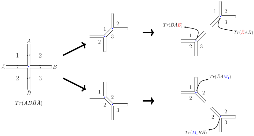
Figure 18: Adding an extra intermediate edge

Ultimately, we want to connect back the intermediate edge to reconstruct the graph. But typically, we will first perform other simplifications, such as integrating-out, before restoring the intermediate edge, such that the final result will be simpler than the original graph.

C.2.2 Integrating-Out: Removing A Face

We use this operation to decrease the number of faces, vertices and edges all at the same time, such that the genus of the graph does not change. In the matrix language, this corresponds to integrating out one or more matrix fields.

To perform this operation, we first choose a reference face, labeled by $1$ for instance. Then we organize all vertices that have a $1$ appearing between their edges around the reference face as shown on the left panel of Figure 19. The next step is to remove the reference face, such that all vertices on its perimeter get contracted to a single effective vertex that inherits all the outer edges, as shown on the right panel of Figure 19.

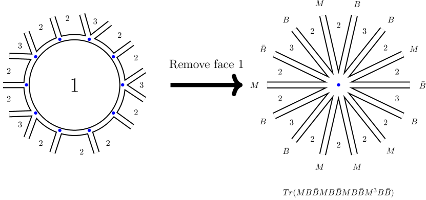
Figure 19: Vertices organize around a reference face

In some cases it is possible to choose more than one reference face, such that all vertices participate in an integrating-out operation. On the other hand, in some cases it is not possible to pick a reference face at first, for instance we can not place four-valent vertices with faces between edges $[1212]$ around a reference face $1$ or $2$. In these cases, making an integrating-in operation first can allow to organize the resulting vertices of lower valence around a reference face. In the following sections, we will perform combinations of these graph operations to simplify the counting of quadrangulations.

C.3 Non-BPS Quadrangulations

As a warm-up, we consider quadrangulations formed by squares $[1234]$ and $[4321]$ only. As described in the main text, this addresses the limit of large coupling $\mathbb{O}$. In the dual space, the relevant matrix model has action

$$S_{\text{large }\mathbb{O}}=\,-\operatorname{tr}A\bar{A}-\,\operatorname{tr}B\bar{B}-\,\operatorname{tr}C\bar{C}-\,\operatorname{tr}D\bar{D}+\mathbb{O}\,\left(\operatorname{tr}(ABCD)+\,\operatorname{tr}(\bar{D}\bar{C}\bar{B}\bar{A})\right)\,.$$ (C.9)

The simplicity of this problem allows for the application of different graph operations, which lead to different simplified outcomes. In what follows, we list some of these results, summarized in Section C.3.4.

C.3.1 As a 1-vertex and 3-faces problem

Having only vertices $\operatorname{tr}(ABCD)$ and $\operatorname{tr}(\bar{D}\bar{C}\bar{B}\bar{A})$, we can easily apply the integrating-out technique by picking as reference the face $1$ (or any of the other three). Then, as shown in Figure 20, there is a unique way of organizing the vertices on the perimeter of this reference face, that is alternating the two types of vertices. After removing the reference face $1$, the result is an effective vertex with fields $B$ and $C$ (and conjugates) only, the fields $A$ and $D$ are integrated out.

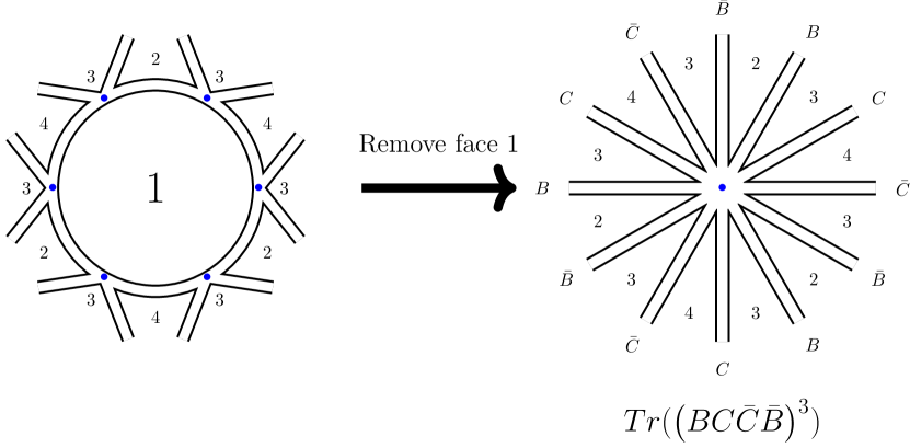
Figure 20: Genus-two example: The unique way of organizing the four-valent vertices around a reference face $1$, which leads to a single effective vertex, once we remove the reference face.

The non-BPS quadrangulations counted by the correlator of four-valent vertices $\langle\cdots\rangle_{4\text{ faces}}$ can now be counted by a one-point correlator $\langle\operatorname{tr}(\cdots)\rangle_{3\text{ faces}}$, see equation (C.13).

C.3.2 As a 2-vertices and 2-faces problem

Another simplification of the non-BPS counting can be achieved by first integrating-in complex fields in the non-BPS vertices as shown in figure Figure 21.

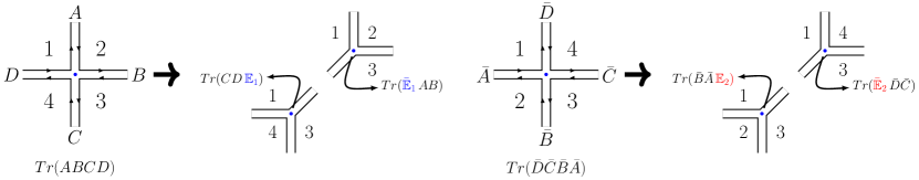
Figure 21: Splitting non-BPS vertices.

After splitting the four-valent vertices, we can arrange all three-valent vertices around two reference faces ($2$ and $4$) as shown in Figure 22.

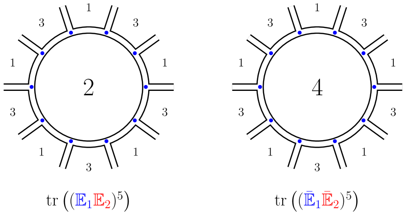
Figure 22: Genus four non-BPS example: Integrating out faces $2$ and $4$ gives a single two-point function of traces with two complex matrices.

Then we remove these faces $2$ and $4$, which effectively integrates out all $A,B,C,D$, and obtain two effective vertices that contain only the fields $\mathbb{E}_{1}$ and $\mathbb{E}_{2}$ (and conjugates). Now the quadrangulation counting can be found by computing a two-point function $\langle\operatorname{tr}(\cdots)\operatorname{tr}(\cdots)\rangle_{2\text{ faces}}$, see equation (C.14).

C.3.3 As a 3-vertices and 1-face problem

Naturally, dualizing the 1-vertex and 3-face problem, we obtain a 3-vertices and 1-face problem. We have not worked out in detail the necessary graph operations to get this latter outcome starting with the four-valent vertices. Nevertheless, by working out a few examples, we figured out what the correlator is, and present it in equation (C.15)

C.3.4 Summary for Non-BPS squares

We use $\mathcal{N}_{g}$ to denote the number of non-BPS quadrangulations weighted by their corresponding symmetry factors (automorphisms). From genus $g=0$ to $g=5$ these numbers, not necessarily integers, are:

$$\{\mathcal{N}_{g}\}=\{1,\frac{1}{2},1,5,\frac{248}{5},840,\cdots\}$$ (C.10)

they appear in the large $\mathbb{O}$ limit of $\mathcal{A}$, see (3.12), as:

$$\mathcal{A}=\frac{1}{\mafx@zeta_{1}\mafx@zeta_{2}\mafx@zeta_{3}\mafx@zeta_{4}}\sum_{g=0}^{\infty}\frac{(\mafx@zeta_{1}\mafx@zeta_{2}\mafx@zeta_{3}\mafx@zeta_{4}\mathbb{O}^{2})^{g+1}}{g!^{4}}\,\mathcal{N}_{g}$$ (C.11)

and can be computed in four different and equivalent ways

$$\mathcal{N}_{g} =\frac{\left\langle\,\left(\operatorname{tr}(ABCD)\operatorname{tr}(\bar{D}\bar{C}\bar{B}\bar{A})\right)^{n}\,\right\rangle_{\text{4 faces}}}{n!^{2}}$$ (C.12)

$$=\frac{\left\langle\,\operatorname{tr}\left((BC\bar{C}\bar{B})^{n}\right)\,\right\rangle_{\text{3 faces}}}{n}$$ (C.13)

$$=\frac{\left\langle\,\operatorname{tr}\left((BC)^{n}\right)\operatorname{tr}\left((\bar{B}\bar{C})^{n}\right)\,\right\rangle_{\text{2 faces}}}{n^{2}}$$ (C.14)

$$=\frac{\left\langle\,\operatorname{tr}\left(B^{n}\right)\operatorname{tr}\left(C^{n}\right)\operatorname{tr}\left((\bar{B}\bar{C})^{n}\right)\,\right\rangle_{\text{1 face}}}{n^{3}}\,,$$ (C.15)

where $n=g+1$.

Notice that the weights in our correlators, denominators in (C.12,C.13,C.14,C.15), correspond to symmetry factors. We have the factor $n!$ for $n$ identical vertices, and the factor $n$ for traces of the form $\operatorname{tr}(X^{n})$.

C.4 All Quandrangulations

We now address the full problem of counting quadrangulations including all ten vertices. Out of the three possibilities we presented for the non-BPS squares ($[1234]$ and $[4321]$) sector in Section C.3, we found only the two-face simplification can be deformed to include the BPS squares ($[abcb]$ and $[abab]$) and count all quadrangulations.

To get to this two-face simplification, we first integrate-in auxiliary Hermitian matrices $\mathbb{M}_{1},\mathbb{M}_{2},\tilde{\mathbb{M}}_{1},\tilde{\mathbb{M}}_{2}$ and complex matrices $\mathbb{X},\mathbb{Y}$ to split the BPS vertices as shown in Figure 23 and Figure 24. In addition to that, to be consistent with this new auxiliary matrices, we relabel the complex matrices in the splitting of the non-BPS vertices as shown in Figure 25.

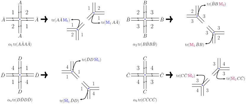
Figure 23: Splitting vertices with couplings $\mafx@alpha_{i}$

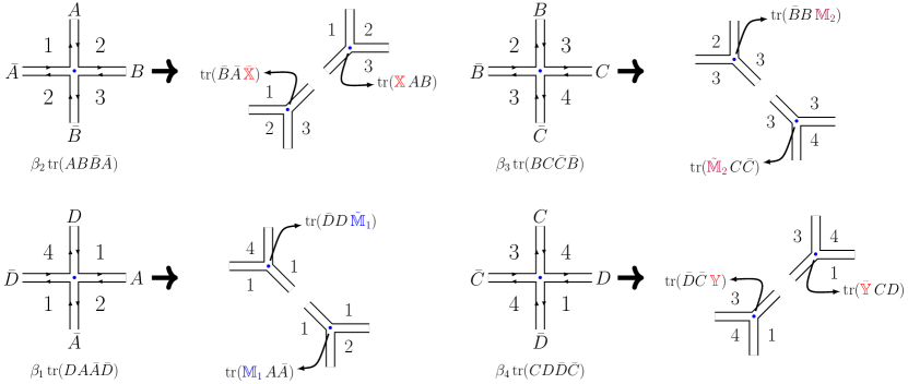
Figure 24: Splitting vertices with couplings $\mafx@beta_{i}$

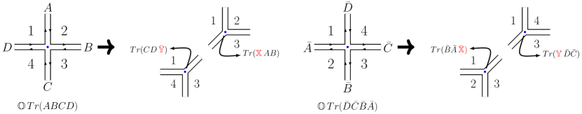
Figure 25: Splitting vertices with coupling $\mathbb{O}$ using complex matrices.

In order to reconstruct the couplings $\mafx@alpha_{i},\mafx@beta_{i}$ we impose the auxiliary matrices satisfy:

$$\langle\mathbb{M}_{1}\,\mathbb{M}_{1}\rangle=\mafx@alpha_{1} \qquad\langle\mathbb{X}\,\bar{\mathbb{X}}\rangle=\mafx@beta_{2}$$

$$\langle\mathbb{M}_{2}\,\mathbb{M}_{2}\rangle=\mafx@alpha_{2} \qquad\langle\mathbb{Y}\,\bar{\mathbb{Y}}\rangle=\mafx@beta_{4}$$

$$\langle\tilde{\mathbb{M}}_{2}\,\tilde{\mathbb{M}}_{2}\rangle=\mafx@alpha_{3} \qquad\langle\mathbb{M}_{2}\,\tilde{\mathbb{M}}_{2}\rangle=\mafx@beta_{3}$$

$$\langle\tilde{\mathbb{M}}_{1}\,\tilde{\mathbb{M}}_{1}\rangle=\mafx@alpha_{4} \qquad\langle\mathbb{M}_{1}\,\tilde{\mathbb{M}}_{1}\rangle=\mafx@beta_{1}$$ (C.16)

and similary for the non-BPS coupling:

$$\langle\mathbb{X}\,\bar{\mathbb{Y}}\rangle\,=\,\langle\bar{\mathbb{X}}\,\mathbb{Y}\rangle\,=\,\mathbb{O}$$ (C.17)

We can now arrange the three-valent vertices around reference faces $2$ and $4$ as shown in Figure 26. After removing these faces we obtain effective vertices of the form:

$$T_{\{L,\{m_{i}\},\{n_{i}\}\}}\,=\,\operatorname{tr}\left(\prod_{i=1}^{L}\left(\mathbb{M}_{1}^{m_{i}}\,\mathbb{X}\,\mathbb{M}_{2}^{n_{i}}\bar{\mathbb{X}}\right)\right)\quad\text{and}\quad\tilde{T}_{\{\tilde{L},\{\tilde{m}_{i}\},\{\tilde{n}_{i}\}\}}\,=\,\operatorname{tr}\left(\prod_{i=1}^{\tilde{L}}\left(\tilde{\mathbb{M}}_{1}^{\tilde{m}_{i}}\,\mathbb{Y}\,\tilde{\mathbb{M}}_{2}^{\tilde{n}_{i}}\bar{\mathbb{Y}}\right)\right)$$ (C.18)

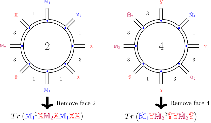
Figure 26: Integrating-out faces $2$ and $4$ gives two effective vertices, which under Wick contractions should encapsulate two faces: $1$ and $3$.

The counting of quadrangulations now follows from computing the two-point functions of these effective vertices with Wick contractions dictated by (C.4) and (C.17) and extracting the two-face coefficient $\langle T\,\tilde{T}\rangle_{2\text{ faces}}$. For instance, at genus two we have a contribution from:

$$\langle\operatorname{tr}\big{(}\mathbb{M}_{1}^{2}\,\mathbb{X}\,\mathbb{M}_{2}\,\bar{\mathbb{X}}\,\mathbb{M}_{1}\mathbb{X}\,\bar{\mathbb{X}}\big{)}\, \operatorname{tr}\big{(}\tilde{\mathbb{M}}_{1}\,\mathbb{Y}\,\tilde{\mathbb{M}}_{2}^{2}\,\bar{\mathbb{Y}}\,\mathbb{Y}\,\tilde{\mathbb{M}}_{2}\,\bar{\mathbb{Y}}\,\big{)}\rangle_{2\text{ faces}}=$$

$$4\,\mathbb{O}^{4}\mafx@alpha_{1}\mafx@alpha_{2}\mafx@alpha_{3}\mafx@beta_{1}\,+\,16\,\mathbb{O}^{4}\mafx@alpha_{1}\mafx@beta_{1}\mafx@beta_{3}^{2}\,+\,16\,\mathbb{O}^{2}\mafx@alpha_{1}\mafx@alpha_{2}\mafx@alpha_{3}\mafx@beta_{1}\mafx@beta_{2}\mafx@beta_{4}$$

$$+55\,\mathbb{O}^{2}\mafx@alpha_{1}\mafx@beta_{1}\mafx@beta_{2}\mafx@beta_{3}^{2}\mafx@beta_{4}+4\,\mafx@alpha_{1}\mafx@alpha_{2}\mafx@alpha_{3}\mafx@beta_{1}\mafx@beta_{2}^{2}\mafx@beta_{4}^{2}+12\mafx@alpha_{1}\mafx@beta_{1}\mafx@beta_{2}^{2}\mafx@beta_{3}^{2}\mafx@beta_{4}^{2}\,.$$ (C.19)

In order to compute the two-face partition function, we must consider all possible effective vertices and their corresponding symmetry factors:

$$\mathbf{Z}(\mathbb{O},\mafx@alpha_{i},\mafx@beta_{i})=\sum_{g=0}^{\infty}\,\sum_{\{\mathcal{N},\tilde{\mathcal{N}}\}\in\mathcal{M}_{g}}\,\frac{1}{s_{\mathcal{N}}s_{\tilde{\mathcal{N}}}}\,\langle T_{\mathcal{N}}\,\tilde{T}_{\tilde{\mathcal{N}}}\rangle_{2\text{-faces}}\,,$$ (C.20)

where we group the collections of indices as

$$\mathcal{N}\equiv\{L,\{m_{i}\},\{n_{i}\}\}\quad\tilde{\mathcal{N}}\equiv\{\tilde{L},\{\tilde{m}_{i}\},\{\tilde{n}_{i}\}\}\,.$$ (C.21)

Allowing for different orderings of $\{m_{i}\}$ and $\{n_{i}\}$ ($\{1,2\}\neq\{2,1\}$) in the inner sum of (C.20), then the symmetry factors are simply giving by:

$$s_{\mathcal{N}}\,=\,L\qquad\text{and}\qquad s_{\tilde{\mathcal{N}}}\,=\,\tilde{L}\,.$$ (C.22)

Furthermore the inner sum is restricted to run over the group $\mathcal{M}_{g}$, whose elements are all $\{\mathcal{N},\tilde{\mathcal{N}}\}$ that satisfy:

$$2(L+\tilde{L})\,+\,\sum_{i=1}^{L}(n_{i}+m_{i}+\tilde{n}_{i}+\tilde{m}_{i})\,=\,4g+4\,,$$ (C.23)

such that for each genus $g$ the number of fields is $4g+4$, leading two $2g+2$ squares after Wick contractions. Furthermore, from (C.4) it follows that only when $\sum_{i}m_{i}+\tilde{m}_{i}$ and $\sum_{i}n_{i}+\tilde{n}_{i}$ are even numbers are the two-point correlators non-vanishing.

The expression (C.20) admits a resummation that leads to the compact formula:

$$\mathbf{Z}(\mathbb{O},\mafx@alpha_{i},\mafx@beta_{i})\,=\,\left\langle\operatorname{tr}\log\left(\mathbb{I}-\frac{1}{\mathbb{I}-\mathbb{M}_{2}}\bar{\mathbb{X}}\frac{1}{\mathbb{I}-\mathbb{M}_{1}}\mathbb{X}\right)\operatorname{tr}\log\left(\mathbb{I}-\frac{1}{\mathbb{I}-\tilde{\mathbb{M}}_{2}}\bar{\mathbb{Y}}\frac{1}{\mathbb{I}-\tilde{\mathbb{M}}_{1}}\mathbb{Y}\right)\right\rangle_{\!2\text{ faces}}$$ (C.24)

This is the analog of (3.2), but now with couplings $\mafx@alpha_{i}$ and $\mafx@beta_{i}$ for the BPS squares. Notice that the expansion of the $\log$s in (C.24) leads to terms which do not satisfy the restriction (C.23). However, these unwanted terms do not have a two-face contribution, $\langle\text{unwanted}\rangle_{\!2\text{ faces}}=0$. So effectively, (C.20) and (C.24) are identical.

The partition function $\mathbf{A}$ that makes direct contact with the cyclic correlator studied in this paper is now given by:

$$\mathbf{A}(\mathbb{O},\mafx@alpha_{i},\mafx@beta_{i})=\sum_{g=0}^{\infty}\,\sum_{\{\mathcal{N},\tilde{\mathcal{N}}\}\in\mathcal{M}_{g}}\,\frac{1}{s_{\mathcal{N}}s_{\tilde{\mathcal{N}}}}\,\frac{1}{w_{\mathcal{N}}w_{\tilde{\mathcal{N}}}}\,\langle T_{\mathcal{N}}\,\tilde{T}_{\tilde{\mathcal{N}}}\rangle_{2\text{-faces}}$$ (C.26)

with weights:

$$w_{\mathcal{N}}\,\equiv\,w_{\{L,\{m_{i}\},\{n_{i}\}\}}\,=\,\Bigl{(}-1+\sum_{i=1}^{L}(m_{i}+1)\Bigr{)}!\Bigl{(}-1+\,\sum_{i=1}^{L}(n_{i}+1)\Bigr{)}!\,,$$ (C.27)

for which we have not found a compact re-summed formula as (C.24).

Perturbative genus computation

The two-face formulations (C.20) and (C.26) allows us to efficiently compute the partitions $\mathbf{Z}$ or $\mathbf{A}$ up to genus 4. Then under the replacement (C.7) we obtain the perturbative result in (4.5).

In the BPS limit $\mathbb{O}\to 0$, we carry on up to genus 6 by integrating out the complex matrices, and then evaluating one-face correlators of Hermitian matrices as explained in Section 3. This larger amount of data, and the inspiration we get from the extremal correlator in Appendix D.1 allows us to guess the re-summed series as:

$$\mathbf{A}(\mathbb{O}=0,\mafx@alpha_{i},\mafx@beta_{i})=\prod_{i=1}^{4}\mafx@beta_{i}\frac{\sinh\frac{1}{2}\left(\mafx@beta_{i}+\mafx@alpha_{i}+\mafx@beta_{i+1}\right)}{\frac{1}{2}\left(\mafx@beta_{i}+\mafx@alpha_{i}+\mafx@beta_{i+1}\right)}\,.$$ (C.28)

Under the replacement (C.7), we obtain the result in (3.10).

In fact we further found that formula (C.28) can be extended to find the BPS part of a larger class of cyclic correlators, as we present in Appendix D.2.

Appendix D Other Results On Quadrangulations

D.1 $(n+1)$-Point Extremal Correlators in DSL

In this appendix, we review the computation of protected extremal correlators of the form

$$E_{n}=\langle\operatorname{tr}(Z^{J_{1}})\operatorname{tr}(Z^{J_{2}})\cdots\operatorname{tr}(Z^{J_{n}})\operatorname{tr}(\bar{Z}^{J_{R}})\rangle$$ (D.1)

with $J_{R}=J_{1}+\cdots+J_{n}$, in the double scaling limit $J_{i}\to\infty$, $N_{\text{c}}\to\infty$ and $J_{i}/\sqrt{N_{\text{c}}}$ fixed. In fact the result is known at finite $N_{\text{c}}$ and $J_{i}$ from [4, 6]. In the DSL it is given by:

$$E_{n}(J_{i},N_{\text{c}})\,\overset{\text{DSL}}{=}\,J_{R}^{-2}(2N_{\text{c}})^{n}\,\prod_{i=1}^{n}\sinh\left(\frac{J_{i}J_{R}}{2N_{\text{c}}}\right)\,.$$ (D.2)

Here, we would like to present how to reproduce this result by counting quadrangulations and using integrating-in and -out graph operations.

In the DSL, the correlator $E_{n}$ can be reconstructed in a similar fashion as the cyclic correlator of this article. The skeleton graphs that dominate are also given by quadrangulations, and to obtain $E_{n}$ we must count them and dress them with the lengths $J_{i}$ by performing a Borel-type transformation.

All squares involved include the reservoir $R$ twice, and the corresponding dual four-valent vertices are given in the matrix action:

$$S^{(\text{E})}_{n}=-\sum_{a=1}^{n}\operatorname{tr}(A_{a}\bar{A}_{a})\,+\,\frac{1}{2}\sum_{a=1}^{n}\sum_{b=1}^{n}\,\mafx@alpha_{a,b}\,\operatorname{tr}(A_{a}A_{b}\bar{A}_{b}\bar{A}_{a})$$ (D.3)

with couplings $\mafx@alpha_{a,b}=\mafx@alpha_{b,a}$ associated to squares of the form [RaRb].

The relevant Borel-transformed partition function (the analog of (C.5)) coming from the matrix model (D.3) is

$$\mathbf{A}^{(\text{E})}_{n}(\mafx@alpha_{a,b})=\sum_{g=0}^{\infty}\,\sum_{T_{g}=\{t_{1},\cdots t_{n+2g-1}\}\in V^{(\text{E})}_{4}}\frac{1}{\text{\text{sym}($T_{g}$)}}\frac{1}{\text{\text{weight}($T_{g}$)}}\left\langle\prod_{m=1}^{n+2g-1}\,t_{m}\right\rangle_{(n+1)\text{ faces}}\,,$$ (D.4)

where now $T_{g}$ is a subset of $(n+2g-1)$ four-valence vertices with couplings chosen from $V^{(\text{E})}_{4}=\{\mafx@alpha_{a,b}\operatorname{tr}(A_{a}A_{b}\bar{A}_{b}\bar{A}_{a})\}_{a,b=1,\cdots,n}$ with at least one occurrence of $A_{a}$ for $a=1,\cdots,n$.

The symmetry factor $\text{sym}(T_{g})$ has a factor of 2 for each vertex of the form $\operatorname{tr}(A_{a}A_{a}\bar{A}_{a}\bar{A}_{a})$, and a $k!$ when $T_{g}$ contains a vertex repeated $k$ times. The weight factor is given by:

$$\text{weight}(T_{g})\,=\,\prod_{i=1}^{n}(m_{A_{i}}-1)!$$ (D.5)

where $m_{A_{i}}$ counts the number of occurrences of $A_{i}$ in the subset $T_{g}$.

This partition function $\mathbf{A}$ can be identified with the DSL of the extremal correlator under the replacement:

$$E_{n}(J_{i},N_{\text{c}})\,\overset{\mathrm{DSL}}{=}N_{\text{c}}^{n-1}\,\mathbf{A}^{(\text{E})}_{n}(\mafx@alpha_{a,b})\big{|}_{\mafx@alpha_{a,b}\to{J_{a}J_{b}}/{N_{\text{c}}}}$$ (D.6)

We can simplify the correlators $\langle\cdots\rangle_{(n+1)\text{ faces}}$ in (D.4) by performing integrating-in and -out operations. First, we integrate-in to obtain three-valent vertices where the faces lying between their edges are $(RRa)$ as shown in figure Figure 27.

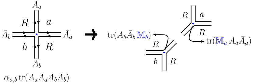
Figure 27: Splitting a BPS vertex by introducing hermitian matrices $\mathbb{M}_{a}$ and $\mathbb{M}_{b}$, which satisfy $\langle\mathbb{M}_{a}\mathbb{M}_{b}\rangle=\mafx@alpha_{a,b}$.

Then, we can arrange all vertices of the form $(RRa)$ around the face $a$, for all $a=1,\cdots,n$, as shown in Figure 28.

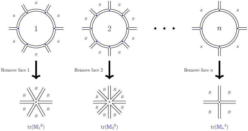
Figure 28: Integrating-out all faces except the reservoir $R$.

Finally, by removing these $n$ reference faces, we obtain $n$ effective vertices, with the only remaining face being the reservoir $R$. So the partition $\mathbf{A}^{(E)}_{n}$ is now effectively computed by a sum of one-face correlators:

$$\mathbf{A}^{(\text{E})}_{n}(\mafx@alpha_{a,b})=\sum_{g=0}^{\infty}\,\sum_{i_{1}+\cdots+i_{n}=2(n+2g-1)}\frac{\langle\operatorname{tr}(\mathbb{M}_{1}^{i_{1}})\cdots\operatorname{tr}(\mathbb{M}_{n}^{i_{n}})\rangle_{1\text{ face}}}{i_{1}!\cdots i_{n}!}\,=\,\left\langle\prod_{a=1}^{n}\operatorname{tr}\left(e^{\mathbb{M}_{a}}-\mathbb{I}\right)\right\rangle_{1\text{ face}}\,$$ (D.7)

where all indices $i_{m}>0$, and the couplings appear in the Wick contractions as:

$$\langle\mathbb{M}_{a}\mathbb{M}_{b}\rangle\,=\,\mafx@alpha_{a,b}\,.$$ (D.8)

We have computed this partition function (D.7) for the first few genera, and found a match against (D.2) under the replacement (D.6). We have further recognized that in terms of couplings $\mafx@alpha_{a,b}$, the partition function evaluates to:

$$\mathbf{A}^{(\text{E})}_{n}(\mafx@alpha_{a,b})=\left\langle\prod_{a=1}^{n}\operatorname{tr}\left(e^{\mathbb{M}_{a}}-\mathbb{I}\right)\right\rangle_{1\text{ face}}\,=\,P_{n}(\mafx@alpha_{a,b})\prod_{a=1}^{n}\frac{\sinh\left(\frac{1}{2}\sum_{b=1}^{n}\mafx@alpha_{a,b}\right)}{\frac{1}{2}\sum_{b=1}^{n}\mafx@alpha_{a,b}}\,.$$ (D.9)

The prefactor $P_{n}$ is a non-factorizable homogeneous polynomial of degree $n-1$ in the couplings $\mafx@alpha_{a,b}$, with $a\neq b$, and is independent of the genus. For $n=3$ and $n=4$, it is simply given by:

$$P_{n=3} =\mafx@alpha_{1,2}\,\mafx@alpha_{1,3}+\,\mafx@alpha_{1,2}\,\mafx@alpha_{2,3}+\,\mafx@alpha_{1,3}\,\mafx@alpha_{2,3}\,,$$ (D.10)

$$P_{n=4} =\mafx@alpha_{1,2}\mafx@alpha_{3,4}(\mafx@alpha_{1,3}+\mafx@alpha_{1,4}+\mafx@alpha_{2,3}+\mafx@alpha_{2,4})+\mafx@alpha_{1,3}\mafx@alpha_{2,4}(\mafx@alpha_{1,2}+\mafx@alpha_{1,4}+\mafx@alpha_{2,3}+\mafx@alpha_{3,4})$$

$$\quad+\mafx@alpha_{1,4}\mafx@alpha_{2,3}(\mafx@alpha_{1,2}+\mafx@alpha_{1,3}+\mafx@alpha_{2,3}+\mafx@alpha_{2,4})+\mafx@alpha_{1,2}\mafx@alpha_{1,3}\mafx@alpha_{1,4}+\mafx@alpha_{1,2}\mafx@alpha_{2,3}\mafx@alpha_{2,4}$$

$$\quad+\mafx@alpha_{1,3}\mafx@alpha_{2,3}\mafx@alpha_{3,4}+\mafx@alpha_{1,4}\mafx@alpha_{2,4}\mafx@alpha_{3,4}\,.$$ (D.11)

We have not found its closed form for generic $n$, although we know it explicitly up to $n=6$. It is related to the planar contribution of the DSL of the extremal correlator:

$$\lim_{N_{\text{c}}\to\infty}E_{n}\overset{\mathrm{DSL}}{=}P_{n}(\mafx@alpha_{a,b})\big{|}_{\mafx@alpha_{a,b}\to J_{a}J_{b}}=(J_{1}+\cdots+J_{n})^{n-2}\,\,\prod_{i=1}^{n}J_{i}\,=\,J_{R}^{n-2}\,\prod_{i=1}^{n}J_{i}\,.$$ (D.12)

D.2 $n$-Point Cyclic Correlators In DSL

Finally, we consider the $n$-point cyclic correlator shown in Figure 29. For $\mathcal{N}=4$ SYM, only the correlators with $n\leq 6$ are realizable, while for higher $n$ the theory does not admit enough R-charge polarizations to prevent other connections that break the cyclic pattern. Furthermore, as explained in Section 4, see paragraph before (4.6), for $n>4$ only BPS quadrangulations dominate.

The relevant matrix model to count these quadrangulations has the action

$$S^{(\text{C})}_{n}=-\sum_{i=1}^{n}\operatorname{tr}(A_{i}\bar{A}_{i})\,+\,\sum_{i=1}^{n}\frac{\mafx@alpha_{i}}{2}\operatorname{tr}(A_{i}\,\bar{A}_{i}A_{i}\,\bar{A}_{i})+\mafx@beta_{i}\,\operatorname{tr}(A_{i}\bar{A}_{i}\bar{A}_{i-1}A_{i-1})$$ (D.13)

Based on direct computations of the relevant correlators of four-valent vertices up to genus two, we predict the generalization of (C.28) is:

$$\mathbf{A}^{(\text{C})}_{n}(\mafx@alpha_{i},\mafx@beta_{i})=\prod_{a=1}^{n}\mafx@beta_{i}\frac{\sinh\left(\frac{1}{2}\left(\mafx@beta_{i}+\mafx@alpha_{i}+\mafx@beta_{i+1}\right)\right)}{\frac{1}{2}\left(\mafx@beta_{i}+\mafx@alpha_{i}+\mafx@beta_{i+1}\right)}\,,$$ (D.14)

where $\mathbf{A}^{(\text{C})}_{n}$ is defined analogously to (C.5), with the four-valent vertices in (D.13), and demanding now $n$ faces $(\langle\cdots\rangle_{n\text{ faces}})$. The corresponding cyclic correlator in the DSL is obtained by introducing the bridge lengths $k_{i}$ with the replacement $\mafx@alpha_{i}\to{k_{i}^{2}}/{N_{\text{c}}^{2}}$ and $\mafx@beta_{i}\to{k_{i-1}k_{i}}/{N_{\text{c}}}$ with $k_{0}\equiv k_{n}$.

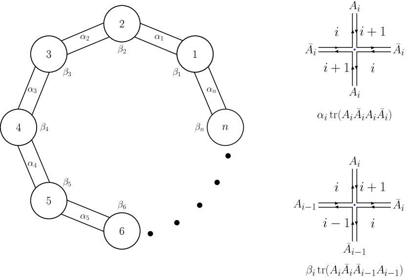
Figure 29: Cyclic correlator and four-valent vertices dual to the BPS squares $[i(i+1)i(i+1)]$ and $[i(i+1)i(i-1)]$.

References

- [1] F. Coronado, “Perturbative Four-Point Functions in Planar 4 SYM from Hexagonalization”, JHEP 1901, 056 (2019), arxiv:1811.00467.
- [2] F. Coronado, “Bootstrapping the simplest correlator in planar 4 SYM at all loops”, arxiv:1811.03282.
- [3] I. Kostov, V. B. Petkova and D. Serban, “Determinant formula for the octagon form factor in 4 SYM”, arxiv:1903.05038.
- [4] C. Kristjansen, J. Plefka, G. W. Semenoff and M. Staudacher, “A new double-scaling limit of 4 super Yang–Mills theory and PP-wave strings”, Nucl. Phys. B643, 3 (2002), hep-th/0205033.
- [5] N. R. Constable, D. Z. Freedman, M. Headrick, S. Minwalla, L. Motl, A. Postnikov and W. Skiba, “PP-wave string interactions from perturbative Yang–Mills theory”, JHEP 0207, 017 (2002), hep-th/0205089.
- [6] N. Beisert, C. Kristjansen, J. Plefka, G. W. Semenoff and M. Staudacher, “BMN Correlators and Operator Mixing in 4 Super Yang–Mills Theory”, Nucl. Phys. B650, 125 (2003), hep-th/0208178.
- [7] N. R. Constable, D. Z. Freedman, M. Headrick and S. Minwalla, “Operator mixing and the BMN correspondence”, JHEP 0210, 068 (2002), hep-th/0209002.
- [8] N. Beisert, C. Kristjansen, J. Plefka and M. Staudacher, “BMN Gauge Theory as a Quantum Mechanical System”, Phys. Lett. B558, 229 (2003), hep-th/0212269.
- [9] D. Berenstein, J. M. Maldacena and H. Nastase, “Strings in flat space and pp waves from 4 Super Yang Mills”, JHEP 0204, 013 (2002), hep-th/0202021.
- [10] T. Fleury and S. Komatsu, “Hexagonalization of Correlation Functions”, JHEP 1701, 130 (2017), arxiv:1611.05577.
- [11] B. Eden and A. Sfondrini, “Tessellating cushions: four-point functions in 4 SYM”, JHEP 1710, 098 (2017), arxiv:1611.05436.
- [12] B. Eden, Y. Jiang, D. le Plat and A. Sfondrini, “Colour-dressed hexagon tessellations for correlation functions and non-planar corrections”, JHEP 1802, 170 (2018), arxiv:1710.10212.
- [13] T. Fleury and S. Komatsu, “Hexagonalization of Correlation Functions II: Two-Particle Contributions”, JHEP 1802, 177 (2018), arxiv:1711.05327.
- [14] T. Bargheer, J. Caetano, T. Fleury, S. Komatsu and P. Vieira, “Handling Handles: Nonplanar Integrability in Supersymmetric Yang–Mills Theory”, Phys. Rev. Lett. 121, 231602 (2018), arxiv:1711.05326.
- [15] T. Bargheer, J. Caetano, T. Fleury, S. Komatsu and P. Vieira, “Handling handles. Part II. Stratification and Data Analysis”, JHEP 1811, 095 (2018), arxiv:1809.09145.
- [16] H. Dorn, N. Drukker, G. Jorjadze and C. Kalousios, “Space-like minimal surfaces in ”, JHEP 1004, 004 (2010), arxiv:0912.3829.
- [17] V. A. Kazakov, “Solvable matrix models”, hep-th/0003064.
- [18] A. Zvonkin, “Matrix integrals and map enumeration: An accessible introduction”, Mathematical and Computer Modelling 26, 281 (1997).
- [19] T. W. Brown, “Complex matrix model duality”, Phys. Rev. D83, 085002 (2011), arxiv:1009.0674.
- [20] P. G. de Gennes, “Exponents for the excluded volume problem as derived by the Wilson method”, Physics Letters A 38, 339 (1972).
- [21] P. G. de Gennes and T. A. Witten, “Scaling Concepts in Polymer Physics”, Physics Today 33, 51 (1980).
- [22] J. Cardy, “Scaling and Renormalization in Statistical Physics”, Cambridge Lecture Notes in Physics, Cambridge University Press (1996).
- [23] D. Sherrington and S. Kirkpatrick, “Solvable Model of a Spin-Glass”, Phys. Rev. Lett. 35, 1792 (1975).
- [24] J. R. L. de Almeida and D. J. Thouless, “Stability of the Sherrington-Kirkpatrick solution of a spin glass model”, Journal of Physics A: Mathematical and General 11, 983 (1978).
- [25] F. Morone, F. Caltagirone, E. Harrison and G. Parisi, “Replica Theory and Spin Glasses”, arxiv:1409.2722.
- [26] E. Brézin and S. Hikami, “Characteristic Polynomials of Random Matrices”, Communications in Mathematical Physics 214, 111 (2000).
- [27] E. Brézin and S. Hikami, “Vertices from replica in a random matrix theory”, J. Phys. A40, 3545 (2007), arxiv:0704.2044.
- [28] E. Brézin and S. Hikami, “Intersection theory from duality and replica”, Commun. Math. Phys. 283, 507 (2008), arxiv:0708.2210.
- [29] E. Brézin and S. Hikami, “Duality and replicas for a unitary matrix model”, JHEP 1007, 067 (2010), arxiv:1005.4730.
- [30] S. Bellucci and C. Sochichiu, “On matrix models for anomalous dimensions of super Yang–Mills theory”, Nucl. Phys. B726, 233 (2005), hep-th/0410010.
- [31] P. Di Francesco, “Rectangular matrix models and combinatorics of colored graphs”, Nucl. Phys. B648, 461 (2003), cond-mat/0208037.
- [32] S. H. Shenker, “The Strength of nonperturbative effects in string theory”, in: “The Large N expansion in quantum field theory and statistical physics: From spin systems to two-dimensional gravity”, pp. 809, ed.: E. Brézin and S. R. Wadia, World Scientific (1993).
- [33] J. Polchinski, “Combinatorics of boundaries in string theory”, Phys. Rev. D50, R6041 (1994), hep-th/9407031.
- [34] J. M. Maldacena, G. W. Moore, N. Seiberg and D. Shih, “Exact vs. semiclassical target space of the minimal string”, JHEP 0410, 020 (2004), hep-th/0408039.
- [35] R. Gopakumar, “Open-Closed-Open String Duality”, talk at the Johannesburg workshop: ‘Correlation Functions and the AdS/CFT Correspondence’ (April 27, 2010), http://neo.phys.wits.ac.za/workshop_2/pdfs/rajesh.pdf.
- [36] P. Di Francesco and C. Itzykson, “A Generating function for fatgraphs”, Ann. Inst. H. Poincare Phys. Theor. 59, 117 (1993), hep-th/9212108.
- [37] A. Mironov and A. Morozov, “On the complete perturbative solution of one-matrix models”, Phys. Lett. B771, 503 (2017), arxiv:1705.00976.
- [38] I. K. Kostov, “O() Vector Model on a Planar Random Lattice: Spectrum of Anomalous Dimensions”, Mod. Phys. Lett. A4, 217 (1989).
- [39] T. Bargheer, F. Coronado, V. Gonçalves and P. Vieira, “Octagons II: Strong Coupling”, to appear.
- [40] J. Maldacena, D. Simmons-Duffin and A. Zhiboedov, “Looking for a bulk point”, JHEP 1701, 013 (2017), arxiv:1509.03612.
- [41] R. A. Janik, P. Surowka and A. Wereszczynski, “On correlation functions of operators dual to classical spinning string states”, JHEP 1005, 030 (2010), arxiv:1002.4613.
- [42] T. Klose and T. McLoughlin, “A Light-Cone Approach to Three-Point Functions in ”, JHEP 1204, 080 (2012), arxiv:1106.0495.
- [43] J. A. Minahan, “Holographic three-point functions for short operators”, JHEP 1207, 187 (2012), arxiv:1206.3129.
- [44] T. Bargheer, J. A. Minahan and R. Pereira, “Computing Three-Point Functions for Short Operators”, JHEP 1403, 096 (2014), arxiv:1311.7461.
- [45] I. K. Kostov and M. Staudacher, “Two-dimensional chiral matrix models and string theories”, Phys. Lett. B394, 75 (1997), hep-th/9611011.
- [46] V. A. Kazakov, “Exactly solvable potts models, bond and tree like percolation on dynamical (random) planar lattice”, in: “Field Theory on the Lattice. International Symposium, Seillac, France, September 28 - October 2, 1987”, Nuclear Physics B - Proceedings Supplements, pp. 93-97.
- [47] V. A. Kazakov, M. Staudacher and T. Wynter, “Character expansion methods for matrix models of dually weighted graphs”, Commun. Math. Phys. 177, 451 (1996), hep-th/9502132.
- [48] V. A. Kazakov, M. Staudacher and T. Wynter, “Almost flat planar diagrams”, Commun. Math. Phys. 179, 235 (1996), hep-th/9506174.
- [49] V. A. Kazakov, M. Staudacher and T. Wynter, “Exact solution of discrete two-dimensional gravity”, Nucl. Phys. B471, 309 (1996), hep-th/9601069.
- [50] S. Corley, A. Jevicki and S. Ramgoolam, “Exact correlators of giant gravitons from dual 4 SYM theory”, Adv. Theor. Math. Phys. 5, 809 (2002), hep-th/0111222.
- [51] T. W. Brown, P. J. Heslop and S. Ramgoolam, “Diagonal multi-matrix correlators and BPS operators in 4 SYM”, JHEP 0802, 030 (2008), arxiv:0711.0176.
- [52] Ö. Gürdoğan and V. Kazakov, “New Integrable 4D Quantum Field Theories from Strongly Deformed Planar 4 Supersymmetric Yang–Mills Theory”, Phys. Rev. Lett. 117, 201602 (2016), arxiv:1512.06704.
- [53] J. Caetano, Ö. Gürdoğan and V. Kazakov, “Chiral limit of 4 SYM and ABJM and integrable Feynman graphs”, JHEP 1803, 077 (2018), arxiv:1612.05895.
- [54] B. Basso and L. J. Dixon, “Gluing Ladder Feynman Diagrams into Fishnets”, Phys. Rev. Lett. 119, 071601 (2017), arxiv:1705.03545.
- [55] B. Basso, J. Caetano and T. Fleury, “Hexagons and Correlators in the Fishnet Theory”, arxiv:1812.09794.
- [56] N. Berkovits, “Sketching a Proof of the Maldacena Conjecture at Small Radius”, arxiv:1903.08264.
- [57] N. Gromov and A. Sever, “The Holographic Fishchain”, arxiv:1903.10508.
- [58] V. A. Kazakov, “Field theory as a matrix model”, Nucl. Phys. B587, 645 (2000), hep-th/0003065.
- [59] A. Hatcher, “On triangulations of surfaces”, Topology and its Applications 40, 189 (1991).
- [60] J. Harer and D. Zagier, “The Euler characteristic of the moduli space of curves”, Invent. Math. 85, 457 (1986).