One of the well-studied equations in the theory of ODEs is the Mathieu differential equation. A common approach for obtaining solutions is to seek solutions via Fourier series by converting the equation into an infinite system of linear equations for the Fourier coefficients. We study the asymptotic behavior of these Fourier coefficients and discuss the ways in which to numerically approximate solutions. We present both theoretical and numerical results pertaining to the stability of the Mathieu differential equation and the properties of solutions. Further, based on the idea of using Fourier series, we provide a method in which the Mathieu differential equation can be generalized to be defined on the infinite Sierpinski gasket. We discuss the stability of solutions to this fractal differential equation and describe further results concerning properties and behavior of these solutions.
1. Introduction
The Mathieu differential equation, as will be defined in Section 2, takes the form , where are fixed, and . Named after French mathematician Émile Léonard Mathieu (1835-1890), the origin of the Mathieu differential equation stems from real-world phenomena. For example, it describes the motion of a pendulum subject to a periodic driving force. See [21] for more details.
One topic pertaining to the Mathieu differential equation which has been much researched is the stability of solutions. See [2, 10, 16, 17, 28]. Readers may also read [21, 18] for a brief introduction to this area. Most of the existing literature concerns the parameter space, i.e. the space of - pairs, whose choices can drastically alter the behavior of solutions. This paper presents research results and new phenomena both on the parameter space and on solutions.
On the other hand, another area of mathematics which has been actively researched in recent years is analysis on fractals, based on J. Kigami’s construction of Laplacians on post-critically finite self-similar sets. See [13, 15, 14, 22]. It is of interest to define and study the Mathieu differential equation on fractal domains, and one suitable domain is the infinite Sierpinski gasket developed by R.S. Strichartz [24]. Existing research on the infinite Sierpinski gasket and on other ‘fractafolds’ be found in [12, 20, 23, 25, 26, 27]. In particular, we will use the important result concerning the spectrum of the Laplacian on the infinite Sierpinski gasket by A. Teplyaev [27]. We will explore a way to generalize the Mathieu differential equation to be defined on the infinite Sierpinski gasket.
This paper is organized as follows. In Section 2, we provide relevant background on the Mathieu differential equation, give definitions which will be used throughout the remainder of the paper, and describe some of the methods used to study the relationship that the values of and have to the solutions of the equation; in doing so we will discuss ‘transition curves’ and the ‘truncation method’ used to study solutions to the Mathieu differential equation. In Section 3 we present a number of proofs for theorems pertinent to the Mathieu differential equation and provide justification for the methods presented in Section 2. Some of our methods and proofs are modified versions from [1, 9]. In Section 4 we provide a discussion of computational results in studying the Mathieu differential equation, including results related to the asymptotic behavior of transition curves and the convergence of solutions. In Section 5 we give an overview of the Sierpinski gasket () and provide definitions of various terms in fractal analysis, such as the fractal Laplacian and the infinite Sierpinski gasket (), to be used in the remaining sections. In Section 6 we extend the content of Sections 2, 3, and 4 to the fractal setting by explaining how the ‘Mathieu differential equation defined on the real line’ can be generalized to a ‘Mathieu differential equation defined on the infinite Sierpinski gasket.’ We describe how solutions to this generalization can be studied by considering solutions expanded as a linear combination of eigenfunctions of the fractal Laplacian. We also describe how the ‘truncation method’ on the line can be used to study the Mathieu differential equation on . In Section 7 we provide computational results and observations about the shape and asymptotic behavior of the transition curves for the Mathieu differential equation on and also about the behavior of solutions. In Section 8 we describe further research that can be done on the Mathieu differential equation and its fractal generalizations. Section 9, the Appendix, describes an alternate approach to the ‘truncation method’ which involves partitioning Fourier coefficients into various equivalence classes.
A website for this research has been created at http://pi.math.cornell.edu/~aac254/. We invite the reader to visit this website, as it contains plots, graphs, data, and other information gathered from the research.
2. Definitions and Methods
In this section we give formal definitions pertaining to the Mathieu differential equation on the real line and then describe the main methods used to study it.
2.1. Fourier Expansion and Matrix Form
Let us suppose we have a periodic solution with period or to the Mathieu differential equation. In this case, we can write the Fourier series expansion of as
If we plug this Fourier series for into the MDE, rearrange terms, and use some trigonometric identities, we find that the function given above solves the MDE if and only if the two infinite systems of linear homogeneous equations shown below for the cosine and sine coefficients are satisfied. See [18] and [21] for more details.
and
To solve these systems of equations, we consider putting them into matrix form. Readers can check that the above two systems of equations are equivalent to the following four equations in matrix form collectively, which correspond to cosine or sine coefficients with even or odd indexes. All the matrices are tridiagonal. For the cosine coefficients with even indexes, we have
For the sine coefficients with even indexes, we have
For cosine coefficients with odd indexes, we have
For sine coefficients with odd indexes, we have
We can solve the above four matrix equations separately. If either of the first two equations has a nontrivial solution in , then the MDE has a -periodic solution, since
solves the MDE and is -periodic, comparing with Remark 2.4. Similarly, if either the third or fourth equations has a nontrivial solution in , then the MDE has a -periodic solution, since
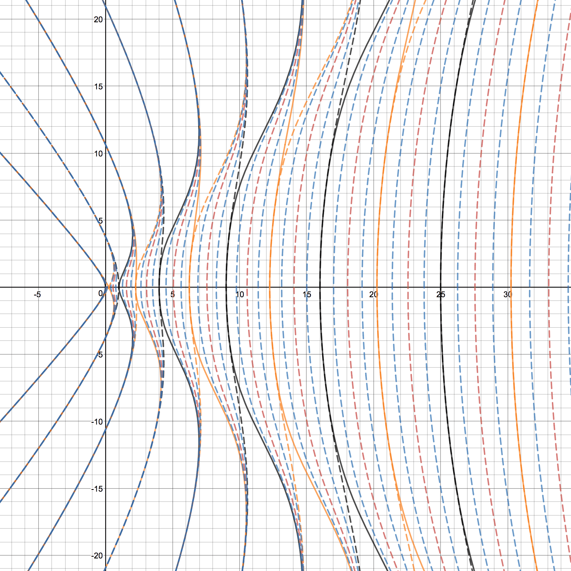
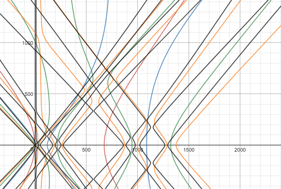
solves the MDE and is -periodic, also comparing with Remark 2.4. Interested readers can also read the appendix for equations in matrix form for periodic solutions with larger periods, say with an arbitrary positive integer. Now we return our discussion to Figure LABEL:deltaepsilonplanefigure, where we plot the stable and unstable regions. According to Theorem LABEL:transitioncurvetheorem, the transition curves consist of pairs with nontrivial - or -periodic solutions. Equivalently, by the above discussion, lies on a transition curve if and only if at least one of the four equations in matrix form discussed above has a nontrivial solution in . Since we develop four different equations in matrix form, we use different colors (orange and black) and line formats (solid and dashed) in Figure LABEL:deltaepsilonplanefigure to distinguish between the four matrix equations:
-
•
If falls on a black solid line, then the equation has a nontrivial solution.
-
•
If falls on a black dashed line, then the equation has a nontrivial solution.
-
•
If falls on an orange solid line, then the equation has a nontrivial solution.
-
•
If falls on an orange dashed line, then the equation has a nontrivial solution.
2.2. Truncation Method
In finite-dimensional linear algebra, a homogeneous matrix system of equations , where is an matrix, has a nontrivial solution if and only if the determinant of is zero. Although our four systems of matrix equations above are infinite, we hope to use techniques from finite-dimensional linear algebra to study the properties of these infinite systems. For each infinite matrix, fix and consider its leading principal submatrix. Below we give the truncated matrices and of and respectively, as examples. and are defined similarly.
Taking the determinant of each truncated matrix yields an algebraic expression involving and . Setting each expression equal to zero, we can then plot each equation in the - plane and obtain a set of algebraic curves in the variables and . If we choose sufficiently large, the - curves derived from the truncated matrices will be very close to the true transition curves corresponding to the infinite matrices. This statement is made precise by Ikebe et al. in [1], and we present their results in Section 3.2.
3. Three-Term Recurrence Relations and Truncations of the Infinite Matrices
In this section, we will provide theoretical foundation for the methods we use. In doing so we will discuss the asymptotic convergence of Fourier coefficients and provide an error estimate for the truncation method we use for approximating the transition curves. (We will extend these techniques to the fractal MDE in later sections.) In this section, we work in generality by considering matrices of the form
| (3.1) |
where for , and ; further, we assume that and are bounded sequences and that . Note that matrices and as defined in Section 2.2 are special cases of (3.1). In addition, we always assume , for all , in this section. We will consider equations of the form
| (3.2) |
where is a real sequence.
3.1. Asymptotic Behavior of
Three-term recurrence relations (TTRRs) and difference equations have been well-studied throughout the last century. Since (3.2) naturally gives a TTRR,
| (3.3) |
we can use existing theorems to study the asymptotic behavior of the sequence as . Below we first present the well-known Poincaré Theorem (see [9]), also called the Poincaré-Perron Theorem, which describes the asymptotic behavior of solutions to general TTRRs, and then we will see how the theorem applies to the equations above.
Theorem 3.1 (Poincaré-Perron Theorem, [9]).
For , let with and . Let and denote the zeros of the characteristic equation . Then, if , the difference equation has two linearly independent solutions and satisfying
If , then
for any nontrivial solution to the recurrence relation. ∎
With this theorem in mind, we consider the TTRR
| (3.4) |
where and neither of which contains as one of its terms, are uniformly bounded, and where as . Notice that, with our assumptions, the solution of Equation 3.4 is uniquely determined by specifying the first two terms and . We can derive the following proposition from the Poincaré-Perron Theorem, adapting its proof directly from the proof of the Poincaré-Perron Theorem in [9].
Proposition 3.2.
Assume and , neither of which is equal to the zero sequence, are uniformly bounded, and assume that as . Then the TTRR (3.4) has two linearly independent solutions and satisfying
Proof. The proof is modified directly from the proof for the Poincaré-Perron Theorem in [9]. For convenience, we assume for any , since otherwise we can consider the TTRR defined for for some large . Let . Then the TTRR becomes
By the Poincaré-Perron theorem, there exists a pair of linearly independent solutions of this new recurrence, and , satisfying
For sufficiently large, does not vanish. Indeed, if for some then the TTRR implies , which cannot happen if were sufficiently large (since ). Similarly, for sufficiently large does not vanish, for if for some then , which cannot happen for sufficiently large (since ). Let and . Then
Multiplying each side by , we get
Subtracting one equation from the other, we obtain
So, since
we have
Therefore,
and
Let be an arbitrary solution to the TTRR 3.4. We say is a minimal solution of the TTRR if it obeys , and we say is a dominant solution of the TTRR if it satisfies . Note that if is a minimal solution and if is a dominant solution. We can apply Proposition 3.2 to study Equation 3.3, since Equation 3.3 consists of an equation for and a TTRR of the form 3.4.
Corollary 3.3.
Assume . (a). Equation 3.2 has a unique solution up to multiplication by a constant. (b). Let be a nontrivial solution to Equation (3.2). If , then will decay with the asymptotic behavior . If , then will diverge with the asymptotic behavior .
Proof. It is equivalent to studying Equation 3.3.
(a). Given , we can solve inductively, which gives us a solution to Equation 3.3. In this way, any solution to Equation 3.3 is uniquely determined by .
(b) Any solution can be written as a linear combination of and as given in in Proposition 3.2, and hence there exist such that for all . Note that if then is a dominant solution, and if then is a minimal solution.
If then and thus cannot be a dominant solution; thus, we must have and hence . On the other hand, if then and hence .
Corollary 3.3 shows that there is a sharp contrast between the two possible types of behavior that a solution to Equation (3.2) can have. Since and are bounded sequences, when are fixed and properly chosen any solution to (3.2) will converge to very rapidly; otherwise, all nontrivial solutions will tend to infinity very fast.
If is an initial value which corresponds to a minimal solution, Proposition 3.2 shows that numerically computing the solution with the forward recursion method is unstable, since a small error in computation will lead to a dominant solution, in which explodes. On the other hand, the backward recursion method can give a good approximation for a minimal solution. In [9], detailed discussions are given on this method, as well as a corresponding error estimate. We briefly state the result here.
3.2. The Truncation Method
In this part, we introduce the truncation method for determining which pairs yield nontrivial solutions of (3.2). We start from the observation
where is the identity matrix and the shorthand notation is used in the last equality. Clearly, for a fixed , equation (3.2) has nontrivial solutions if and only if is an eigenvalue of . The eigenvalue problem for infinite tridiagonal matrices has been widely studied. In [1], there is a result on the error between eigenvalues of the truncated matrices and those of the corresponding infinite matrix. We state the result in Theorem 3.5 below. Here we consider the infinite symmetric tridiagonal matrix of the form
where as and bounded. Denote its truncation by , i.e.,
Theorem 3.5.
([1]) Let and be given as above.
(a). has pure point spectrum.
(b). If is a given simple eigenvalue of , then there exists, for each , an eigenvalue of such that the sequence satisfies as . For any such sequence the error is given by
where is an eigenvector corresponding to . ∎
We can extend the above result to nonsymmetric tridiagonal matrices.
Theorem 3.6.
Let be an infinite tridiagonal matrix of the form
where as , and and are bounded, positive, and nonzero. Let be the truncation of . If is a given simple eigenvalue of , then there exists, for each , an eigenvalue of such that the sequence satisfies as . For any such sequence the error is given by
where and where is an eigenvector corresponding to . ∎
Proof. (a) Let
We observe that
It is clear that is a self-adjoint operator from to with pure point spectrum by Theorem 3.5. Let
where . Clearly, the eigenvalue equation holds if and only if in a pointwise sense, where is the identity transformation. In addition, from Corollary 3.3 we deduce that there is a one-to-one correspondence between eigenvectors of and in . Indeed, if is an eigenvector of in , we have because by Corollary 3.3, which implies is an eigenvector of in , and for the same reason if is an eigenvector of then is an eigenvector of in . Now, using Theorem 3.5 we deduce that there is a sequence of eigenvalues of the truncated that converges to the eigenvalue of and hence of , since and have the same eigenvalues. In addition, noticing that, for each , has the same eigenvalue as , we see that there is a sequence of eigenvalues of which converges to . Lastly, the error estimate comes by applying Theorem 3.5 to with the eigenvector .
4. Observations and Analysis for the Mathieu Differential Equation on the Line
The Mathieu differential equation has been an important topic in differential equations due to its numerous real-world applications. However, most of the existing work on the MDE focuses on theoretical analysis of the stable and unstable regions of the - plane, such as the asymptotic behavior of the transition curves, and there has not been much computational work done on the stability curves as well as on the solutions to the Mathieu differential equation. In this section, in addition to describing some of our theoretical results, we will explain our computational results on the intricate shape of the - curves and on the converging behavior of the solutions.
4.1. The - Plot
In this part, we use the truncation method introduced in Section 2 and Section 3 to study the - curves in more detail.
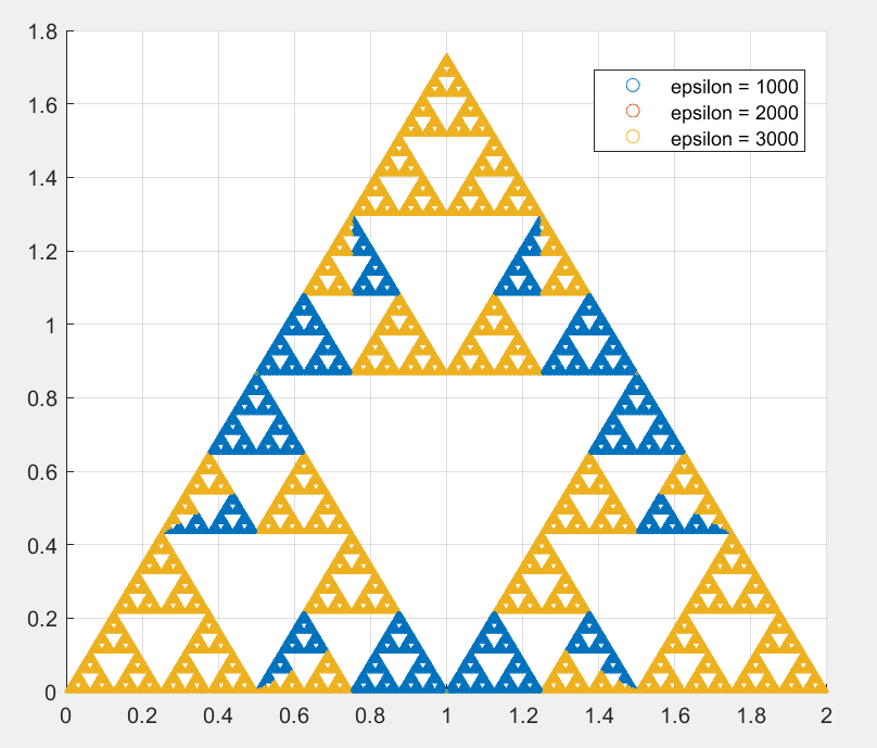
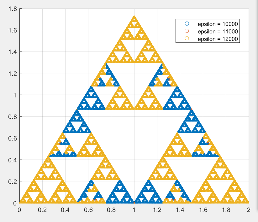
As discussed above, the transition curves are found via -periodic and -periodic Fourier expansions of solutions. However, one might wonder what the curves would be if the same process is undertaken for Fourier expansions of larger periods, say periods . The answer is that curves corresponding to expansions of larger periods in fact ”fill in” the stable regions whose boundary is obtained using the - and -periodic expansions. See Figure 4.1 for an illustration.
In fact, this “fill in” property remains valid for even larger periods, and a proof is given below.
Proposition 4.1.
Let be the set of - pairs such that the corresponding MDE has a solution of period for some . Then is dense in the stable region.
Proof. First, if is a stable pair, then by the discussion given in Chapter VI of [21] we can find two linearly independent solutions and of the MDE, such that
for some . is uniquely determined by the pair , so we may view as a function from the stable region to . In fact, by the Floquet Theorem, there exists a matrix depending only on such that, for any solution of the MDE,
So is a stable pair only if the two eigenvalues of both have norm , which can be written as and . Readers can find details in [21]. Clearly, depends continuously on the parameter , which shows that is a continuous function on the stable region. Next, we fix and , and show that only countably many ’s can be found such that . Recall that for each such we have a solution to the corresponding MDE so that is a -periodic function. We have the Fourier series expansion , which implies
Plugging this into the Mathieu differential equation, we get the following equation for the coefficients,
From this we can see that there are only countably many values of such that the corresponding equation has a nontrivial solution .
Now, we prove the proposition by contradiction. Suppose is not dense in the stable region. Then, there is a ball in the - plane where does not take any dyadic rational value, noticing that when is a dyadic rational the MDE has -periodic solutions for some . This means equals a constant on that ball, since is a continuous function of . However, for this fixed , and a fixed in the ball, there are only countably many possible values for , which can not fill in the ball. This gives a contradiction.
Next we will discuss the asymptotic behavior of the stable and unstable regions. Existing works including [10], [16], and [28] cover two important observations:
-
(i)
First, as illustrated in Figure 4.2, the width of each stable band gets thinner and thinner as tends to . In [28], it is shown that the width of the th stable band will decrease exponentially on as .

Figure 4.2. The width of the th stable band. - (ii)
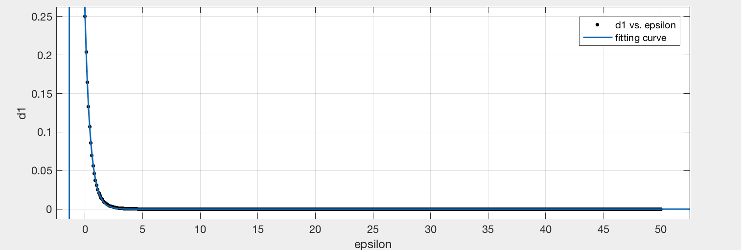
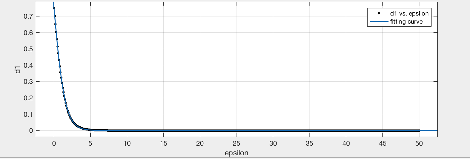
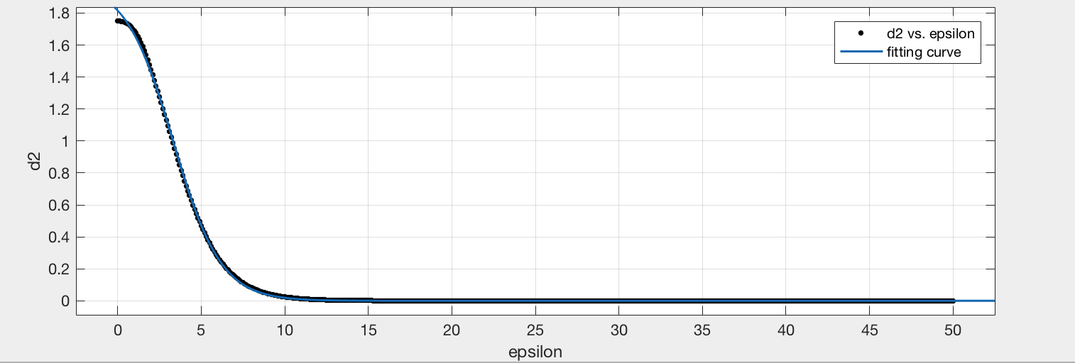
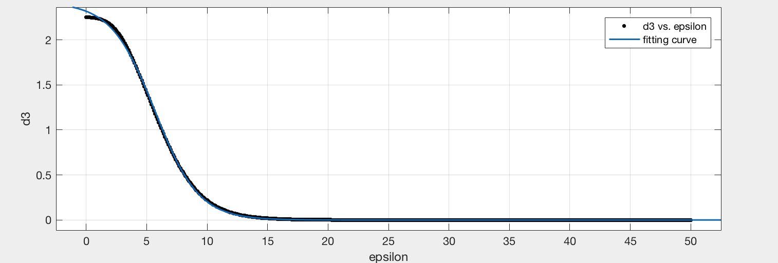
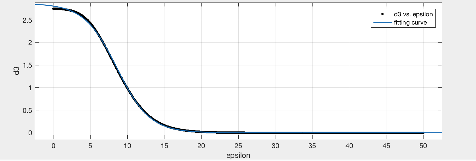
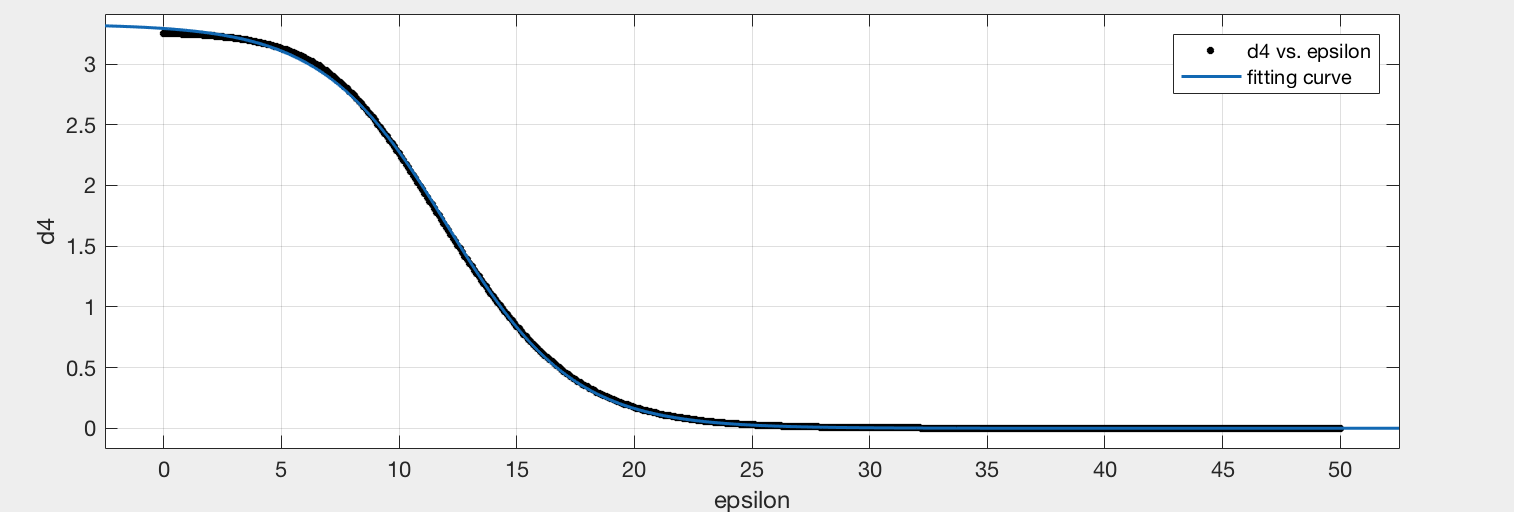
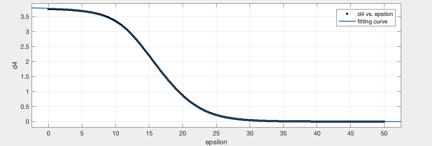
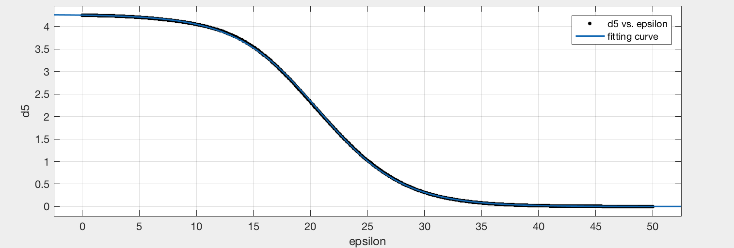
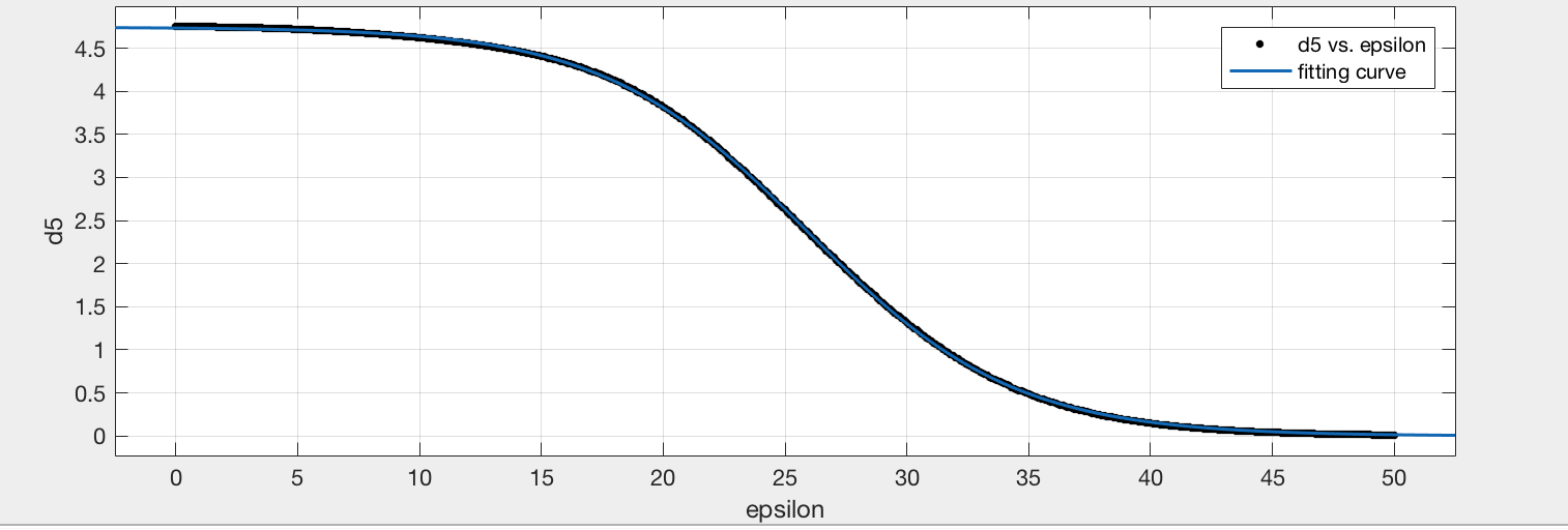
Since the study of the type of convergence in the second observation is comparatively complete, we focus on the type in the first observation, which concerns the width of the stable band as . In particular, we study the first ten stable bands by computing the width of each band from to in increments of . A graph for each stable band, plotting width vs epsilon, are shown below. Then we use the curve fitting toolbox in MATLAB to estimate the fitting curves between and width in each stable band. Please see Figure 4.3 and Figure 4.4 for the result and fitting curves.
Fitting curve of the form: .
 st stable band,
 nd stable band,
 rd stable band,
 th stable band,
 th stable curve,
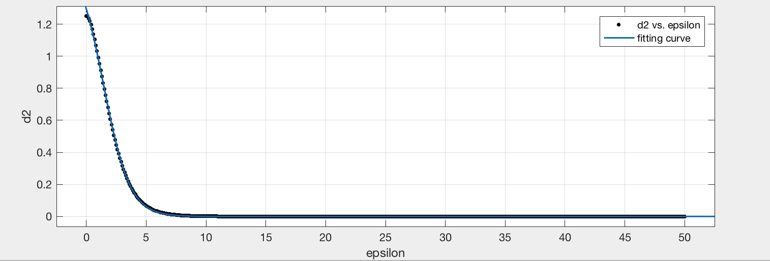
Fitting curve of the form: .
 th stable band,
 th stable band,
 th stable band,
 th stable band,
 th stable curve,
The last topic we will discuss before moving on to talk about solutions to the MDE is to approximate and simplify the irregular boundary between stable and unstable regions for practical use. We can see that most pairs in the first and the fourth quadrants which lie below by the line and above by the line are stable, while most values in those quadrants outside that region form unstable pairs. For any , let . We are interested in determining the probability, for various values of , that a - pair is stable, given that it lies in the triangle So, we numerically compute the probabilities with different choices of . Notice that the line (as well as the line ) alternatively passes through stable and unstable regions. So, we define to be the -coordinate of the point of intersection between the line and the right boundary of the -th unstable region; also, for each we define to be the probability that a - pair is stable, given that it is in . Readers can see figure 4.5 for an illustration of how we divide the regions into triangles.
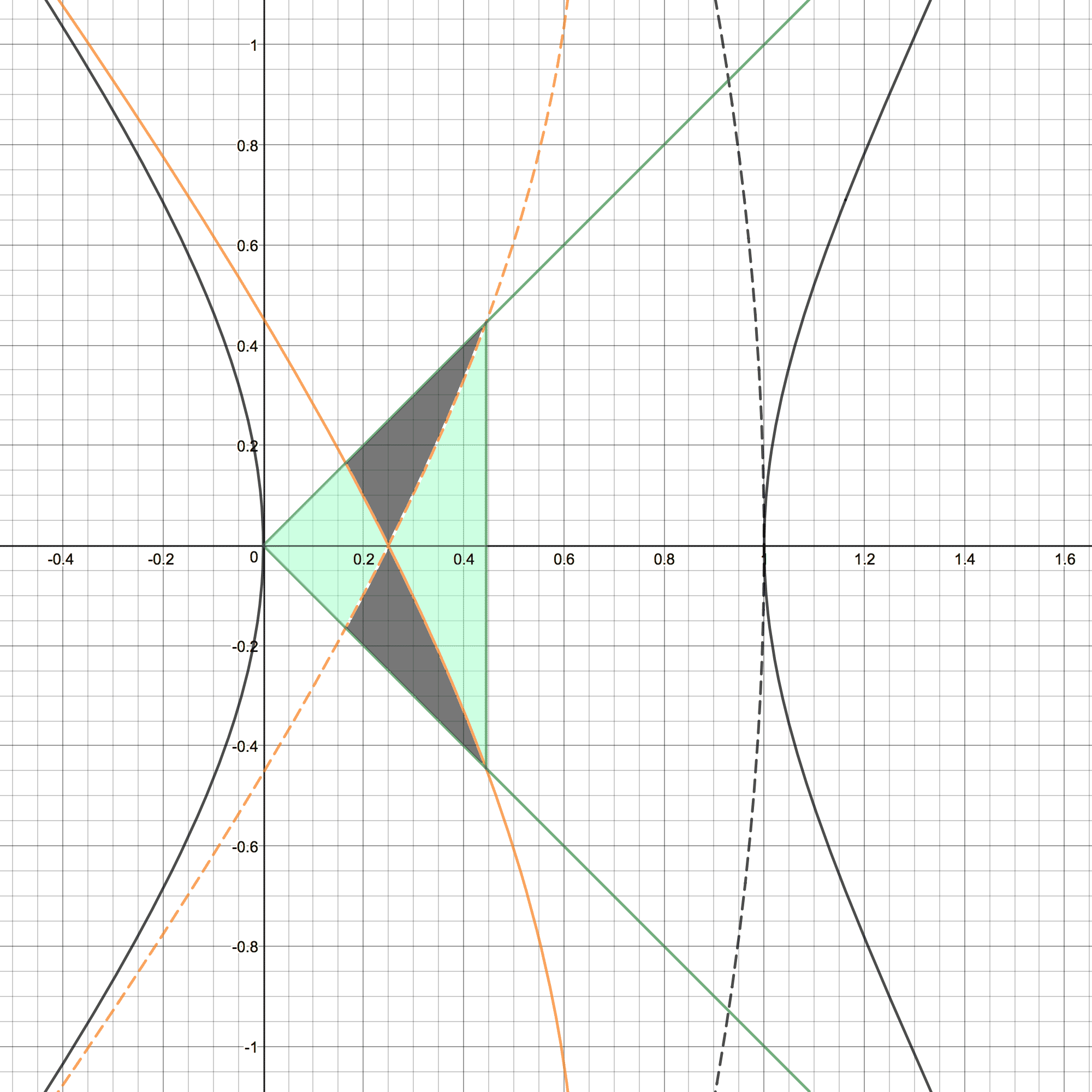
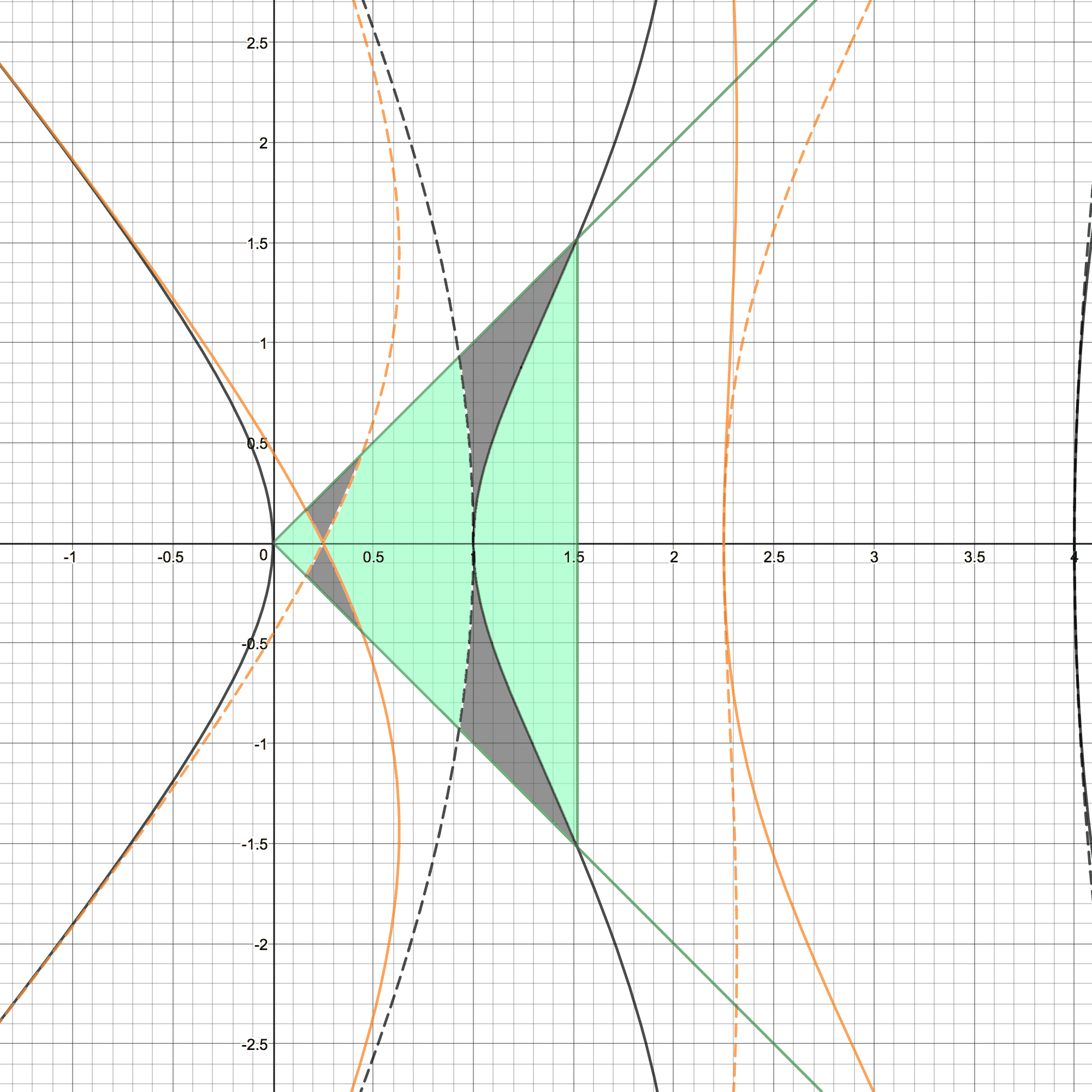
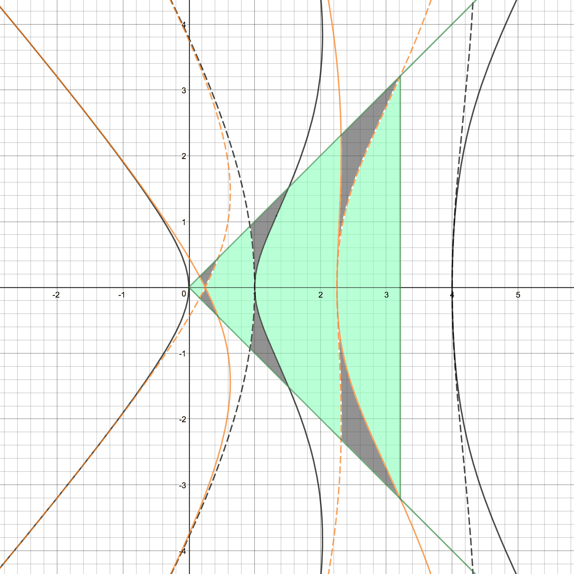
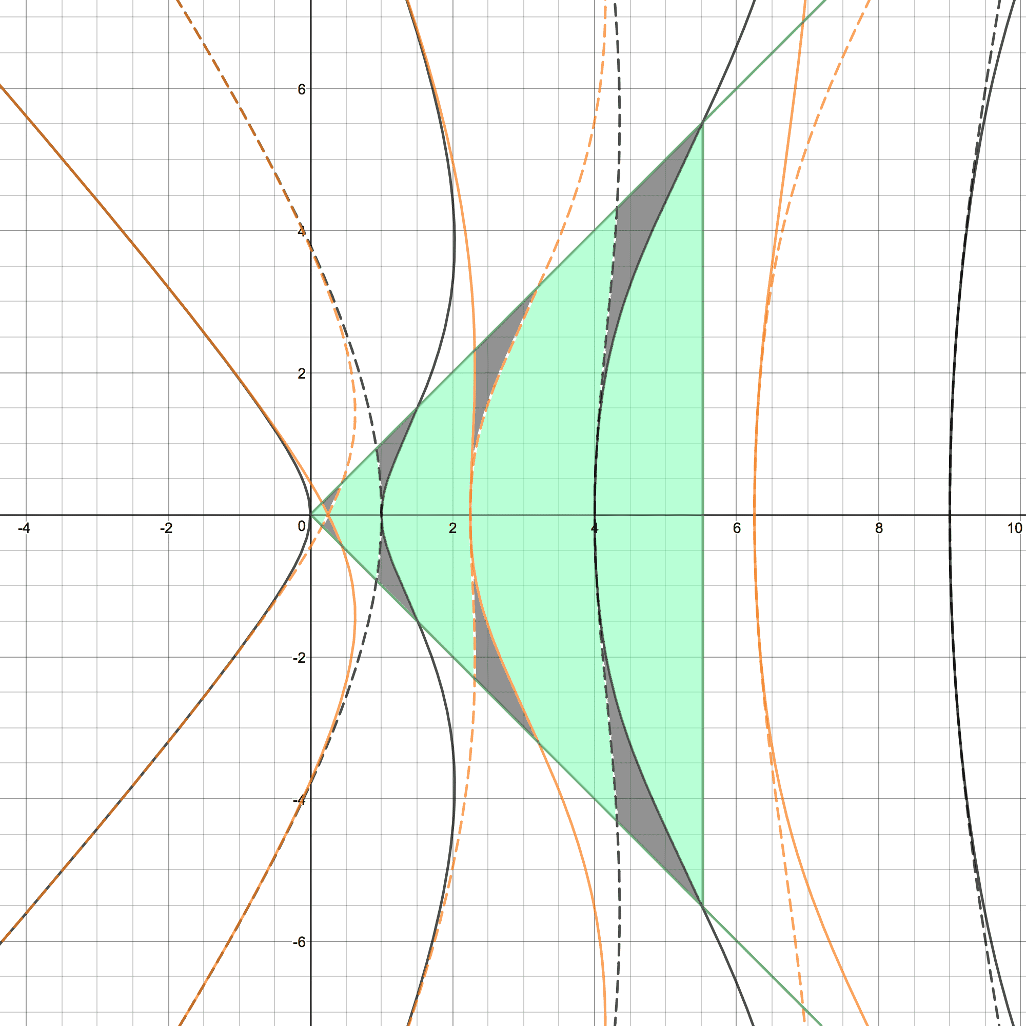
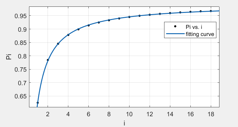
can also be considered as the probability of getting a stable pair within the triangular regions, which can characterize how well the irregular boundaries can be approximated by lines . We list the in Table 1.
| 1 | 0.625056436387445 |
|---|---|
| 2 | 0.784428425813594 |
| 3 | 0.845139663995868 |
| 4 | 0.878143787704672 |
| 5 | 0.899154589232086 |
| 6 | 0.913800056779179 |
| 7 | 0.924632580597566 |
| 8 | 0.932988858616457 |
| 9 | 0.939640860147421 |
| 10 | 0.945067300763657 |
| 11 | 0.949581603650156 |
| 12 | 0.953397960289362 |
| 13 | 0.956667925443240 |
| 14 | 0.959502140424685 |
| 15 | 0.961982968671620 |
| 16 | 0.964174006346465 |
| 17 | 0.966133547589692 |
| 18 | 0.967239011961280 |
In addition, we also obtain a surprisingly good fitting curve of the form , with . See figure 4.6 for details.
4.2. Solutions of the Mathieu Differential Equation
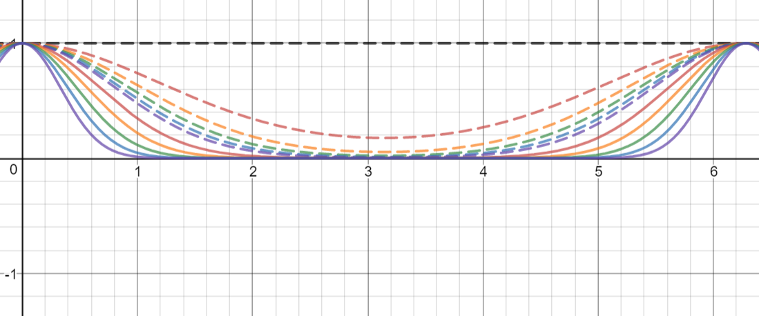
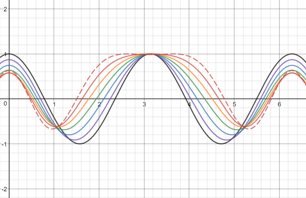
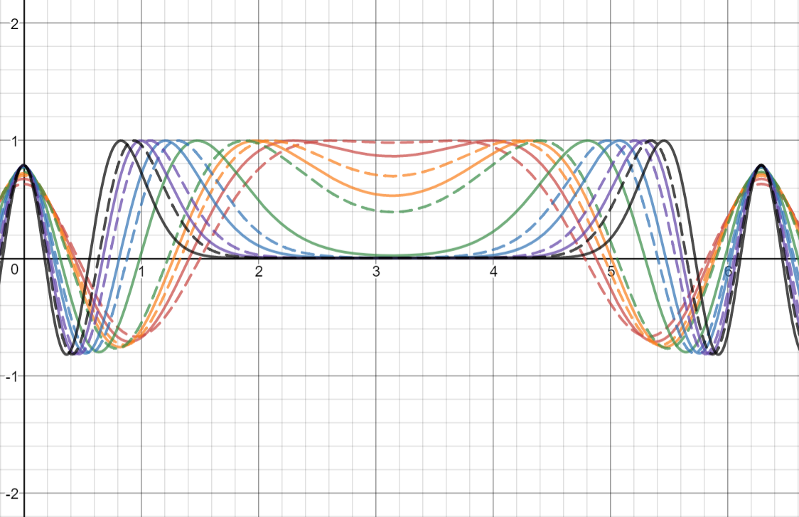
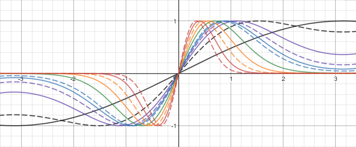
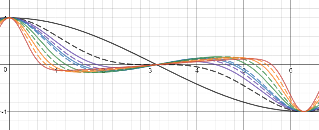
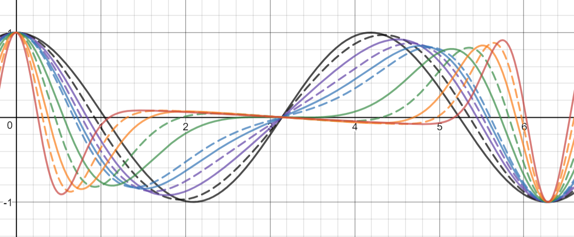
Now we discuss the periodic solutions for the Mathieu differential equation. In Corollary 3.3, we showed that the sequence of Fourier coefficients to periodic solutions corresponding to - pairs on the transition curves converge rapidly. Hence, given a - pair on a transition curve, we can calculate explicitly the coefficients of the corresponding solution with a finite truncation of the Fourier series and use those coefficients to plot, with very high accuracy, solutions to the MDE. One question one might investigate is as follows. Suppose one fixes a transition curve and considers periodic solutions corresponding to various points along that transition curve. How do properties of solutions change as varies? To be more precise, we need some new notation. Recall from Section 2.2 that, when solving - or - periodic solutions, we can rewrite the MDE as a system of linear equations for Fourier coefficents, which collectively can be rewritten as four independent homogeneous matrix equations, with corresponding matrices . The transition curves consist of the - pairs such that one of these matrices degenerates. In this way, a transition curve can be labeled with a matrix and an integer , so that for each - pair on this transition curve, is the th smallest real number such that the matrix degenerates with the fixed . We want a more convenient way to label these transition curves, and to achieve this, we proceed as follows. Fix a transition curve, let on the transition curve, and solve the corresponding equation in matrix form. According to the discussion in Section 2.2, we can then construct a periodic solution to the MDE, and the solution is clearly an eigenfunction of . For example, if we consider the transition curve labeled by and we will get as a solution with the above process. In this way, a transition curve can be labeled with an eigenfunction of . In light of this, we define to be the point in the - plane with prescribed -coordinate which lies on the transition curve corresponding to the eigenfunction . As shown in Section 2, the transition curves can be organized into four different classes, made up of points with our new notation. It is natural to study them separately. First we consider the class . Because of the symmetry of the transition curves across the -axis, it suffices to only consider positive values of . In fact, if is a solution corresponding to the pair , then is a solution corresponding to the pair since . The normalized solutions are plotted in Figures 4.7-4.9, where by ‘normalized solution’ we mean a solution for which . In plotting the graphs we have used the particular values and . truncated matrices are used to compute the solutions. The horizontal axis is the -axis, and the vertical axis is the -axis.
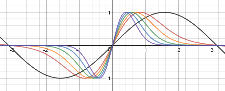
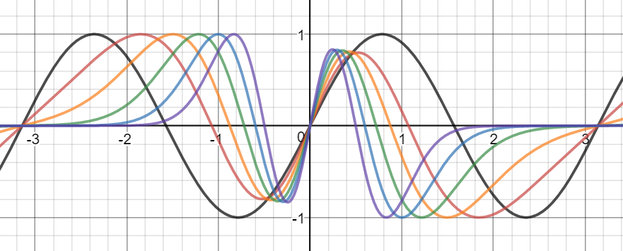
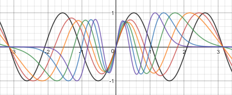
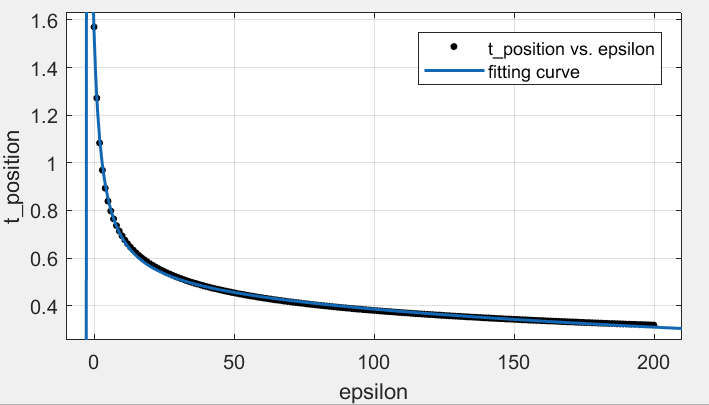
An interesting pattern can be observed from Figure 4.7. The sequence of -coordinates of these maximal points appears to approach monotonically as increases. Figures 4.8 and 4.9 show the same behavior as well. We now use curves to fit a curve of the -coordinate of these relative maxima in as a function of . We still pick the same three transition curves, and take from to , in increments by . The relationship of coordinate of maximal points and on the three curves are shown in figure 4.10, and the fitting curve is of the form .
-position of maximal point on curve , with .
-position of maximal point on curve , with .
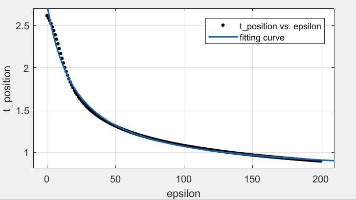
-position of maximal point on curve , with .
For the case of and , does the same convergence behavior occur if one considers the sequence of the first minima when ? We also do the computation, and show the results in figure 4.11, where the same kind of fitting curve also works.
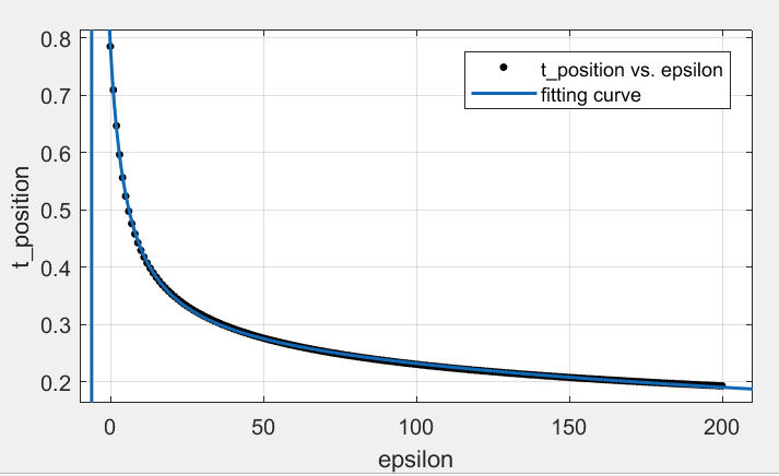
-position of the second maximal point on curve , with .
-position of the second maximal point on curve , with .
In case of , the same observation applies to the second maxima when . See figure 4.12 for details.
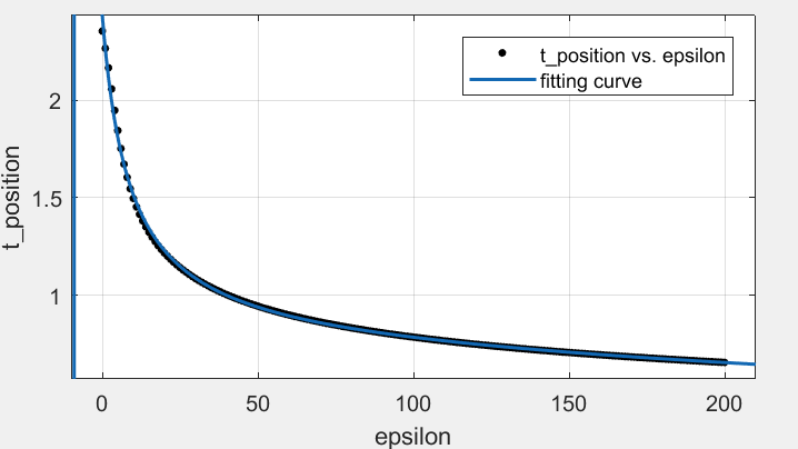
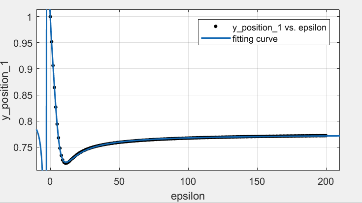
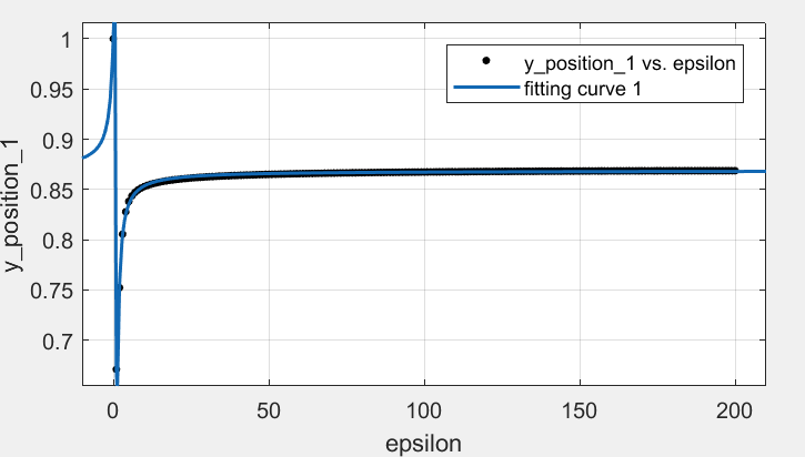
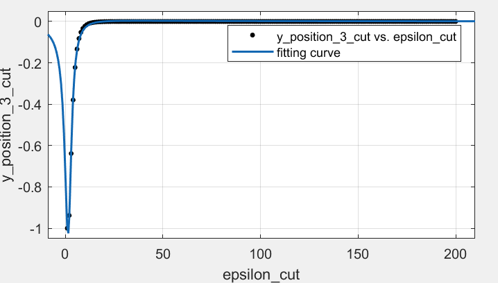
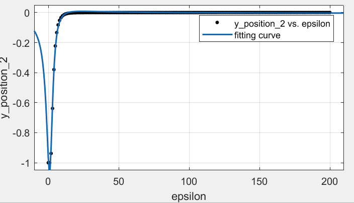
One can also consider the behavior of the -coordinate of these various sequences of local extrema. See figure 4.13 for the behavior of -coordinate of the first minimal points on the curve , where we can fit the points well with a rational function of the form .
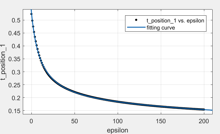
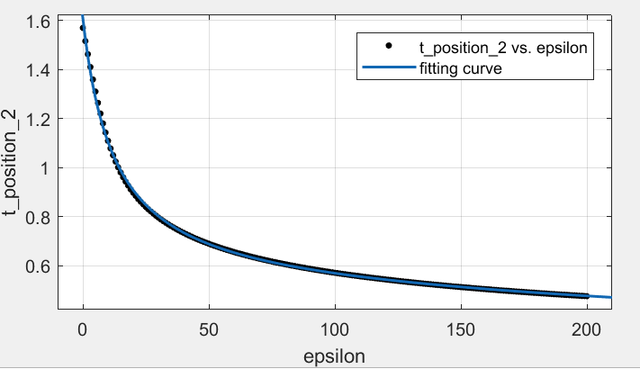
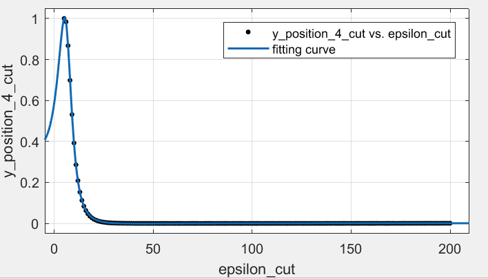
For the curve , there are three local extremes on each solution, and we also do the computation for the -coordinate for the first minimal and the second maximal value. The fitting curve is a little more complicated, of the form . See figure 4.14.
-position of the second maximal point on curve , with .
-position of the third maximal point on curve , with .
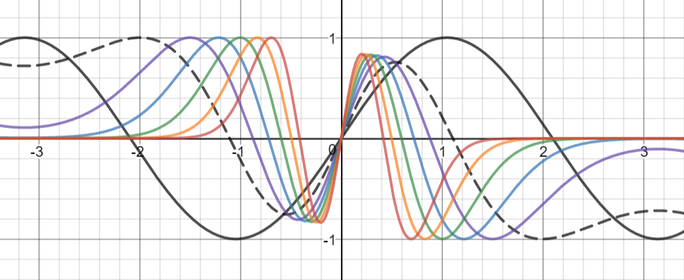
Next, we turn to the solutions on curves , and we do experiments for . Please look at figure 4.15,4.16,4.17 for the results.
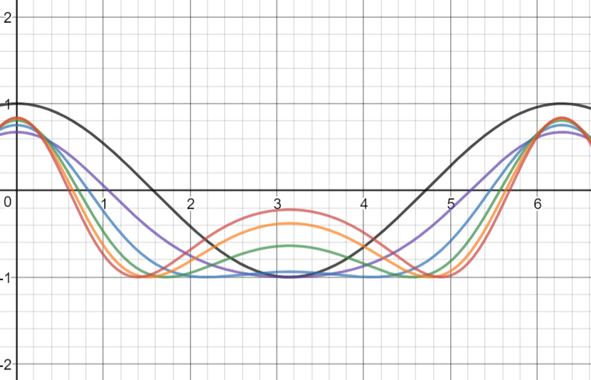
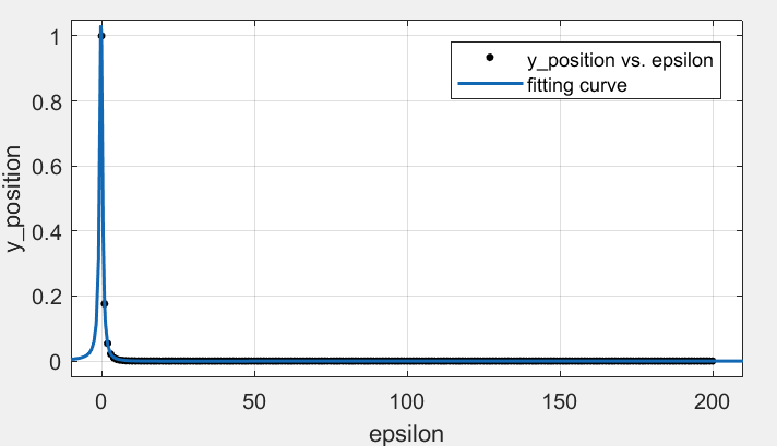
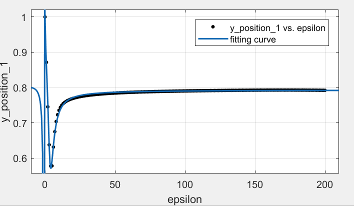
We can see that the shapes of these curves are different from those in figure 4.7 4.8,4.9. The first curve is of course very special, as it corresponds to the constant functions. It turns out the solution is always positive on this curve, as a consequence of Sturm’s Theorem [17]. Also, we have the minimal values of the solutions at , see figure 4.18 for the minimal values for different choices of . We use a fitting curve of the form .
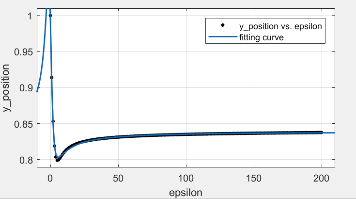
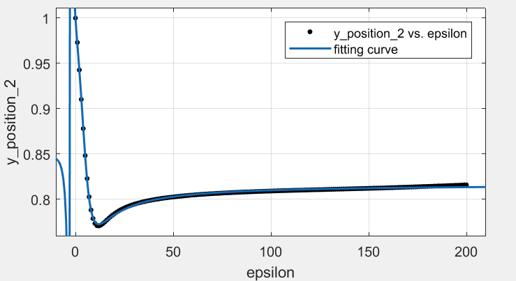
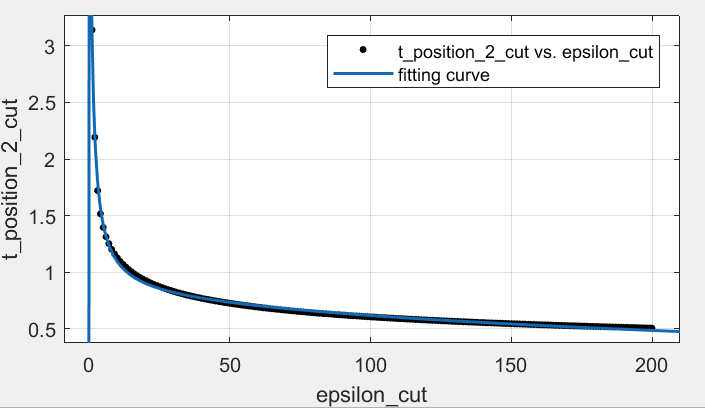
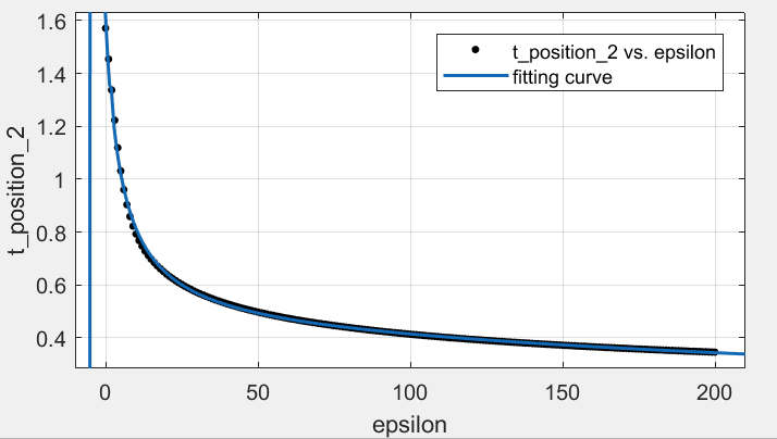
The solutions on the second curve is a little more complicated. As shown in figure 4.16, we can see that minimal value is achieved at in for and , but as becomes larger, the minimum point splits into two different minimum points. This is an interesting phenomenon, and we have an explanation for this in Theorem LABEL:thm44. We do computations on the -coordinate of the minimum points as gets larger. Please see figure 4.19 for the data, and we use a fitting curve of the form .
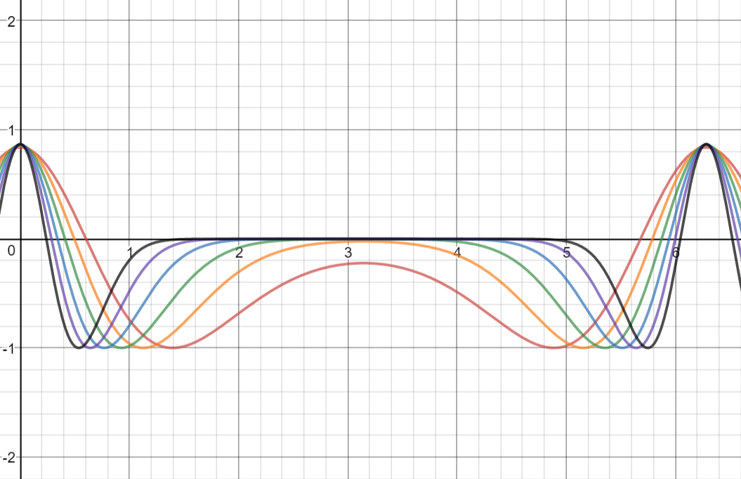
Another thing we need to highlight here is that the maximal absolute value does not occur at or , but at some other points. So, as usual, we normalize the solutions so that their minimum value are , and we compute values of solutions at the two other local peaks at and , which is shown in figure 4.20. It is also interesting to see in figure 4.21 that the local maximal value at drop rapidly near , and then increase quickly.
The solutions on the curve is even more complicated. Still, we observe the split of one peak. When , we only see one maximum point, but as becomes larger, we see two maximum points. We also do computation on the coordinate of one of these splited maximum point. See figure 4.22 for the computation result, where we use fitting curves of the form .
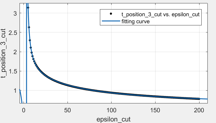
We also do experiment on the t coordinate of the first minimum points and the -coordinate of the peaks on the curve .
4.3. Explanation on the Behavior of the Solutions
Before the end of this section, we give a proof on the convergence of the t-coordinates of the peaks. This interesting point is that the behaviors are closely related to the asymptotic behavior of the transition curves, i.e. how behaves as increases to . There are several works on this problem, and here we refer [17] for one version. Readers can find other dicussions in [28].
Theorem 4.2 (W.S. Loud).
For fixed , let be the th smallest value on the transition curves. Then we have
as . ∎
Notice that in the above theorem, we fix a transition curve and let , which is exactly the way we study the behavior of the solutions. Now, we apply the theorem to derive some interesting facts that we have observed in our experiments.
Lemma 4.3.
For fixed , let be the th smallest value on the transition curves, and be a nontrivial periodic solution for the corresponding MDE. Then, for large , there is no local extremum of in where .
Proof. Let be the zero of in , where theorem 4.2 guarantee the existence of when is large. In addition, we have the estimate by using Taylor expansion of locally at ,
(b) We only need to understand the behavior of at . The idea is essentially the same as the proof of Lemma 4.3, where we look at the sign of . It is also clear that and in this case. Notice that , and we set by multipling a constant, so that we can conveniently look at the absolute value of . If , then is a local maximum of ; if , then is a local minimum of . For the case that , we can see that on except for the case , which only happens on the curve characterized by . So is still a local maximum of . In addition, is a strictly decreasing function of on , so we can find a critical point such that on , and on . To show that is strictly decreasing, notice that is the th smallest value such that the MDE has a - or -periodic solution, which is equivalent to say that is the th smallest eigenvalue of the self-adjoint operator on . Let , and be the corresponding eigenvalues. Then using Raleigh quotient, we get
where is the space spanned by the smallest eigenfunctions of and the infimum in the last line is taken over all the dimensional subspaces of on .
Remark. In Theorem 4.2, Lemma 4.3 and Theorem 4.4, we considered the case that . Since , for the case that , the MDE can be rewritten as
with . We can still use Theorem 4.2, Lemma 4.3 and Theorem 4.4 to study solutions to the MDE with coefficient , by applying a shift of .
5. The Sierpinski Gasket and the Fractal Laplacian
In this section we give preliminary definitions and results concerning analysis on fractals and provide a basic introduction to the ‘infinite’ Sierpinski gasket will be given. This serves to set up the discussion of the generalization of the MDE to the fractal setting described in in Section 6.
5.1. Sierpinski Gasket
Consider the three contraction mappings given by
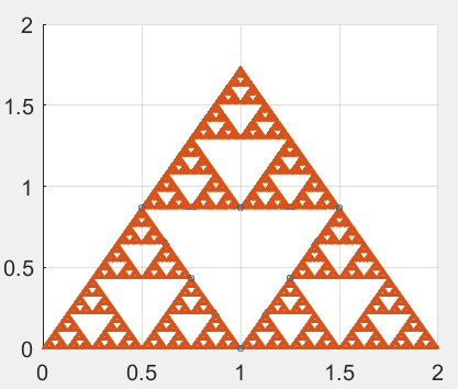
where . Then form an ‘iterated function system’ (see page 133 of [7]). By Theorem 9.1 in [7], there exists a unique nonempty compact set such that (see [11])
Then is defined to be the Sierpinski gasket, often denoted . See Figure 5.1.

In studying it is useful to use its graph approximations, constructed as follows. Let and be the unique fixed points of and respectively. Define a vertex set . Then ,for any . We refer to as the boundary of . We further define vertex sets for inductively by and let be the set of all vertices. Note that is dense in . For an -tuple , where for each , we define by
and say that is a word of length . With this, an edge relation on can be introduced as follows: for we say if and only if there exists a word of length and unequal indices such that and . This relation on gives a sequence of graphs approximating SG, with the vertex set and the edge set . See Figure 5.2 for .


5.2. Fractal Laplacian
Now we are ready to define the Laplacian on . Suppose We define the level- discrete Laplacian by
Then we define the continuous Laplacian by
If the limit above converges uniformly on to a continuous function, we say . In this case, we extend to all of , including points not in , by continuity (recall that is dense in ). The continuous Laplacian on SG is the analog of the usual ‘second-order derivative’ on the line.
We shall mention now the the following proposition derived by O. Ben-Bassat, R.S. Strichartz,and A. Teplyaev in [3], which will be of interest in the next section.
Theorem 5.1 (O. Ben-Bassat, R.S. Strichartz & A. Teplyaev).
Let be a nonconstant function in dom Then is not in dom. ∎
A function satisfying for some number is called an eigenfunction of with eigenvalue . If a function satisfies then we say that satisfies the Dirichlet boundary condition, and the eigenvalue problem
is called the Dirichlet eigenvalue problem. A function satisfying both of these equations is called a Dirichlet eigenfunction of Similarly, we have a notion of a ‘Neumann condition’ as follows. Define the normal derivative for by
where we have identified indices modulo 3. If a function satisfies for and then we say that satisfies the Neumann boundary condition, and the eigenvalue problem
is called the Neumann eigenvalue problem. A function satisfying both of these equations is called a Neumann eigenfunction of Dirichlet and Neumann eigenfunctions on are the analog of sine and cosine functions on the line.
5.3. Spectral Decimation
A method for explicitly computing all possible eigenvalues and eigenfunctions of was introduced in [8] using a process called spectral decimation. Below we briefly discuss some results from spectral decimation we will use. Readers can find detailed discussion on spectral decimation in [8] and [22].
Proposition 5.2.
Suppose , and is given by
| (5.1) |
(a) If is a -eigenfunction of on , then it can be uniquely extended to be a -eigenfunction of defined on . (b) Conversely, if is a -eigenfunction of on , then is a -eigenfunction of on .
If we want to extend an eigenfunction of with eigenvalue to an eigenfunction of using the proposition above, we have two choices, except when (as we will see below), in which to extend the eigenfunction:
For convenience, define the functions and by
The numbers are called forbidden eigenvalues, and it turns out that each Dirichlet eigenfunction of comes from a 2-, 5-, or 6-eigenfunction of for some , while all the Neumann eigenfunctions come from 5- or 6-eigenfunctions of for some . If is a Dirichlet or Neumann eigenfunction, we call the generation of birth and the initial function. Suppose is an eigenfunction of with eigenvalue arising from initial eigenvalue Then we say that is a 2-series (resp., 5-series or 6-series) eigenvalue if (resp., or 6). With a fixed generation of birth and initial function , we can extend the function level-by-level. We can first fix a sequence of , with only finitely many , and then let for inductively. Then the function is extended to be an eigenfunction of , with the corresponding eigenvalue
In fact, all the eigenfunctions with a given generation of birth and initial function can be generated by the above recipe. Also, if the initial eigenvalue is , we can only choose , as is a forbidden eigenvalue. Now, suppose we fix a generation of birth , fix an initial function on , and let
where denotes the empty sequence. Define , where is the length of . In particular, . Let . Then, we can deduce the following possibilities: 1. If or , then all the possible eigenvalues of having generation of birth are given by
2. If , then all the possible eigenvalues of having generation of birth are given by
Here we remark that when we use the notation , we always assume that we have a fixed generation of birth and initial eigenvalue . There is a method, given by [5], in which to arrange in increasing order the set of eigenvalues arising a fixed generation of birth and initial eigenvalue. The idea is to translate each finite sequence in into a binary number. The process is as follows. Given of length , let be the integer with binary (base-2) expansion , where
In addition, we set . Then is the -th smallest eigenvalue. For example, if , then where is written in base-2. Thus, corresponding to the sequence is the 105th smallest eigenvalue. Also, note that, in particular, is the smallest eigenvalue, is the 2nd smallest eigenvalue, and is the 3rd smallest eigenvalue. We can, of course, reverse this process so that, given an in integer we can find the corresponding to the -th smallest eigenvalue. Another fact is that the sequence of eigenvalues , where , corresponding to a fixed generation of birth and a fixed initial eigenfunction grow according to the power law . In addition, if we define the eigenvalue counting function to be
then we have the following proposition concerning the asymptotic behavior of .
Proposition 5.3.
For a fixed generation of birth and fixed initial function on , there exists a -periodic continuous function such that
Proof. To avoid the high multiplicity of eigenfunctions corresponding to a same eigenvalue, we fix an initial eigenfunction instead of just fixing an initial eigenvalue. In our setting, the eigenfunction is unique for each eigenvalue, so we only need to count the number of eigenvalues. For convenience, we prove the proposition for generation of birth and initial eigenvalue . For initial eigenvalue and , the arguments are essentially the same. We will show that converges to uniformly on some interval as . First, we have the following observations. Observation 1: For eigenvalues of generation of birth and initial eigenvalue , if is fixed then we have
for all where for each word . Notice that , and the fact , we have . The observation follows. For each , we denote the endpoints of by and , i.e., . By some easy computation, we can get the following observation. Observation 2: Assume . Then
To show observation 2, we need to consider two cases. First, for any with , we have , which counts for eigenvalues. Second, we have eigenvalues in each interval of the form , where . In fact, for , if and only if , and we have free choices for each . There are intervals in , noticing that if and only if . Combining the above facts, we get the second term . Now, fix and consider . It is easy to see that converges as , since it is a constant for . We denote the limit . Next, we look at general . Note that we can find some constant such that
since . We want to show that converges to some function uniformly on as . In fact, if we fix and look at for some such that , we have
for any . In addition, if , we have
where . Similarly, we have for ,
where . The above discussions shows that converges to some function uniformly on as . Also we can easily see that is continusous with from the estimates. In fact, for each , we can find a small neighbourhood such that for and any in the neighborhood, . The estimate obviously holds for the limit function. We can extend to be periodic on , and the theorem follows immediately.
5.4. Infinite Sierpinski Gasket
In the last part of this section, we introduce the infinite Sierpinski gasket (). It is a particular example of fractal blow-ups introduced in [24] by R. S. Strichartz.
Recall that the Sierpinski gasket is defined by the self-similar identity, , where each is a contraction mapping of contraction ratio for , as defined earlier in this section. The infinite Sierpinski gasket is constructed as follows.
Definition 5.4.
Suppose a sequence , , is fixed. Define , where . Then the infinite Sierpinski Gasket is defined by . ∎
The Laplacian on can be defined locally with graph approximation in a same way as on . In [27], a Sierpinski lattice was introduced to describe the infinite graphs that approximate . Define
and say if for some . Then the resulting infinite graph is called a Sierpinski lattice. We can still define the discrete Laplacian on the lattices by
Then the continuous Laplacian is defined by
One of the most important results on was A. Teplyaev’s theorem (see [27]) below showing that the Laplacian on has pure point spectrum, which means the eigenfunctions of the Laplacian form a complete set.
Theorem 5.5 (A. Teplyaev).
The Laplacian is self-adjoint in , where is the Hausdoff measure on . The spectrum of is pure point (i.e., the eigenfunctions of form a basis of ) and each eigenvalue has infinite multiplicity. The set of eigenfunctions with compact support is complete in . ∎
As a result of the theorem, spectral decimation still works on . Each of the eigenfunctions of is an extension of an eigenfunction of with eigenvalue or by spectral decimation. The only difference here is that the generation of birth takes values in instead of . All the results concerning eigenvalues from a same generation of birth and initial function in the previous section, including Proposition 5.3, still hold on .
6. Extending the Mathieu Differential Equation to Infinite Fractafolds
Now we are ready to discuss how we will define the Mathieu differential equation on an infinite fractafold.
6.1. Defining the Fractal MDE
Recall that the MDE, defined on the real line, is given by
where is a function from to . The first questions we wish to address are “What should the fractal space be that replaces the line?” and “what should ‘periodic function’ mean?”. We choose to consider the infinite Sierpinski gasket to be our domain. By “periodic function,” we mean a function on which is identical on all the copies of of the same size. In particular, if we are given a function on with the boundary conditions
| (6.1) |
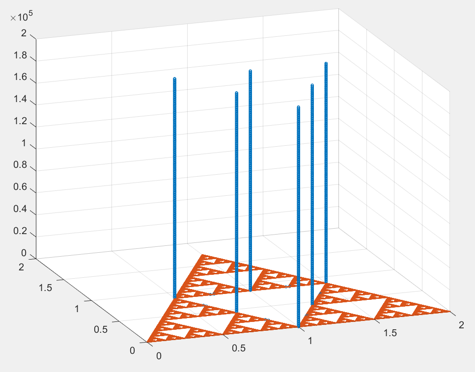
we can get a periodic function on by translating the function to other copies. But what about the differential equation? The first step in finding a fractal analog of the MDE defined on the line is to replace with the fractal Laplacian , since is the analog of the second-derivative operator. Now, what to do with the term? Recall from Theorem 5.1 above that the multiplication of two nonconstant functions in dom may result in a function which is not in dom. Thus, we cannot simply replace by a function in dom, and so we must figure out a suitable analog of multiplication by cosine. Recall that, in the line case, we sought solutions in the form of a Fourier expansion in terms of cosines and sines. Note, however, that cosines and sines on the line are Neumann and Dirichlet eigenfunctions, respectively, of . Hence, we will adopt a form of Mathieu’s equation which is compatible with functions that can be written as a linear combination of Neumann eigenfunctions, motivated by Equation (6.1). We choose to only consider functions which have Neumann eigenfunction expansions of the form
| (6.2) |
where each is a Neumann eigenfunction function defined as follows. Fix a generation of birth, a series (5-series or 6-series), and an initial eigenfunction such that for all and . With the spectral decimation algorithm introduced in Section 5.3, we obtain a set of Neumann eigenfunctions of extended from , and we write for the eigenvalue corresponding to . We still take the order as in Section 5.3. Readers can also find more details on Neumann eigenfunctions on in [22]. The reason we fix a common initial Neumann eigenfunction is that, if we do not fix such an initial eigenfunction and instead consider the set of all Neumann eigenfunctions of , then we cannot order their eigenvalues in a discrete way as above. To this end, suppose we have a function on which can be written as a linear combination of Neumann eigenfunctions as in Equation 6.2, where the () satisfy the definition in the previous paragraph. Then, for any with we define multiplication by cosine as follows:
The motivation for this definition comes from the fact that, for the line case, the Neumann eigenfunction obeys the following trigonometric property when multiplied by :
As for we consider two possibilities, each of which will be described in Section 6.2. In addition, we will consider another two variant versions in the following subsection. Using our developments thus far, the fractal Mathieu differential equation would say
where is the eigenvalue of corresponding to eigenfunction . Since the set of eigenfunctions is linearly independent, we must have
| (6.3) |
Putting these equations into matrix form we obtain
| (6.4) |
Note that this matrix takes the form of Equation 3.1, which reproduce below:
6.2. Variants of the Mathieu Differential Equation on the Line
We will consider 4 different ‘versions’, , , , and , of the coefficient matrix for the fractal MDE ():
-
•
Version 1:
This matrix is reminiscent of the cosine matrices for the line case. Note that the first term in the second row is , not . The recursion relation for the coefficients becomes
(6.5) -
•
Version 2:
This matrix is reminiscent of the sine matrices for the line case. Note that the eigenvalues start from instead of . The recursion relation for the coefficients becomes
(6.6) -
•
Versions 3 and 4: For Version 3 and for Version 4 we take the following approach. We now consider a variant of the Mathieu differential equation, given by
where is the operator analogous to multiplication by cosine. For , define with and satisfying
(6.7) for . One can solve system 6.7 to find the solutions of and
(6.8) Note that and for all , and hence the sequences and are each uniformly bounded. The motivation for the setup above is that, if we plug in , which corresponds to the eigenvalues on the line, Equation 6.8 yields . For and , we still consider two cases, which give us Version 3 and Version 4 as follows. We let Version 3 be
where and are as given in Equation 6.8. This matrix is reminiscent of the cosine matrices for the line case. Note that the first term in the second row has an extra factor of . The recursion relation for the coefficients becomes
(6.9) We let Version 4 be
where and are as given in Equation 6.8. This matrix is reminiscent of the sine matrices for the line case. Again, note that the eigenvalues start from instead of . The recursion relation for the coefficients becomes
(6.10)
7. Ovservations and Analysis for the Fractal Mathieu Differential Equation
In this section we parallel our results presented in Section 4 by giving a discussion of the asymptotic behavior of the transition curves (defined below) for the fractal MDE and of the convergence of solutions. We also describe a phenomenon wherein the transition curves form a prominent ‘diamond’ pattern.
7.1. The - Plot
In Section 6, we introduced 4 different Versions , () of the fractal MDE in matrix form on . If one fixes one of the four Versions of the MDE as above, then the points in the - plane for which the has a nontrivial solution in make up the transition curves for that Version of the MDE. In Figures 7.1-7.8, we show the transition curves for each of the four Versions.
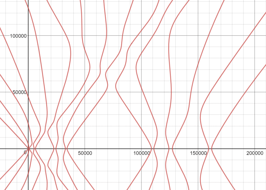
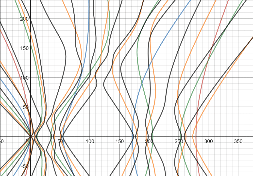
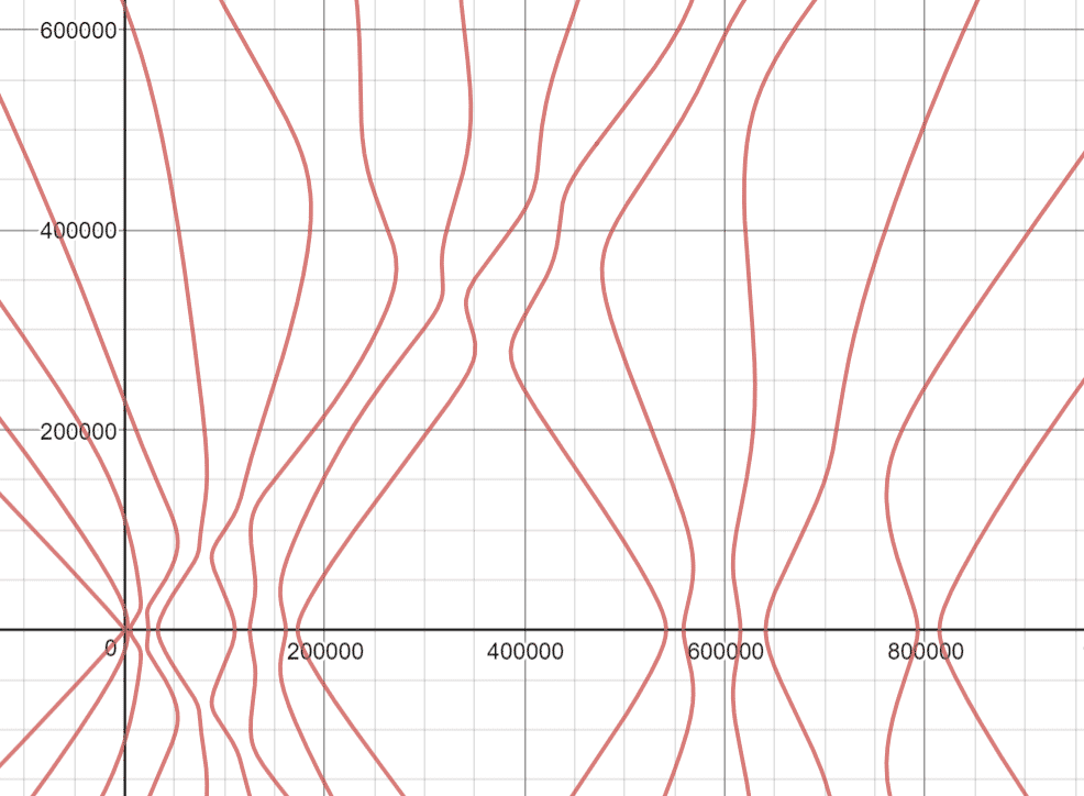
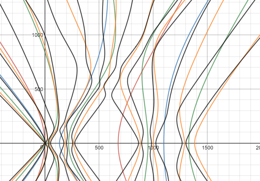
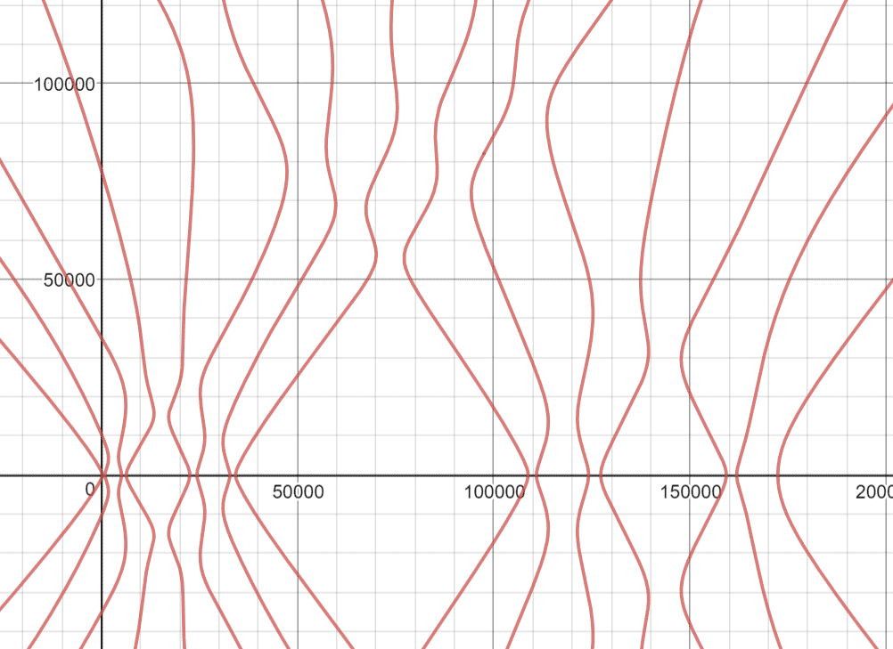
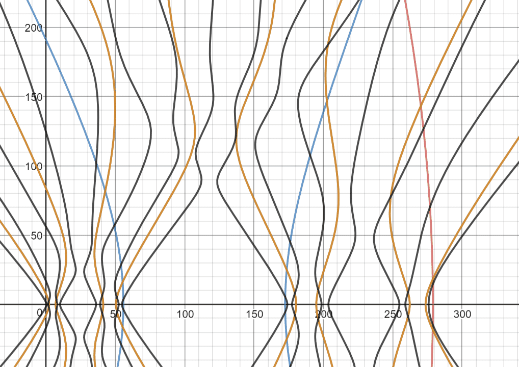
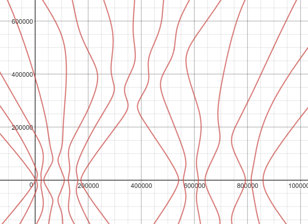

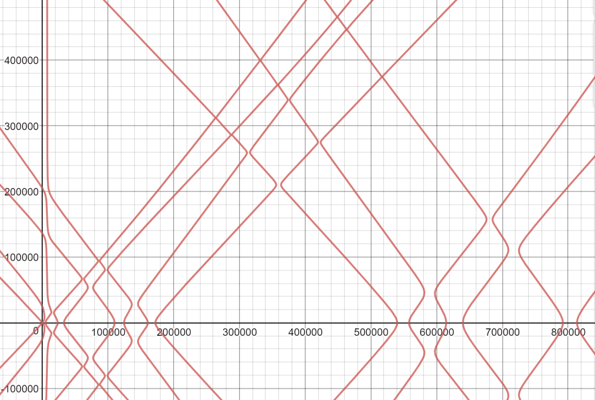

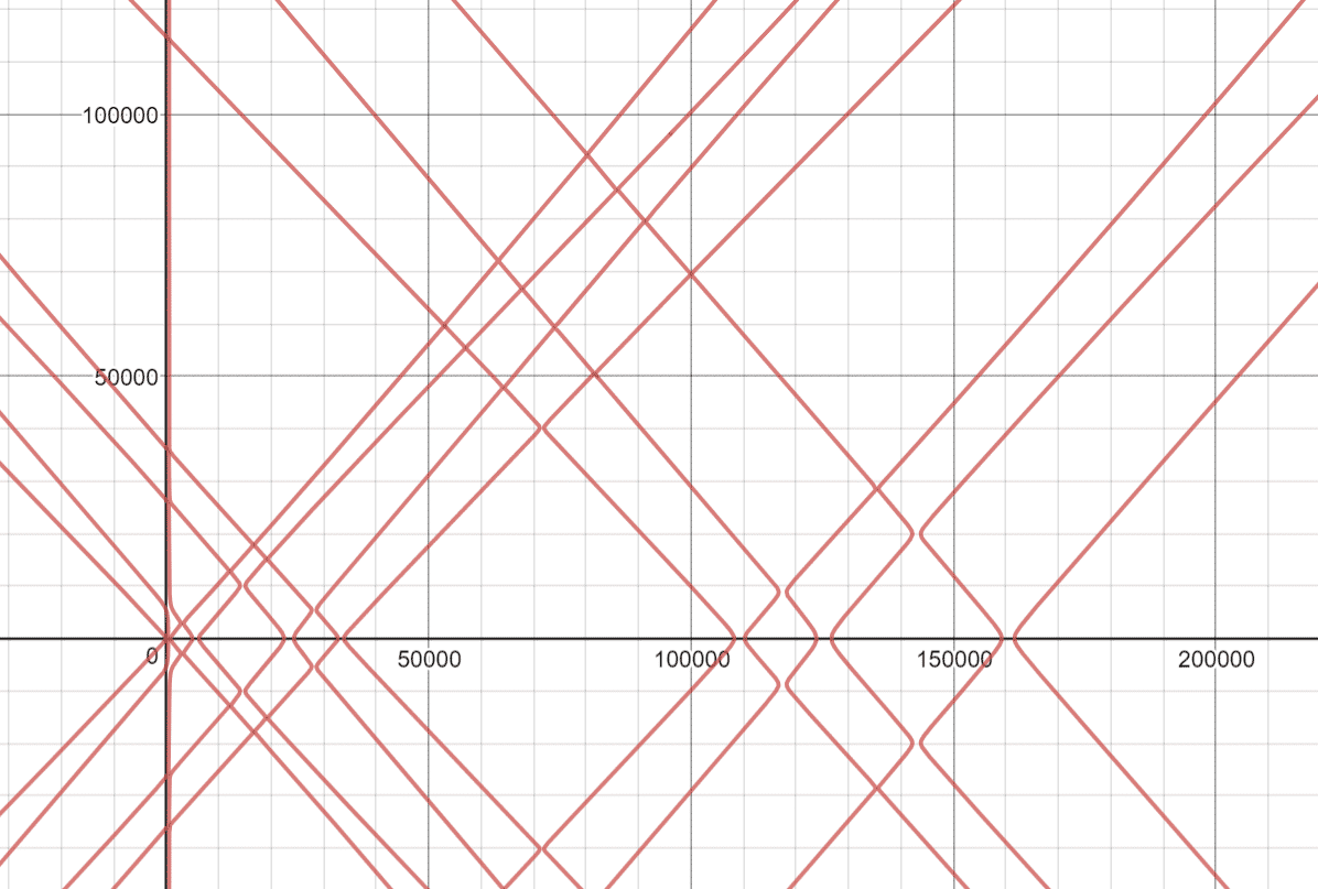
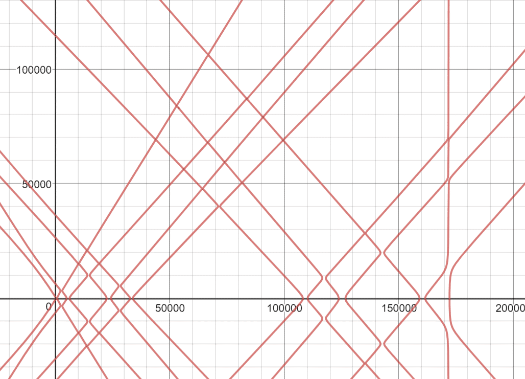
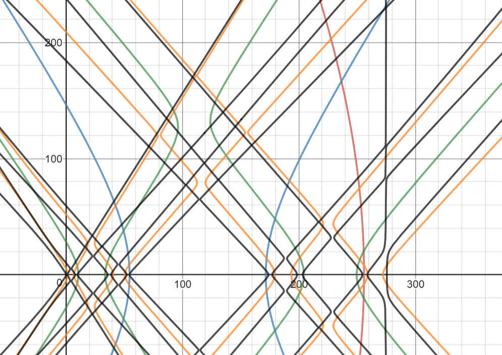
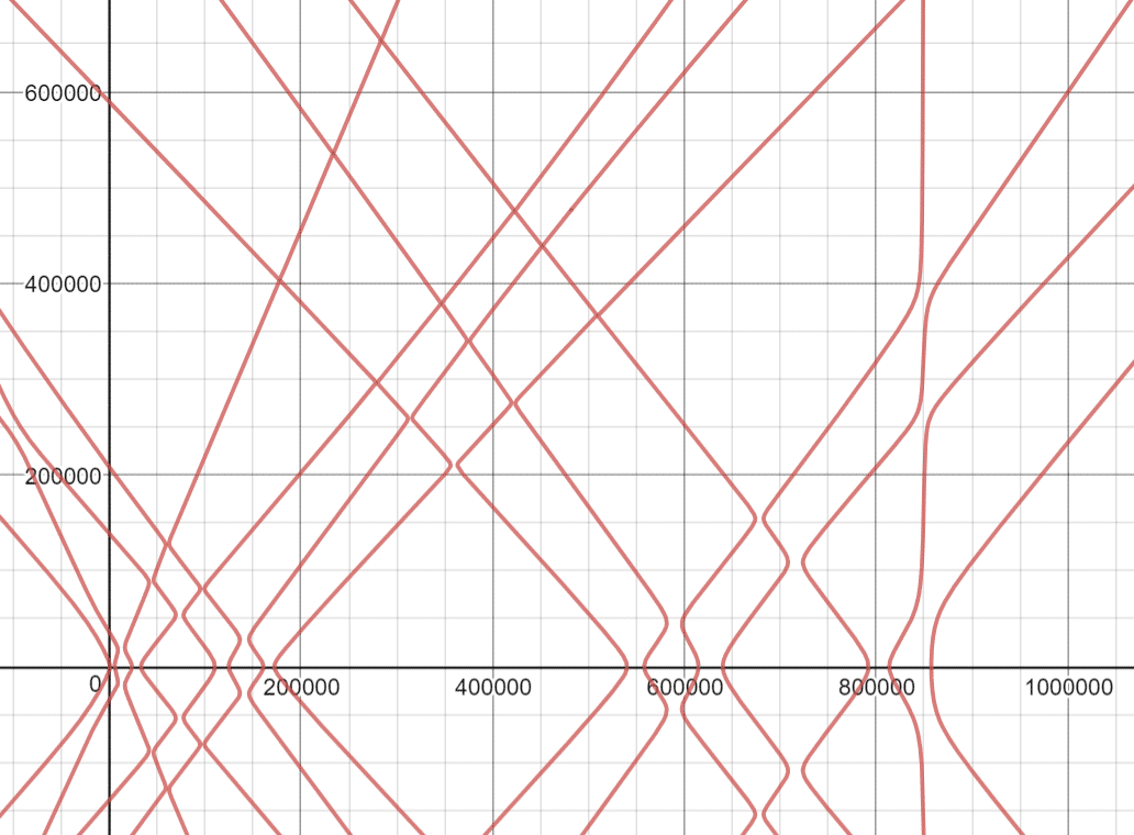

As can be viewed from Figures 7.1-7.8, in each plot there is a ‘diamond’ pattern formed between adjacent transition curves. That is, the curves seem to ‘bounce’ off each other before parting in separate directions. This pattern does not appear in the transition curves for the Mathieu differential equation on the line. This is one way in which the transition curves for are different than those for the line. We give a short proof here concerning the asymptotic behavior of the transition curves for Versions 1 and 2.
Proposition 7.1.
For version 1 and version 2, fix one transition curve. The ratio converges to if . The ratio converge to if .
Proof. In fact, and are of the form , where is a diagonal matrix, and has one of the following two forms,
The first matrix is real symmetric with continuous spectrum . To see this, we only need observe that , where is defined as . The second one is not symmetric, but we can study the matrix where is a diagonal matrix, we did in the proof for theorem 4. After the transformation, we have
which is also a real symmetric matrix with continuous spectrum . Without loss of generality, we just assume is symmetric in the follows. In the following proof, we only consider case, and the other half is then immediate by symmetry. On the -th curve, we know that
where the infimum takes over all the dimensional subspace of dom. It is easy to see the following lower bound of
Next, we give an upper bound. For any , we can find a dimensional subspace , such that , which means
In fact, observe that has continuous spectrum , we can always find a dimensional subspace such that . But is not necessarily in . So we pick a large , and define
Obviously, , and as long as is large enough. Then we get the following upper bound
Combining the upper and lower bounds of , we get
for any . Thus . By symmetry, we also get .
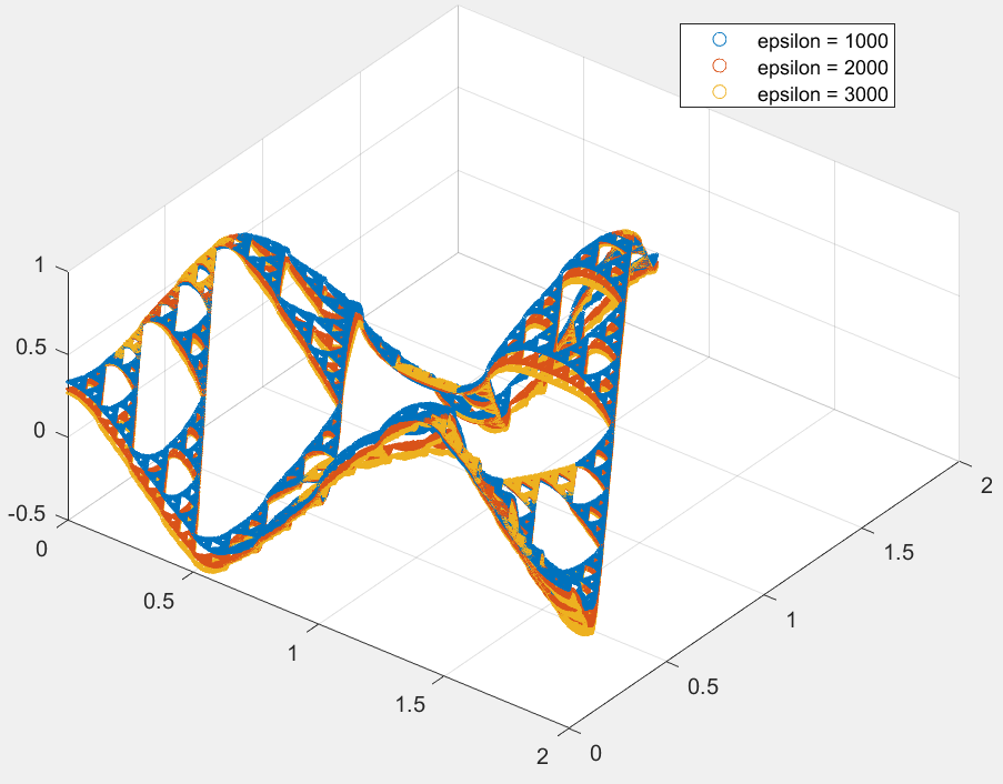
7.2. Solutions of the Mathieu Differential Equation
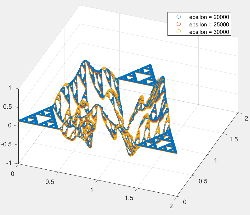
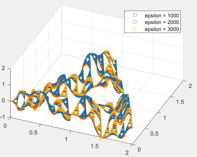
Now we investigate solutions to the fractal MDE. From Corollary 3.3 we deduce that, for a nontrivial solution (or ) to any of the four systems in section 6.2 will decay with asymptotic behavior Hence, a solution
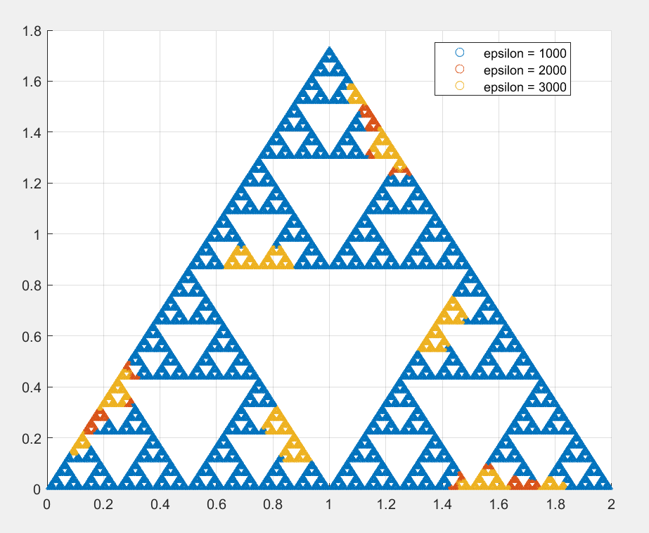
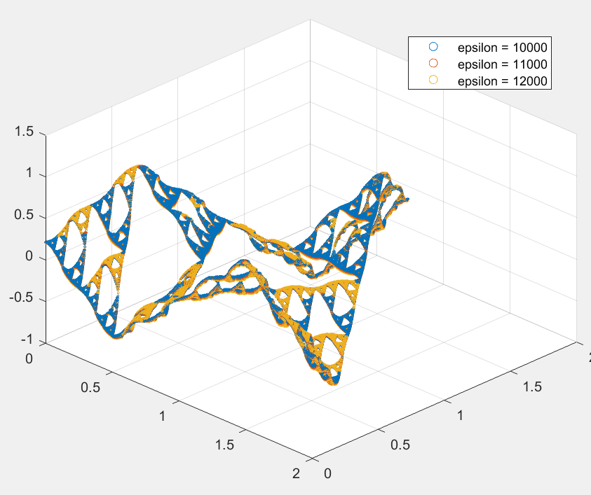
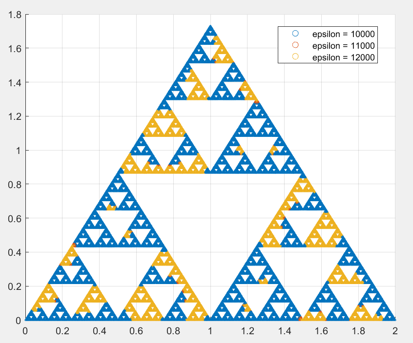
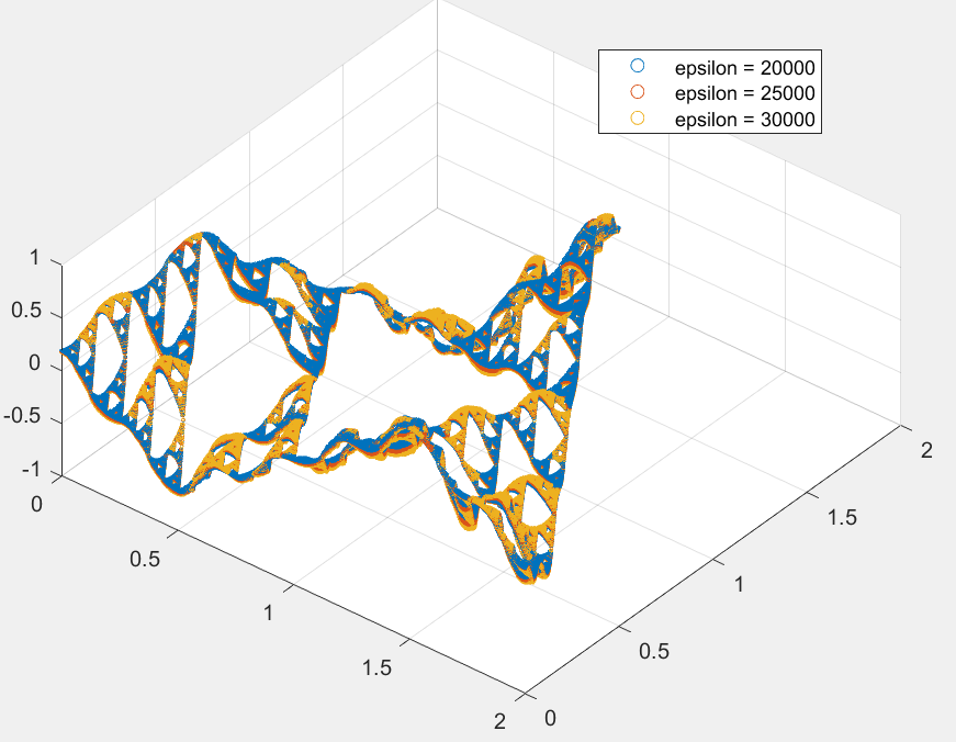
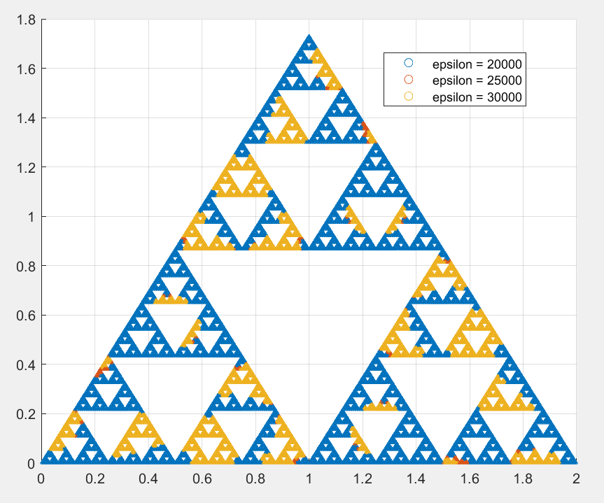
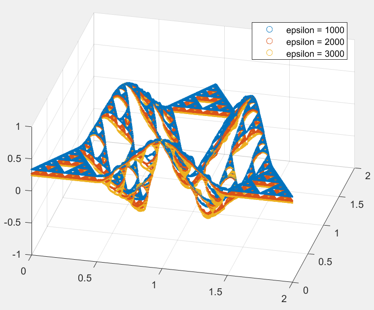
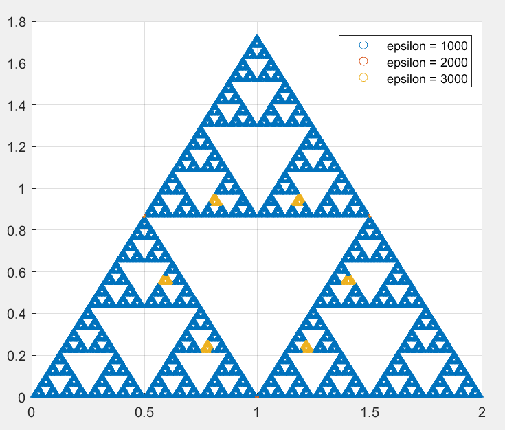
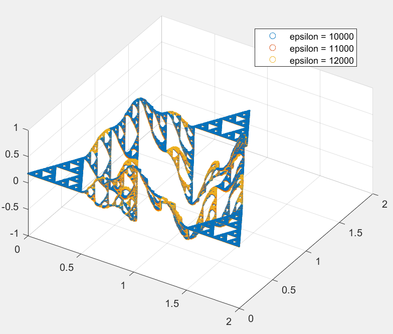
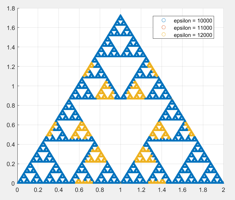
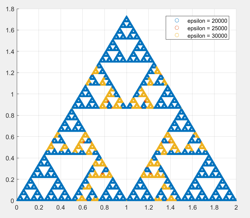
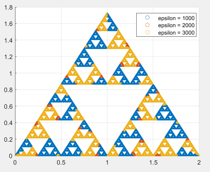
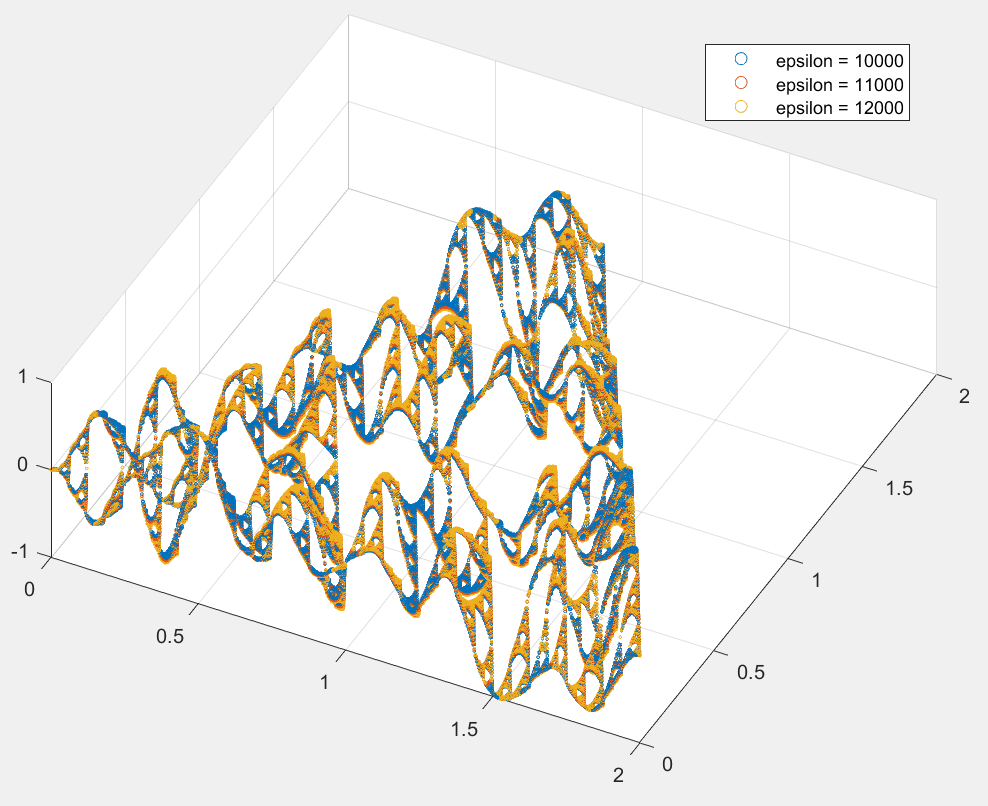
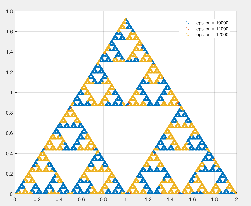
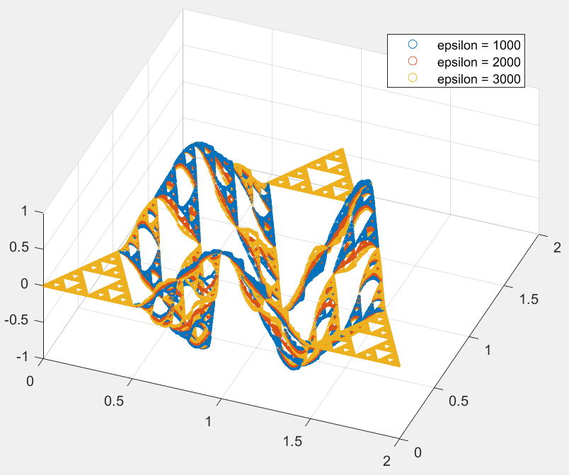
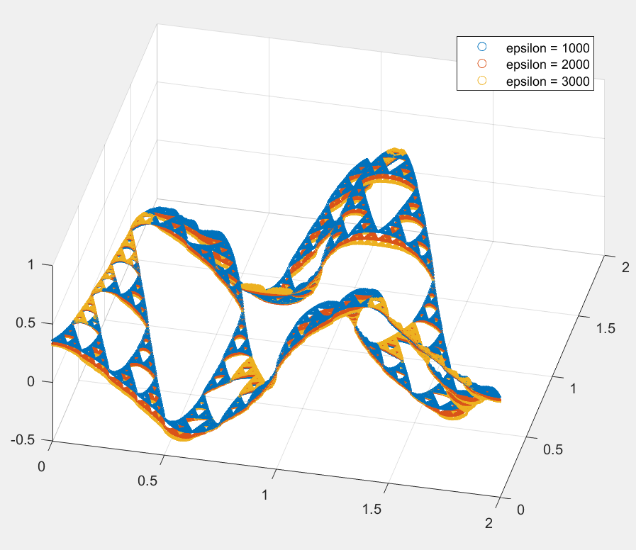
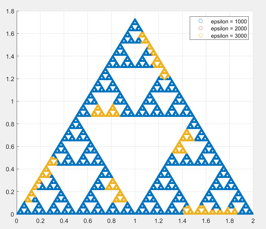
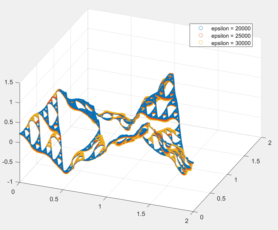
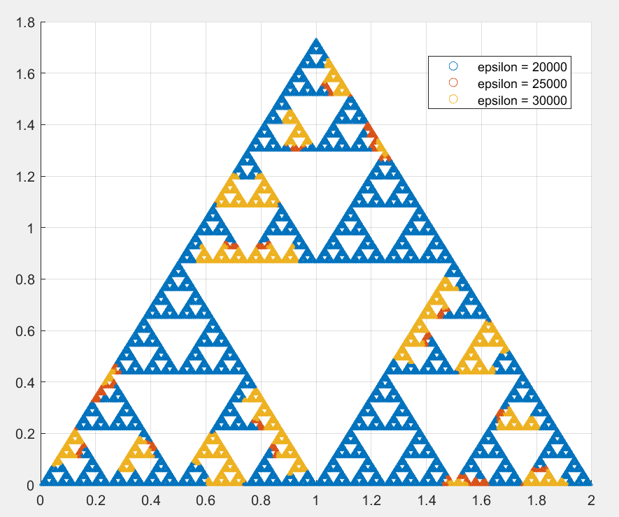
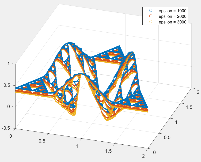
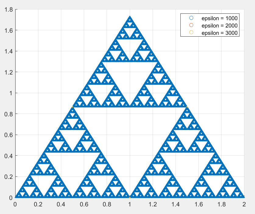
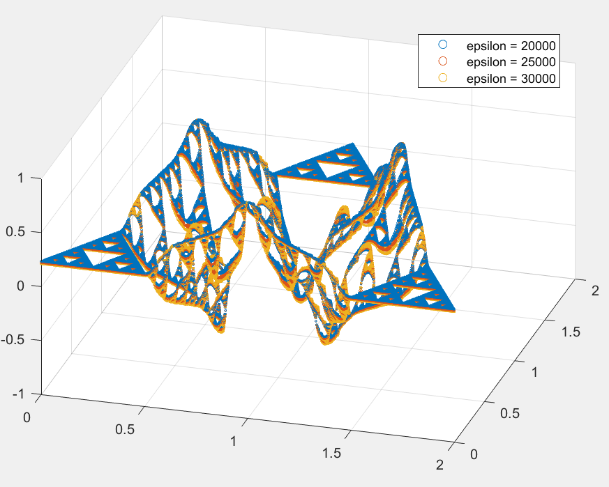
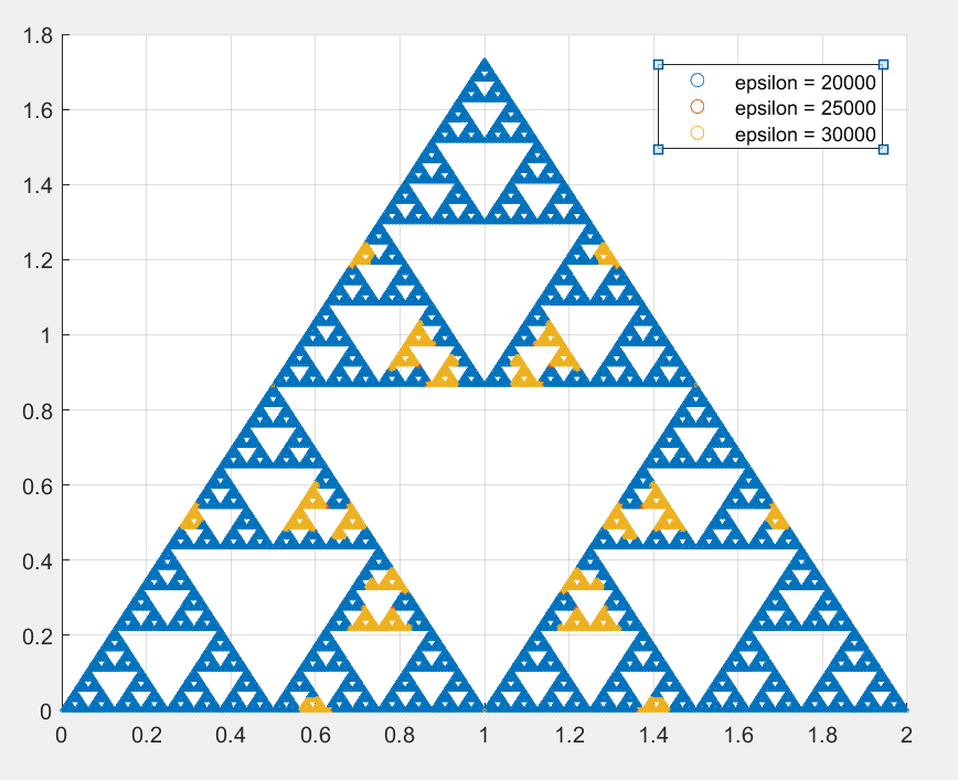
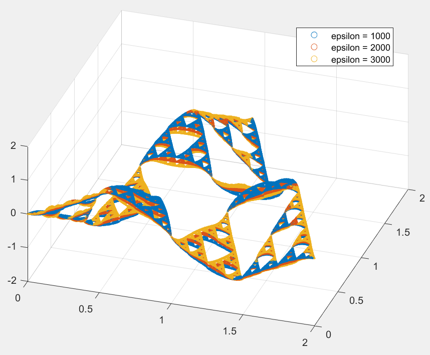
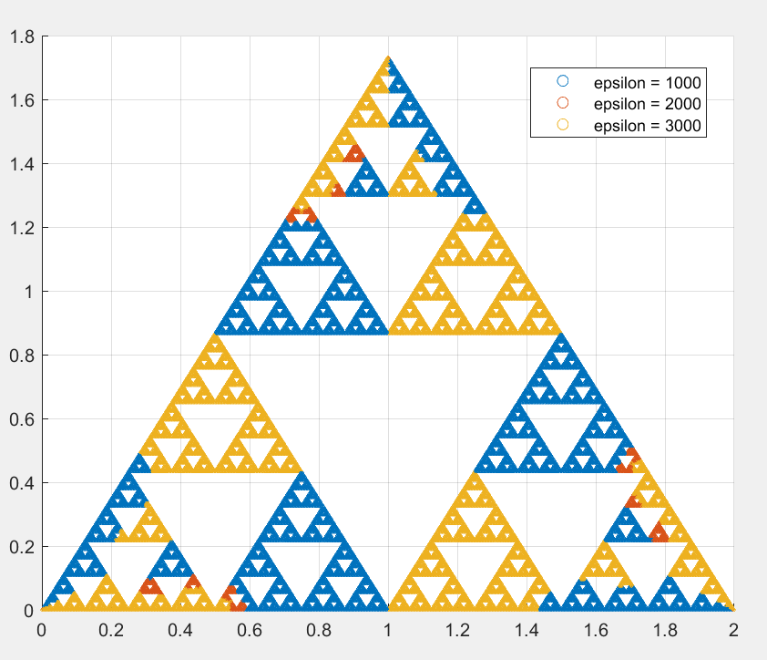
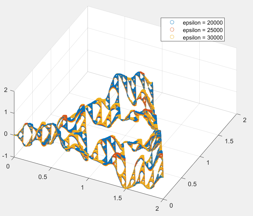
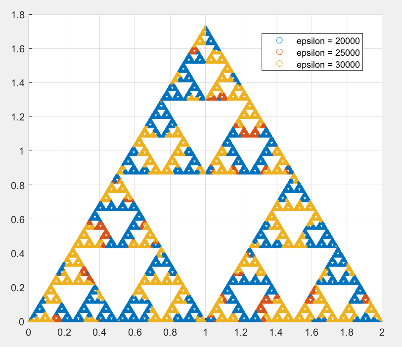
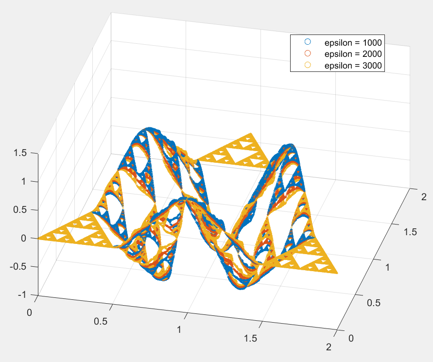
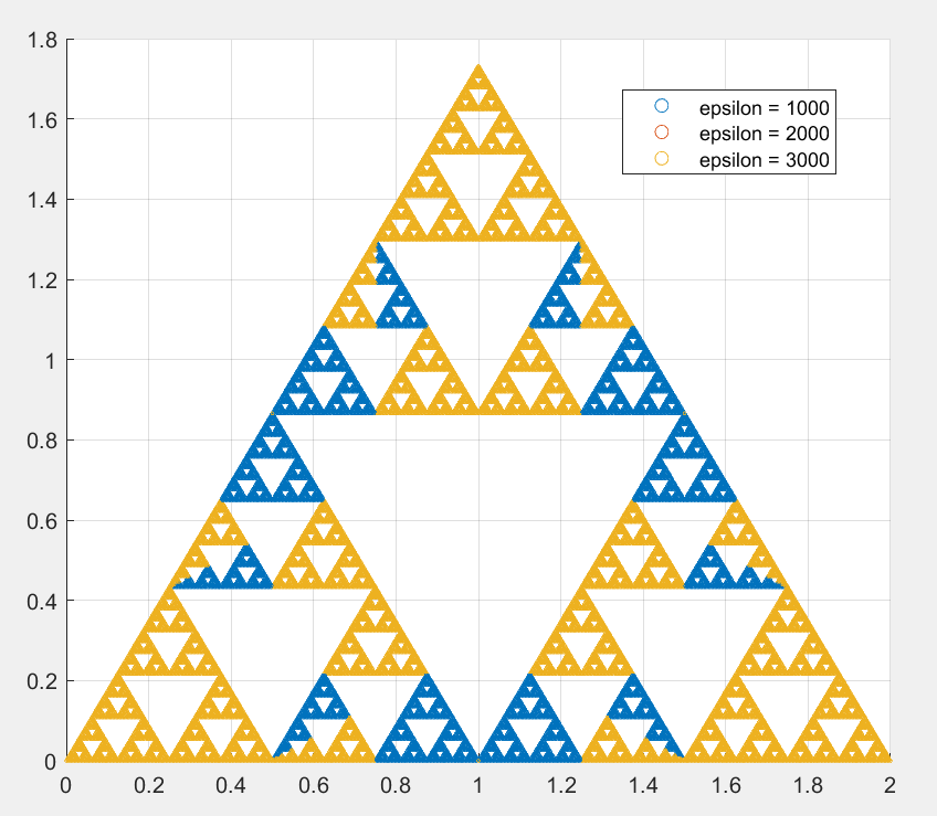
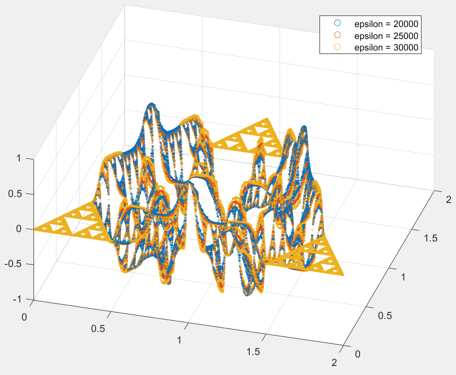
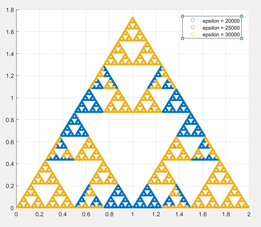
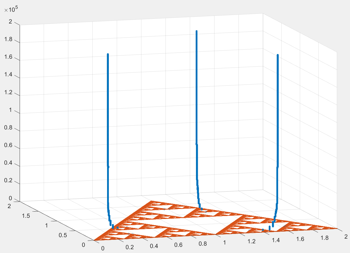
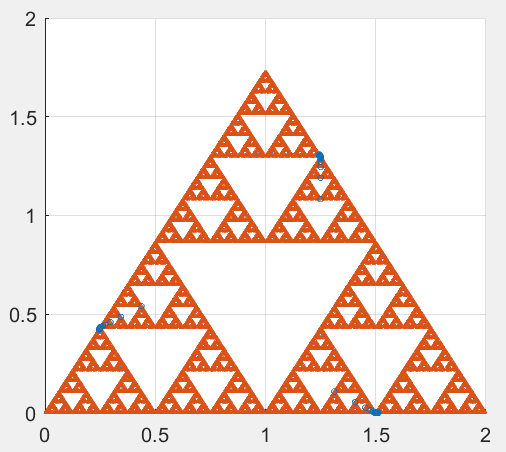
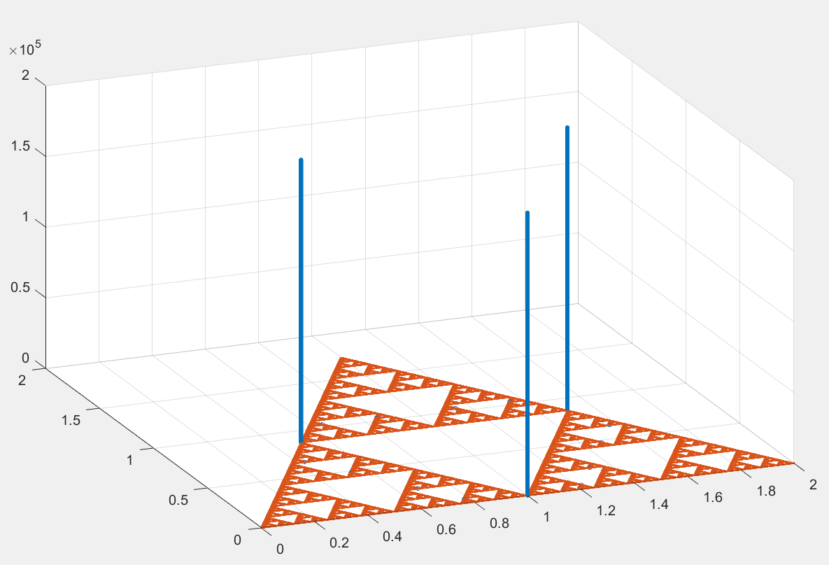
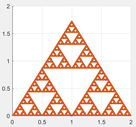
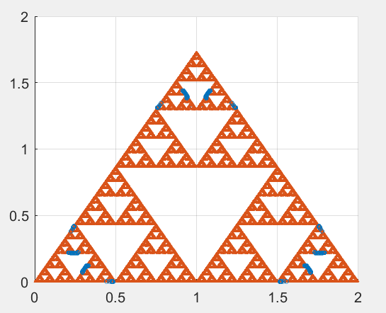
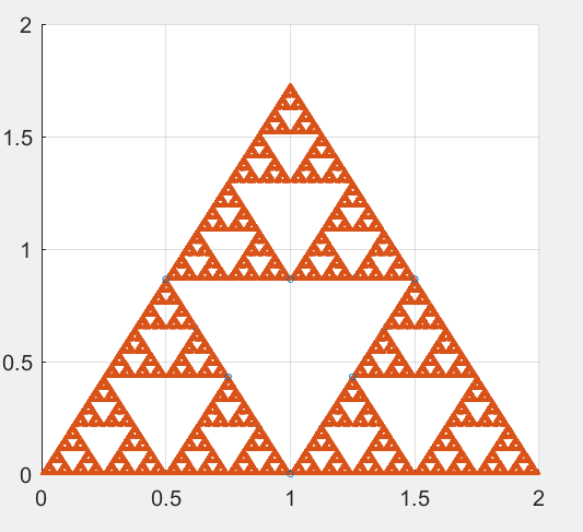
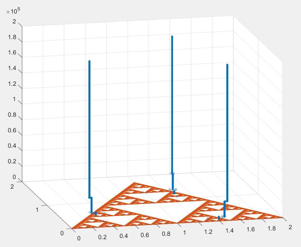
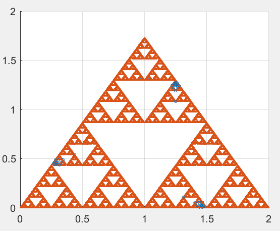
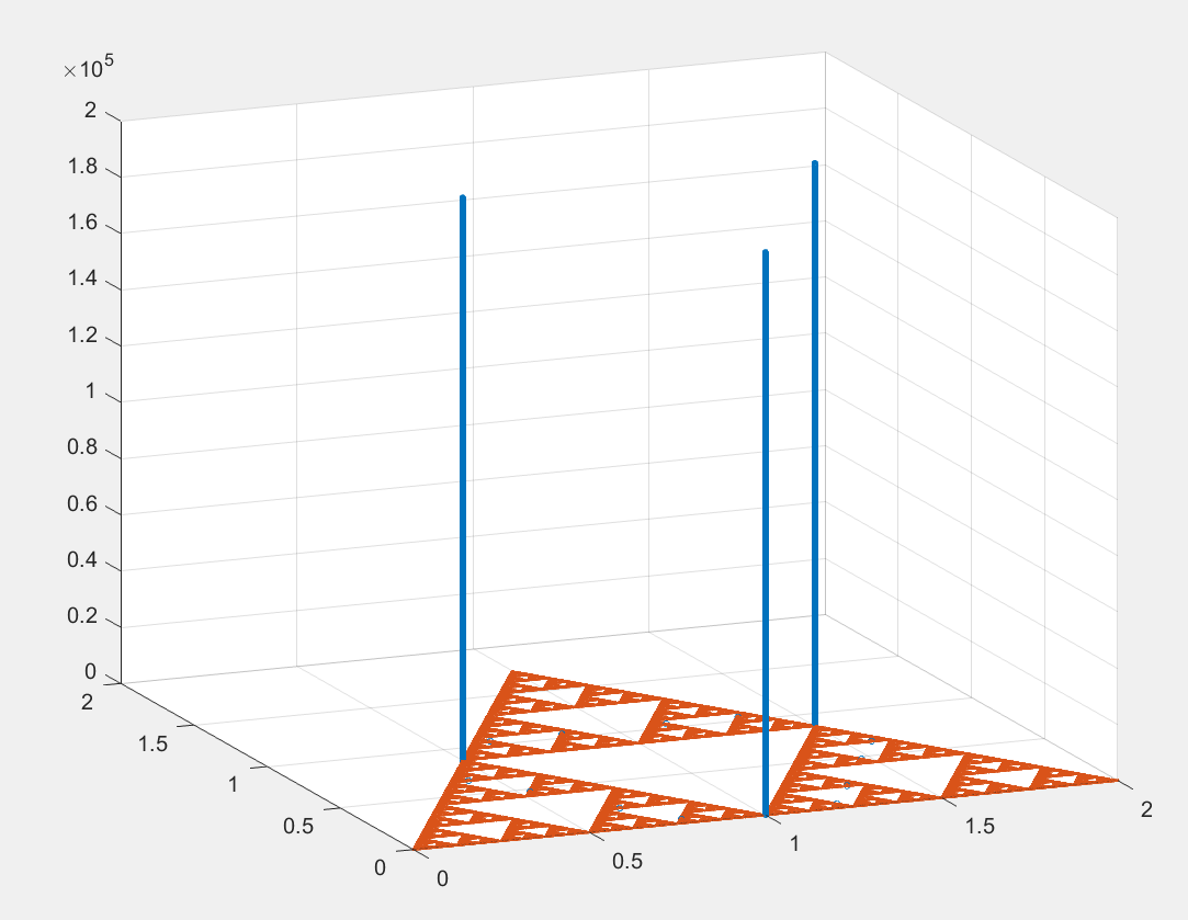
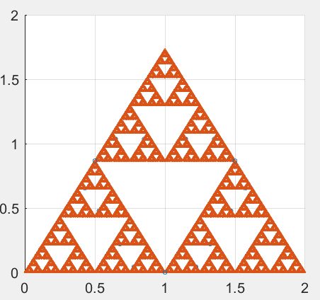
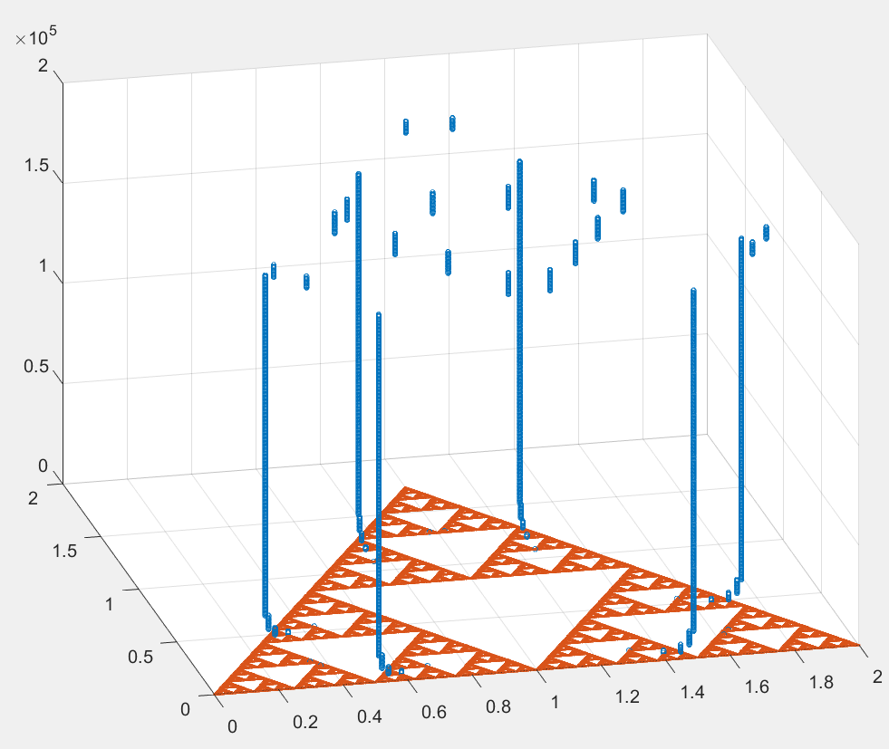
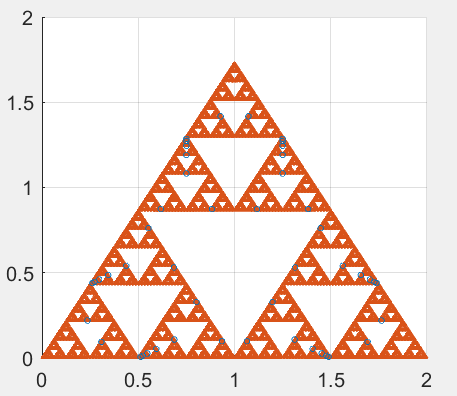
to any of the four versions of the fractal MDE may be well-approximated by the sum of just the first few terms in the series, and such an approximation will yield only a small error to the actual infinite-series solution. Recall that in Section 4 we investigated, for the MDE on the line, how properties of solutions change if one fixes a transition curve and considers periodic solutions corresponding to various points along that transition curve. We will consider the same question for the transition curves for the fractal MDE as well. We investigate this question by first studying the solutions plotted in Figures 7.10-7.29. In constructing the solutions we choose eigenfunctions of generation of birth 2 and of initial eigenvalue or , arising from either of the initial functions shown in Figure 7.9, Figures 7.10-7.15 correspond to solutions of Version 1, Figures 7.16-7.21 correspond to solutions of Version 2, Figures 7.22-7.25 correspond to solutions of Version 3, and Figures 7.26-7.29 correspond to solutions of Version 4. Each Figure includes two images. The one on the left is a plot of three different solutions corresponding to different pairs along the first transition curve; the set of three solutions in each Figure corresponds to either 5-series or 6-series, and each solution been normalized so that the maximum value it attains is 1. The image on the right in each Figure shows an overlook of the three solutions, where the color at each point indicates which solution takes on the biggest value among the three. From the plots, it is evident that these normalized solutions seem to converge as tends to infinity along the first transition curve. The second way in which we investigate the question is by observing the behavior of the location of relative maxima of solutions as traverses along a transition curve. Here we still choose to study pairs and corresponding solutions on the first transition curve for each version. See Figure 7.30-7.37. This is analogous to our study of the relative maxima of solutions to the MDE on the line in Section 4.2. Each of the Figures contains two images indicating the position of relative maxima: the image on the left shows how the positions of the maximas move as becomes larger, and the image on the right is an overlook of the left one where we can clearly see the locations of the peaks. We make several observations:
-
•
The first thing we can see is that the movement of the peaks are not large, and we do not observe the peaks converging to the boundary.
-
•
The second observation is that the and series behave quite differently. We can observe jumps of peaks in all the versions for series, but the number of peaks is usually 3. A special case is figure 7.36, where many peaks occur when is quite large. However, for series, we can observe many more peaks when is very small, but most of them do not appear when is large. Until now, we do not have explanation for these behaviors.


-
-
8. Further Research
Now we discuss further research questions that can be investigated in this area.
-
(i)
Asymptotic behavior of transition curves One could further investigate the asymptotic behavior of the transition curves. For the line case, we have Theorem 4.2 due to W.S. Loud, stating that
as on the th transition curve. We can investigate whether estimates of a similar form hold on . This would include extending Proposition 7.1 to Version 3 and Version 4 the MDE on .
-
(ii)
Other modifications of MDE matrix Further research could investigate different matrix versions of the fractal MDE, aside from Versions 1-4 presented in Section 6.
-
(iii)
Other Fractal Domains One could investigate how the Mathieu differential equation could be extended to other infinite fractafolds. Such infinite fractafolds may or may not be based on .
-
(iv)
The Hill Equation The Mathieu differential equation is actually a special case of the so-called Hill differential equation. The Hill differential equation is given by
where is an arbitrary periodic function. Readers can read [21, 16, 17, 28] for details. Further research could investigate ways in which to extend, for various choices of , the Hill differential equation to be defined on fractal domains.
9. Appendix
In this appendix we derive equations in matrix form for solutions to the MDE on the line which have period , . We will use a similar procedure as in Section 2 and will obtain tridiagonal matrices. Let be a solution with period . We can write the Fourier expansion of as
| (9.1) |
Plugging in this Fourier series for into the Mathieu differential equation, we obtain two infinite systems of linear homogeneous equations for the cosine and sine coefficients, respectively, as follows:
and
We can immediately write the equations in the matrix form, but the result is unwieldy. So, we make further classifications of the coefficients, just as we did in Section 2.2, where coefficients are separated into two classes—those with even indices and those with and odd indexes. A natural criterion is to have coefficients that appear in the same equation be in a same class. For example, and should be in a same class. Based on this idea, we say that and (or and ) are in the ‘same class’ if and only if there is a finite sequence
such that and appear in a same equation for all . For example, and are in the same class, since we and are in the same equation, and are in the same equation, and and are in the same equation. It is easy to check that the the property of being in the ‘same class’ is an equivalence relation on the set and on the set . This partitions into different equivalence classes and partitions into different equivalence classes. So we can write equations for different equivalence classes separately. Below, we discuss all the possible cases. First we give a discussion for the cosine coefficients . As we will see, the case for the sine coefficients is similar. There are three possible forms that the matrix corresponding to any particular equivalence class can take: 1). The first possible equivalence class is , with the corresponding matrix equation
Note that this is just the equation in Section 2.2. If there is a nontrivial solution to the above equation, then the MDE has a periodic solution, since solves the MDE. 2). The second form that an equivalence class can take is
where . The corresponding equations can be written in the form
If there is a nontrivial solution to the above equation, then is a -periodic solution to the MDE, where denotes the greatest common divisor of the pair . In particular, we get a -periodic solution to the MDE from the equation above if and only if and are coprime. Thus, the matrices of the second form with and coprime yield -periodic solutions. 3) The third form that an equivalence class can take is This form can only occur if is even. The corresponding equations can be written in the form
The above matrix is exactly the matrix in Section 2.2, which yield -periodic solutions.
The matrix forms for sine coefficients are quite similar to those for the cosine coefficients. For solutions of period , the equations for sine coefficents have the following form
where can by any integer such that and are coprime.
Acknowledgements
This research was hosted by the Cornell University Department of Mathematics through its 2018 Summer Program for Undergraduate Research. Anthony Coniglio’s participation in this research was partly supported by Indiana University Bloomington. Xueyan Niu’s participation in this research was partly supported by the Overseas Research Fellowship (ORF) of Faculty of Science, University of Hong Kong.
References
- [1] N. Asai, D. Cai, Y. Ikebe and Y. Miyazaki “The Eigenvalue Problem for Infinite Complex Symmetric Tridiagonal Matrices With Application” In Linear Algebra Appl. 241, 1996, pp. 599–618
- [2] J. Avron and B. Simon “The asymptotics of the gap in the Mathieu equation” In Ann. Physics 134, 1981, pp. 76–84
- [3] O. Ben-Bassat, R.S. Strichartz and A. Teplyaev “What Is Not in the Domain of the Laplacian on Sierpinski Gasket Type Fractals” In J. Funct. Anal. 166, 1999, pp. 197–217
- [4] S. Cao, A. Coniglio, X. Niu, R. Rand and R.S. Strichartz “The Mathieu Differential Equation and Generalizations to Infinite Fractafolds”, 2019 URL: http://pi.math.cornell.edu/~aac254
- [5] K. Dalrymple, R.S. Strichartz and J.P. Vinson “Fratal Differential Equations on the Sierpinski Gasket” In J. Fourier Anal. Appl. 5, 1999, pp. 203–284
- [6] S. Du, Y. Jia and A.. Seshia “Twenty-Eight Orders of Parametric Resonance in a Microelectromechanical Device for Multi-band Vibration Energy Harvesting” In Sci. Rep. 6, 2016, pp. 30167
- [7] K. Falconer “Fractal Geometry” John Wiley & Sons, 2014
- [8] M. Fukushima and T. Shima “On a spectral analysis for the Sierpinski gasket” In Potential Anal. 1, 1992, pp. 1–35
- [9] A. Gil, S. Javier and N.. Temme “Numerical methods for special functions.” Society for IndustrialApplied Mathematics, 2007
- [10] H. Hochstadt “On the Width of the Instability Intervals of the Mathieu Equation” In SIAM J. Math. Anal. 15.1, 1984, pp. 105–107
- [11] J.E. Hutchinson “Fractals and self-similarity” In Indiana Univ. Math. J. 30, 1981, pp. 713–747
- [12] M. Ionescu, L.G. Rogers and R.S. Strichartz “Pseudo-differential operators on fractals and other metric measure spaces” In Rev. Mat. Iberoam. 29, 2013, pp. 1159–1190
- [13] J. Kigami “A harmonic calculus on the Sierpiński spaces” In Japan J. Appl. Math. 6.2, 1989, pp. 259–290
- [14] J. Kigami “Analysis on fractals” 143, Cambridge Tracts in Mathematics Cambridge University Press, Cambridge, 2001
- [15] J. Kigami “Harmonic calculus on p.c.f. self-similar sets” In Trans. Amer. Math. Soc. 335.2, 1993, pp. 721–755
- [16] D.. Levy and J.. Keller “Instability Intervals of Hill’s Equation” In Comm. Pure Appl. Math. 16.4, 1963, pp. 469–476
- [17] W.. Loud “Stability regions for Hill’s equation” In J. Differential Equations 19 Elsevier, 1975, pp. 226–241
- [18] R.. Rand “Mathieu’s Equation” International Centre for Mechanical Sciences, 2016
- [19] R.H. Rand “Computer Algebra in Applied Mathematics: An Introduction to MACSYMA” Pitman Advanced Publishing Program, 1984
- [20] H. Ruan and R.S. Strichartz “Covering maps and periodic functions on higher dimensional Sierpinski gaskets” In Canad. J. Math. 61.5, 2009, pp. 1151–1181
- [21] J.. Stoker “Nonlinear vibrations in mechanical and electrical systems” New York: Interscience Publishers, 1950
- [22] R.S. Strichartz “Differential Equations on Fractals: A Tutorial” Princeton University Press, 2006
- [23] R.S. Strichartz “Fractafolds based on the Sierpiński gasket and their spectra” In Trans. Amer. Math. Soc. 355.10, 2003, pp. 4019–4043
- [24] R.S. Strichartz “Fractals in the large” In Can. J. Math. 50, 1996, pp. 638–657
- [25] R.S. Strichartz “Periodic and almost periodic functions on infinite Sierpinski gaskets” In Canad. J. Math. 61.5, 2009, pp. 1182–1200
- [26] R.S. Strichartz and A. Teplyaev “Spectral analysis on infinite Sierpiński fractafolds” In J. Anal. Math. 116, 2012, pp. 255–297
- [27] A. Teplyaev “Spectral Analysis on Infinite Sierpiński Gaskets” In J. Funct. Anal. 159.2, 1998, pp. 537–567
- [28] M.. Weinstein and J.. Keller “Asymptotic Behavior of Stability Regions for Hill’s Equation” In J. Appl. Math. 47.5 SIAM J. Appl. Math., 1987, pp. 941–958