Asymptotic independence and support detection techniques for heavy-tailed multivariate data

Abstract

One of the central objectives of modern risk management is to find a set of risks where the probability of multiple simultaneous catastrophic events is negligible. That is, risks are taken only when their joint behavior seems sufficiently independent. This paper aims to help to identify asymptotically independent risks by providing additional tools for describing dependence structures of multiple risks when the individual risks can obtain very large values.

The study is performed in the setting of multivariate regular variation. We show how asymptotic independence is connected to properties of the support of the angular measure and present an asymptotically consistent estimator of the support. The estimator generalizes to any dimension $N\geq 2$ and requires no prior knowledge of the support. The validity of the support estimate can be rigorously tested under mild assumptions by an asymptotically normal test statistic.

2010 MSC: Primary 62E20 60G70, Secondary 62G05 60G57

1 Introduction

This paper contributes partial solutions to two problems: How can one decide if random variables are asymptotically independent and how can their dependence structure be visualized, quantified and analyzed in practice? Our approach uses exploratory methods where grid based support estimates generate hypotheses about dependence. These exploratory methods are combined with a testing scheme relying on asymptotic normality.

Both finance and insurance benefit from having robust tools for understanding extremal dependence; that is, the dependence of extreme values such as losses or claims. In finance, one of the central tasks of risk management is to classify assets into classes that have minimal or no extremal dependence. The joint behavior of individual assets affects portfolio allocation strategies and ultimately determines which equities are selected for a portfolio. By selecting equities for the portfolio that are as independent as possible, we reduce portfolio risk since the portfolio is unlikely to experience many large losses at once. Our method can be viewed as a way to reduce the amount of systemic risk of a portfolio. In insurance, large claims are a major risk factor because they can cause insolvency. This risk is more serious if multiple lines of business can suffer large claims at the same time. Furthermore, successful pricing of insurance contracts as well as negotiations with reinsurance providers depend on having an understanding of the worst case risks. Thus, it is necessary to have an accurate dependence model especially for large claims.

We assume that all of the multivariate risks are heavy-tailed which for this paper means the distributions of risk vectors are multivariate regularly varying (MRV) [49]; this is defined in Section 1.4. In heavy tailed modeling, there are many complementary studies recommending methods for quantifying or modeling multivariate extremal dependence. Copula methods [32, 30, 31, 25, 23, 40, 45] have a large literature and are not restricted to heavy tails. Extreme value methods focus on quantifying asymptotic dependence between pairs using numerical summaries such as the coefficient of tail dependence ([7, p. 163], [15, p258], [46, 24, 8]) or similar concepts like the extremal dependence measure [35, 48] or the extremogram[39, 13, 14]. Other studies concentrate on estimating the limit measure of regular variation or the angular measure [20, 19, 18, 16, 49] and additionally there is the hidden regular variation stream of inquiry about whether multiple distinct heavy tail asymptotic regimes coexist [42, 43, 11, 10, 12, 49, 28, 37, 47]. There are recent efforts to assess dependence by estimating the support of the limit measure of regular variation [12, 51, 27] and growing interest in issues around dimension reduction of high-dimensional heavy tailed vectors [27, 50, 8, 21, 29]. Beyond the MRV setting, similar topics have been discussed from the extreme value theoretical viewpoint; see e.g. [22, Section  6] and its references.

Our approach relies on an exploratory step in which we assess dependence by estimating the support of the limit measure. The support of the limit measure can indicate if the risk vector components are strongly asymptotically dependent or asymptotically independent. This step is used to generate hypotheses about the dependence structure which can then be tested more formally using test statistics that are asymptotically normal. Support estimation is accomplished using what we call the grid based estimator which first bins the data and then counts bin frequencies. We use this binning method to speed computation anticipating cases where dimensions and sample sizes are large enough to cause computing problems.

Assuming the data follows a standard multivariate regularly varying distribution, the data is first thresholded based on the magnitudes of sample vectors and then divided into two parts. The first part is used to establish the grid based estimation of the support of the limit measure and to generate hypotheses about the dependence structure. The remaining data is used to test the validity of the support estimate using an asymptotically normal test statistic.

1.1 Why conventional risk measures relying on correlation may mislead.

In applications centered on extreme risk, conventional moment based risk measures such as correlation are potentially misleading. This is a persistent message in the extreme value and heavy tails literature. Typically, the dependence structure of large observations determines worst case risk and small observations may have minimal impact on worst case risk even if highly dependent. The following toy example illustrates inadequacies of correlation.

Example 1.1.

Let $\alpha>2$ and $l>1$. Suppose $X,Z$ and $B$ are independent random variables such that $\mathbb{P}(X>x)=\mathbb{P}(Z>x)=x^{-\alpha}$ for $x\geq 1$ and $1$ otherwise. Let $\mathbb{P}(B=0)=1-\mathbb{P}(B=1)=1/2$. Set

$$Y_{1}:=X\mathbbm{1}(X\leq l)+lZB\mathbbm{1}(X>l)$$

and

$$Y_{2}:=Z\mathbbm{1}(X\leq l,Z\leq l)+X\mathbbm{1}(X>l).$$

Suppose the pairs $(X,Z)$ and $(X,Y_{i})$, $i=1,2$, denote risks to a company where the components of vectors correspond to different lines of businesses. The aim of the company is to avoid insolvency from large losses, so the pair $(X,Y_{1})$ should not be considered more risky than $(X,Z)$ because the probability of two simultaneous catastrophic losses exceeding $x>l$ for both vectors is of order $x^{-2\alpha}$ . On the other hand, the pair $(X,Y_{2})$ is riskier than $(X,Y_{1})$ or $(X,Z)$, because $Y_{2}=X$ when $X>l$, resulting in the probability of two catastrophic losses exceeding $x>l$ to be of order $x^{-\alpha}$.

However, one reaches contradictory conclusions if correlation is used to quantify riskiness. Due to independence of $X$ and $Z$, $\textnormal{Corr}(X,Z)=0$. However, $\textnormal{Corr}(X,Y_{1})\to 1,$ as $l\to\infty$. In addition, the pair $(X,Y_{2})$ is asymptotically fully dependent for all $l>1$ using the terminology of [12] since $P[X>x,Y_{2}>x]\sim x^{-\alpha}$. Yet, $\textnormal{Corr}(X,Y_{2})\to 0,$ as $l\to\infty$. So, using correlation as a measure of risk in this example leads to overestimation of insignificant risk for $(X,Y_{1})$ as well as underestimation of potentially catastrophic risk for $(X,Y_{2})$.

Correlation, along with other popular risk metrics, fails to adequately quantify risk in Example 1.1 because it has limited capability of describing dependence of rare events. Similar phenomena as in Example 1.1 have been observed in nature. In [50], the authors study meteorological data in order to model extreme ground level ozone events. The study depicts cases where the etremal observations have significantly different dependence structure than small observations, see e.g. Figure 1 of [50].

In conclusion, modeling dependence structures with emphasis on accuracy of tail behavior requires different tools than modeling systems as a whole. When the MRV or extreme value framework is applicable, the methods presented in Sections 2 and 3 overcome some of the shortcomings of previous approaches and allow practitioners to more fully understand how each risk contributes to overal risk management goals in finance and insurance.

1.2 Structure of the paper

The rest of Section 1 defines notation, concepts and definitions. In Section 2, the grid based asymptotic support estimator for multivariate heavy-tailed data is presented. Consistency and related properties are proved in Sections 2.2 and 2.3. We review the definition of asymptotic independence as well as connections with limiting behavior of heavy tailed random vectors in Section 3 and we introduce a test for asymptotic independence based on asymptotic normality in Section 3.3. We illustrate the techniques developed in Sections 2 and 3 by means of simulated and real examples in Section 4.

1.3 Basic definitions

Suppose $(\Omega,\mathcal{B},\mathbb{P})$ is a probability space where all the subsequent random variables are defined. Throughout the paper random variables take values in a metric space $(\mathbb{R}^{N},d)$, where $N\geq 2$ is the dimension of the space, and $d=d_{\mathbb{R}^{N}}$ is the $L_{2}$ or Euclidean distance: for ${\bf x}=(x^{(1)},x^{(2)},\ldots,x^{(N)})$ and ${\bf y}=(y^{(1)},y^{(2)},\ldots,y^{(N)})$, $d({\bf x},{\bf y})=\sqrt{\sum_{i=1}^{N}(x^{(i)}-y^{(i)})^{2}}$. The $L_{2}$-distance is used in mappings that project sets into lower dimensional spaces in a way that does not distort the image. However, unless otherwise stated, $||\cdot||$ denotes the $L_{1}$-norm, where $||{\bf x}||=\sum_{i=1}^{N}|x^{(i)}|.$ The $L_{1}$-norm is often natural because in applications the total risk is typically the sum of marginal risks. So, any condition on the size of the $L_{1}$ norm can be directly viewed as a condition on the total risk.

Upper indices are used to identify components of vectors. Lower indices are reserved for order statistics. For $1\leq i\leq N$, the $i$th largest component of ${\bf x}$ is $x_{(i)}$. All inequalities and operations involving vectors are understood componentwise as in Section 1.2 of [47]. It is convenient to set $\boldsymbol{1}=(1,\dots,1)$ where the dimension is clear from context. For a finite set $A$, the number of elements in $A$ is denoted by $\#A$.

For a metric space $\mathbb{E}$, we set $M_{+}(\mathbb{E})$ to be the set of all non-negative Radon measures on $\mathbb{E}$; that is, measures that are finite on compact subsets of $\mathbb{E}$. The collections of open, closed and compact sets are denoted by $\mathcal{G}$,$\mathcal{F}$ and $\mathcal{K}$, respectively. For details about the Hausdorff metric on $\mathcal{K}$, see [38, 44]. For a set $A\subset\mathbb{R}^{N}$ the whole space can be partitioned as $\mathbb{R}^{N}=\textnormal{int}(A)\cup\textnormal{ext}(A)\cup\partial A$, the topological interior, exterior and boundary of the set $A$. The diameter of $A$ is denoted by $\textnormal{diam}(A)$, the complement of $A$ by $A^{c}$ and the closure of $A$ by $\textnormal{cl}(A)$. The Euclidean ball with center ${\bf x}\in\mathbb{R}^{N}$ and radius $\delta>0$ is $B({\bf x},\delta)$. The notation $:=$ is used when the left hand side is defined by the right hand side of the equation.

1.4 Multivariate regular variation

The standard definition of multivariate regular variation is defined in [49, Theorem 6.1]. We allow possibly negative values of components.

Definition 1.1.

Suppose ${\bf Z}=(Z^{(1)},Z^{(2)},\ldots,Z^{(N)})$ is a random vector in $\mathbb{R}^{N}$. Set $\mathbb{E}:=[-\infty,\infty]^{N}\backslash\{{\bf 0}\}$. We say that ${\bf Z}$ is standard multivariate regularly varying with limit measure $\nu$ if there exists a function $b(t)\uparrow\infty$, as $t\to\infty$, such that

(1.1) $$t\mathbb{P}\left(\frac{{\bf Z}}{b(t)}\in\cdot\right)\stackrel{{\scriptstyle v}}{{\to}}\nu(\cdot)$$

in $M_{+}(\mathbb{E})$, where $\stackrel{{\scriptstyle v}}{{\to}}$ stands for vague convergence of measures.

Note that normalizing all components using the same function $b$ implies that the components must be tail equivalent, see [49, Remark 6.1.].

Multivariate regular variation has an equivalent definition via the probability measure $\mathbb{S}$, called the angular measure or spectral measure defined on the $L_{1}$-unit sphere

(1.2) $$C^{N}:=\left\{{\bf z}\in\mathbb{R}^{N}:||{\bf z}||=1\right\}.$$

Then equivalently, ${\bf Z}$ is standard multivariate regularly varying if there exist a function $b(t)\uparrow\infty$, as $t\to\infty$, such that for

$$(R,\Theta):=\left(||{\bf Z}||,\frac{{\bf Z}}{||{\bf Z}||}\right)$$

we have

(1.3) $$t\mathbb{P}\left(\left(\frac{R}{b(t)},\Theta\right)\in\cdot\right)\stackrel{{\scriptstyle v}}{{\to}}c\nu_{\alpha}\times\mathbb{S}$$

in $M_{+}((0,\infty]\times C^{N})$, as $t\to\infty$, where $c>0$, $\mathbb{S}$ is a probability measure on $C^{N}$ and $\nu_{\alpha}((x,\infty])=x^{-\alpha}$. The number $\alpha>0$ is called the tail index of the multivariate regularly varying distribution.

In addition to the $N$-simplex in $L_{1}$, set

$$C^{N}_{+}:=C^{N}\cap\mathbb{R}^{N}_{+}=\left\{{\bf z}\in\mathbb{R}^{N}_{+}:z^{(1)}+z^{(2)}+\cdots+z^{(N)}=1\right\}$$

to denote the part of simplex $C^{N}$ where all coordinates are non-negative. The face of the simplex corresponding to indices $A\subset\{1,2,\ldots,N\}$ is

(1.4) $$C^{N}(A):=\left\{{\bf z}\in C^{N}:z^{(i)}=0,\textnormal{ when }i\notin A\right\}.$$

1.5 The support of a measure

The asymptotic dependence structure of ${\bf Z}$ is controlled by the angular measure $\mathbb{S}(\cdot)$ and considerable information about extremal dependence is contained in the support.

Definition 1.2 (Support of measure in $\mathbb{R}^{N}$).

If $\mu$ is a measure on $\mathbb{R}^{N}$, the support $\textnormal{\bf{supp}}(\mu)$ of $\mu$ is the set

$$\textnormal{\bf{supp}}(\mu):=\left\{{\bf z}\in\mathbb{R}^{N}:\mu(B({\bf z},\delta))>0\textnormal{ for all }\delta>0\right\}.$$

Also, $\textnormal{\bf{supp}}(\mu)$ is the smallest closed set carrying the mass of $\mu$,

$$\textnormal{\bf{supp}}(\mu)=\bigcap_{A\in\mathcal{F},\,\mu(A^{c})=0}A.$$

The support of a measure on a suitable subset of $\mathbb{R}^{N}$ is defined similarly. We will be interested in the support supp of $\mathbb{S}$ and the part of the support of $\mathbb{S}$ on simplex $C_{+}^{N}$ is denoted by $\textnormal{\bf{supp}}^{+}$.

1.6 $N$-simplex and simplex mappings

Section 2 estimates the support of the angular measure $\mathbb{S}$ by approximating the support of $\mathbb{S}$ on the positive $N$-dimensional $L_{1}$ sphere $C^{N}_{+}$. The set $C^{N}_{+}$ is first projected to an $N-1$ dimensional space $[0,1]^{N-1}$ using a bijective simplex mapping defined below. This enables us to partition the $N-1$ dimensional image space into a grid consisting of equally sized rectangles. The preimages in $C_{+}^{N}$ of the rectangles in the $N-1$ dimensional space partition the $N$ dimensional set $C^{N}_{+}$. So the use of a simplex mapping provides a simple way to partition the positive $L_{1}$ simplex and offers improved visualization. In particular, when $N=3$, the visual representation of the support estimate is a planar set.

Rectangles accepted into the estimated support are determined from the data by the concentrations of probability mass of the empirical estimate of the limiting measure $\mathbb{S}$. This contrasts with [12] which assumed the support was a connected interval and estimated this interval using the range of the thresholded data. Advantages of this current approach are computational efficiency and that finding the sets of highest concentration provides a way to eliminate noise arising from unlikely observations that lie outside of the asymptotic support.

Definition 1.3.

Let $N\geq 2$. Suppose $T$ is a bijective mapping $T\colon C_{+}^{N}\to[0,1]^{N-1}$ with property

$$d_{\mathbb{R}^{N}}({\bf x},{\bf y})=ad_{\mathbb{R}^{N-1}}(T({\bf x}),T({\bf y}))$$

for all ${\bf x},{\bf y}\in C_{+}^{N}$ and some constant $a>0$. Such a mapping $T$ is called a simplex mapping associated with $C_{+}^{N}$.

When $N=3$ a simplex map aids visualization because supports can be visualized in $\mathbb{R}^{2}$. There is flexibility when choosing the mapping $T$ so the grid positioning can be adjusted with respect to observed data if necessary. By shifting the grid, one can avoid concentration of points on grid boundaries.

Example 1.2.

1. If $N=2$, one can set

   $$T\left(\begin{bmatrix}z_{1}\\ z_{2}\\ \end{bmatrix}\right)=z_{1}.$$

   Here, $a=\sqrt{2}$.

2. If $N=3$, setting

   $$T\left(\begin{bmatrix}z_{1}\\ z_{2}\\ z_{3}\\ \end{bmatrix}\right)=\begin{bmatrix}\frac{1}{2}(z_{2}-z_{1}+1)\\ \frac{\sqrt{3}}{2}z_{3}\\ \end{bmatrix}$$

   gives a mapping $C_{+}^{3}\mapsto[0,1]^{2}$. The image $T(C_{+}^{3})$ is a region in $[0,1]^{2}$ inside an equilateral triangle with edges on $(0,0),(1,0)$ and $(1/2,\sqrt{3}/{2})$. The isometry property in Definition 1.3 can be shown to hold by observing that $z_{3}=1-z_{2}-z_{1}$ and writing the expressions for the squared $L_{2}$ distances in $\mathbb{R}^{3}$ and $\mathbb{R}^{2}$. The property holds with $a=\sqrt{2}$. Mapping T has an inverse $T^{-1}\colon T(C_{+}^{3})\to C_{+}^{3}$ given by

   $$T^{-1}\left(\begin{bmatrix}z_{1}\\ z_{2}\\ \end{bmatrix}\right)=\begin{bmatrix}1-z_{1}-\frac{z_{2}}{\sqrt{3}}\\ z_{1}-\frac{z_{2}}{\sqrt{3}}\\ \frac{2z_{2}}{\sqrt{3}}\\ \end{bmatrix}.$$

The mapping of Example 1.2 is used to visualize 3-dimensional data in 2-dimensions in Section 4.

2 Support estimation

This section defines the grid based estimator and shows asymptotic consistency under general assumptions. Suppose $N\geq 2$ is the dimension of the data and $m\geq 2$ is an integer that determines the resolution of the asymptotic support estimate. We map the $N$-dimensional simplex into $[0,1]^{N-1}$ and then the image is partitioned into $m^{N-1}$ smaller sets. The partition is called a grid and the sub-squares (or cubes in higher dimensions) are cells. Some grid cells are accepted as part of the support while the rest are rejected based on a data driven rule described in Section 2.

The topic of support estimation has antecedents though not usually in the context of estimating the support of an asymptotic distribution. See [2, 41, 5, 1, 34, 26, 9]. A support estimation problem in [4] assumes a uniform distribution over a convex set. Estimating the support from a sample by placing a small ball around each sample point was suggested in [17] and followed up in [3]; this method has some overlap with our proposal. The method in [10, Proposition 6.3] for estimating an asymptotic support omits a condition.

2.1 Support estimator and related quantities

2.1.1 Reduction to positive quadrant.

Random vectors in $\mathbb{R}^{N}$ can be considered to have $2N$ tails but usually without loss of generality it is enough to write proofs for the positive quadrant since negative components can be reflected into positive values by multiplying by $-1$. Let ${\bf s}\in\{-1,1\}^{N}$ be a vector of plus or minus $1$’s and for ${\bf z}\in\mathbb{R}^{N}$ define

$${\bf s}\cdot{\bf z}=(s^{(1)}z^{(1)},\dots,s^{(N)}z^{(N)}).$$

If ${\bf Z}$ is a multivariate regularly varying random vector in $\mathbb{R}^{N}$, extreme behavior of ${\bf Z}$ in a quadrant other than $\mathbb{R}_{+}^{N}$ can be studied by reducing to the case of the positive quadrant by multiplying by an appropriate ${\bf s}$. For simplicity, we present the theory, for the case where the entire support $\bf{supp}(\mathbb{S})$ is in $C^{N}_{+}$. The general case is readily reduced to this one.

For a simplex mapping $T$ and a multivariate regularly varying random vector ${\bf Z}\in{\mathbb{R}^{N}_{+}}$, define the $N-1$ dimensional random variable ${\bf U}$ as

(2.1) $${\bf U}:=T({{\bf Z}}/{||{\bf Z}||}).$$

2.1.2 Partition $[0,1]^{N-1}$ into cells.

Given a vector ${\bf x}\in[0,1]^{N-1}$ and $m\geq 2$, define a cell $\textnormal{M}({\bf x},m)\subset\mathbb{R}^{N-1}$ by

(2.2) $$\textnormal{M}({\bf x},m):= {\bf x}+\left[0,1/m\right)^{N-1}=[{\bf x},{\bf x}+\frac{1}{m}\boldsymbol{1})$$

$$= \Big{[}x^{(1)},x^{(1)}+\frac{1}{m}\Big{)}\times\cdots\times\Big{[}x^{(N-1)},x^{(N-1)}+\frac{1}{m}\Big{)}$$

which is just the box $[0,1/m)^{N-1}$ shifted by the vector ${\bf x}$. For any natural number $n$, set $[n0]=\{0,\dots,n-1\}$ and define

(2.3) $$G_{m}:= ([m0]/m)^{N-1}$$

So

$$G_{m}=\left\{{\bf x}\in[0,1]^{N-1}:x^{(i)}\in\left\{0,\frac{1}{m},\frac{2}{m},\ldots,\frac{m-1}{m}\right\},i=1,\ldots,N-1\right\}.$$

2.1.3 Approximate the support.

After partitioning the set $T(C^{N}_{+})$ by grid cells, we rasterize the asymptotic support of $\mathbb{S}_{T}=\mathbb{S}\circ T^{-1}$ for computational efficiency and then estimate this approximation to the asymptotic support. The estimation is done by mapping thresholded observations and creating cell counts.

The definitions of the rasterized support, the grid based support estimator and the proof of estimator consistency depend on Proposition 6.2 of [10, p. 158] or [49, p. 308] which give

(2.4) $$\hat{\mathbb{S}}_{n}(\cdot):=\frac{1}{k}\sum_{i=1}^{n}\mathbbm{1}(||{\bf Z}_{i}||>||{\bf Z}_{(k+1)}||)\epsilon_{{\bf Z}_{i}/||{\bf Z}_{i}||}(\cdot)\Rightarrow\mathbb{S}(\cdot),$$

as $n\to\infty$, $k=k(n)\to\infty$, $n/k\to\infty$ in $\mathbb{P}(C^{N})$, the space of probability measures on $C^{N}$ and the limit is non-random so convergence also holds in probability. This convergence is preserved under the mapping $T$ and we define

(2.5) $$\mathbb{S}_{T}=\mathbb{S}\circ T^{-1},\quad\ \hat{\mathbb{S}}_{n,T}=\hat{\mathbb{S}}_{n}\circ T^{-1}=\frac{1}{k}\sum_{i=1}^{n}\mathbbm{1}(||{\bf Z}_{i}||>||{\bf Z}_{(k+1)}||)\epsilon_{{\bf U}_{i}}.$$

Then we have

(2.6) $$\hat{\mathbb{S}}_{n,T}\Rightarrow\mathbb{S}_{T}$$

in $\mathbb{P}\bigl{(}T(C^{N})\bigr{)}$. With respect to $\mathbb{P}_{k+1}(\cdot)=\mathbb{P}(\cdot\big{|}\|{\bf Z}_{(k+1)}\|)$, the points of $\mathbb{S}_{n,T}$ are $k$ iid random elements with common distribution $\mathbb{P}({\bf U}_{1}\in\cdot\big{|}\|{\bf Z}_{1}\|>r)$ where $r$ is evaluated at $\|{\bf Z}_{(k+1)}\|.$ We denote, then

(2.7) $$\hat{\mathbb{S}}_{n,T}=\frac{1}{k}\sum_{i=1}^{k}\epsilon_{{\bf U}_{i}^{(k)}}.$$

Definition 2.1.

In the positive quadrant, ${\textnormal{\bf{Tsupp}}(m,q)}$ is the closure of

(2.8) $$\bigcup\left\{\textnormal{M}({\bf x},m):{\bf x}\in G_{m},\,\mathbb{S}_{T}(\textnormal{M}({\bf x},m))>q\right\}.$$

So, ${\textnormal{\bf{Tsupp}}(m,q)}$ is a set in $\mathbb{R}^{N-1}$. In the special case $q=0$, the set defined by ${\textnormal{\bf{Tsupp}}(m)}:={\textnormal{\bf{Tsupp}}(m,0)}$ is called the rasterised support in $\mathbb{R}^{N-1}$ and is the smallest grid set with resolution $m$ containing the support of $\mathbb{S}_{T}$.

Definition 2.2 (Support estimator).

Let ${\bf Z}_{1},{\bf Z}_{2},\ldots,{\bf Z}_{n}$ be iid multivariate regularly varying vectors in $\mathbb{R}^{N}_{+}$. Let ${\bf U}_{1},{\bf U}_{2},\ldots,{\bf U}_{n}$ be the corresponding random vectors in $\mathbb{R}^{N-1}$ obtained from transformation (2.1). Suppose $k$ and $m$ are natural numbers such that $k\geq 1$ and $m\geq 2$. For $q\in[0,1]$, the support estimator ${\widehat{\textnormal{\bf{Tsupp}}}(k,m,q)}$ of ${\textnormal{\bf{Tsupp}}(m,q)}$ is the closure of the set

(2.9) $$\bigcup\Bigl{\{}\textnormal{M}({\bf x},m):{\bf x}\in G_{m},\hat{\mathbb{S}}_{n,T}(M({\bf x},m))>q\Bigr{\}}.$$

The estimator of ${\textnormal{\bf{Tsupp}}(m)}$ is ${\widehat{\textnormal{\bf{Tsupp}}}(k,m)}$ which is ${\widehat{\textnormal{\bf{Tsupp}}}(k,m,q)}$ with $q=0$.

The support estimator ${\widehat{\textnormal{\bf{Tsupp}}}(k,m,q)}$ is a random closed set based on a random sample ${\bf Z}_{1},{\bf Z}_{2},\ldots,{\bf Z}_{n}$. It has three parameters: $k$, $m$ and $q$. Parameter $k=k(n)$ is the number of extreme observations used in estimation. For the asymptotic analysis we assume that $k=k(n)\to\infty,\;n/k(n)\to\infty$, as $n\to\infty$. Parameter $m$ denotes the resolution at which the estimate is formed. In asymptotic results, $m\to\infty$ so that the resolution grows and the cell size decreases. The parameter $q$ serves as a rejection threshold. It determines how many observations are needed in a single grid cell for the cell to be accepted as part of the support estimate. In practice it helps to reject unlikely observations and noise. If $p$ observations are required in a given sample of $n$ one can set $q=p/k(n)$.

Support estimators in Definition 2.2 are decreasing in $q$. For fixed $k,m$ and $0\leq q_{1}<q_{2}<1$,

(2.10) $${\widehat{\textnormal{\bf{Tsupp}}}(k,m,q_{2})}\subset{\widehat{\textnormal{\bf{Tsupp}}}(k,m,q_{1})}.$$

2.2 Consistency of the grid based support estimator for $q=0$

The following results are derived for the case where the limiting angular measure concentrates on the positive quadrant $C^{N}_{+}$. The general case is not mathematically much different, but requires more notation.

We begin by discussing continuity properties of the rasterization procedure.

2.2.1 The Rast operator.

The Rast operator maps sets into rasterized versions. We define for fixed resolution $m$, $\text{Rast}(\cdot,m):\mathcal{K}(T(C_{+}^{N}))\to\mathcal{K}([0,1]^{N-1})$ by

$$\text{Rast}(K,m)=\textnormal{cl}\Bigl{(}\bigcup\{M({\bf x},m):M({\bf x},m)\cap K\neq\emptyset\}\Bigr{)}.$$

So in the notation of (2.8), ${\textnormal{\bf{Tsupp}}(m)}=\text{Rast}(\text{supp}(\mathbb{S}_{T}),m).$

We begin by discussing consistency results with $m$ fixed.

Proposition 2.1.

Suppose $K$ is a compact set satisfying

(2.11) $$\forall{\bf x}\in G_{m}:\quad K\cap\textnormal{cl}(M({\bf x},m))\neq\emptyset\text{ implies }K\cap\textnormal{int}(M({\bf x},m))\neq\emptyset.$$

Then $\text{Rast}(\cdot,m)$ is continuous at $K$; that is, if $K_{n}\to K$ in the Hausdorff metric, then also $\text{Rast}(K_{n},m)\to\text{Rast}(K,m).$

Condition (2.11) says that if $K$ intersects a cell, it does not do so only on the boundary of the cell.

Proof.

We use the criterion [38, page 6] that $K_{n}\to K$ in the Hausdorff metric iff

1. (Condition 1.) $z\in K$ implies $\exists z_{n}\in K_{n}$ and $z_{n}\to z$.

2. (Condition 2.) For a subsequence $\{n_{j}\}$, if $z_{n_{j}}\in K_{n_{j}}$ and $\{z_{n_{j}}\}$ converges, then $\lim_{n_{j}\to\infty}z_{n_{j}}\in K$.

Condition 1: Assume $K_{n}\to K$ and $\boldsymbol{y}\in\text{Rast}(K,m)$. The easy case is where $\boldsymbol{y}\in K$. Then there exist $\boldsymbol{y}_{n}\in K_{n}\subset\text{Rast}(K_{n},m)$ such that $\boldsymbol{y}_{n}\to\boldsymbol{y}\in K\subset\text{Rast}(K,m)$. This verifies Condition 1 in the easy case.

Now for the more difficult case of Condition 1, assume $\boldsymbol{y}\in\text{Rast}(K,m)\setminus K$. Then there exists $\boldsymbol{x}_{0}\in G_{m}$ such that $\boldsymbol{y}\in M(\boldsymbol{x}_{0},m)$. Suppose temporarily $\boldsymbol{y}\in\textnormal{int}(M(\boldsymbol{x}_{0},m))$; this restriction will be removed. Then for some $\delta>0$, (i) $d(\boldsymbol{y},K)\geq 2\delta$; (ii) $B(\boldsymbol{y},\delta/36)\subset\textnormal{int}(M(\boldsymbol{x}_{0},m))$ (since $\boldsymbol{y}$ is in the interior of the cell); and therefore (iii) $B(\boldsymbol{y},\delta/36)\cap K=\emptyset$ (from (i)). This implies

(2.12) $$K_{n}\cap M(\boldsymbol{x}_{0},m)\neq\emptyset,\quad\text{ for all large $n$}.$$

The reason is that $M(\boldsymbol{x}_{0},m)\subset\text{Rast}(K,m)$ but $M(\boldsymbol{x}_{0},m)\cap K\neq\emptyset$ by the choice of $\boldsymbol{x}_{0}$. Condition (2.11) implies $\textnormal{int}(M(\boldsymbol{x}_{0},m))\cap K\neq\emptyset$ so $\exists\boldsymbol{y}^{*}\in\textnormal{int}(M(\boldsymbol{x}_{0},m))\cap K.$ Since $\boldsymbol{y}^{*}\in K$ and $K_{n}\to K$, $\exists\boldsymbol{y}_{n}^{*}\in K_{n}$ such that $\boldsymbol{y}_{n}^{*}\to\boldsymbol{y}^{*}$. Since $\boldsymbol{y}^{*}$ is in the interior of the cell and because $\boldsymbol{y}_{n}^{*}$ is close to $\boldsymbol{y}^{*}$, for all large $n$, $\boldsymbol{y}_{n}^{*}\in K_{n}\cap\textnormal{int}(M(\boldsymbol{x}_{0},m))$ which verifies (2.12).

Now $K_{n}$ is close to $K$ and from (2.12) has points in the cell $M(\boldsymbol{x}_{0},m)$ which miss $B(\boldsymbol{y},\delta/36)\subset M(\boldsymbol{x}_{0},m)$. Find $\boldsymbol{y}_{n}\in B(\boldsymbol{y},\delta/36)$ with $\boldsymbol{y}_{n}\to\boldsymbol{y}$. This means $\boldsymbol{y}_{n}\in\text{Rast}(K_{n},m)\setminus K_{n}\subset\text{Rast}(K_{n},m)$ and $\boldsymbol{y}_{n}\to\boldsymbol{y}\in\text{Rast}(K,m)$ as required.

If $\boldsymbol{y}\in\partial M(\boldsymbol{x}_{0},m)$ approximate $\boldsymbol{y}$ by something in the interior and proceed as above.

Condition 2: Given $\boldsymbol{y}_{n_{j}}\in\text{Rast}(K_{n_{j}},m)$ with $\boldsymbol{y}_{n_{j}}\to\boldsymbol{y}_{\infty}$ and we must show $\boldsymbol{y}_{\infty}\in\text{Rast}(K,m).$ This means we must find $\boldsymbol{x}_{0}\in G_{m}$ such that $\boldsymbol{y}_{\infty}\in M(\boldsymbol{x}_{0},m)$ and $M(\boldsymbol{x}_{0},m)\cap K\neq\emptyset.$ Because cells cover the space and there are a finite number of cells, there is a cell hit by the elements $\boldsymbol{y}_{n_{j}}$ infinitely often. Identify this cell as $M(\boldsymbol{x}_{0},m)$. So for this cell and a further subsequence $\{n_{j^{\prime}}\}\subset\{n_{j}\}$, $\boldsymbol{y}_{n_{j^{\prime}}}\in M(\boldsymbol{x}_{0},m)\subset\text{Rast}(K_{n_{j^{\prime}}},m)$ and therefore $\boldsymbol{y}_{\infty}\in\textnormal{cl}(M(\boldsymbol{x}_{0},m)).$

To verify $M(\boldsymbol{x}_{0},m)\subset\text{Rast}(K,m)$ as required do the following: Since $\boldsymbol{y}_{n_{j^{\prime}}}\in\text{Rast}(K_{n_{j^{\prime}}},m)$, there exists $\boldsymbol{y}^{*}_{n_{j^{\prime}}}\in M(\boldsymbol{x}_{0},m)\cap K_{n_{j^{\prime}}}$ and by compactness a further subsequence converges $\boldsymbol{y}^{*}_{n_{j^{\prime\prime}}}\to\boldsymbol{y}_{\infty}^{*}$ and $\boldsymbol{y}_{\infty}^{*}\in\textnormal{cl}(M(\boldsymbol{x}_{0},m))\cap K$ since $\boldsymbol{y}^{*}_{n_{j^{\prime\prime}}}\in K_{n_{j^{\prime\prime}}}\to K.$ Using (2.11) once more, this leads to existence of $\boldsymbol{y}^{**}\in\textnormal{int}(M(\boldsymbol{x}_{0},m))\cap K$ which identifies $M(\boldsymbol{x}_{0},m)\subset\text{Rast}(K,m)$ so $\boldsymbol{y}_{\infty}\in\text{Rast}(K,m).$ ∎

Now we explain one interpretation of how $\text{Rast}(K,m)$ approximates $K$ and why the approximation gets better with bigger $m$.

Proposition 2.2.

Given a compact set $K$, as $m\to\infty$,

$$\text{Rast}(K,m)\to K$$

in the Hausdorff metric.

Proof.

Again we verify the two conditions given at the beginning of the last proof which are equivalent to convergence in the Hausdorff metric.

Condition 1: For $\boldsymbol{y}\in K$, there exists $\boldsymbol{y}_{m}\equiv\boldsymbol{y}\in\text{Rast}(K,m)$ such that $\boldsymbol{y}_{m}\to\boldsymbol{y}$.

Condition 2: Given $\{m_{j}\}$ such that $\boldsymbol{y}_{m_{j}}\in\text{Rast}(K,m_{j})$ and $\boldsymbol{y}_{m_{j}}\to\boldsymbol{y}_{\infty}$; we must show $\boldsymbol{y}_{\infty}\in K.$ Observe for any $\boldsymbol{x}\in G_{m}$,

$$d(\boldsymbol{y}_{m_{j}},K)\leq\text{diam}\bigl{(}M(\boldsymbol{x},m_{j})\bigr{)}\to 0,\quad(m_{j}\to\infty),$$

and so $d(\boldsymbol{y}_{\infty},K)=0$ and $\boldsymbol{y}_{\infty}\in K$ as required. ∎

2.2.2 Convergence of measures and convergence of their supports.

In view of (2.6) and Propositions 2.1 and 2.2, it is natural to think that we can proceed by estimating the limit measure and then using the rasterized support of this estimating measure as our estimated support of the limit measure. To make this work requires a condition. Recall that for a set $A$ and metric $d(x,y)$, the $\delta$-neighborhood of $A$ is

$$A^{\delta}=\{x:d(x,A)<\delta\}.$$

Lemma 2.1.

Suppose for $n\geq 0$ that $m_{n}(\cdot)$ are Radon measures on a complete separable metric space with the support of $m_{n}$ being the compact set $K_{n}$. If $m_{n}\to m_{0}$ vaguely, then for all $\delta>0$, there exist $n_{0}=n_{0}(\delta)$ such that for all $n\geq n_{0}$,

$$K_{0}\subset K_{n}^{\delta}.$$

Additionally, if for $\delta>0$ and sufficiently large $n$,

(2.13) $$K_{n}\subset K_{0}^{\delta},$$

then $K_{n}\to K_{0}$ in the Hausdorff topology.

Proof.

If $x\in K_{0}$, there exists a $\delta$-neighborhood $B(x,\delta)$ of $x$ satisfying $m_{0}(\partial B(x,\delta))=0$ and $m_{0}(B(x,\delta))>0$. Then $m_{n}(B(x,\delta))\to m_{0}(B(x,\delta))>0$ and for large $n$, $m_{n}(B(x,\delta))>0$. Therefore there exists $x_{n}\in K_{n}\cap B(x,\delta))$ and $d(x_{n},x)<\delta.$ So $x\in K_{n}^{\delta}$ and thus $x\in K_{0}$ implies $x\in K_{n}^{\delta}$ and $K_{0}\subset K_{n}^{\delta}$. This proves the first assertion and the claim $K_{n}\to K_{0}$ requires the second containment in (2.13). ∎

Remark 2.1.

Without (2.13), it is not necessarily true that $K_{n}\to K_{0}$. Suppose the metric space is $[0,1]$ and $m_{n}=(1-\frac{1}{n})\epsilon_{0}+\frac{1}{n}\epsilon_{1},\;m_{0}=\epsilon_{0}$ so that $m_{n}\to m_{0}$. The supports fail to converge and (2.13) is violated.

Corollary 2.1.

Suppose $M_{n},n\geq 0$ are random measures on a metric space with metric $d(x,y)$ and with $M_{0}$ non-random and for $n\geq 0$, the support $K_{n}$ of $M_{n}$ is compact. Assume $M_{n}\Rightarrow M_{0}$. Then for the Hausdorff metric $D(\cdot,\cdot)$ we have $K_{n}\Rightarrow K_{0}$ iff

(2.14) $$\forall\delta>0,\quad\mathbb{P}\left(K_{n}\subset K_{0}^{\delta}\right)\to 1,\quad n\to\infty.$$

Proof.

We must show for any $\eta>0$, $\mathbb{P}(D(K_{n},K_{0})\leq\eta)\to 1.$ However, this probability convergence is equivalent to

$$\mathbb{P}\left(K_{n}\subset K_{0}^{\eta},K_{0}\subset K_{n}^{\eta}\right)\to 1,\quad\forall\eta>0.$$

It is only necessary to control $\mathbb{P}(K_{n}\subset K_{0}^{\eta}).$ ∎

Remark 2.1 (continued). Let $X_{nj},1\leq j\leq n$ be iid with distribution $F_{n}=(1-\frac{1}{n})\epsilon_{0}+\frac{1}{n}\epsilon_{1},$ for each $n\geq 1$. Then $M_{n}:=\frac{1}{n}\sum_{j=1}^{n}\epsilon_{X_{nj}}\Rightarrow\epsilon_{0}=:M_{0},$ but $K_{n}=\{X_{nj},1\leq j\leq n\}\not\to K_{0}=\{0\}$ and (2.14) fails since

$$\mathbb{P}(\{X_{nj},1\leq j\leq n\} \subset K_{0}^{\eta})=\mathbb{P}\left(\bigvee_{j=1}^{n}X_{nj}\leq\eta\right)$$

$$= (\mathbb{P}(X_{n1}=0))^{n}=\left(1-\frac{1}{n}\right)^{n}\to e^{-1}<1.$$

Corollary 2.2.

Assume the conditions of Corollary 2.1 hold and $M_{n}$ is of the form

$$M_{n}=\frac{1}{k}\sum_{i=1}^{k}\epsilon_{\boldsymbol{\Theta}_{i}^{(k))}},$$

for $\{\boldsymbol{\Theta}_{i}^{(k)},1\leq i\leq k\}$ iid. Then

$$K_{n}:=\textnormal{\bf{supp}}(M_{n})=\{\boldsymbol{\Theta}_{i}^{(k)},1\leq k\leq k\}\Rightarrow\textnormal{\bf{supp}}(M_{0})=K_{0}$$

iff

(2.15) $$k\mathbb{P}\left(d(\boldsymbol{\Theta}_{1}^{(k)},K_{0})>\eta\right)\to 0,\quad(\forall\eta>0,\,k\to\infty).$$

Proof.

Apply Corollary 2.1 and note

$$\mathbb{P}\Bigl{(}\{\boldsymbol{\Theta}_{i}^{(k)} ,1\leq i\leq k\}\subset K_{0}^{\eta}\Bigr{)}=\mathbb{P}\Bigl{(}\bigcap_{i=1}^{k}\{d(\boldsymbol{\Theta}_{i}^{(k)},K_{0})\leq\eta\}\Bigr{)}$$

$$= \Bigl{(}\mathbb{P}\Bigl{(}d(\boldsymbol{\Theta}_{1}^{(k)},K_{0})\leq\eta\Bigr{)}\Bigr{)}^{k}=\left(1-\frac{k\mathbb{P}\left(d(\boldsymbol{\Theta}_{1}^{(k)},K_{0})>\eta\right)}{k}\right)^{k}.$$

This converges to $1$ iff (2.15) holds. ∎

2.2.3 Consistency.

We now consider consistency of the grid based support estimator.

Theorem 2.1.

Let $\{{\bf Z}_{1},\dots,{\bf Z}_{n}\}$ be a random sample from a regularly varying distribution assumed for simplicity to concentrate on the positive quadrant $\mathbb{R}_{+}^{N}$. Set $\boldsymbol{\Theta}_{i}={\bf Z}_{i}/\|{\bf Z}_{i}\|$, and $\boldsymbol{U}_{i}=T(\boldsymbol{\Theta}_{i}).$ Recall the definitions of $\mathbb{S},\mathbb{S}_{T},\mathbb{S}_{n,T}$ and ${\widehat{\textnormal{\bf{Tsupp}}}(k,m)}$. For $K=\text{{\bf supp}}(\mathbb{S}_{T})$ assume (2.11) holds for every $m$ and that the points of (2.7) satisfy (2.15). Then for $n\to\infty,\,k=k(n)\to\infty,\,k/n\to 0$ and $m=m(n)\to\infty$

(2.16) $$\text{Rast}(\text{{\bf supp}}(\mathbb{S}_{n,T}),m(n))={\widehat{\textnormal{\bf{Tsupp}}}(k(n),m(n))}\Rightarrow{\textnormal{\bf{supp}}(\mathbb{S}_{T})}$$

in $\mathcal{K}(T(C_{+}^{N}))$ metrized by the Hausdorff metric $D$. Equivalently,

$$D\left({\widehat{\textnormal{\bf{Tsupp}}}(k(n),m(n))},{\textnormal{\bf{supp}}(\mathbb{S}_{T})}\right)\stackrel{{\scriptstyle P}}{{\to}}0,\quad n\to\infty$$

or synonomously, for any $\delta>0$,

(2.17) $$\mathbb{P}\left({\widehat{\textnormal{\bf{Tsupp}}}(k(n),m(n))}\subset({\textnormal{\bf{supp}}(\mathbb{S}_{T})})^{\delta}\right)\to 1,\quad n\to\infty$$

and

(2.18) $$\mathbb{P}\left({\textnormal{\bf{supp}}(\mathbb{S}_{T})}\subset{\widehat{\textnormal{\bf{Tsupp}}}(k(n),m(n))}^{\delta}\right)\to 1,\quad n\to\infty,$$

where recall for a set $A$, $A^{\delta}$ is the $\delta$-neighborhood of $A$.

Proof.

We use a standard Slutsky style approach outlined for instance in [49, page 56]: Suppose that $\{X_{mn},X_{m},Y_{n},X;n\geq 1,m\geq 1\}$ are random elements of a metric space with metric $D(\cdot,\cdot)$ defined on a common domain. Assume

1. For each fixed $m$, as $n\to\infty$,

   (2.19) $$X_{mn}\Rightarrow X_{m}.$$

2. As $m\to\infty$

   (2.20) $$X_{m}\Rightarrow X.$$

3. For all $\epsilon>0$,

   (2.21) $$\lim_{m\to\infty}\limsup_{n\to\infty}\mathbb{P}\left(D(X_{mn},Y_{n})>\epsilon\right)=0.$$

   Then, as $n\to\infty$, we have

   $$Y_{n}\Rightarrow X.$$

In our context, the metric space is compact subsets $\mathcal{K}([0,1]^{N-1})$, $D$ is the Hausdorff metric and

$$X_{mn}= \text{Rast}(\text{{\bf{supp}}}(\mathbb{S}_{Tn}),m)={\widehat{\textnormal{\bf{Tsupp}}}(k,m)}, Y_{n}= \text{Rast}(\text{{\bf{supp}}}(\mathbb{S}_{Tn}),m(n))$$

$$X_{m}= \text{Rast}(\text{{\bf{supp}}}(\mathbb{S}_{T}),m) X= \text{{\bf{supp}}}(\mathbb{S}_{T}).$$

The assumptions give convergence results $\{{\bf U}_{i}^{(k)},1\leq i\leq k\}\Rightarrow{\bf{supp}}(\mathbb{S}_{T})$ and $\text{Rast}({\bf{supp}}(\mathbb{S}_{T,n}),m)\Rightarrow\text{Rast}({\bf{supp}}(\mathbb{S}_{T}),m),$ which is convergence for fixed $m$ in (2.19) and (2.20) is covered by Proposition 2.2 so we focus on proving (2.21).

To do this, suppose $K=\{\boldsymbol{z}_{1},\dots,\boldsymbol{z}_{k}\}$ is a discrete set of distinct points and $m_{1}<m_{2}$. We claim that

(2.22) $$D\bigl{(}\text{Rast}(K,m_{1}),\text{Rast}(K,m_{2})\bigr{)}\leq 1/m_{1}.$$

Start by assuming $k=N-1=1$ and $\boldsymbol{z}_{1}=z\in(0,1)$; if $z=0$ or $z=1$, one can check the result separately. For $i=1,2$, the $m_{i}$-resolution cell covering $z$ is $[a_{i},b_{i})=\bigl{[}[zm_{i}]/m_{i},([zm_{i}]+1)/m_{i}\bigr{)}$ of width $1/m_{i}$ and the usual large $n$-scenario is that $[a_{2},b_{2})\subset[a_{1},b_{1})$ so that the Hausdorf distance $D\bigl{(}[a_{1},b_{1}),[a_{2},b_{2})\bigr{)}$ between the two intervals is bounded by

$$(a_{2}-a_{1})\vee(b_{1}-b_{2})= \left(\frac{[zm_{2}]}{m_{2}}-\frac{[zm_{1}]}{m_{1}}\right)\bigvee\left(\frac{[zm_{1}]+1}{m_{1}}-\frac{[zm_{2}]+1}{m_{2}}\right)$$

$$\leq 1/m_{1},$$

the width of the larger grid interval. If the nesting between $[a_{1},b_{1})$ and $[a_{2},b_{2})$ is other than described, a similar argument shows the Hausdorf distance is still bounded by $1/m_{1}$.

If $N-1=1$ and $k>1$ and the points are $z_{1},\dots,z_{k}$, suppose $m_{1},m_{2}$ are large enough that if a cell contains a point at either resolution, it contains only one point. The grid intervals at resolution $m_{i}$ ($i=1,2$) are $[a_{il},b_{il})=\bigl{[}[z_{i}m_{i}]/m_{i},([z_{i}m_{i}]+1)/m_{i}\bigr{)};\,l=1,\dots,k$ and the large-$n$ scenario is that $[a_{2l},b_{2l})\subset[a_{1l},b_{1l}),\,l=1,\dots,k.$ In this case the Hausdorff distance between the two grids is

$$\bigvee_{l=1}^{k}\left(\left(\frac{[z_{l}m_{2}]}{m_{2}}-\frac{[z_{l}m_{1}]}{m_{1}}\right)\bigvee\left(\frac{[z_{l}m_{1}]+1}{m_{1}}-\frac{[z_{l}m_{2}]+1}{m_{2}}\right)\right)\leq\frac{1}{m_{1}}$$

by the same reasoning as in the $k=1$ case. If the containments are not as described in the large $n$-scenario, similar arguments suffice.

Now allow $N>2$ and $k>1$. Euclidean distance is equivalent to metric

$$d_{\vee}(\boldsymbol{x},\boldsymbol{y})=\bigvee_{j=1}^{N-1}|x^{(j)}-y^{(j)}|$$

and using this metric in the Hausdorf metric shows that the Hausdorf distance bound is still $\leq 1/m_{1}$. This verifies (2.22).

To verify (2.21), for the probability, choose $m$ big enough that $1/m<\epsilon$ and $n$ big enough that $m(n)>m$. Then (2.21) is clear. ∎

Remark 2.2.

Convergence in the sense of Theorem 2.1 does not guarantee that the approximation ${\widehat{\textnormal{\bf{Tsupp}}}(k(n),m(n))}$ covers the support $\textnormal{\bf{supp}}(\mathbb{S}_{T})$. In fact, if $m(n)$ grows rapidly enough with respect to $k(n)$, as $n\to\infty$, the approximation may have zero Lebesgue measure in the limit.

2.3 Consistency of the grid based estimator for $q>0$.

Proposition 2.3 (Fixed $m$-consistency of the grid estimator).

Suppose the vectors $\{{\bf Z}_{1},\dots,{\bf Z}_{n}\}$ form a random sample from a regularly varying distribution that concentrates on the positive quadrant $\mathbb{R}^{N}_{+}$. Definition 2.2 defines the random set ${\widehat{\textnormal{\bf{Tsupp}}}(k,m,q)}$. For $m\geq 2$, fix ${\bf x}\in G_{m}$ and assume

(2.23) $$q\in(0,1),\quad q\neq\mathbb{S}_{T}(M({\bf x},m)).$$

Set

(2.24) $$\hat{\mathbbm{1}}_{x}=\mathbbm{1}(M({\bf x},m)\subset{\widehat{\textnormal{\bf{Tsupp}}}(k,m,q)}),\quad{\mathbbm{1}}_{x}=\mathbbm{1}(M({\bf x},m)\subset{\textnormal{\bf{Tsupp}}(m,q)}).$$

Then as $n\to\infty$, $k(n)\to\infty$ and $n/k(n)\to\infty,$

(2.25) $$\mathbb{P}(\mathbbm{1}_{x}=\hat{\mathbbm{1}}_{x})\to 1.$$

Since the set $G_{m}$ is finite, it is also true that

(2.26) $$\mathbb{P}\left(\bigcap_{x\in G_{m}}\{\mathbbm{1}_{x}=\hat{\mathbbm{1}}_{x}\}\right)\to 1.$$

Proof.

Suppose first that $\mathbb{S}_{T}(M({\bf x},m))>q$ so that

$$\mathbbm{1}_{x}=\mathbbm{1}(M({\bf x},m)\subset{\textnormal{\bf{Tsupp}}(m,q)})=1.$$

Then the probability in (2.25) can be written as

$$\mathbb{P}(\hat{\mathbb{S}}_{n,T}(M({\bf x},m))>q)$$

and by (2.6), $\hat{\mathbb{S}}_{n,T}(M({\bf x},m))\stackrel{{\scriptstyle P}}{{\to}}\mathbb{S}_{T}(M({\bf x},m))$. Since $\mathbb{S}_{T}(M({\bf x},m))>q$ by assumption, (2.25) follows.

If $\mathbb{S}_{T}(M({\bf x},m))<q$, then $\mathbbm{1}(M({\bf x},m)\subset{\textnormal{\bf{Tsupp}}(m,q)})=0$ and the proof mimics the first case, but the probability is $\mathbb{P}(\hat{\mathbb{S}}_{n,T}(M({\bf x},m))\leq q).$ ∎

Condition (2.23) ensures that convergence occurs for fixed $m$.

Corollary 2.3.

Suppose the assumptions of Proposition 2.3 hold. Then for fixed $m$ and $q\in(0,1)\backslash\{\mathbb{S}_{T}(M({\bf x},m)):\,{\bf x}\in G_{m}\}$,

(2.27) $$\lim_{n\to\infty}\mathbb{P}\left({\widehat{\textnormal{\bf{Tsupp}}}(k,m,q)}={\textnormal{\bf{Tsupp}}(m,q)}\right)=1.$$

Proof.

The event in (2.27) is a finite intersection of events of the form $\{\mathbbm{1}(G\subset{\widehat{\textnormal{\bf{Tsupp}}}(k,m,q)})=\mathbbm{1}(G\subset{\textnormal{\bf{Tsupp}}(m,q)})\}$ that have probability $1$ in the limit $n\to\infty$. The result follows using Proposition 2.3. ∎

Theorem 2.1 considers only the case where the grid size tends to zero and $q=0$. However, since the estimators are used with positive parameter values of $q$, the content of the theorem should also hold when $q$ is not zero, but a function of $n$ that tends to zero, as $n$ grows. This result follows immediately once we note using Definition (2.9) that

(2.28) $$\widehat{\textnormal{\bf{Tsupp}}}(k,m,0)=\widehat{\textnormal{\bf{Tsupp}}}(k,m,q)$$

holds almost surely when $q$ is small enough with respect to $k$. More precisely, if $q=q(n)$ satisfies

$$\limsup_{n\to\infty}k(n)q(n)<1,$$

then (2.28) holds eventually in $n$ and we can replace $q=0$ by $q=q(n)$ in the statement of the theorem.

3 Asymptotic independence

Asymptotic independence is a more general property than independence and is suitable for considering the influence of extreme values. If a random vector has asymptotically independent components, a large component of the vector gives little information about the likelihood of other components being large.

Asymptotic independence is a dependence structure in which vector realizations containing multiple large components are unlikely and from a practical risk viewpoint, asymptotically independent components are as harmless as independent components. Thus omitting asymptotically independent subsets of components from the vector analysis is a way to reduce the dimension of a studied system. Doing so should increase the accuracy of estimates of the asymptotic support of the angular measure which is useful because typically only a limited amount of data is available. The topic of dimension reduction in models with extremal dependence is also discussed in [27, 51].

We review the definition of asymptotic independence which is compatible with existing literature (e.g. [49, p 195]) and is applicable to several groups of components. Overlapping approaches include [13, 39, 14, 27]. Definition 3.1 assumes marginals are heavy-tailed. The behavior of vectors composed of sufficiently light-tailed iid components is different. See [36] for the two dimensional case.

3.1 Definition of asymptotic independence of MRV

Definition 3.1.

[Asymptotic independence for MRV] Suppose ${\bf Z}\geq{\bf 0}$ has a regularly varying multivariate distribution with scaling function $b(\cdot)$. Let $A_{1},A_{2}\subset\{1,2,\ldots,N\}$ and suppose $\#A_{1}=N_{1}$ and $\#A_{2}=N_{2}$, where $N_{1},N_{2}\geq 1$. The component ${\bf Z}_{A_{1}}:=(Z^{(i)})_{i\in A_{1}}$ is asymptotically independent of component ${\bf Z}_{A_{2}}:=(Z^{(i)})_{i\in A_{2}}$ if

(3.1) $$\lim_{t\to\infty}t\mathbb{P}\left(\frac{{\bf Z}_{A_{1}}}{b(t)}\in B_{1},\frac{{\bf Z}_{A_{2}}}{b(t)}\in B_{2}\right)=0,$$

for all Borel $B_{1}\subset\mathbb{R}^{N_{1}}$, $B_{2}\subset\mathbb{R}^{N_{2}}$ such that $d(B_{i},{\bf 0})>0,\;i=1,2$.

Remark 3.1.

It may be assumed without loss of generality that the sets $B_{1}$ and $B_{2}$ in (3.1) are $N_{1}$ and $N_{2}$ dimensional rectangles. The statement is made more precise in Part 1 of Theorem 3.1. The condition $d(B_{i},{\bf 0})>0$ means $B_{i}$ is remote from ${\bf 0}$ and ${\bf Z}_{A_{i}}$ is an extreme vector.

Next, we define projections and methods that can be used to combine multiple components of random vectors into a single group. It enables the study of two groups in a simple setting even though the original data set is high dimensional. Recall the definition of $C^{N}(A)$ from (1.4).

Definition 3.2.

Let $A_{1},A_{2}\subset\{1,2,\ldots,N\}$, $A_{1}\cap A_{2}=\emptyset$ and suppose $\#A_{1}=N_{1}$ and $\#A_{2}=N_{2}$, where $N_{1},N_{2}\geq 1$ and $N_{1}+N_{2}=N$. Define vectors ${\bf a}_{1},{\bf a}_{2}\in C_{+}^{N}$ by formulas

$${\bf a}_{1}^{(i)}=\begin{cases}1/N_{1},&i\in A_{1}\\ 0,&i\notin A_{1}\end{cases}$$

and

$${\bf a}_{2}^{(i)}=\begin{cases}1/N_{2},&i\in A_{2}\\ 0,&i\notin A_{2}.\end{cases}$$

Vectors ${\bf a}_{1}$ and ${\bf a}_{2}$ are called the midpoints of faces $C^{N}(A_{1})$ and $C^{N}(A_{2})$, respectively.

Midpoints ${\bf a}_{1}$ and ${\bf a}_{2}$ are linearly independent column vectors in $\mathbb{R}^{N}$ and the subspace $W_{{\bf a}_{1},{\bf a}_{2}}:=\textnormal{span}({\bf a}_{1},{\bf a}_{2})$ spanned by the midpoints is a plane. Thus we define orthogonal projections onto the subspace $W_{{\bf a}_{1},{\bf a}_{2}}$ via the projection matrix $\boldsymbol{Q}_{{\bf a}_{1},{\bf a}_{2}}:=\boldsymbol{M}(\boldsymbol{M}^{T}\boldsymbol{M})^{-1}\boldsymbol{M}^{T},$ where $\boldsymbol{M}$ is the $N\times 2$ matrix $\boldsymbol{M}=[{\bf a}_{1},{\bf a}_{2}]$. When the subspace is spanned by midpoints of faces, the projection matrix $\boldsymbol{Q}_{{\bf a}_{1},{\bf a}_{2}}$ has a simple form. By a direct calculation,

(3.2) $$\boldsymbol{Q}_{{\bf a}_{1},{\bf a}_{2}}=[{\bf c}_{1},{\bf c}_{2},\ldots,{\bf c}_{N}],$$

where

$${\bf c}_{i}=\begin{cases}{\bf a}_{1},&{\bf a}_{1}^{(i)}\neq 0\\ {\bf a}_{2},&{\bf a}_{2}^{(i)}\neq 0.\end{cases}$$

Example 3.1.

Suppose $N=5$, $A_{1}=\{1,2,4\}$ and $A_{2}=\{3,5\}$. Now ${\bf a}_{1}=[1/3,1/3,0,1/3,0]^{T}$, ${\bf a}_{2}=[0,0,1/2,0,1/2]^{T}$ and

$$\boldsymbol{Q}_{{\bf a}_{1},{\bf a}_{2}}=\begin{bmatrix}\frac{1}{3}&0&\frac{1}{3}&\frac{1}{3}&0\\ 0&\frac{1}{2}&0&0&\frac{1}{2}\\ \frac{1}{3}&0&\frac{1}{3}&\frac{1}{3}&0\\ \frac{1}{3}&0&\frac{1}{3}&\frac{1}{3}&0\\ 0&\frac{1}{2}&0&0&\frac{1}{2}\\ \end{bmatrix}.$$

An orthogonally projected point is connected to linear combinations of midpoints ${\bf a}_{1}$ and ${\bf a}_{2}$ and such a point ${\bf x}\in\mathbb{R}_{+}$ has representation

(3.3) $$\boldsymbol{Q}_{{\bf a}_{1},{\bf a}_{2}}{\bf x}=\left(\sum_{i\in A_{1}}x^{(i)}\right){\bf a}_{1}+\left(\sum_{i\in A_{2}}x^{(i)}\right){\bf a}_{2}.$$

Next, we will define projections that allow projection of multidimensional data onto a line. The projected points can be used to inspect validity of asymptotic independence.

Definition 3.3.

Let $A_{1}$ and $A_{2}$ be as in Definition 3.2 and $\boldsymbol{Q}_{{\bf a}_{1},{\bf a}_{2}}$ as in (3.2).

Mappings $h_{1}\colon\mathbb{R}^{N}_{+}\backslash\{{\bf 0}\}\mapsto C^{N}_{+}$, $h_{2}\colon\mathbb{R}^{N}_{+}\mapsto\mathbb{R}^{N}_{+}$ and $h_{3}\colon\{(1-t){\bf a}_{1}+t{\bf a}_{2}:t\in[0,1]\}\mapsto[0,1]$ are defined as

$$h_{1}({\bf x}):=\frac{{\bf x}}{||{\bf x}||},\quad h_{2}({\bf x}):=\boldsymbol{Q}_{{\bf a}_{1},{\bf a}_{2}}{\bf x},\quad h_{3}({\bf x}):=h_{4}^{-1}({\bf x}),$$

where $h_{4}$ is the linear interpolation $h_{4}(t)=(1-t){\bf a}_{1}+t{\bf a}_{2}$, $t\in[0,1]$. We define projection $\textnormal{proj}_{{\bf a}_{1},{\bf a}_{2}}\colon\mathbb{R}_{+}^{N}\backslash\{{\bf 0}\}\mapsto[0,1]$ by

(3.4) $$\textnormal{proj}_{{\bf a}_{1},{\bf a}_{2}}({\bf x}):=h_{3}(h_{2}(h_{1}({\bf x}))).$$

Function $\textnormal{proj}_{{\bf a}_{1},{\bf a}_{2}}({\bf x})$ projects points of $\mathbb{R}_{+}\backslash\{{\bf 0}\}$ first onto the $L_{1}$-simplex and then orthogonally onto the line connecting midpoints ${\bf a}_{1}$ and ${\bf a}_{2}$. The order of projections $h_{1}$ and $h_{2}$ can be switched.

Lemma 3.1.

Suppose ${\bf x}\in\mathbb{R}_{+}\backslash\{{\bf 0}\}$. Let $A_{1}$ $A_{2}$, $h_{1}$ and $h_{2}$ be as in Definition 3.3. Then

(3.5) $$h_{2}(h_{1}({\bf x}))=h_{1}(h_{2}({\bf x})).$$

Proof.

We note first that $\boldsymbol{Q}_{{\bf a}_{1},{\bf a}_{2}}{\bf x}\in\mathbb{R}_{+}\backslash\{{\bf 0}\}$ so that the function $h_{1}(h_{2}({\bf x}))$ is well defined. Also (3.3) and $\boldsymbol{Q}_{{\bf a}_{1},{\bf a}_{2}}=\boldsymbol{Q}_{{\bf a}_{1},{\bf a}_{2}}^{T}$ imply

(3.6) $$||\boldsymbol{Q}_{{\bf a}_{1},{\bf a}_{2}}{\bf x}||=\sum_{i=1}^{N_{1}}{\bf a}_{1}\cdot{\bf x}+\sum_{i=1}^{N_{2}}{\bf a}_{2}\cdot{\bf x}=\sum_{i=1}^{N}x^{(i)}=||{\bf x}||.$$

Now, using linearity of $h_{2}$ and Equation (3.6) we get

$$h_{2}(h_{1}({\bf x}))=\boldsymbol{Q}_{{\bf a}_{1},{\bf a}_{2}}\frac{{\bf x}}{||{\bf x}||}=\frac{\boldsymbol{Q}_{{\bf a}_{1},{\bf a}_{2}}{\bf x}}{||{\bf x}||}=\frac{\boldsymbol{Q}_{{\bf a}_{1},{\bf a}_{2}}{\bf x}}{||\boldsymbol{Q}_{{\bf a}_{1},{\bf a}_{2}}{\bf x}||}=h_{1}(h_{2}({\bf x})).$$

∎

Lemma 3.1 states that the mapping $\textnormal{proj}_{{\bf a}_{1},{\bf a}_{2}}$ of Definition 3.3 can be viewed in two different ways. This observation is relevant for the proof of Theorem 3.1 below.

3.2 Connection between asymptotic independence and the limit measure

Theorem 3.1.

Suppose ${\bf Z}\geq{\bf 0}$ is a multivariate regularly varying random vector. Let ${\bf Z}$, ${\bf Z}_{A_{1}}$ and ${\bf Z}_{A_{2}}$ be as in Definition 3.1 and $A_{1}\cap A_{2}=\emptyset$. The following are equivalent with (3.1):

1. Suppose $B_{1}\subset\mathbb{R}^{N}$ and $B_{2}\subset\mathbb{R}^{N}$ are Borel sets bounded away from ${\bf 0}$ with the structure

   $$B_{1}=B_{1}^{(1)}\times B_{1}^{(2)}\times\cdots\times B_{1}^{(N)},\textnormal{ where }B_{1}^{(i)}=\mathbb{R}\textnormal{ for all }i\in A_{2}$$

   and

   $$B_{2}=B_{2}^{(1)}\times B_{2}^{(2)}\times\cdots\times B_{2}^{(N)},\textnormal{ where }B_{2}^{(i)}=\mathbb{R}\textnormal{ for all }i\in A_{1}.$$

   Then

   $$t\mathbb{P}\left(\frac{{\bf Z}}{b(t)}\in B_{1}\cap B_{2}\right)\to 0,\quad t\to\infty.$$

2. Suppose $i\in A_{1}$, $j\in A_{2}$ and $c>0$.

   Then

   (3.7) $$t\mathbb{P}\left(\frac{Z^{(i)}}{b(t)}>c,\frac{Z^{(j)}}{b(t)}>c\right)\to 0,\quad t\to\infty.$$

3. The angular measure $\mathbb{S}$ concentrates on faces corresponding to $A_{1}$ and $A_{2}$,

   (3.8) $$\mathbb{S}(C^{N}(A_{1}))+\mathbb{S}(C^{N}(A_{2}))=1.$$

Proof.

(3.1) $\Leftrightarrow$ 1: Suppose sets $B_{1}\subset\mathbb{R}_{+}^{N_{1}}$ and $B_{2}\subset\mathbb{R}_{+}^{N_{2}}$ are bounded away from ${\bf 0}$. Define sets $D_{k,c}\subset\mathbb{R}_{+}^{N}$, where $k=1,2,\ldots,N$ and $c>0$ by

(3.9) $$D_{k,c}=D_{k,c}^{(1)}\times D_{k,c}^{(2)}\times\ldots\times D_{k,c}^{(N)},$$

where

$$D_{k,c}^{(i)}:=\begin{cases}[c,\infty),&i=k\\ \mathbb{R}_{+},&i\neq k.\end{cases}$$

Since the sets $B_{1}$ and $B_{2}$ are bounded away from ${\bf 0}$, there must be numbers $c_{1}>0$ and $c_{2}>0$ so that

(3.10) $$t\mathbb{P}\left(\frac{{\bf Z}_{A_{1}}}{b(t)}\in B_{1},\frac{{\bf Z}_{A_{2}}}{b(t)}\in B_{2}\right) \leq t\mathbb{P}\left(\frac{{\bf Z}}{b(t)}\in\left(\cup_{k\in A_{1}}D_{k,c_{1}}\right)\cap\left(\cup_{k\in A_{2}}D_{k,c_{2}}\right)\right)$$

$$\leq \sum_{k_{1}=1}^{N_{1}}\sum_{k_{2}=1}^{N_{2}}t\mathbb{P}\left(\frac{{\bf Z}}{b(t)}\in D_{k_{1},c_{1}}\cap D_{k_{2},c_{2}}\right).$$

Each term on the right hand side of (3.10) converges to $0$, as $t\to\infty$ by Condition 1. This shows 1 $\Rightarrow$ (3.1). The remaining direction is clear because product sets are special cases of sets in (3.1).

1 $\Leftrightarrow$ 2: Suppose 2 holds and let $B_{1}$ and $B_{2}$ be as in Condition 1. Since $B_{1}$ and $B_{2}$ are bounded away from ${\bf 0}$ there must be indices $k_{1}\in A_{1}$, $k_{2}\in A_{2}$ and a number $c>0$ such that $B_{1}\subset D_{k_{1},c}$ and $B_{2}\subset D_{k_{2},c}$, where the sets $D_{k_{1},c}$ and $D_{k_{2},c}$ are defined as in (3.9). Then

$$t\mathbb{P}\left(\frac{{\bf Z}}{b(t)}\in B_{1}\cap B_{2}\right)\leq t\mathbb{P}\left(\frac{{\bf Z}}{b(t)}\in D_{k_{1},c}\cap D_{k_{2},c}\right),$$

where the right hand side converges to $0$, as $t\to\infty$ by Condition 2. The other direction is clear because the sets in 2 are special cases of sets in 1.

3 $\Rightarrow$ 2: Suppose first that Condition 2 does not hold. Then there exist indices $k_{1}\in A_{1}$, $k_{2}\in A_{2}$ and $c>0$ such that (3.7) does not hold, i.e. the limit does not exist or the limit exists but is not $0$. Even if the set in (3.7) is a not a continuity set of the limit measure $\nu$, we may choose a smaller number $c^{\prime}\in(0,c)$ so that the right hand side of

$$\{Z^{(k_{1})}>cb(t),Z^{(k_{2})}>cb(t)\}\subset\{Z^{(k_{1})}>c^{\prime}b(t),Z^{(k_{2})}>c^{\prime}b(t)\}$$

is a continuity set. So, when $c$ is replaced by $c^{\prime}$ in (3.7) the limit given by limit measure $\nu$ exists, as $t\to\infty$. Since the limit is not $0$ by assumption, it must be positive. So, $\nu(D_{k_{1},c}\cap D_{k_{2},c})>0$, where the sets $D_{k_{1},c}$ and $D_{k_{2},c}$ are as in (3.9). Because the set $D_{k_{1},c}\cap D_{k_{2},c}$ gets positive value under measure $\nu$, the image under $h_{1}$ of this set must have positive angular measure, where $h_{1}$ is as in Definition 3.3. Specifically,

(3.11) $$\mathbb{S}(h_{1}(D_{k_{1},c}\cap D_{k_{2},c}))>0.$$

If $x\in h_{1}(D_{k_{1},c}\cap D_{k_{2},c})$, then $\sum_{i\in A_{1}}x^{(i)}>0$ and $\sum_{i\in A_{2}}x^{(i)}>0$. So,

(3.12) $$h_{1}(D_{k_{1},c}\cap D_{k_{2},c})\cap C^{N}(A_{1})=\emptyset$$

and

(3.13) $$h_{1}(D_{k_{1},c}\cap D_{k_{2},c})\cap C^{N}(A_{2})=\emptyset.$$

Since $\mathbb{S}$ is a probability measure and some of the probability mass is concentrated outside of the faces $C^{N}(A_{1})$ and $C^{N}(A_{2})$ by (3.11), (3.12) and(3.13), we have that

$$\mathbb{S}(C^{N}(A_{1}))+\mathbb{S}(C^{N}(A_{2}))<1.$$

So, Condition 3 does not hold.

(3.1) $\Rightarrow$ 3: Suppose Condition 3 does not hold. Then there exist a set $B\subset C_{+}^{N}$ such that $\mathbb{S}(B)>0$,

$$B\cap C^{N}(A_{1})=\emptyset$$

and

$$B\cap C^{N}(A_{2})=\emptyset.$$

Since $B$ does not intersect either face, there are numbers $c_{1},c_{2}\in(0,1)$ so that the set

$$B_{c_{1},c_{2}}:=\left\{{\bf x}\in B:\sum_{i\in A_{1}}x^{(i)}>c_{1},\sum_{i\in A_{2}}x^{(i)}>c_{2}\right\}$$

has positive angular measure, that is $\mathbb{S}(B_{c_{1},c_{2}})>0$. Define $D\subset\mathbb{R}^{N}$ using $B_{c_{1},c_{2}}$ by $D:=\{c{\bf x}:c\geq 1,{\bf x}\in B_{c_{1},c_{2}}\}$. Now $\nu(D)>0$. Furthermore,

(3.14) $$D\subset\left\{{\bf x}\in\mathbb{R}^{N}:\sum_{i\in A_{1}}x^{(i)}>c_{1},\sum_{i\in A_{2}}x^{(i)}>c_{2}\right\}.$$

So, when $B_{1}=\left\{{\bf x}\in\mathbb{R}^{N_{1}}:\sum_{i}x^{(i)}>c_{1}\right\}$ and $B_{2}=\left\{{\bf x}\in\mathbb{R}^{N_{2}}:\sum_{i}x^{(i)}>c_{2}\right\}$ in (3.1) we have that

$$t\mathbb{P}\left(\frac{{\bf Z}_{A_{1}}}{b(t)}\in B_{1},\frac{{\bf Z}_{A_{2}}}{b(t)}\in B_{2}\right)\geq t\mathbb{P}\left(\frac{{\bf Z}}{b(t)}\in D\right),$$

where the right hand side does not converge to $0$, but to $\nu(D)>0$. This shows that (3.1) does not hold. ∎

Remark 3.2.

Part 1 of Theorem 3.1 admits sets that have zeros as some of their components. For example, if $N=3$, $A_{1}=\{1,3\}$ and $A_{2}=\{2\}$, then $B_{1}$ can be $\{0\}\times\mathbb{R}\times[1,\infty)$. For this reason the condition $t\mathbb{P}\left({\bf Z}/b(t)\in[c,\infty)^{N}\right)\to 0,$ as $t\to\infty$ for all $c>0$ is necessary, but not sufficient for asymptotic independence.

The following result helps reduce multidimensional dependence structures to the two dimensional setting by considering sums of components.

Proposition 3.1.

Suppose ${\bf Z}=(Z^{(1)},Z^{(2)},\ldots,Z^{(N)})$ is a non-negative MRV random vector and $N\geq 2$. Let $A_{1},A_{2}\subset\{1,2,\ldots,N\}$, $A_{1}\cap A_{2}=\emptyset$ and suppose $\#A_{1}=N_{1}$ and $\#A_{2}=N_{2}$, where $N_{1},N_{2}\geq 1$ and $N_{1}+N_{2}=N$.

Then the non-negative two dimensional random vector

$$(Y_{1},Y_{2}):=\left(\sum_{i\in A_{1}}Z^{(i)},\sum_{i\in A_{2}}Z^{(i)}\right)$$

is also MRV. Furthermore, ${\bf Z}_{A_{1}}$ and ${\bf Z}_{A_{2}}$ are asymptotically independent if and only if $Y_{1}$ and $Y_{2}$ are asymptotically independent.

Proof.

The regular variation of $(Y_{1},Y_{2})$ follows from [49, Proposition 5.5, p. 142]. For the second claim, observe first using (3.3) that if ${\bf x}\in C^{N}_{+}$, then for $j=1,2$, $\boldsymbol{Q}_{{\bf a}_{1},{\bf a}_{2}}({\bf x})={\bf a}_{j}$ if and only if ${\bf x}\in C(A_{j})$. So, it follows that $\mathbb{S}(C(A_{1}))+\mathbb{S}(C(A_{1}))=1$ if and only if $\mathbb{S}_{Y}({(0,1)^{T}})+\mathbb{S}_{Y}({(1,0)^{T}})=1$, where $\mathbb{S}_{Y}$ denotes the angular measure of $(Y_{1},Y_{2})$. Using Part 3 of Theorem 3.1 completes the proof. ∎

3.3 Asymptotic normality of the validation statistic

In light of Theorem 3.1 and Proposition 3.1, in this section we concentrate on the case $N=2$.

We start with an auxiliary function $g(\cdot)$ in Definition 3.4 used to create a test statistic in Theorem 3.2. The function $g$ fixes a subset on $C^{2}$ and is the basis of a test for whether the asymptotic support of $\mathbb{S}$ is included in the fixed set. Different choices for $g$ yield tests for different dependence structures which could include asymptotic independence introduced in Section 3. Commonly encountered $g$’s are illustrated in Figure 1.

Definition 3.4.

Suppose $[a_{1},b_{1}],[a_{2},b_{2}],\ldots,[a_{m},b_{m}]$ are separate subintervals of $[0,1]$, where $m\geq 2$. Let $g\colon[0,1]\mapsto\mathbb{R}$ be a function defined by conditions

$$g(0)=\begin{cases}0,&a_{1}>0\\ \frac{1}{2},&a_{1}=0,\end{cases}$$

$$g(a_{i})=g(b_{i})=\frac{1}{2}+\frac{i-1}{2(m-1)},i=1,2,\ldots,m,$$

$$g((b_{i}+a_{i+1})/2)=g(b_{i})-\frac{1}{2},i=1,2,\ldots,m-1$$

and

$$g(1)=\begin{cases}\frac{1}{2},&b_{m}<1\\ 1,&b_{m}=1\end{cases}$$

and whose values are given by linear interpolation between the defined points on the rest of the interval $[0,1]$.

(a)

(b)

(c)

Figure 1: Graphs of function $g$ for different test scenarios. On the left, $g$ allows buffers when testing for asymptotic independence.Values at end points differ in order to avoid zero variance in (3.16) under asymptotic independence. The middle $g$ could be used to test if the asymptotic support consists of two intervals and similar $g$ could arise when testing if the support is covered by a single interval after the sample is processed using the method described in Remark 3.5. The $g$ on the right could test if data was consistent with the support consisting of three intervals and such a dependence structure might arise in the search for hidden regular variation after the first order cone is removed from data.

The function $g$ is designed so that the user can add small buffers containing the support. The feature is added because in our experience, it is difficult to detect asymptotic independence in real data and it is easier if one tests for the support being in a bigger set. Such support structures still convey useful information because they imply that some of the components can not yield large values at the same time which is precisely the needed information in many applications. Similar approaches for finding sufficiently independent groups of variables exist in the literature, for example in [27].

The most frequently searched extremal dependence structures correspond to asymptotic independence and strong asymptotic dependence [12]. Tests for these are presented in Remarks 3.4 and 3.5 below. We first prove a more general result from which the others follow. The results are formulated for positive vectors for notational simplicity.

Theorem 3.2 (Asymptotic normality of test statistic).

Let ${\bf Z}_{1},{\bf Z}_{2},\ldots$ be iid MRV random vectors in $\mathbb{R}_{+}^{2}$. Suppose $(R_{i},\theta_{i})\in\mathbb{R}_{+}\times C^{2}_{+}$ is the polar coordinate representation of ${\bf Z}_{i}$, where $R_{i}=||{\bf Z}_{i}||$ and $\theta_{i}={\bf Z}_{i}/||{\bf Z}_{i}||$. Let $\theta_{(i:n)}=(\theta_{(i:n)}^{1},\theta_{(i:n)}^{2})=(\theta_{(i:n)}^{1},1-\theta_{(i:n)}^{1})$ be the angular component of the $i$th largest vector in $L_{1}$ norm out of a sample whose size is $n$. Assume $m\geq 2$, $g$ is as in Definition 3.4 and $\mathbb{S}_{1}$ is the probability measure induced on $[0,1]$ from the angular measure $\mathbb{S}$ via the mapping $(x,y)\mapsto x$. Finally, assume $\mathbb{S}_{1}(\cup_{i}[a_{i},b_{i}])=1$.

Denote

$$\mu_{g}:=\int_{0}^{1}\,g(x)\,\mathbb{S}_{1}({\rm d}x)=\sum_{i=1}^{m}\left(\frac{1}{2}+\frac{i-1}{2(m-1)}\right)\mathbb{S}_{1}([a_{i},b_{i}])$$

and

$$\sigma^{2}_{g}:=\int_{0}^{1}\,(g(x)-\mu_{g})^{2}\,\mathbb{S}_{1}({\rm d}x)=\sum_{i=1}^{m}\left(\frac{1}{2}+\frac{i-1}{2(m-1)}-\mu_{g}\right)^{2}\mathbb{S}_{1}([a_{i},b_{i}]).$$

If

(3.15) $$\sqrt{k(n)}\left(\mathbb{E}\left(g\left(\theta_{(k(n):n)}^{1}\right)\right)-\mu_{g}\right)\to 0$$

and $k(n)/n\to 0$, as $n\to\infty$, then as $n\to\infty$,

(3.16) $$\hat{T}:=\frac{\sum_{i=1}^{k(n)}\left(g\left(\theta_{(i:n)}^{1}\right)-\mu_{g}\right)}{\left(k(n)\right)^{\frac{1}{2}}\sigma_{g}}\stackrel{{\scriptstyle d}}{{\to}}N(0,1).$$

Proof.

The proof is similar to the proof of [48, Theorem 3]. ∎

Remark 3.3.

Condition (3.15) is a second order condition [15] controlling how close the asymptotic mean is to the mean summand in the central limit theorem. It is difficult to check in practice since detailed knowledge of $\mathbb{S}_{1}$ is not available. In addition, in practice probabilities $\mathbb{S}_{1}([a_{i},b_{i}])$, $i=1,2,\ldots,m$ may need to be estimated.

Remark 3.4.

If $m=2$, $a_{1}=b_{1}=0$ and $a_{2}=b_{2}=1$ in Theorem 3.2, then (3.16) is a test statistic for asymptotic independence.

Remark 3.5.

If the limit angular measure $\mathbb{S}$ concentrates on an interval $[a,b]\subsetneq[0,1]$, Theorem 3.2 can not be directly applied because the limit distribution must have a non-zero variance. However, the case where the asymptotic support is an interval can be reduced to the setting of two intervals by first transforming the sample $(Z_{i}^{(1)},Z_{i}^{(2)})_{i=1}^{n}$. Assume the sample size $n$ is even. (If it is not, leave out the observation with the smallest $L_{1}$ norm, because it has no effect on subsequent analysis.) When $i$ is odd, transform the two dimensional data using mapping $(x,y)\mapsto(x/2,x/2+y)$. If $i$ is even, use mapping $(x,y)\mapsto(x+y/2,y/2)$ instead. Then permute the order of observations to obtain iid MRV random vectors. The limiting measure of the transformed sample replaces the original with two smaller copies. In addition, $\textnormal{\bf{supp}}(\mathbb{S}_{1})\subset[a,b]$ if and only if the asymptotic support of the transformed sample is covered by $[a/2,b/2]\cup[(a+1)/2,(b+1)/2]$.

3.3.1 Discussion on the choice of $g$ in Definition 3.4

The function $g$ in Definition 3.4 helps identify when sets $[a_{1},b_{1}],[a_{2},b_{2}],\ldots,$ $[a_{m},b_{m}],$ called the test intervals, eventually cover the support $\textnormal{\bf{supp}}(\mathbb{S}_{1})$. Selecting a function with best performance in terms of a pre-set benchmark depends on the rate convergence to the limit measure and in practice, such information is not available. Our suggestion for $g$ is based on experience.

There are multiple ways to define such functions, but an asymptotic normality result corresponding to Proposition 3.2 imposes requirements. Function $g$ should be a constant value on all separate intervals that are believed to contain probability mass of $\mathbb{S}$ and $g$ must not give zero asymptotic variance. This rules out functions with identical values at both endpoints of $[0,1]$.

The remaining question is how $g$ should behave between the regions of constant value. We want $g$ to separate desirable distributions from the ones with support that is not concentrated on the test intervals. A way to do this is to make the quantity $|\hat{T}|$ in (3.16) as large as possible in the presence of unwanted limiting behavior. On the other hand, the thresholded data may contain pre-asymptotic observations whose projections are not in $\textnormal{\bf{supp}}(\mathbb{S}_{1})$ even when all limiting probability mass of $\mathbb{S}_{1}$ is in the test intervals. So, observations close to the regions of constant value should not change the value of $|\hat{T}|$ dramatically. Thus, the choice of $g$ in Definition 3.4 seems reasonable and making $g$ piece-wise linear is done for computational simplicity.

4 Examples with simulated and real data

In this section, we illustrate how the theoretical results concerning support estimation in Section 2 and support testing in Section 3 can be used in practice. We begin with a simulated dataset in Example 4.1 to show how the grid based support estimator performs in a controlled environment. Example 4.2 studies daily stock returns. The emphasis is on the fact that stocks in the same field tend to be dependent, but one can find at least asymptotically independent assets among the ordinarily listed securities. In Example 4.3, a natural scenario for emergence of asymptotic independence is given using rainfall data. Finally, in Example 4.4 daily returns of gold and silver are used to show how the support estimates can be used to obtain inequalities for sizes of large fluctuations.

Typically, multivariate datasets require some amount of processing before they can reasonably be thought to satisfy the assumptions of multivariate regular variation given in Definition 1.1. In particular, tail indices of marginal distrtibutions must be the same for the asymptotic theory to work. To this end, one needs to estimate tail indices. Estimation of tail index is a classical topic which is discussed e.g. in [49, 52, 6] or more recently in [33].

If the marginals do not have the same index, then the data needs to be processed before proceeding further so that marginals are asymptotically equivalent. Several methods exist for standardizing datasets to fit the scope of multivariate regular variation including power transformations of marginals or the rank transform; see [49, Section  9.2] and [28].

4.1 Simulated data

We begin by applying the support estimator of Section 2 to simulated data. The data set consists of 3-dimensional observations ${\bf Z}_{1},{\bf Z}_{2},\ldots,{\bf Z}_{n}$, where $n=150,000$. Observations are generated by fixing a region $B\subset C^{3}_{+}$ and then sampling uniformly $50,000$ samples from $B$. The samples on the simplex are then assigned an independent radial component. The radial component is drawn independently from the Pareto$(2)$ distribution. So, by definition, the angular and radial components of the observations are independent. Additionally, $100,000$ observations serving as noise are added to the sample by sampling uniformly from the simplex $C^{3}_{+}$ and assigning, to each of them, an independent exponentially distributed radial component. Finally, we put the simulated samples into a random order so that they form an iid sample from a mixture distribution that is MRV.

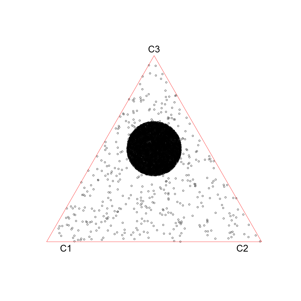
(a)

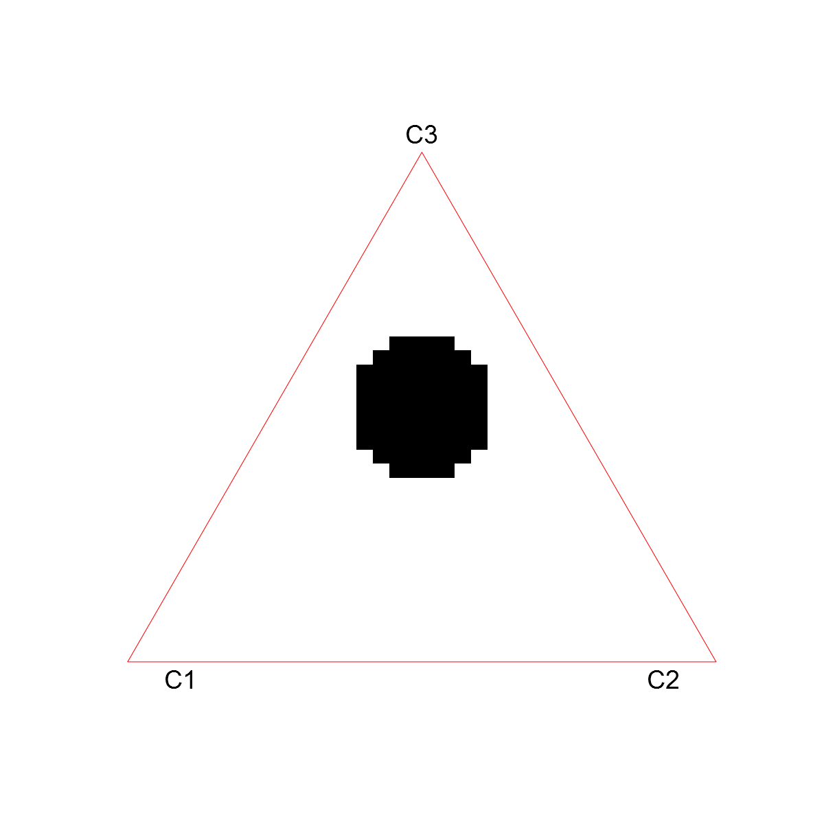
(b)

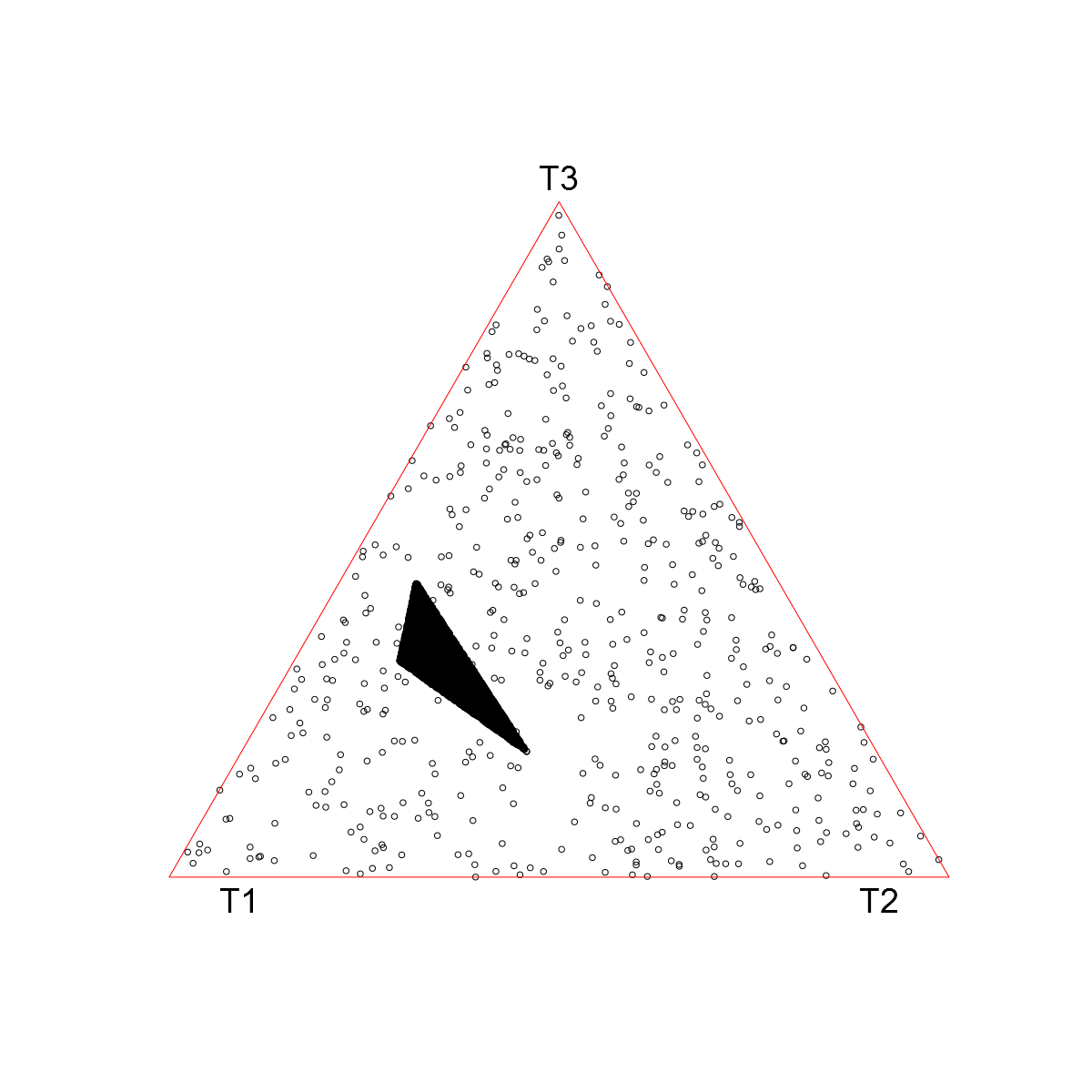
(c)

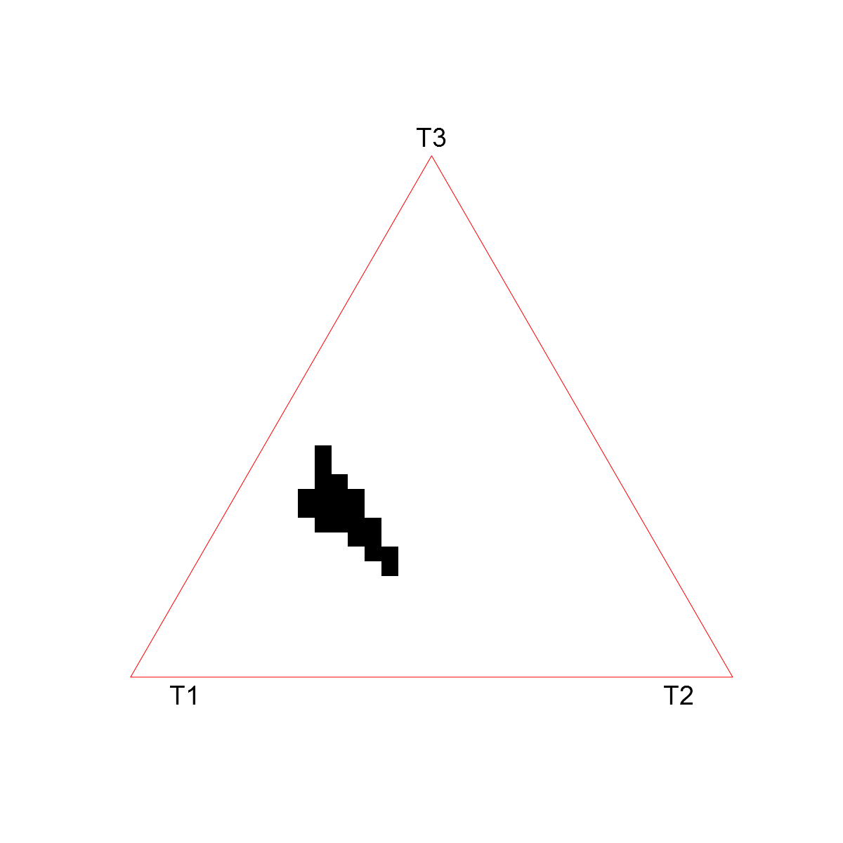
(d)

Figure 2: Figures present projected and estimated supports of simulated data. The large red triangles indicate the boundaries of the image of $C^{3}_{+}$ under a simplex mapping $T$ discussed in Section 1.6 and Example 1.2.

Figure 2 Illustrates how well the grid based support estimate is able to find the location of the set $B$. The dots in figures 2(a) and 2(c) are the projected $k=10000$ largest observations in $L_{1}$-norm. The dark dense region is the set $B$, which is a circle in 2(a) and a triangle in 2(c). In figures 2(b) and 2(d) the set $B$ is estimated by forming the support estimator ${\widehat{\textnormal{\bf{Tsupp}}}(k,m,q)}$ using parameter values $k=10000$, $m=36$ and $q=0.01$. Rejecting points with positive $q$ produces a clearly visible rasterized version of $B$ with no misidentified cells. This is due to the fact that our simulated data fits perfectly to the MRV framework.

The following examples show that real data produces less conclusive results.

4.2 Stock data vs. catastrophe fund

In this example, we study stock market dependencies using a data set consisting of daily prices of 6 stocks and a catastrophe fund. The studied securities and their ticker symbol abbreviations are: Google (GOOG), Microsoft (MSFT), Apple (AAPL), Chevron (CVX), Exxon (XOM), British Petrol (BP) and CATCo Reinsurance Opportunities Fund (CAT.L). Observations range from December 20, 2010 to 10 July, 2018. The data set was downloaded using the R-package Quantmod.

Observations were converted to log-returns by taking the logarithm of the price and calculating differences. Apart from CAT.L the resulting returns have similar tail indices for positive and negative tails. That is, the magnitudes of the estimated tail indices corresponding to the stock components are close to each other. However, the index of CAT.L was substantially smaller than the others, making it necessary to use the rank transform when comparing it against the other equities.

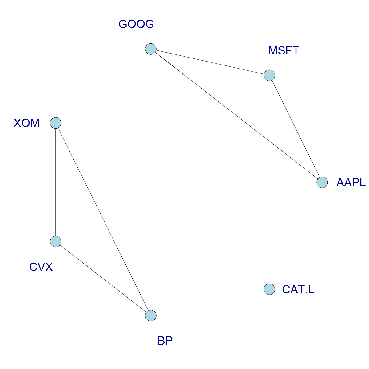
Figure 3: An exploratory graph illustrating the strongest preliminary pairwise asymptotic dependencies.

In Figure 3, the strength of pairwise dependence is calculated using the largest $k=200$ observations in $L_{1}$-norm projected to $C^{2}_{+}$, denoted $z_{1},z_{2},\ldots,z_{200}$, by

$$\left(\sum_{i=1}^{k}(1-d_{2}(1/2,z_{i}))\right)\Big{/}k.$$

That is, the dependence measure assigns pairs that have the largest distance to the midpoint $(1/2,1/2)$ of simplex $C^{2}_{+}$ small weights and pairs near the midpoint large weights. All pairwise dependencies that exceed the level $0.46$ are drawn as edges in Figure 3. The level was obtained empirically by gradually lowering the required level and observing which connections appeared on the graph first, that is, which dependencies were the strongest.

Figure 3 suggests that companies within the same financial sector, oil or technology, are probably not asymptotically independent but that the catastrophe fund might be asymptotically independent from stocks.

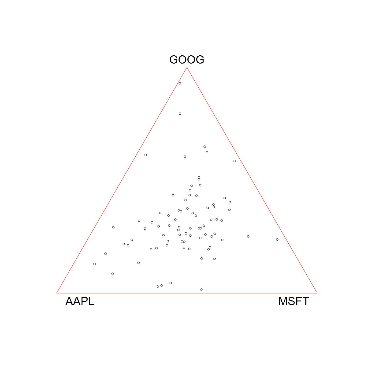
(a)

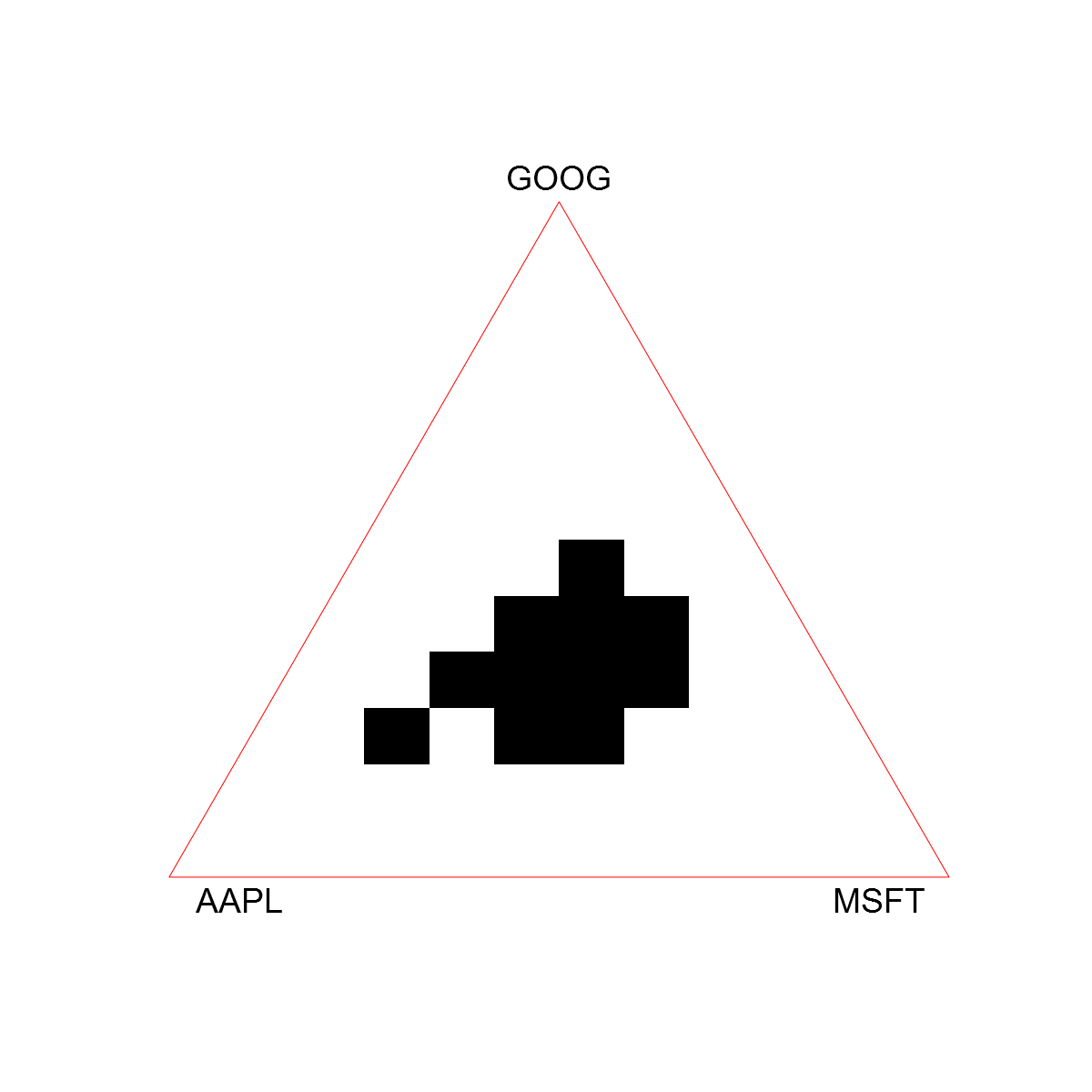
(b)

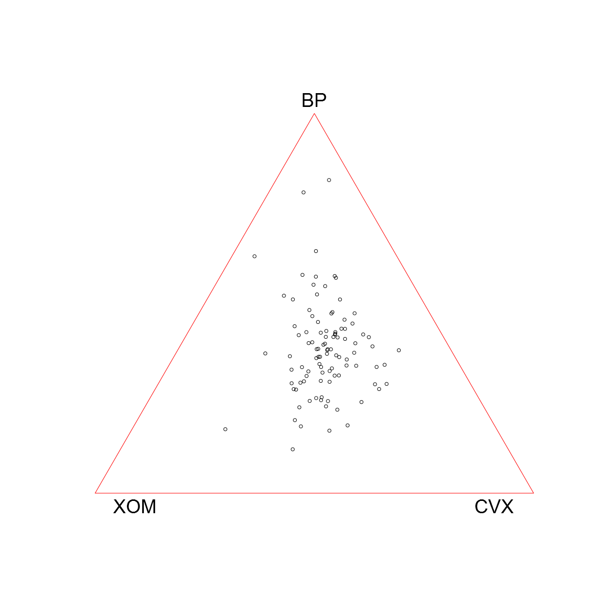
(c)

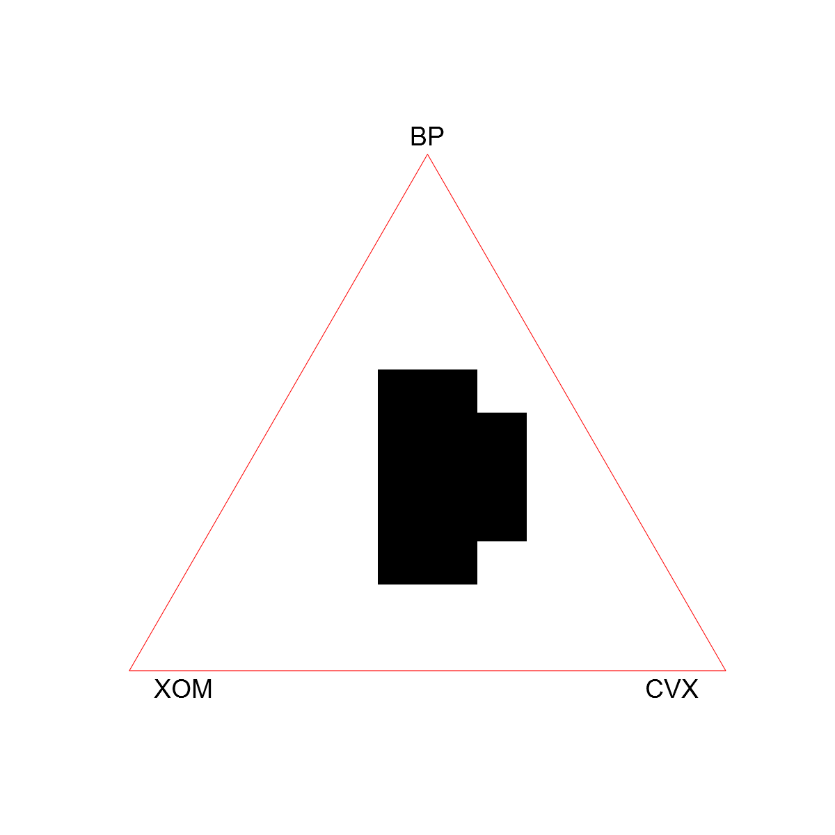
(d)

Figure 4: Projected largest $k=200$ observations and the estimated supports for tech stocks, in Figures 4(a)-4(b), and for oil stocks, in Figures 4(c)-4(d), respectively.

In Figure 4, projected and estimated supports of positive quadrants are depicted for oil and tech stocks. We used parameter values $k=200$, $m=12$ and $q=0.01$. Estimated grid based supports in subfigures 4(b) and 4(d) suggest that within a group, stock returns are not asymptotically independent and, in fact, exhibit fairly strong dependence. However, based on Figure 3 oil and tech sectors might be asymptotically independent and CAT.L could be asymptotically independent of all the studied stocks.

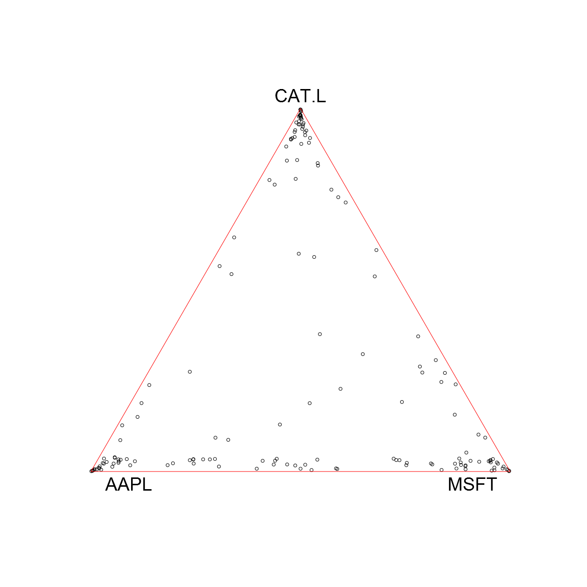
(a)

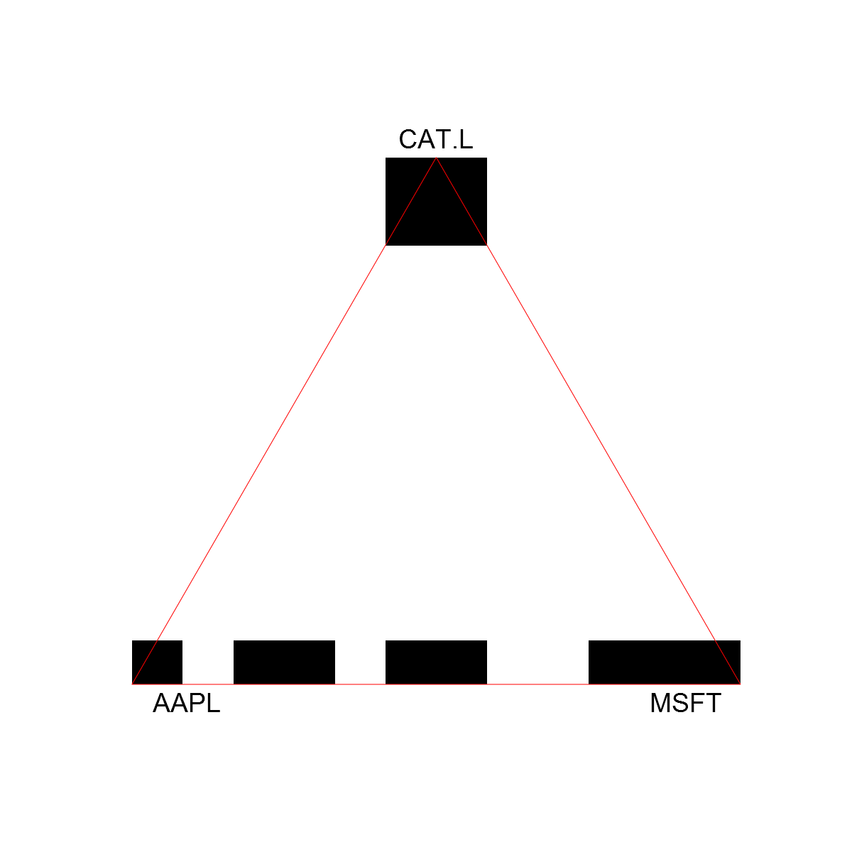
(b)

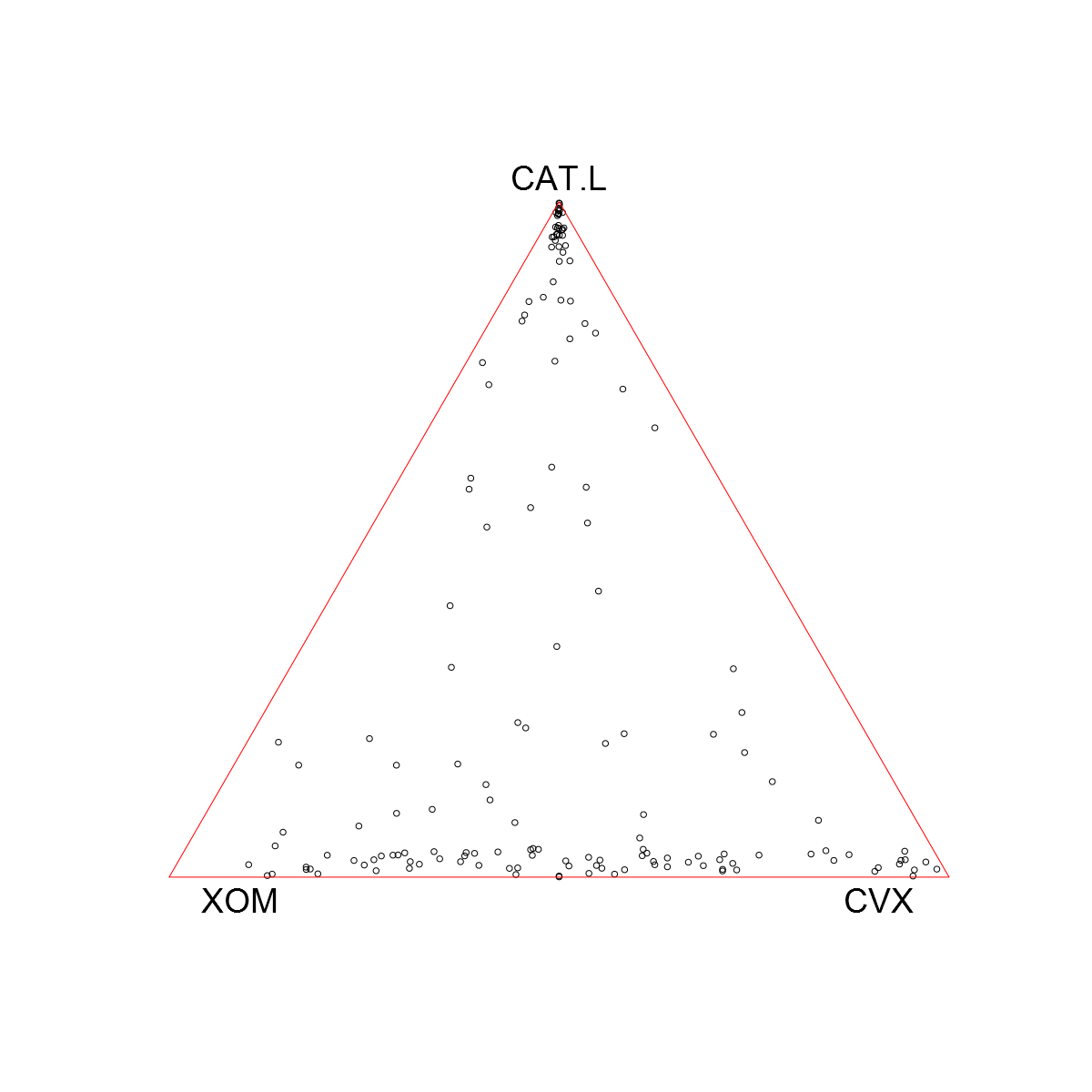
(c)

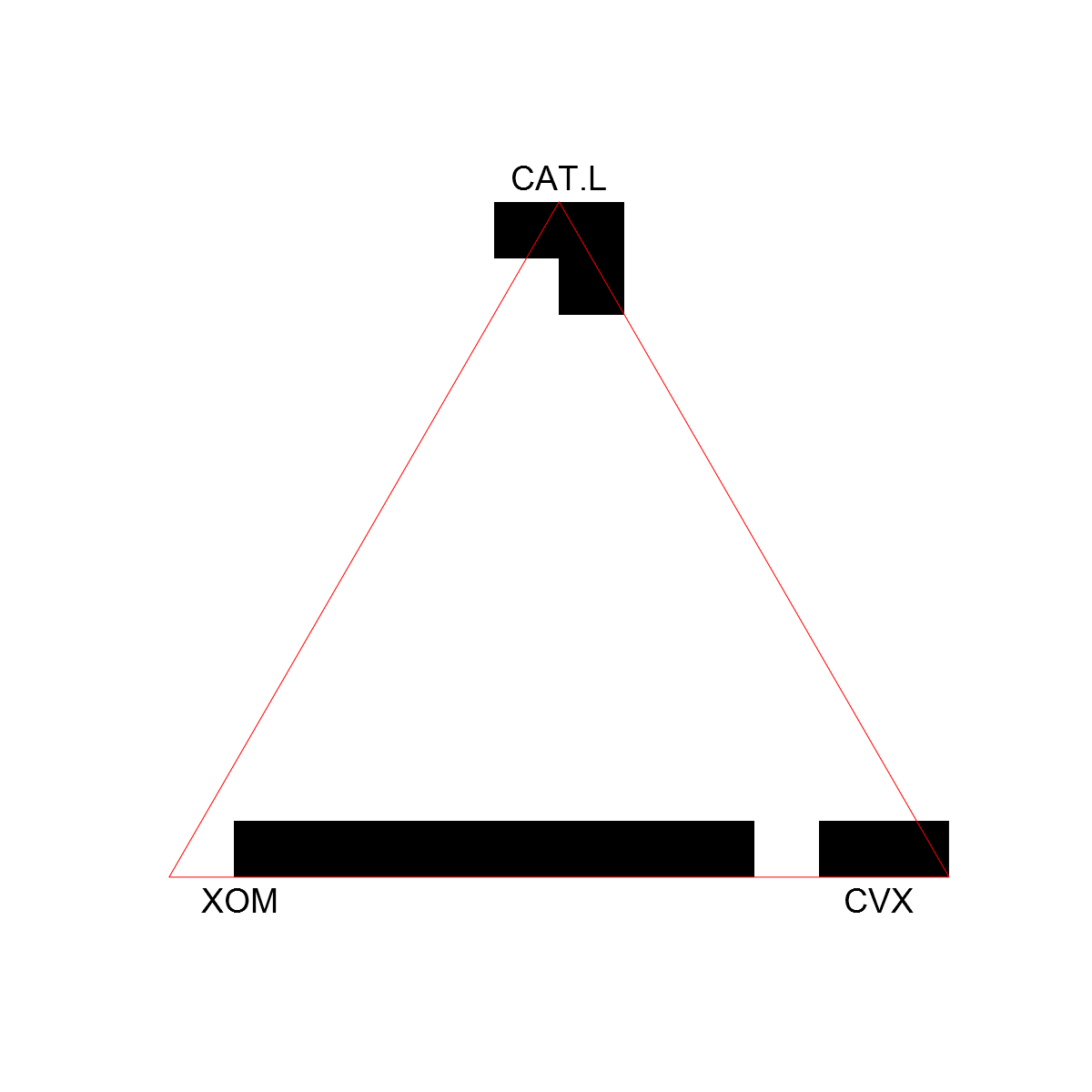
(d)

Figure 5: Projected and estimated supports of triples of stocks including CAT.L.

Asymptotic independence was tested using absolute values of observations. Test statistics were calculated based on the $k=50$ largest observations in $L_{1}$ norm. Function $g$ was defined for $m=2$. The intervals of Definition 3.4 were set to be of the form $a_{1}=0,b_{1}=c,a_{2}=1-c$ and $b_{2}=1$, where $c\in\{0,0.05,0.1\}$. That is, asymptotic independence was tested with and without buffers. In addition, it was assumed that $\mathbb{S}_{1}([0,c])=\mathbb{S}_{1}([1-c,1])=1/2$. Observations from first the oil and then the tech group were added together in order to form two dimensional vectors. The empirical test statistic $\hat{t}$ corresponding to $\hat{T}$ of (3.16) was formed in order to calculate the probability $\mathbb{P}(\hat{T}>|\hat{t}|)$ for different values of $c$. The approximate values of the probability were $2.58\cdot 10^{-5}$, $9.84\cdot 10^{-4}$ and $6.16\cdot 10^{-3}$ corresponding to $c=0$, $c=0.05$ and $c=0.1$, respectively. So, under the null hypothesis of asymptotic independence, there is significant evidence against asymptotic independence of the oil and tech sectors. This is a bit surprising given the preliminary observations of Figure 3.

Similar tests were performed pairwise with CAT.L against all $6$ stocks. There was insufficient evidence based on the test statistics corresponding to (3.16) to reject asymptotic independence. More precisely, Table 1 gives approximations for the probability $\mathbb{P}(\hat{T}>|\hat{t}|)$ for different values of $c$.

c	AAPL	MSFT	GOOG	XOM	CVX	BP
$0$	0.23	0.04	0.10	0.04	0.08	0.10
$0.05$	0.38	0.13	0.25	0.18	0.26	0.26
$0.1$	0.40	0.17	0.30	0.29	0.34	0.31

Table 1: Values of $\mathbb{P}(\hat{T}>|\hat{t}|)$ when the pairwise asymptotic independence of CAT.L and each of the $6$ stocks is studied. The column indicates which stock is tested against CAT.L. The row indicates which value of $c$ is used.

In conclusion, the test statistic developed in Section 3 supports the exploratory analysis of the preliminary dependence graph in Figure 3 in the sense that CAT.L seems to be asymptotically independent from the $6$ stocks. Asymptotic independence of the tech and oil sectors, however, was not strong enough to pass a more rigorous test.

4.3 FMI data

Daily rainfall data from three separate locations was downloaded from the Finnish Meteorological Institute. To reduce seasonal effects, we only used observations from summer months June, July and August and the total number of observations was $n=3864$. Two of the locations, Kouvola and Savonlinna are close to each other whereas the last one, Sodankylä, was further away. Rainfall in nearby locations showed high dependence. The rainfall at the further location, while not independent of the two others, exhibited extremal independence of the largest observations.

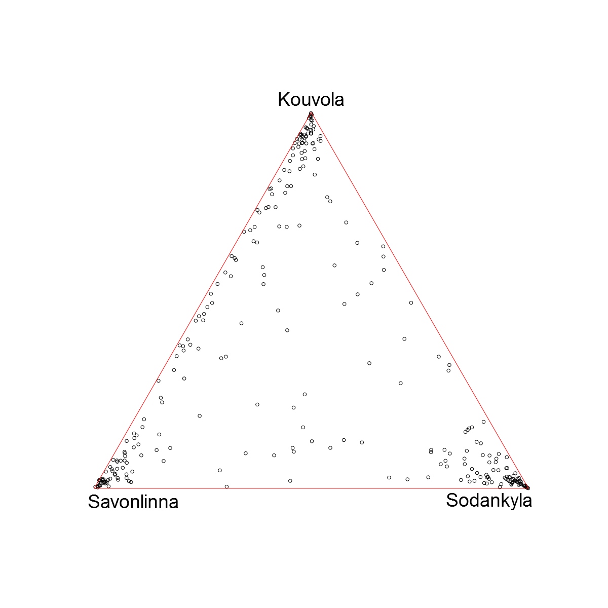
(a)

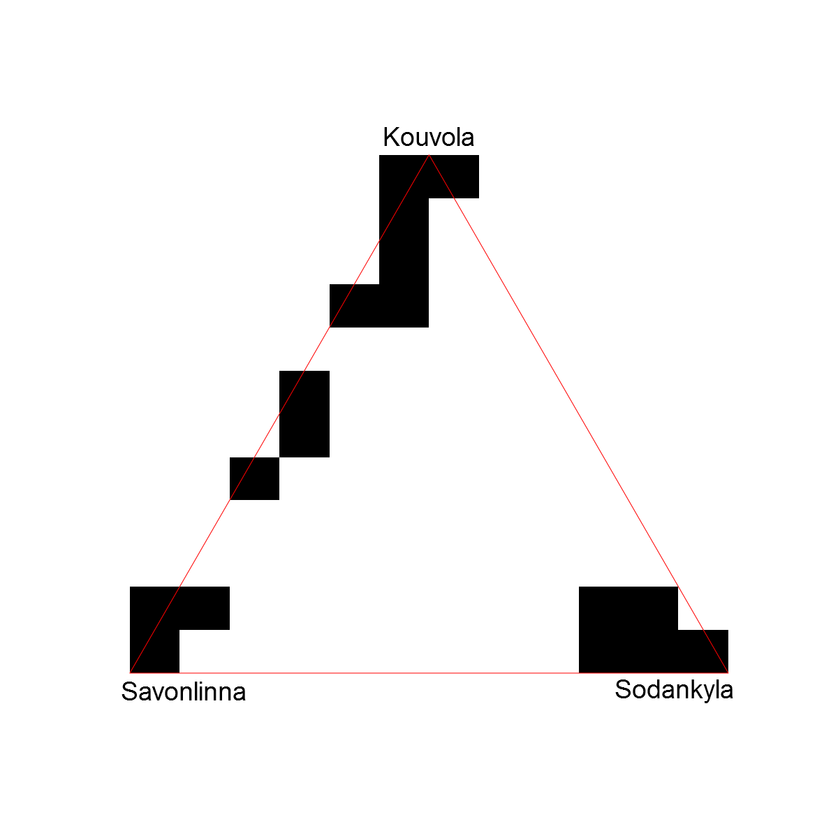
(b)

Figure 6: Projected and estimated supports of daily rainfall data recorded in 3 locations in Finland.

Figure 6 shows projected 3-dimensional points and estimated supports of the rank transformed rainfall vectors using $k=300$ largest observations. For the support estimate, we used parameter values $m=12$ and $q=0.01$. The rainfall data supports the idea that locations in close proximity (Savonlinna, Kouvola) are dependent and locations far away from each other are asymptotically independent.

4.4 Gold vs Silver price data

In this section, we study a data set consisting of daily gold and silver prices. The data is gathered from London Bullion Market Association. It is downloaded via the R-package Quandl. In the data, the price of one ounce of gold or silver is recorded each day during a time period ranging from December 3, 1973 to January 15, 2014. Only complete cases where the price information was available from both gold and silver were accepted as part of the data set. There were three days where price information was incomplete. Large price fluctuations did not occur during the omitted days and thus ignoring them has no effect to the resulting asymptotic analysis.

We transformed the daily price data to log-returns to obtain a sample which is better suited with the iid assumption of the model. The individual positive and negative marginals of gold and silver were reasonably heavy tailed. No power or rank transformations seemed necessary to standardize the data set. The resulting sample of $n=10323$ was thresholded by the $k=200$ largest observations in the $L_{1}$-norm and then projected onto $C^{2}$ to produce the diamond plot presented in Figure 7.

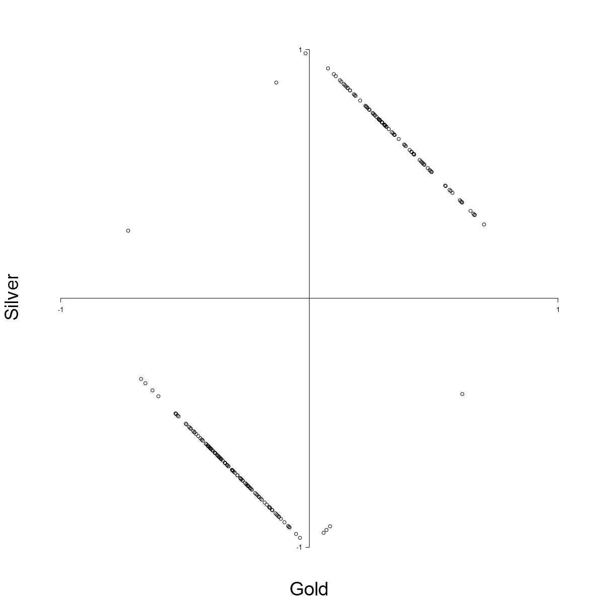
Figure 7: Diamond plot of daily price returns of gold and silver. The horizontal axis corresponds to gold and vertical axis to silver.

Figure 7 shows that the largest fluctuations in gold and silver prices tend to occur to the same direction. In addition, it seems that the points do not fill the positive or negative quadrant of the $C^{2}$ simplex evenly, but concentrate on intervals. The estimation of the asymptotic support in the negative quadrant was chosen as a suitable example, analysis of the other quadrants could be performed similarly. So, only the part of data where both components are negative was used. The $n=3951$ observations were multiplied by $-1$ to obtain a data set in the positive quadrant.

The one dimensional grid based estimator was obtained using the first $1975$ observations sampled uniformly without replacement from the data. The points were projected using a simplex mapping $T\colon C^{2}_{+}\to[0,1]$ defined by $T(x,y)=x$. Since gold is on the horizontal axis, the projected values on $[0,1]$ close to $0$ correspond to large losses in silver and values near $1$ correspond to large losses in gold prices.

The grid based support estimator with parameter values $n=1975$, $k=100$, $m=15$ and $q=0.02$ suggests that the asymptotic support should be covered by interval $[0,0.65]$.

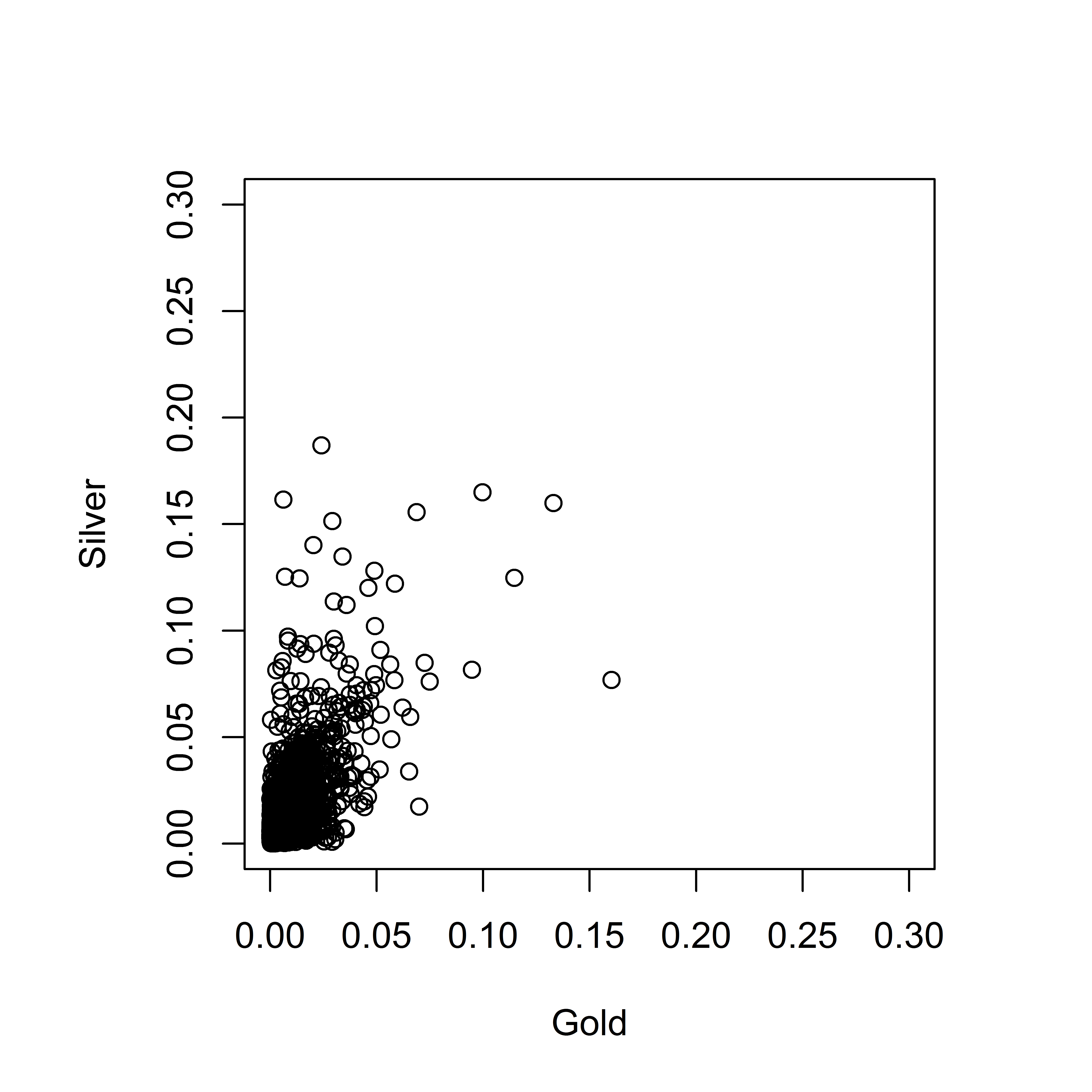
(a)

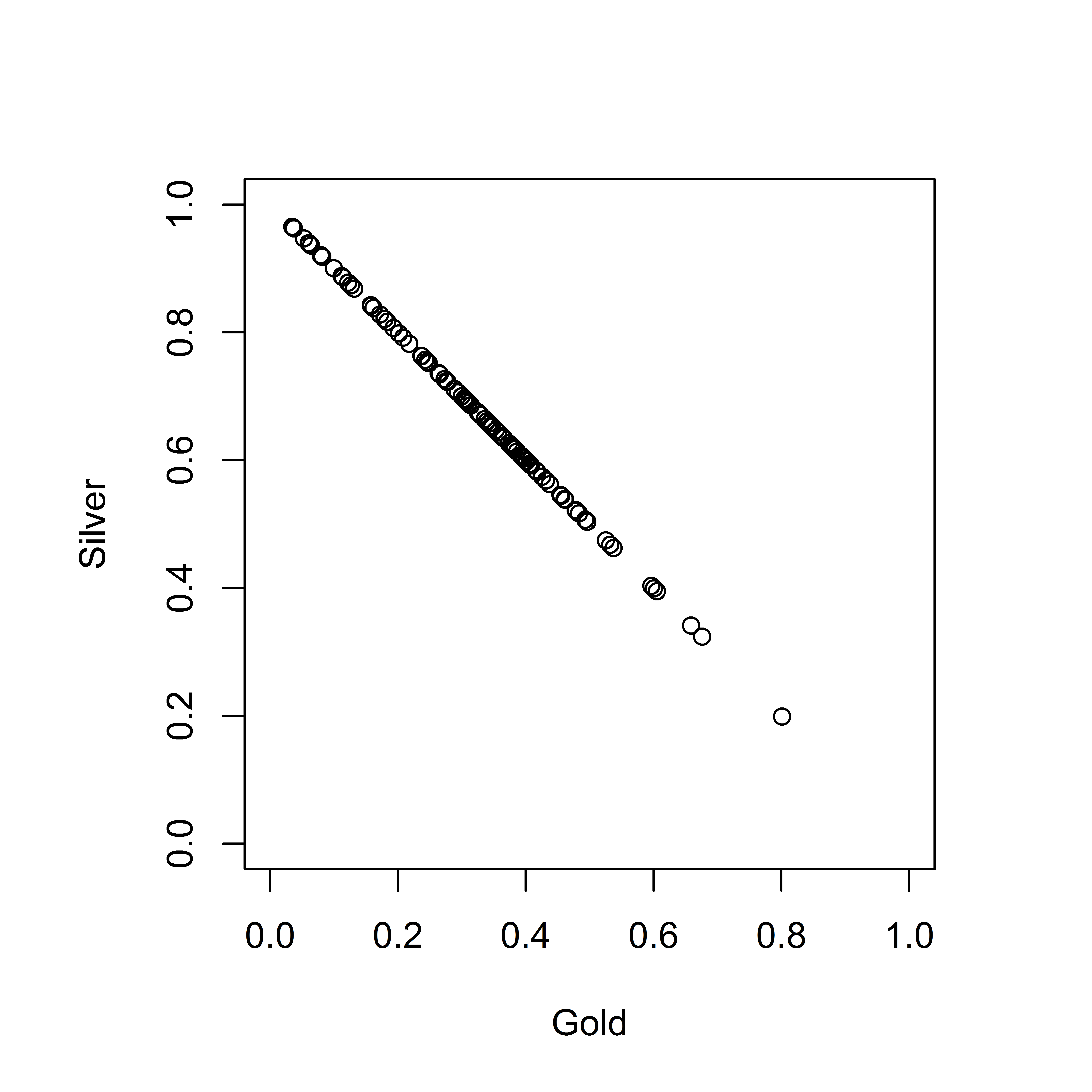
(b)

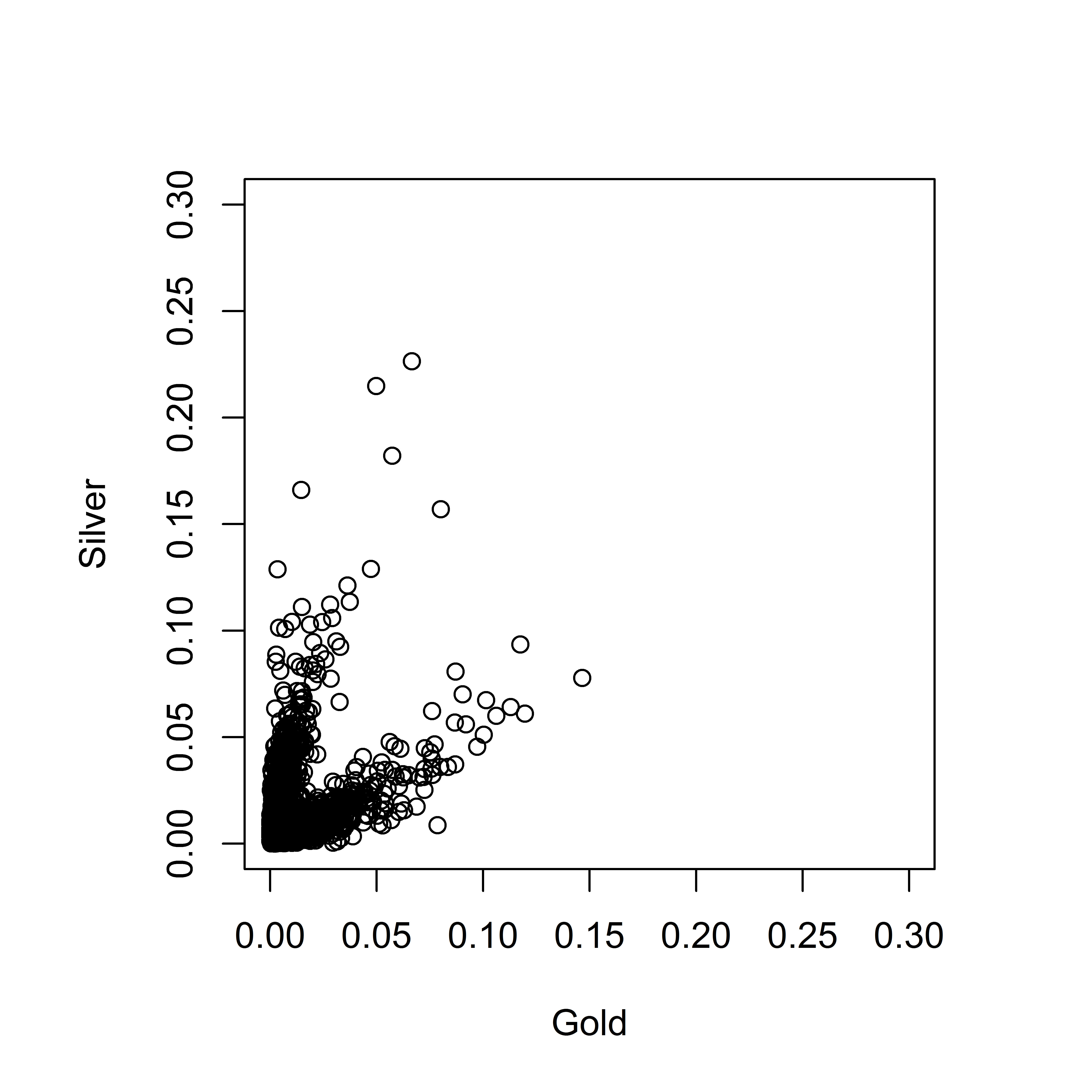
(c)

(d)

Figure 8: In Figure 8(a), the original data set is transformed using the method of Remark 3.5. The transformed observations are presented in Figure 8(c). Figures 8(b) and 8(d) show the diamond plot of the $k=100$ largest obervations in $L_{1}$ norm; Figure 8(b) corresponds to the data before application of the Remark 3.5 procedure and Figure 8(d) is after the procedure.

The validity of the support estimate was tested using the remaining $1976$ observations. Function $g$ was formed using the method of Remark 3.5. The process is illustrated in Figure 8. The aim is to test if the asymptotic support of the transformed data is covered by $[0,0.325]\cup[0.5,0.825]$. The null hypothesis is that in our sample $\hat{T}\sim N(0,1)$ where $\hat{T}$ is as in Equation (3.16). The empirical test statistic $\hat{t}$ corresponding to quantity $\hat{T}$ was calculated from the remaining observations with result $\hat{t}\approx 0.074$. Under the null hypothesis $\mathbb{P}(\hat{T}>|\hat{t}|)\approx 0.398$. So, the value of $\hat{t}$ gives no reason to reject the null hypothesis or the idea that the asymptotic support of the original sample is a subset of $[0,0.65]$.

As a practical application, we immediately obtain inequalities for large fluctuations in gold and silver prices. Denote the daily logarithmic decrease in prices with $x$ for gold and $y$ for silver. If a very large decrease is observed for gold, i.e. $x$ is large, then the support estimate implies $x/(x+y)\leq 0.65$ so that $y\geq 0.53x$. In other words, the support estimate says it is unlikely for the decrease in logarithmic silver price to be less than $0.53x$. So in the presence of extremal dependence, the method allows qualitative conclusions about otherwise unknown quantities.

4.5 Final thoughts

The examples show our methods are usable in some scenarios but asymptotic support estimation obviously has limitations. For one, it is challenging to find a large sample of vectors with tail equivalent marginals that satisfies the iid assumption. Thus, data pre-processing is required to get the data into usable form. With time series, larger number of observations may lead to poor results because of lack of stationarity. In financial contexts, a popular pre-processing method is de-GARCHing, see [29, Sec 2.1.]. The choice of pre-processing method adds a new source of uncertainty to the model.

Existence of an angular limit measure requires a standard MRV model in which marginal tails are tail equivalent. Theoretically, non-standard MRV models can be transformed to standard and the rank transform or power transform are the data analogues of the transform [49]. While rank transformed data can consistently estimate the limit measure [49, 28], it is not clear what effect such a transform applied to finite samples has on support estimation.

The proposed method in Sections 2 and 3 has an exploratory component since the support estimate requires choice of $k,m,q$. We are developing dedicated software that facilitates such choices and graphically shows effects of the choice on support identification and testing.

Acknowledgements

Jaakko Lehtomaa gratefully acknowledges hospitality and use of the services and facilities of Cornell University’s School of Operations Research and Information Engineering during his visit from Sep 2017 to Aug 2018, funded by the Finnish Cultural Foundation via the Foundations’ Post Doc Pool. Sidney Resnick was partially supported by US ARO MURI grant W911NF-12-1-0385 to Cornell University and final versions of this paper were written while visiting Australian National University’s College of Business and Economics and grateful acknowledgement is made for their hospitality and support.

References

- [1] Baillo, A., Cuevas, A., and Justel, A. Set estimation and nonparametric detection. Canadian Journal of Statistics 28, 4 (2000), 765–782.
- [2] Baíllo, A., and Cuevas, A. On the estimation of a star-shaped set. Advances in Applied Probability 33, 4 (2001), 717–726.
- [3] Biau, G., Cadre, B., Mason, D., and Pelletier, B. Asymptotic normality in density support estimation. Electron. J. Probab. 14 (2009), no. 91, 2617–2635.
- [4] Bräker, H., Hsing, T., and Bingham, N. H. On the Hausdorff distance between a convex set and an interior random convex hull. Adv. in Appl. Probab. 30, 2 (1998), 295–316.
- [5] Chevalier, J. Estimation du support et du contour du support d’une loi de probabilité. Ann. Inst. H. Poincaré Sect. B (NS) 12, 4 (1976), 339–364.
- [6] Clauset, A., Shalizi, C. R., and Newman, M. E. J. Power-law distributions in empirical data. SIAM Rev. 51, 4 (2009), 661–703.
- [7] Coles, S. An Introduction to Statistical Modeling of Extreme Values. Springer Series in Statistics. London: Springer. xiv, 210 p. , 2001.
- [8] Cooley, D., and Thibaud, E. Decompositions of Dependence for High-Dimensional Extremes. ArXiv e-prints (Dec. 2016).
- [9] Cuevas, A., Fraiman, R., et al. A plug-in approach to support estimation. The Annals of Statistics 25, 6 (1997), 2300–2312.
- [10] Das, B., Mitra, A., and Resnick, S. Living on the multidimensional edge: seeking hidden risks using regular variation. Adv. in Appl. Probab. 45, 1 (2013), 139–163.
- [11] Das, B., and Resnick, S. I. Models with hidden regular variation: generation and detection. Stoch. Syst. 5, 2 (2015), 195–238.
- [12] Das, B., and Resnick, S. I. Hidden regular variation under full and strong asymptotic dependence. Extremes 20, 4 (2017), 873–904.
- [13] Davis, R., and Mikosch, T. The extremogram: A correlogram for extreme events. Bernoulli 15, 4 (2009), 977–1009.
- [14] Davis, R., Mikosch, T., and Cribben, I. Towards estimating extremal serial dependence via the bootstrapped extremogram. Journal of Econometrics 170, 1 (2012), 142–152.
- [15] de Haan, L., and Ferreira, A. Extreme Value Theory: An Introduction. Springer-Verlag, New York, 2006.
- [16] de Haan, L., and Resnick, S. Estimating the limit distribution of multivariate extremes. Stochastic Models 9, 2 (1993), 275–309.
- [17] Devroye, L., and Wise, G. Detection of abnormal behavior via nonparametric estimation of the support. SIAM J. Appl. Math. 38, 3 (1980), 480–488.
- [18] Einmahl, J., de Haan, L., and Piterbarg, V. Nonparametric estimation of the spectral measure of an extreme value distribution. Ann. Statist. 29, 5 (2001), 1401–1423.
- [19] Einmahl, J. H. J., de Haan, L., and Sinha, A. K. Estimating the spectral measure of an extreme value distribution. Stochastic Process. Appl. 70, 2 (1997), 143–171.
- [20] Einmahl, J. H. J., and Segers, J. Maximum empirical likelihood estimation of the spectral measure of an extreme-value distribution. Ann. Statist. 37, 5B (2009), 2953–2989.
- [21] Embrechts, P., Hofert, M., and Wang, R. Bernoulli and tail-dependence compatibility. Ann. Appl. Probab. 26, 3 (2016), 1636–1658.
- [22] Embrechts, P., Klüppelberg, C., and Mikosch, T. Modelling extremal events, vol. 33 of Applications of Mathematics (New York). Springer-Verlag, Berlin, 1997. For insurance and finance.
- [23] Embrechts, P., Lindskog, F., and McNeil, A. Modelling dependence with copulas. Rapport technique, Département de mathématiques, Institut Fédéral de Technologie de Zurich, Zurich (2001).
- [24] Frahm, G., Junker, M., and Schmidt, R. Estimating the tail-dependence coefficient: properties and pitfalls. Insurance Math. Econom. 37, 1 (2005), 80–100.
- [25] Genest, C., Nešlehová, J. G., and Rivest, L.-P. The class of multivariate max-id copulas with -norm symmetric exponent measure. Bernoulli 24, 4B (2018), 3751–3790.
- [26] Gijbels, I., and Peng, L. Estimation of a support curve via order statistics. Extremes 3, 3 (2000), 251–277 (2001).
- [27] Goix, N., Sabourin, A., and Clémençon, S. Sparse representation of multivariate extremes with applications to anomaly detection. J. Multivariate Anal. 161 (2017), 12–31.
- [28] Heffernan, J., and Resnick, S. Hidden regular variation and the rank transform. Adv. Appl. Prob. 37, 2 (2005), 393–414.
- [29] Hofert, M., and Oldford, W. Visualizing dependence in high-dimensional data: An application to S&P 500 constituent data. Econometrics and Statistics (2017).
- [30] Joe, H. Multivariate models and dependence concepts, vol. 73 of Monographs on Statistics and Applied Probability. Chapman & Hall, London, 1997.
- [31] Joe, H. Dependence modeling with copulas, vol. 134 of Monographs on Statistics and Applied Probability. CRC Press, Boca Raton, FL, 2015.
- [32] Joe, H., and Li, H. Tail risk of multivariate regular variation. Methodology and Computing in Applied Probability (2010), 1–23. 10.1007/s11009-010-9183-x.
- [33] Kim, J. H., and Kim, J. A parametric alternative to the hill estimator for heavy-tailed distributions. Journal of Banking & Finance 54 (2015), 60 – 71.
- [34] Korostelev, A. P., Simar, L., and Tsybakov, A. B. Efficient estimation of monotone boundaries. The Annals of Statistics 23, 2 (1995), 476–489.
- [35] Larsson, M., and Resnick, S. I. Extremal dependence measure and extremogram: the regularly varying case. Extremes 15, 2 (2012), 231–256.
- [36] Lehtomaa, J. Limiting behaviour of constrained sums of two variables and the principle of a single big jump. Statist. Probab. Lett. 107 (2015), 157–163.
- [37] Lindskog, F., Resnick, S. I., and Roy, J. Regularly varying measures on metric spaces: hidden regular variation and hidden jumps. Probab. Surv. 11 (2014), 270–314.
- [38] Matheron, G. Random Sets and Integral Geometry. John Wiley & Sons, New York-London-Sydney, 1975. With a foreword by G.S. Watson, Wiley Series in Probability and Mathematical Statistics.
- [39] Matsui, M., and Mikosch, T. The extremogram and the cross-extremogram for a bivariate process. Adv. in Appl. Probab. 48, A (2016), 217–233.
- [40] McNeil, A. J., Frey, R., and Embrechts, P. Quantitative risk management, revised ed. Princeton Series in Finance. Princeton University Press, Princeton, NJ, 2015. Concepts, techniques and tools.
- [41] Meister, A. Support estimation via moment estimation in presence of noise. Statistics 40, 3 (2006), 259–275.
- [42] Mitra, A., and Resnick, S. Hidden regular variation and detection of hidden risks. Stochastic Models 27, 4 (2011), 591–614.
- [43] Mitra, A., and Resnick, S. Modeling multiple risks: hidden domain of attraction. Extremes 16, 4 (2013), 507–538.
- [44] Molchanov, I. Theory of Random Sets. Probability and its Applications (New York). Springer-Verlag London Ltd., London, 2005.
- [45] Nelsen, R. B. An introduction to copulas, second ed. Springer Series in Statistics. Springer, New York, 2006.
- [46] Peng, L. Estimation of the coefficient of tail dependence in bivariate extremes. Statist. Probab. Lett. 43, 4 (1999), 399–409.
- [47] Resnick, S. Hidden regular variation, second order regular variation and asymptotic independence. Extremes 5, 4 (2002), 303–336 (2003).
- [48] Resnick, S. The extremal dependence measure and asymptotic independence. Stoch. Models 20, 2 (2004), 205–227.
- [49] Resnick, S. I. Heavy-tail phenomena. Springer Series in Operations Research and Financial Engineering. Springer, New York, 2007. Probabilistic and statistical modeling.
- [50] Russell, B. T., Cooley, D. S., Porter, W. C., Reich, B. J., and Heald, C. L. Data mining to investigate the meteorological drivers for extreme ground level ozone events. Ann. Appl. Stat. 10, 3 (2016), 1673–1698.
- [51] Schölkopf, B., Platt, J. C., Shawe-Taylor, J. C., Smola, A. J., and Williamson, R. C. Estimating the support of a high-dimensional distribution. Neural Comput. 13, 7 (July 2001), 1443–1471.
- [52] Virkar, Y., and Clauset, A. Power-law distributions in binned empirical data. Ann. Appl. Stat. 8, 1 (2014), 89–119.