Contractions of the Maxwell algebra

Abstract

We construct all the possible non-relativistic, non-trivial, Galilei and Carroll k-contractions also known as k-1 p-brane contractions of the Maxwell algebra in $D+1$ space-time dimensions. $k$ has to do with the number of space-time dimensions one is contracting. For non-trivial solutions, we mean the ones with a non-abelian algebra of the momenta. We find in both cases, Galilei and Carroll, eight non trivial solutions. We also study the electromagnetic properties of the solutions, defined according to the scaling performed on the generators present in the Maxwell algebra. We find that besides the electric and magnetic contractions studied in the literature for $k=1$, that are related to the magnetic and electric limit of the free Maxwell equations, there also exist contractions where the two types of fields are scaled in the same way.

I Introduction

Relativistic particles coupled to a constant electro-magnetic (EM) field enjoy symmetries that extend the usual Poincaré algebra symmetries Bacry:1970ye , in this case the Lorentz generators $M_{\mu\nu}$ where $\mu,\nu=0,1\cdots D$, that preserve the given EM field span a two dimensional abelian group. Associating degrees of freedom to the constant EM field, one obtains a non-central extension of the Poincaré algebra generated by $M_{\mu\nu}$ and $P_{\mu}$, by an anti-symmetric tensor generator $Z_{\mu\nu}$. The resulting algebra has been called the Maxwell algebra in Schrader:1972zd . The generators of space-time translations become non-commuting, with commutators given by

$$[P_{\mu},P_{\nu}]=iZ_{\mu\nu},$$ (1)

with $Z_{\mu\nu}$ commuting with all $P_{\mu}$’s and among themselves. Of course, being a tensor the charges $Z_{\mu\nu}$ do not commute with the Lorentz generators: they transform covariantly under the Lorentz group. Therefore these charges are central for the translation group but not for the Poincaré group. Physically the Maxwell algebra was introduced as the symmetry of the covariant solutions of the Klein-Gordon field in a homogeneous classical electromagnetic field. The Maxwell group has been studied further, for example, in Beckers:1983gp ; negro1 ; Soroka:2004fj . The motion of a relativistic particle in a generic EM constant field, not fixed, was studied in Bonanos:2008ez assuming the Maxwell group as the symmetry of the model. It was also noticed that there are infinite extensions of the Maxwell algebra that are the symmetries of a particle in a generic EM field. The mathematical structure of these algebras has been elucidated in Gomis:2017cmt as a Free Lie algebra generated by the space-time translations generators $P_{\mu}$’s.

The motion of a non relativistic (NR) particle in a constant fixed EM field was considered in Bacry:1970du . The non-relativistic Maxwell algebras were studied in Beckers:1983gp ; negro2 ; Bonanos:2008kr . There are two types of NR Maxwell algebras that were obtained as magnetic and electric limit of the EM field. They are related to the two types of Galilean electromagnetism introduced in lebellac . In an algebraic way they correspond to two type of inequivalent contractions of the Maxwell algebra. Contractions of Lie groups and Lie algebras were introduced in Inonu:1953sp ; saletan .

Investigating the possible non-relativistic symmetry algebras is relevant for obtaining physical models with non-relativistic invariances. Beyond point particle dynamics, one can also consider realisations that lead to non-relativistic gravities Cartan1 ; Cartan2 ; Trautman63 ; Havas:1964zza ; DePietri:1994je ; Andringa:2010it ; Aviles:2018jzw ; Hansen:2018ofj ; Ozdemir:2019orp ; Hansen:2019vqf ; Bergshoeff:2019ctr ; Aviles:2019xed or even symmetries of extended objects such as strings and branes Gomis:2000bd ; Danielsson:2000gi ; Gomis:2005pg ; Brugues:2004an ; Brugues:2006yd ; Batlle:2016iel

In this paper we will study all the possible k-contractions also known as $k-1$-brane contractions of the Maxwell algebra. Here $k$ has to do with the number of space-time dimensions one is contracting, or scaling (see later for a more precise definition). We will be interested only in solutions leading to a non abelian algebra of the momenta. In fact, from a physical point of view, only in this case the charges $Z_{\mu\nu}$ lead to an interpretation in terms of an EM field Bonanos:2008ez . Therefore, we will define the case where the algebra of the momenta is abelian as a trivial one. In the trivial cases the algebraic structure is that of the contracted Poincaré algebra plus a set of charges with various behaviour with respect to the contracted boosts.

The magnetic and electric NR limits of the Maxwell equations studied in lebellac are related to to two particular cases of the $k=1$ contraction. These two different cases of non relativistic limit give rise to two different ways of performing the contraction, the magnetic and the electric contractions. When the magnetic field scales faster to infinity than the electric, we speak of a magnetic non-relativistic limit. In the opposite case, one speaks of electric non-relativistic limit. We will examine $k$ contractions of the Galilei and of the Carroll Levy-Leblond case. The two cases differ because in the Galilei case we scale k space variables, whereas for Carroll we scale the time variable plus k-1 space variables. For a generic $k$-contraction, in both cases we find 8 non trivial inequivalent contractions. With respect to the magnetic and electric cases we find 3 magnetic and 2 electric solutions, whereas in the remaining 3, the electric and the magnetic fields are scaled in the same way. In the particular case of $k=1$ for the Galilei case there are only 3 non trivial solutions. These 3 cases are one electric, one magnetic and one with equal scaling.

The contracted Maxwell algebras we found can have interesting extensions. If we would like to obtain these algebras by contraction we will need to enlarge the Maxwell algebra. In the case of three dimensions for k=1 these were studied in Aviles:2018jzw by introducing U(1) factors. In this paper we will not consider the general situation.

In the Carroll case all the 8 solutions are present for $k=1$. However, for $k=D$, the situation is similar to Galilei for $k=1$, that is, only 3 solutions lead to a non-abelian algebra of the momenta. On the other hand, all these solutions are now of an electric type.

This paper is organised as follows: in Section II we resume our method to obtain the contractions of the Poincaré group (see Barducci:2018wuj ). Furthermore we introduce the most general contractions (or scaling) of the charges $Z_{\mu\nu}$ compatible with the rotational invariance. The contractions of the charges depend on three exponents. The determination of these three parameters is going to fix the non trivial inequivalent solutions for the contractions of the Maxwell algebra with no central charges, both in the Galilei and in the Carroll cases. In Section III we study the $k$-contractions of the Galilei type leading to non trivial contractions. In Section IIIA we study these contracted algebras in coordinate space giving the explicit expressions for the generators of the contracted generators. An analogous study is done in Sections IV and IVA for the Carroll case. Conclusions are in Section V. In the Appendix A we discuss the equivalence of two possible contractions for the Galilei case, but the same argument can be applied to Carroll. In Appendix B we prove that the definitions used for the contracted charges are the most general compatible with the rotational invariance.

II Description of the $k$-contractions

In this Section we will study the $k$-contractions of Galilei and Carroll type of the Maxwell algebra. In the case of the Poincaré algebra this was done in Barducci:2018wuj . The Maxwell algebra in $D+1$ space-time dimensions has $(D+1)^{2}$ generators: $M_{\mu\nu},P_{\mu},Z_{\mu\nu}$, with commutation relations Schrader:1972zd

$$\left[M_{\mu\nu},M_{\rho\sigma}\right] = i(\eta_{\mu\rho}M_{\nu\sigma}+\eta_{\nu\sigma}M_{\mu\rho}-\eta_{\mu\sigma}M_{\nu\rho}-\eta_{\nu\rho}M_{\mu\sigma}),$$

$$\left[M_{\mu\nu},P_{\rho}\right] = i(\eta_{\mu\rho}P_{\nu}-\eta_{\nu\rho}P_{\mu}),$$

$$\left[P_{\mu},P_{\nu}\right] = iZ_{\mu\nu},$$

$$\left[M_{\mu\nu},Z_{\rho\sigma}\right] = i(\eta_{\mu\rho}Z_{\nu\sigma}+\eta_{\nu\sigma}Z_{\mu\rho}-\eta_{\nu\rho}Z_{\mu\sigma}-\eta_{\mu\sigma}Z_{\nu\rho}),$$

$$\left[Z_{\mu\nu},Z_{\rho\sigma}\right] = \left[Z_{\mu\nu},P_{\rho}\right]=0,$$ (2)

with $\eta_{\mu\nu}=(-;+,\cdots,+)$ and $\mu,\nu=0,1,...,D$.

A property that will be useful in the following is that the Maxwell algebra is invariant under the following rescaling

$$M_{\mu\nu}\to\alpha^{0}M_{\mu\nu},~{}~{}~{}P_{\mu}\to\alpha^{1}P^{\mu}.~{}~{}~{}Z_{\mu\nu}\to\alpha^{2}Z_{\mu\nu},$$ (3)

the exponents of the scaling of the generators correspond to the level of the generators in the Free Lie algebra description of Maxwell algebras Gomis:2017cmt . The generator of this scaling is the generator $D$ of the dilatations.

Since the momenta are not commuting, the quadratic Casimir $P^{2}$ is modified Schrader:1972zd , see also Soroka:2004fj Gomis:2009dm . Its expression is:

$$C_{2}=P^{2}+M_{\mu\nu}Z^{\mu\nu}.$$ (4)

In order to define the $k$ contractions of the Maxwell algebra we proceed as in Barducci:2018wuj by partitioning the $D+1$ dimensional space-time in a $k$ dimensional Minkowskian part and in a $D+1-k$ dimensional Euclidean one (for the case $k=1$ see also Beckers:1983gp ; Aviles:2018jzw ) by introducing the following set of labels for the space-time coordinates

$$\alpha,\beta=0,1,\cdots,k-1,~{}~{}~{}\eta_{\alpha\beta}=(-;+,\cdots,+),$$

$$a,b=k,\cdots,D,~{}~{}~{}\eta_{ab}=(+,+,\cdots,+).$$ (5)

Let us recall how the $k$-contractions have been defined in Barducci:2018wuj ; Barducci:2018thr for the Poincaré case, (see also Brugues:2004an ; Gomis:2005pg ; Brugues:2006yd ). We have to consider the following two subgroups of $ISO(1,D)$: the Poincaré subgroup in $k$ dimensions, $ISO(1,k-1)$ and the euclidean group of roto-translations in $D+1-k$ dimensions, generated respectively by

$$ISO(1,k-1):~{}~{}~{}M_{\alpha\beta},~{}~{}P_{\alpha},~{}~{}~{}\alpha,\beta=0,1,\cdots,k-1,$$ (6)

$$ISO(D+1-k):~{}~{}~{}M_{ab},~{}~{}P_{a},~{}~{}~{}a,b=k,\cdots,D.$$ (7)

In these notations the generators of $ISO(1,D)$ are

$$ISO(1,D):~{}~{}~{}M_{\alpha\beta},~{}~{}~{}M_{ab},~{}~{}P_{\alpha},~{}~{}~{}P_{a},~{}~{}~{}M_{\alpha b}\equiv B_{\alpha b}.$$ (8)

Note that the boosts $B_{\alpha b}$ connect the two subalgebras.

In Barducci:2018wuj we have considered two types of contractions, both at the level of the Poincaré algebra and at the level of the invariant vector fields . These contractions generalise the Carroll Levy-Leblond ; Bergshoeff:2014jla ; Duval:2014uoa ; Cardona:2016ytk and the Galilei algebras LL Gomis:2000bd ; Danielsson:2000gi ; Brugues:2004an ; Gomis:2005pg ; Brugues:2006yd Batlle:2016iel ; Gomis:2016zur ; Batlle:2017cfa . We note that we will be interested in the cases of Galilei and Carroll symmetries with no central charges.

At the Lie algebra level the contractions are made on the momenta and on the boosts as follows

$${\rm Galilei}:\tilde{P}_{a}={\displaystyle\frac{1}{\omega}}P_{a},~{}~{}~{}\tilde{B}_{\alpha a}={\displaystyle\frac{1}{\omega}}B_{\alpha a},$$ (9)

$${\rm Carroll}:\tilde{P}_{\alpha}={\displaystyle\frac{1}{\omega}}P_{\alpha},~{}~{}~{}\tilde{B}_{\alpha a}={\displaystyle\frac{1}{\omega}}B_{\alpha a}.$$ (10)

and taking the limit $\omega\to\infty$. The tilde generators will be the ones associated to the ”non-relativistic” algebras. The resulting algebra is

$${\rm Galilei}:[\tilde{B}_{\alpha a},\tilde{B}_{\beta c}]=0,~{}~{}~{}[\tilde{B}_{\alpha a},\tilde{P}_{\beta}]=i\eta_{\alpha\beta}\tilde{P}_{a},~{}~{}~{}[\tilde{B}_{\alpha a},\tilde{P}_{b}]=0,$$ (11)

$${\rm Carroll}:[\tilde{B}_{\alpha a},\tilde{B}_{\beta b}]=0,~{}~{}~{}[\tilde{B}_{\alpha a},\tilde{P}_{\beta}]=0,~{}~{}~{}[\tilde{B}_{\alpha a},\tilde{P}_{b}]=-i\eta_{ab}\tilde{P}_{\alpha}.$$ (12)

Since the Poincaré algebra is invariant under a global rescaling of the momenta, the previous definition of the contractions is equivalent to:

$${\rm Galilei}:\tilde{P}_{\alpha}=\omega P_{\alpha},~{}~{}~{}\tilde{B}_{\alpha a}={\displaystyle\frac{1}{\omega}}B_{\alpha a},$$ (13)

$${\rm Carroll}:\tilde{P}_{a}=\omega P_{a},~{}~{}~{}\tilde{B}_{\alpha a}={\displaystyle\frac{1}{\omega}}B_{\alpha a}.$$ (14)

In the Maxwell case we have seen that the algebra is invariant under the rescaling given in eq. (3). It follows that also in this case the contractions defined in eqs. (13) and (14) are equivalent to the ones in eqs. (9) and (10). An explicit proof for the Galilei case is given in Appendix A. This proof can be simply extended to the Carroll case

We will complete the $k$-contraction of the Maxwell algebra through the following definition of the contracted charges $Z_{\mu\nu}$ that will be used both in the Galilei and the Carroll case:

$$\tilde{Z}_{ab}=\omega^{t}Z_{ab},~{}~{}~{}\tilde{Z}_{a\alpha}=\omega^{r}Z_{a\alpha},~{}~{}~{}\tilde{Z}_{\alpha\beta}=\omega^{s}Z_{\alpha\beta}.$$ (15)

This definition of the contracted charges is unique if we want to preserve the covariance in the Minkowski and in the Euclidean sectors of the space-time.

Let us note that the possible values of the three exponents $t,r,s$ will fix the possible contractions for the Maxwell algebra.

In the following two Sections we will consider the Galilei and the Carroll cases separately.

III Classification of the $k$-contractions for the Galilei case

In this Section we will determine the values of the exponents $t,r,s$ of eq. (15) leading to a finite contracted algebra in the limit $\omega\to\infty$. The relevant commutators to be considered to this end are the following:

$$[\tilde{P}_{a},\tilde{P}_{b}]=\frac{i}{\omega^{2}}Z_{ab}=\frac{i}{\omega^{t+2}}\tilde{Z}_{ab}\to t+2\geq 0,$$ (16)

$$[\tilde{P}_{a},\tilde{P}_{\alpha}]=\frac{i}{\omega}Z_{a\alpha}=\frac{i}{\omega^{r+1}}\tilde{Z}_{a\alpha}\to r+1\geq 0,$$ (17)

$$[\tilde{P}_{\alpha},\tilde{P}_{\beta}]=iZ_{\alpha\beta}=\frac{i}{\omega^{s}}\tilde{Z}_{\alpha\beta},\to s\geq 0,$$ (18)

where we have used (13) and (15). Let us note that whenever one of the exponents$,t,r,s$ is strictly greater than the values obtained in the previous equations, the commutators of the corresponding momenta vanish in the limit $\omega\to\infty$, that is

$$t>-2\to[\tilde{P}_{a}.\tilde{P}_{b}]=0,$$

$$r>-1\to[\tilde{P}_{a}.\tilde{P}_{\alpha}]=0.$$

$$s>0\to[\tilde{P}_{\alpha}.\tilde{P}_{\beta}]=0.$$ (19)

Therefore, the contractions corresponding to all the values of the exponents $t,r,s$ greater than the previous values are trivial, in the sense specified in the Introduction.

Let us now consider the commutators of the boosts with the tensor charges. We have:

$$[\tilde{B}_{\alpha a},\tilde{Z}_{bc}]=\frac{1}{\omega^{1-t}}[B_{\alpha a},Z_{bc}]=\frac{i}{\omega^{1-t+r}}\left(\eta_{ac}\tilde{Z}_{\alpha b}-\eta_{ab}\tilde{Z}_{\alpha c}\right)\to 1-t+r\geq 0,$$ (20)

$$[\tilde{B}_{\alpha a},\tilde{Z}_{b\beta}]=\frac{1}{\omega^{1-r}}[B_{\alpha a},Z_{b\beta}]=-\frac{i}{\omega^{1-r}}\left(\eta_{\alpha\beta}\omega^{-t}\tilde{Z}_{ab}+\eta_{ab}\omega^{-s}\tilde{Z}_{\alpha\beta}\right)\to 1-r+t\geq 0,1-r+s\geq 0,$$ (21)

$$[\tilde{B}_{\alpha a},\tilde{Z}_{\beta\gamma}]=\frac{1}{\omega^{1-s}}[B_{\alpha a},Z_{\beta\gamma}]=\frac{i}{\omega^{1-s}}\left(\eta_{\alpha\beta}\omega^{-r}\tilde{Z}_{a\gamma}-\eta_{\alpha\gamma}\omega^{-r}\tilde{Z}_{a\beta}\right)\to 1+r-s\geq 0,$$ (22)

It follows:

$$-1\leq r-t\leq+1,~{}~{}~{}-1\leq r-s\leq+1.$$ (23)

The allowed regions for the parameters are shown in Fig. 1, and are the ones to the right of the vertical lines, $t=-2$ and $s=0$, in the upper part of the horizontal line $r=-1$ and in between the two diagonal lines:

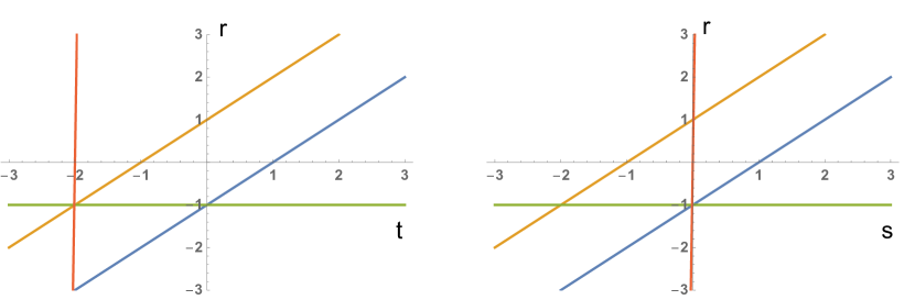
Figure 1: The lines delimiting regions allowed for the contractions in the Galilei case. In the left-panel, $r$ vs. $t$. In the right one, $r$ vs. $s$.

By inspection it is easy to find all the solutions leading to non vanishing commutators among all the momenta. We find 8 solutions that are listed in Table 1. Note that these 8 solutions reduce to 3 non-trivial ones, in the case $k=1$, due to the vanishing of the tensor $\tilde{Z}_{\alpha\beta}$. For all the other values of the triple $t,r,s$ the algebra of the momenta becomes abelian.

Of course, there are infinite trivial solutions with the tensor charges having different commutation relations with the boosts $\tilde{B}_{\alpha a}$ and with $\tilde{M}_{ab}$ and $\tilde{M}_{\alpha\beta}$.

Notice that it is possible to obtain non-vanishing commutators of the tensor charges with the boosts, whenever the parameters $t,r,s$ are at the borders of the regions inside the diagonal lines in Fig. 1. Without entering into a very detailed discussion, we list the four possibilities of having at least one commutator of the boosts with the charges different from zero:
$r-t=-1$

$$[\tilde{B}_{\alpha a},\tilde{Z}_{bc}]=i\left(\eta_{ac}\tilde{Z}_{\alpha b}-\eta_{ab}\tilde{Z}_{\alpha c}\right)\equiv C^{1}_{\alpha a;bc},$$ (24)

$r-t=+1,~{}r-s\not=1$

$$[\tilde{B}_{\alpha a},\tilde{Z}_{b\beta}]=-i\eta_{\alpha\beta}\tilde{Z}_{ab}\equiv C^{2}_{\alpha a;b\beta},$$ (25)

$r-s=+1,~{}r-t\not=1$

$$[\tilde{B}_{\alpha a},\tilde{Z}_{b\beta}]=-i\eta_{ab}\tilde{Z}_{\alpha\beta}\equiv C^{3}_{\alpha a;b\beta},$$ (26)

$r-s=-1$

$$[\tilde{B}_{\alpha a},\tilde{Z}_{\beta\gamma}]=i\left(\eta_{\alpha\beta}\tilde{Z}_{a\gamma}-\eta_{\alpha\gamma}\tilde{Z}_{a\beta}\right)\equiv C^{4}_{\alpha a;\beta\gamma}.$$ (27)

In Table 1 we also list the relevant commutators for the 8 solutions of the exponents $t,r,s$.

Table 1: The commutators for the inequivalent $k$ contractions of Galilei type of the Maxwell algebra

$~{}n^{0}~{}$	$t$	$r$	s	$r-t$	$r-s$	$[\tilde{P}_{a},\tilde{P}_{b}]$	$[\tilde{P}_{\alpha},\tilde{P}_{a}]$	$[\tilde{P}_{\alpha},\tilde{P}_{\beta}]$	$[\tilde{B}_{\alpha a},\tilde{Z}_{bc}]$	$[\tilde{B}_{\alpha a},\tilde{Z}_{b\beta}]$	$[\tilde{B}_{\alpha a},\tilde{Z}_{\beta\gamma}]$
1	-2	-1	0	+1	-1	$i\tilde{Z}_{ab}$	$i\tilde{Z}_{\alpha a}$	$i\tilde{Z}_{\alpha\beta}$	0	$C^{2}_{\alpha a;b\beta}$	$C^{4}_{\alpha a;\beta\gamma}$
2	-1	-1	0	0	-1	$0$	$i\tilde{Z}_{\alpha a}$	$i\tilde{Z}_{\alpha\beta}$	0	0	$C^{4}_{\alpha a;\beta\gamma}$
3	-1	0	0	+1	0	$0$	$0$	$i\tilde{Z}_{\alpha\beta}$	0	$C^{2}_{\alpha a;b\beta}$	0
4	0	-1	0	-1	-1	$0$	$i\tilde{Z}_{\alpha a}$	$i\tilde{Z}_{\alpha\beta}$	$C^{1}_{\alpha a;bc}$	0	$C^{4}_{\alpha a;\beta\gamma}$
5	0	0	0	0	0	$0$	$0$	$i\tilde{Z}_{\alpha\beta}$	0	0	0
6	0	1	0	+1	+1	$0$	$0$	$i\tilde{Z}_{\alpha\beta}$	0	$C^{2}_{\alpha a;b\beta}+C^{3}_{\alpha a;b\beta}$	0
7	1	0	0	-1	0	$0$	$0$	$i\tilde{Z}_{\alpha\beta}$	$C^{1}_{\alpha a;bc}$	0	0
8	1	1	0	0	+1	$0$	$0$	$i\tilde{Z}_{\alpha\beta}$	0	$C^{3}_{\alpha a;b\beta}$	0

where the coefficients $C^{i}$ are given in eqs. (24)$-$(27).

In the case $k=1$ the only non trivial inequivalent contractions, in the sense that they lead to a non abelian algebra of the momenta, are those corresponding to the solutions 1), 2) and 4).

We are now in the position to analyse in a more detailed way the so called magnetic and electric contractions that we discussed in the Introduction. In the case $k=1$, we have the following charges: $Z_{ab}$ and $Z_{a0}$ corresponding respectively to magnetic and electric fields. In the usual way of discussing the non relativistic limit, one scales the finite charges. In our case the finite charges are the tilde ones. Therefore we need to consider the limit $\omega\to\infty$ of the expressions

$$Z_{ab}=\omega^{-t}\tilde{Z}_{ab},~{}~{}~{}~{}Z_{a0}=\omega^{-s}\tilde{Z}_{a0}.$$ (28)

We obtain the magnetic case when $-t>-r$ and the electric case in the opposite case. In other words, the magnetic and the electric case are discriminated by the values of $r-t$. By looking at Table 1 we see that this quantity may assume three values, $\pm 1$ and $0$, magnetic case corresponding to $r-t=+1$ and the electric case to $r-t=-1$. However we see that another case is possible, namely the case where electric and magnetic field scale in the same way. This will be called the EM case.

By extension, also for $k\not=1$ we will define magnetic, electric and EM the cases corresponding to the three possible values of $r-t$. In the case $k=1$ we have only three non trivial contractions of all the three types. For a generic $k$, there are three magnetic solutions, two electric and three EM.

III.1 $k$-contractions in configuration space

We will now consider the $k$-contractions in the configuration space spanned by the coordinates of the coset space Maxwell/Lorentz,. The generic element of the coset space will be written as (see ref. Bonanos:2008ez )

$$g=e^{iP_{\mu}x^{\mu}}e^{\frac{i}{2}Z_{\mu\nu}\theta^{\mu\nu}},$$ (29)

with $\theta^{\mu\nu}=-\theta^{\nu\mu}$. Therefore, our configuration space will be parameterised by $x^{\mu}$ and $\theta^{\mu\nu}$. The vector fields generating the Lorentz group transformations are given by:

$$M_{\mu\nu}=i~{}(x_{\mu}\frac{\partial}{\partial x^{\nu}}-x_{\nu}\frac{\partial}{\partial x^{\mu}}+{\theta_{\mu}}^{\lambda}\frac{\partial}{\partial\theta^{\nu\lambda}}-{\theta_{\nu}}^{\lambda}\frac{\partial}{\partial\theta^{\mu\lambda}}),$$ (30)

whereas the vector fields corresponding to $Z_{\mu\nu}$ and $P_{\mu}$ are (see ref. Bonanos:2008ez )

$$Z_{\mu\nu} = -i~{}\frac{\partial}{\partial\theta^{\mu\nu}},$$

$$P_{\mu} = -i~{}(\frac{\partial}{\partial x^{\mu}}-\frac{1}{2}x^{\nu}\frac{\partial}{\partial\theta^{\mu\nu}})..$$ (31)

We note that the vector fields of eqs. (30) and (31) are the so-called right-invariant vector fields generating the opposite Maxwell algebra, implying that the right hand side of the commutation relations has the opposite sign.

The contractions on the coordinates are obtained by the inverse scaling with respect to the corresponding generators, that is, in the Galilei case:

$$\tilde{x}^{a}=\omega x^{a},~{}~{}~{}\tilde{\theta}^{ab}=\omega^{-t}\theta^{ab},~{}~{}~{}\tilde{\theta}^{\alpha a}=\omega^{-r}\theta^{\alpha a},~{}~{}~{}\tilde{\theta}^{\alpha\beta}=\omega^{-s}\theta^{\alpha\beta},$$ (32)

Using eqs. (30), (31) and (32) we find

$$\tilde{Z}_{\mu\nu} = -i~{}\frac{\partial}{\partial\tilde{\theta}^{\mu\nu}},$$ (33)

$$\tilde{P}_{a} = -i~{}(\frac{\partial}{\partial\tilde{x}^{a}}-\frac{1}{2(\omega^{2+t})}\tilde{x}^{b}\frac{\partial}{\partial\tilde{\theta}^{ab}}-\frac{1}{2(\omega^{1+r})}\tilde{x}^{\beta}\frac{\partial}{\partial\tilde{\theta}^{a\beta}}),$$ (34)

$$\tilde{P}_{\alpha} = -i~{}(\frac{\partial}{\partial\tilde{x}^{\alpha}}-\frac{1}{2(\omega^{1+r})}\tilde{x}^{b}\frac{\partial}{\partial\tilde{\theta}^{\alpha b}}-\frac{1}{2(\omega^{s})}\tilde{x}^{\beta}\frac{\partial}{\partial\tilde{\theta}^{\alpha\beta}}),$$ (35)

$$\tilde{B}_{\alpha a} = i\left(\tilde{x}_{\alpha}\frac{\partial}{\partial\tilde{x}^{a}}-\frac{\tilde{\theta}_{a}^{.\,b}}{\omega^{1+r-t}}\frac{\partial}{\partial\tilde{\theta}^{\alpha b}}-\frac{\tilde{\theta}_{a}^{.\,\beta}}{\omega^{1-r+s}}\frac{\partial}{\partial\tilde{\theta}^{\alpha\beta}}+\frac{\tilde{\theta}_{\alpha}^{.\,b}}{\omega^{1-r+t}}\frac{\partial}{\partial\tilde{\theta}^{ab}}+\frac{\tilde{\theta}_{\alpha}^{.\,\beta}}{\omega^{1-s+r}}\frac{\partial}{\partial\tilde{\theta}^{a\beta}}\right),$$ (36)

$$\tilde{M}_{\alpha\beta} = M_{\alpha\beta}(x\to\tilde{x},\theta\to\tilde{\theta}),$$ (37)

$$\tilde{M}_{ab} = M_{ab}(x\to\tilde{x},\theta\to\tilde{\theta}),$$ (38)

In the following Table 2 we give the expressions of the generators of the contracted algebra for the 8 solutions we previously found.

Table 2: The generators of the contracted Maxwell algebras in configuration space

$~{}n^{0}~{}$	$t$	$r$	s	$r-t$	$r-s$	$\tilde{P}_{a}$	$\tilde{P}_{\alpha}$	$\tilde{B}_{a\alpha}$
1	-2	-1	0	+1	-1	$-i~{}(\frac{\partial}{\partial\tilde{x}^{a}}-\frac{1}{2}\tilde{x}^{\mu}\frac{\partial}{\partial\tilde{\theta}^{a\mu}})$	$-i~{}(\frac{\partial}{\partial\tilde{x}^{\alpha}}-\frac{1}{2}\tilde{x}^{\mu}\frac{\partial}{\partial\tilde{\theta}^{\alpha\mu}})$	$i\left(\tilde{x}_{\alpha}\frac{\partial}{\partial\tilde{x}^{a}}+\tilde{\theta}_{\alpha}^{.\,b}\frac{\partial}{\partial\tilde{\theta}^{ab}}+\tilde{\theta}_{\alpha}^{.\,\beta}\frac{\partial}{\partial\tilde{\theta}^{a\beta}}\right)$
2	-1	-1	0	0	-1	$-i~{}(\frac{\partial}{\partial\tilde{x}^{a}}-\frac{1}{2}\tilde{x}^{\beta}\frac{\partial}{\partial\tilde{\theta}^{a\beta}})$	$-i~{}(\frac{\partial}{\partial\tilde{x}^{\alpha}}-\frac{1}{2}\tilde{x}^{\mu}\frac{\partial}{\partial\tilde{\theta}^{\alpha\mu}})$	$i\left(\tilde{x}_{\alpha}\frac{\partial}{\partial\tilde{x}^{a}}+\tilde{\theta}_{\alpha}^{.\,\beta}\frac{\partial}{\partial\tilde{\theta}^{a\beta}}\right)$
3	-1	0	0	+1	0	$-i\frac{\partial}{\partial\tilde{x}^{a}}$	$-i(\frac{\partial}{\partial\tilde{x}^{\alpha}}-\frac{1}{2}\tilde{x}^{\beta}\frac{\partial}{\partial\tilde{\theta}^{\alpha\beta}})$	$i\left(\tilde{x}_{\alpha}\frac{\partial}{\partial\tilde{x}^{a}}+\tilde{\theta}_{\alpha}^{.\,b}\frac{\partial}{\partial\tilde{\theta}^{ab}}\right)$
4	0	-1	0	-1	-1	$-i(\frac{\partial}{\partial\tilde{x}^{a}}-\frac{1}{2}\tilde{x}^{\beta}\frac{\partial}{\partial\tilde{\theta}^{a\beta}})$	$-i~{}(\frac{\partial}{\partial\tilde{x}^{\alpha}}-\frac{1}{2}\tilde{x}^{\mu}\frac{\partial}{\partial\tilde{\theta}^{\alpha\mu}})$	$i\left(\tilde{x}_{\alpha}\frac{\partial}{\partial\tilde{x}^{a}}-\tilde{\theta}_{a}^{.\,b}\frac{\partial}{\partial\tilde{\theta}^{\alpha b}}+\tilde{\theta}_{\alpha}^{.\,\beta}\frac{\partial}{\partial\tilde{\theta}^{a\beta}}\right)$
5	0	0	0	0	0	$-i\frac{\partial}{\partial\tilde{x}^{a}}$	$-i(\frac{\partial}{\partial\tilde{x}^{\alpha}}-\frac{1}{2}\tilde{x}^{\beta}\frac{\partial}{\partial\tilde{\theta}^{\alpha\beta}})$	$i\tilde{x}_{\alpha}\frac{\partial}{\partial\tilde{x}^{a}}$
6	0	1	0	+1	+1	$-i\frac{\partial}{\partial\tilde{x}^{a}}$	$-i(\frac{\partial}{\partial\tilde{x}^{\alpha}}-\frac{1}{2}\tilde{x}^{\beta}\frac{\partial}{\partial\tilde{\theta}^{\alpha\beta}})$	$i\left(\tilde{x}_{\alpha}\frac{\partial}{\partial\tilde{x}^{a}}-\tilde{\theta}_{a}^{.\,\beta}\frac{\partial}{\partial\tilde{\theta}^{\alpha\beta}}+\tilde{\theta}_{\alpha}^{.\,b}\frac{\partial}{\partial\tilde{\theta}^{ab}}\right)$
7	1	0	0	-1	0	$-i\frac{\partial}{\partial\tilde{x}^{a}}$	$-i(\frac{\partial}{\partial\tilde{x}^{\alpha}}-\frac{1}{2}\tilde{x}^{\beta}\frac{\partial}{\partial\tilde{\theta}^{\alpha\beta}})$	$-i\left(-\tilde{x}_{\alpha}\frac{\partial}{\partial\tilde{x}^{a}}+\tilde{\theta}_{a}^{.\,b}\frac{\partial}{\partial\tilde{\theta}^{\alpha b}}\right)$
8	1	1	0	0	+1	$-i\frac{\partial}{\partial\tilde{x}^{a}}$	$-i(\frac{\partial}{\partial\tilde{x}^{\alpha}}-\frac{1}{2}\tilde{x}^{\beta}\frac{\partial}{\partial\tilde{\theta}^{\alpha\beta}})$	$i\left(\tilde{x}_{\alpha}\frac{\partial}{\partial\tilde{x}^{a}}-\tilde{\theta}_{a}^{.\,\beta}\frac{\partial}{\partial\tilde{\theta}^{\alpha\beta}}\right)$

With this Table we conclude the classification of the $k$-contractions of the Maxwell algebra with no central charges for the Galilei case.

IV Classification of the $k$-contractions for the Carroll case

We will now examine the Carroll case. The $k$-contraction is defined by eq. (10)

$$\tilde{P}_{\alpha}={\displaystyle\frac{1}{\omega}}P_{\alpha},~{}~{}~{}\tilde{B}_{\alpha a}={\displaystyle\frac{1}{\omega}}B_{\alpha a}.$$ (40)

The other possibility of contractions as in eq. (14) can be shown to give the same results, following the same lines discussed in Appendix A for the Galilei case.

The relevant commutation relations for the Carroll generators are

$$[\tilde{B}_{\alpha a},\tilde{B}_{\beta b}]=0,~{}~{}~{}[\tilde{B}_{\alpha a},\tilde{P}_{\beta}]=0,~{}~{}~{}[\tilde{B}_{\alpha a},\tilde{P}_{b}]=-i\eta_{ab}\tilde{P}_{\alpha}.$$ (41)

We define the contracted tensor charges as in the Galilei case:

$$\tilde{Z}_{ab}=\omega^{t}Z_{ab},~{}~{}~{}\tilde{Z}_{a\alpha}=\omega^{r}Z_{a\alpha},~{}~{}~{}\tilde{Z}_{\alpha\beta}=\omega^{s}Z_{\alpha\beta}.$$ (42)

Again, in order to get a well defined contracted algebra we impose the following requirements:

$$[\tilde{P}_{a},\tilde{P}_{b}]=iZ_{ab}=\frac{i}{\omega^{t}}\tilde{Z}_{ab}\to t\geq 0,$$ (43)

$$[\tilde{P}_{a},\tilde{P}_{\alpha}]=\frac{i}{\omega}Z_{a\alpha}=\frac{i}{\omega^{r+1}}\tilde{Z}_{a\alpha}\to r+1\geq 0,$$ (44)

$$[\tilde{P}_{\alpha},\tilde{P}_{\beta}]=\frac{i}{\omega^{2}}Z_{\alpha\beta}=\frac{i}{\omega^{s+2}}\tilde{Z}_{\alpha\beta},\to s+2\geq 0.$$ (45)

As for the commutators of the Carroll boosts with the tensor charges we get the same results as in eqs. (20), (21) and (22):

$$[\tilde{B}_{\alpha a},\tilde{Z}_{bc}]=\frac{1}{\omega^{1-t}}[B_{\alpha a},Z_{bc}]=\frac{i}{\omega^{1-t+r}}\left(\eta_{ac}\tilde{Z}_{\alpha b}-\eta_{ab}\tilde{Z}_{\alpha c}\right)\to 1-t+r\geq 0,$$ (46)

$$[\tilde{B}_{\alpha a},\tilde{Z}_{b\beta}]=\frac{1}{\omega^{1-r}}[B_{\alpha a},Z_{b\beta}]=-\frac{i}{\omega^{1-r}}\left(\eta_{\alpha\beta}\omega^{-t}\tilde{Z}_{ab}+\eta_{ab}\omega^{-s}\tilde{Z}_{\alpha\beta}\right)\to 1-r+t\geq 0,1-r+s\geq 0,$$ (47)

$$[\tilde{B}_{\alpha a},\tilde{Z}_{\beta\gamma}]=\frac{1}{\omega^{1-s}}[B_{\alpha a},Z_{\beta\gamma}]=\frac{i}{\omega^{1-s}}\left(\eta_{\alpha\beta}\omega^{-r}\tilde{Z}_{a\gamma}-\eta_{\alpha\gamma}\omega^{-r}\tilde{Z}_{a\beta}\right)\to 1+r-s\geq 0,$$ (48)

from which

$$-1\leq r-t\leq+1,~{}~{}~{}-1\leq r-s\leq+1.$$ (49)

The allowed regions are shown in Fig. 2, and are the ones to the right of the vertical lines, $t=0$ and $s=-2$, the one in the upper part of the horizontal line $r=-1$ and in between the two diagonal lines.

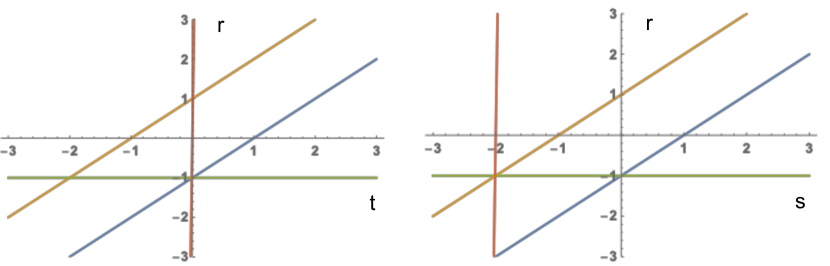
Figure 2: The lines delimiting regions allowed for the contractions in the Carroll case. In the left-panel, $r$ vs. $t$. In the right one, $r$ vs. $s$.

From this we conclude that the non trivial solutions of the previous inequalities for the exponents $t,r,s$ of this case, can be obtained by looking at the solutions for the Galilei case with the exchange $s\leftrightarrow t$. Therefore we can use the Table 1 of the Galilei case, by performing the substitution $s$ with $t$. At the same time, it is clear from eqs. (43) and (45) that we need to perform the exchange $\tilde{Z}_{ab}\leftrightarrow\tilde{Z}_{\alpha\beta}$, and of the corresponding commutators among the momenta, in Table 1. Also, exchanging $s$ with $t$ the differences $r-t$ and $r-s$ are exchanged, implying a corresponding change in the commutators with the boosts, according to the eqs. (24)$-$(27). Taking everything into account, we obtain the Table 3.

We note that contrarily to the Galilei case, where for $k=1$ only 3 non trivial solutions were surviving, in the Carroll case, for $k=1$ all the 8 solutions are non trivial. However. in the present case the non trivial solutions reduce to 3 for $k=D$, since then $Z_{ab}=0$.

As for the electric and magnetic behaviour, in the Carroll case there are 3 electric solutions, 2 magnetic and 3 EM. Therefore the number of the electric and magnetic solutions are exchanged with respect to the Galilei case. In ref. Duval:2014uoa only the electric and magnetic case were considered for $k=1$

Table 3: The commutators for the inequivalent $k$ contractions of Carroll type of the Maxwell algebra

$~{}n^{0}~{}$	$s$	$r$	t	$r-s$	$r-t$	$[\tilde{P}_{a},\tilde{P}_{b}]$	$[\tilde{P}_{\alpha},\tilde{P}_{a}]$	$[\tilde{P}_{\alpha},\tilde{P}_{\beta}]$	$[\tilde{B}_{\alpha a},\tilde{Z}_{bc}]$	$[\tilde{B}_{\alpha a},\tilde{Z}_{b\beta}]$	$[\tilde{B}_{\alpha a},\tilde{Z}_{\beta\gamma}]$
1	-2	-1	0	+1	-1	$i\tilde{Z}_{ab}$	$i\tilde{Z}_{\alpha a}$	$i\tilde{Z}_{\alpha\beta}$	$C^{1}_{\alpha a;bc}$	$C^{3}_{\alpha a;b\beta}$	$0$
2	-1	-1	0	0	-1	$i\tilde{Z}_{ab}$	$i\tilde{Z}_{\alpha a}$	$0$	$C^{1}_{\alpha a;bc}$	0	$0$
3	-1	0	0	+1	0	$i\tilde{Z}_{ab}$	$0$	$0$	0	$C^{3}_{\alpha a;b\beta}$	0
4	0	-1	0	-1	-1	$i\tilde{Z}_{ab}$	$i\tilde{Z}_{\alpha a}$	$0$	$C^{1}_{\alpha a;bc}$	0	$C^{4}_{\alpha a;\beta\gamma}$
5	0	0	0	0	0	$i\tilde{Z}_{ab}$	$0$	$0$	0	0	0
6	0	1	0	+1	+1	$i\tilde{Z}_{ab}$	$0$	$0$	0	$C^{2}_{\alpha a;b\beta}+C^{3}_{\alpha a;b\beta}$	0
7	1	0	0	-1	0	$i\tilde{Z}_{ab}$	$0$	$0$	$0$	0	$C^{4}_{\alpha a;\beta\gamma}$
8	1	1	0	0	+1	$i\tilde{Z}_{ab}$	$0$	$0$	0	$C^{2}_{\alpha a;b\beta}$	0

IV.1 Configuration space

The contracted variables in configuration space are:

$$\tilde{x}^{\alpha}=\omega x^{\alpha},~{}~{}~{}\tilde{\theta}^{ab}=\omega^{-t}\theta^{ab},~{}~{}~{}\tilde{\theta}^{\alpha a}=\omega^{-r}\theta^{\alpha a},~{}~{}~{}\tilde{\theta}^{\alpha\beta}=\omega^{-s}\theta^{\alpha\beta},$$ (50)

and the expressions for the generators are:

$$\tilde{Z}_{\mu\nu} = -i~{}\frac{\partial}{\partial\tilde{\theta}^{\mu\nu}},$$ (51)

$$\tilde{P}_{a} = -i~{}(\frac{\partial}{\partial\tilde{x}^{a}}-\frac{1}{2(\omega^{t})}\tilde{x}^{b}\frac{\partial}{\partial\tilde{\theta}^{ab}}-\frac{1}{2(\omega^{1+r})}\tilde{x}^{\beta}\frac{\partial}{\partial\tilde{\theta}^{a\beta}}),$$ (52)

$$\tilde{P}_{\alpha} = -i~{}(\frac{\partial}{\partial\tilde{x}^{\alpha}}-\frac{1}{2(\omega^{1+r})}\tilde{x}^{b}\frac{\partial}{\partial\tilde{\theta}^{\alpha b}}-\frac{1}{2(\omega^{2+s})}\tilde{x}^{\beta}\frac{\partial}{\partial\tilde{\theta}^{\alpha\beta}}),$$ (53)

$$\tilde{B}_{\alpha a} = i\left(-\tilde{x}_{a}\frac{\partial}{\partial\tilde{x}^{\alpha}}-\frac{\tilde{\theta}_{a}^{.\,b}}{\omega^{1+r-t}}\frac{\partial}{\partial\tilde{\theta}^{\alpha b}}-\frac{\tilde{\theta}_{a}^{.\,\beta}}{\omega^{1-r+s}}\frac{\partial}{\partial\tilde{\theta}^{\alpha\beta}}+\frac{\tilde{\theta}_{\alpha}^{.\,b}}{\omega^{1-r+t}}\frac{\partial}{\partial\tilde{\theta}^{ab}}+\frac{\tilde{\theta}_{\alpha}^{.\,\beta}}{\omega^{1-s+r}}\frac{\partial}{\partial\tilde{\theta}^{a\beta}}\right),$$ (54)

$$\tilde{M}_{\alpha\beta} = M_{\alpha\beta}(x\to\tilde{x},\theta\to\tilde{\theta}),$$ (55)

$$\tilde{M}_{ab} = M_{ab}(x\to\tilde{x},\theta\to\tilde{\theta}),$$ (56)

In Table 4 we give the expressions for the generators in configuration space for the various solutions. This concludes the classification of the $k$-contractions of the Maxwell algebra with no central charges in the Carroll case

Table 4: The generators of the contracted Maxwell algebras in configuration space for the Carroll case

$~{}n^{0}~{}$	$s$	$r$	t	$r-s$	$r-t$	$\tilde{P}_{a}$	$\tilde{P}_{\alpha}$	$\tilde{B}_{a\alpha}$
1	-2	-1	0	+1	-1	$-i~{}(\frac{\partial}{\partial\tilde{x}^{a}}-\frac{1}{2}\tilde{x}^{\mu}\frac{\partial}{\partial\tilde{\theta}^{a\mu}})$	$-i~{}(\frac{\partial}{\partial\tilde{x}^{\alpha}}-\frac{1}{2}\tilde{x}^{\mu}\frac{\partial}{\partial\tilde{\theta}^{\alpha\mu}})$	$-i(\tilde{x}_{a}\frac{\partial}{\partial\tilde{x}^{\alpha}}+{\tilde{\theta}_{a}^{.\,b}}\frac{\partial}{\partial\tilde{\theta}^{\alpha b}}+{\tilde{\theta}_{a}^{.\,\beta}}\frac{\partial}{\partial\tilde{\theta}^{\alpha\beta}})$
2	-1	-1	0	0	-1	$-i~{}(\frac{\partial}{\partial\tilde{x}^{a}}-\frac{1}{2}\tilde{x}^{\mu}\frac{\partial}{\partial\tilde{\theta}^{a\mu}})$	$-i(\frac{\partial}{\partial\tilde{x}^{\alpha}}-\frac{1}{2}\tilde{x}^{b}\frac{\partial}{\partial\tilde{\theta}^{\alpha b}})$	$-i\left(\tilde{x}_{a}\frac{\partial}{\partial\tilde{x}^{\alpha}}+{\tilde{\theta}_{a}^{.\,b}}\frac{\partial}{\partial\tilde{\theta}^{\alpha b}}\right)$
3	-1	0	0	+1	0	$-i~{}\left(\frac{\partial}{\partial\tilde{x}^{a}}-\frac{1}{2}\tilde{x}^{b}\frac{\partial}{\partial\tilde{\theta}^{ab}}\right)$	$-i\frac{\partial}{\partial\tilde{x}^{\alpha}}$	$i\left(-\tilde{x}_{a}\frac{\partial}{\partial\tilde{x}^{\alpha}}-{\tilde{\theta}_{a}^{.\,\beta}}\frac{\partial}{\partial\tilde{\theta}^{\alpha\beta}}\right)$
4	0	-1	0	-1	-1	$-i(\frac{\partial}{\partial\tilde{x}^{a}}-\frac{1}{2}\tilde{x}^{\mu}\frac{\partial}{\partial\tilde{\theta}^{a\mu}})$	$-i~{}\left(\frac{\partial}{\partial\tilde{x}^{\alpha}}-\frac{1}{2}\tilde{x}^{b}\frac{\partial}{\partial\tilde{\theta}^{\alpha b}}\right)$	$-i\left(\tilde{x}_{a}\frac{\partial}{\partial\tilde{x}^{\alpha}}+{\tilde{\theta}_{a}^{.\,b}}\frac{\partial}{\partial\tilde{\theta}^{\alpha b}}-{\tilde{\theta}_{\alpha}^{.\,\beta}}\frac{\partial}{\partial\tilde{\theta}^{a\beta}}\right)$
5	0	0	0	0	0	$-i~{}\left(\frac{\partial}{\partial\tilde{x}^{a}}-\frac{1}{2}\tilde{x}^{b}\frac{\partial}{\partial\tilde{\theta}^{ab}}\right)$	$-i~{}\frac{\partial}{\partial\tilde{x}^{\alpha}}$	$-i\tilde{x}_{a}\frac{\partial}{\partial\tilde{x}^{\alpha}}$
6	0	1	0	+1	+1	$-i~{}\left(\frac{\partial}{\partial\tilde{x}^{a}}-\frac{1}{2}\tilde{x}^{b}\frac{\partial}{\partial\tilde{\theta}^{ab}}\right)$	$-i\frac{\partial}{\partial\tilde{x}^{\alpha}}$	$i\left(-\tilde{x}_{a}\frac{\partial}{\partial\tilde{x}^{\alpha}}-{\tilde{\theta}_{a}^{.\,\beta}}\frac{\partial}{\partial\tilde{\theta}^{\alpha\beta}}+{\tilde{\theta}_{\alpha}^{.\,b}}\frac{\partial}{\partial\tilde{\theta}^{ab}}\right)$
7	1	0	0	-1	0	$-i~{}\left(\frac{\partial}{\partial\tilde{x}^{a}}-\frac{1}{2}\tilde{x}^{b}\frac{\partial}{\partial\tilde{\theta}^{ab}}\right)$	$-i\frac{\partial}{\partial\tilde{x}^{\alpha}}$	$-i\left(\tilde{x}_{a}\frac{\partial}{\partial\tilde{x}^{\alpha}}-{\tilde{\theta}_{\alpha}^{.\,\beta}}\frac{\partial}{\partial\tilde{\theta}^{a\beta}}\right)$
8	1	1	0	0	+1	$-i~{}\left(\frac{\partial}{\partial\tilde{x}^{a}}-\frac{1}{2}\tilde{x}^{b}\frac{\partial}{\partial\tilde{\theta}^{ab}}\right)$	$-i\frac{\partial}{\partial\tilde{x}^{\alpha}}$	$i\left(-\tilde{x}_{a}\frac{\partial}{\partial\tilde{x}^{\alpha}}+{\tilde{\theta}_{\alpha}^{.\,b}}\frac{\partial}{\partial\tilde{\theta}^{ab}}\right)$

V Conclusions and outlook

In this paper we have studied the non trivial $k$-contractions of the relativistic Maxwell algebra. The peculiarity of this algebra is to give rise to non commuting momenta, which in physical terms correspond to the presence of a constant EM field expressed by the right hand side of the momenta commutators. Therefore, we have defined as trivial all the contractions leading to abelian momenta. In both types of contractions, Galilei and Carroll, we have found 8 non trivial $k$-contractions. In the Galilei type of contractions for $k=1$ there are only 3 non trivial solutions due the fact that the charges $Z_{\alpha\beta}$ are vanishing. In the Carroll case this does not happen for $k=1$, but rather for $k=D$, in which case the charges $Z_{ab}$ are vanishing.

We have also studied the solutions from the point of view of the electric and magnetic properties. Recalling that for $k=1$ the charges $Z_{ab}$ are associated with a magnetic field, whereas the charges $Z_{a0}$ with an electric one, we have followed the literature, defining these properties according to the difference $r-t$, where $r$ and $t$ are the exponents of the scaling of $Z_{a\alpha}$ and $Z_{ab}$ respectively. More precisely we call magnetic the solutions with a positive value of $r-t$. It turns out that the non trivial contractions have $r-t=\pm 1,0$, showing that besides the magnetic and electric contractions there is another type with the fields scaled in the same way. We have called these solutions the EM solutions.

Table 5: The non trivial $k$-contractions for Galilei and Carroll according to their magnetic and electric properties. In parenthesis the non trivial solutions for $k=1$ in the Galilei case and for $k=D$ for Carroll.

	Magnetic: $r-t=+1$	Electric: $r-t=-1$	EM: $r-t=0$
Galilei	(1), 3, 6	(4), 7	(2), 5, 8
Carroll	6, 8	(1, 2, 4)	3, 5, 7

In Table 5 we summarise the solutions we found with respect to their electric and magnetic properties. In the Galilei case we have found 3 magnetic solutions, 2 electric and 3 EM. The situation is somewhat inverted for Carroll. In fact, in this case we find 2 magnetic, 3 electric and 3 EM solutions. The solutions enclosed in parenthesis in the Table are the non trivial ones for $k=1$ for Galilei and $h=D$ for Carroll. Whereas in the first case the three solutions all have different electromagnetic properties, being one magnetic, one electric and one EM. On the contrary, for Carroll all the 5 non trivial solutions for $k=D$ are of the electric type.

For the future it would be interesting to find the extensions of the k-contracted algebras we have found in this paper. One should generalize the results of the case k=1 in three dimensions Aviles:2018jzw , where the relativistic Maxwell algebra was enlarged with U(1) factors

It will also be interesting to perform the k-contractions of the Maxwell algebras of reference Bonanos:2008ez ; Gomis:2017cmt and compute their extensions.

From a physical point of view it will be interesting to construct NR gravities associated with the algebras we have found and look for NR dynamical objects that can be coupled to them. These objects could be useful to study strongly coupled systems in condensed matter using NR holography Sachdev Liu . Also the contracted algebras obtained from the Maxwell algebra, could be useful for building NR models of matter interacting with constant EM fields.

VI Appendix A - Equivalent description of the Galilei type $k$-contractions

Since the Poincaré algebra is invariant under a global rescaling of the momenta, the previous definition of the contractions is equivalent to:

$${\rm Galilei}:\tilde{P}_{\alpha}=\omega P_{\alpha},~{}~{}~{}\tilde{B}_{\alpha a}={\displaystyle\frac{1}{\omega}}B_{\alpha a}.$$ (58)

These two types of contractions are not equivalent in the case of the Maxwell algebra, since this is not invariant under a full rescaling of the momenta. However, performing a rescaling of the charges by a factor $\omega^{-2}$ we recover the Maxwell algebra. We can easily show that there are no other equivalent solutions, except fo the ones found in Table 1, if we perform the scaling of eq. (58). In this case we define

$$\tilde{Z}_{ab}=\omega^{t^{\prime}}Z_{ab},~{}~{}~{}\tilde{Z}_{a\alpha}=\omega^{r^{\prime}}Z_{a\alpha},~{}~{}~{}\tilde{Z}_{\alpha\beta}=\omega^{s^{\prime}}Z_{\alpha\beta}.$$ (59)

Then, from the commutation rules of the scaled momenta we get:

$$[\tilde{P}_{a},\tilde{P}_{b}]=iZ_{ab}=\frac{i}{\omega^{t^{\prime}}}\tilde{Z}_{ab}\to t^{\prime}\geq 0,$$ (60)

$$[\tilde{P}_{a},\tilde{P}_{\alpha}]=i\omega Z_{a\alpha}=\frac{i}{\omega^{r^{\prime}-1}}\tilde{Z}_{a\alpha}\to r^{\prime}-1\geq 0,$$ (61)

$$[\tilde{P}_{\alpha},\tilde{P}_{\beta}]=i\omega^{2}Z_{\alpha\beta}=\frac{i}{\omega^{s^{\prime}-2}}\tilde{Z}_{\alpha\beta},\to s^{\prime}-2\geq 0.$$ (62)

Translating all the exponents by 2:

$$t^{\prime}=t+2,~{}~{}~{}r^{\prime}=r+2,~{}~{}~{}s^{\prime}=s+2,$$ (63)

we recover for $t,r,s$ the conditions given in eq. (19). Considering that the scaling of the boosts is the same in the two cases we are considering, we obtain for the exponents $t^{\prime},r^{\prime},s^{\prime}$ the same conditions we obtained for $t,r,s$ in eq. (23). Since these conditions depend only on the differences $t^{\prime}-r^{\prime}$ and $r^{\prime}-s^{\prime}$, we get the same result for the translated exponents. This shows that also in this case we get the same 8 solutions given in Table 1, the only difference being the overall translation of the exponent by 2.

References

• (1) H. Bacry, P. Combe and J. L. Richard, “Group-theoretical analysis of elementary particles in an external electromagnetic field. 1. the relativistic particle in a constant and uniform field,” Nuovo Cim. A 67 (1970) 267. doi:10.1007/BF02725178
• (2) R. Schrader, “The Maxwell group and the quantum theory of particles in classical homogeneous electromagnetic fields,” Fortsch. Phys.  20, 701 (1972). doi:10.1002/prop.19720201202
• (3) J. Beckers and V. Hussin, “Minimal Electromagnetic Coupling Schemes. Ii. Relativistic And Nonrelativistic Maxwell Groups,” J. Math. Phys.  24, 1295 (1983). doi:10.1063/1.525811
• (4) J. Negro and M. del  Olmo, “Local realizations of kinematical groups with a constant electromagnetic field. I. The relativistic case,” J. Math. Phys.  31, 568 (1990). doi:10.1063/1.525811
• (5) D. V. Soroka and V. A. Soroka, Phys. Lett. B 607 (2005) 302 doi:10.1016/j.physletb.2004.12.075 [hep-th/0410012].
• (6) S. Bonanos and J. Gomis, “Infinite Sequence of Poincare Group Extensions: Structure and Dynamics,” J. Phys. A 43 (2010) 015201 doi:10.1088/1751-8113/43/1/015201 [arXiv:0812.4140 [hep-th]].
• (7) J. Gomis and A. Kleinschmidt, “On free Lie algebras and particles in electro-magnetic fields,” JHEP 1707, 085 (2017) doi:10.1007/JHEP07(2017)085 [arXiv:1705.05854 [hep-th]].
• (8) H. Bacry, P. Combe and J. L. Richard, “Group-theoretical analysis of elementary particles in an external electromagnetic field. 2. the nonrelativistic particle in a constant and uniform field,” Nuovo Cim. A 70, 289 (1970). doi:10.1007/BF02725375
• (9) J. Negro and M. del  Olmo, “Local realizations of kinematical groups with a constant electromagnetic field. II. The nonrelativistic case,” J. Math. Phys.  31, 2811 (1990). doi:10.1063/1.525811
• (10) S. Bonanos and J. Gomis, “A Note on the Chevalley-Eilenberg Cohomology for the Galilei and Poincare Algebras,” J. Phys. A 42 (2009) 145206 doi:10.1088/1751-8113/42/14/145206 [arXiv:0808.2243 [hep-th]].
• (11) M. Le Bellac and J. M.  Levy-Leblond, “Galilean Electromagnetism” Il. Nuovo Cimento  14B, 217 (1983).
• (12) E. Inonu and E. P. Wigner, “On the Contraction of groups and their represenations,” Proc. Nat. Acad. Sci.  39 (1953) 510. doi:10.1073/pnas.39.6.510
• (13) E. J. Saletan “Contraction of Lie groups,” J. Mat. Phys.  2 (1961) 1.
• (14) J.M. Lévy-Leblond, “Une nouvelle limite non-relativiste du group de Poincaré”, Ann. Inst. H. Poincaré 3 (1965) 1; V. D. Sen Gupta, “On an Analogue of the Galileo Group,” Il Nuovo Cimento 54 (1966) 512.
• (15) E. Cartan, “Sur les variétés à connexion affine et la théorie de la rélativité généralisée (première partie),” Ann. Éc. Norm. Super. 40 (1923) 325.
• (16) E. Cartan, “Sur les variétés à connexion affine et la théorie de la rélativité généralisée (première partie)(suite),” Ann. Éc. Norm. Super. 41 (1924) 1.
• (17) A. Trautman, “Sur la theorie newtonienne de la gravitation,” Compt. Rend. Acad. Sci. Paris 247 (1963) 617.
• (18) P. Havas, “Four-Dimensional Formulations of Newtonian Mechanics and Their Relation to the Special and the General Theory of Relativity,” Rev. Mod. Phys.  36 (1964) 938.
• (19) R. De Pietri, L. Lusanna and M. Pauri, “Standard and generalized Newtonian gravities as ‘gauge’ theories of the extended Galilei group. I. The standard theory,” Class. Quant. Grav.  12 (1995) 219 [gr-qc/9405046].
• (20) R. Andringa, E. Bergshoeff, S. Panda and M. de Roo, “Newtonian Gravity and the Bargmann Algebra,” Class. Quant. Grav.  28 (2011) 105011 [1011.1145 [hep-th]].
• (21) L. Avilés, E. Frodden, J. Gomis, D. Hidalgo and J. Zanelli, “Non-Relativistic Maxwell Chern-Simons Gravity,” JHEP 1805 (2018) 047 [1802.08453 [hep-th]].
• (22) D. Hansen, J. Hartong and N. A. Obers, “Action Principle for Newtonian Gravity,” Phys. Rev. Lett.  122 (2019) 061106 [1807.04765 [hep-th]].
• (23) N. Ozdemir, M. Ozkan, O. Tunca and U. Zorba, “Three-Dimensional Extended Newtonian (Super)Gravity,” JHEP 1905 (2019) 130 [1903.09377 [hep-th]].
• (24) D. Hansen, J. Hartong and N. A. Obers, “Gravity between Newton and Einstein,” [1904.05706 [gr-qc]].
• (25) E. Bergshoeff, J. M. Izquierdo, T. Ortín and L. Romano, “Lie Algebra Expansions and Actions for Non-Relativistic Gravity,” [1904.08304 [hep-th]].
• (26) L. Avilés, J. Gomis and D. Hidalgo, “Stringy (Galilei) Newton-Hooke Chern-Simons Gravities,” arXiv:1905.13091 [hep-th].
• (27) J. Gomis and H. Ooguri, “Nonrelativistic closed string theory,” J. Math. Phys.  42 (2001) 3127 doi:10.1063/1.1372697 [hep-th/0009181]. CITATION = doi:10.1063/1.1372697;
• (28) U. H. Danielsson, A. Guijosa and M. Kruczenski, “IIA/B, wound and wrapped,” JHEP 0010 (2000) 020 doi:10.1088/1126-6708/2000/10/020 [hep-th/0009182].
• (29) J. Brugues, T. Curtright, J. Gomis and L. Mezincescu, “Non-relativistic strings and branes as non-linear realizations of Galilei groups,” Phys. Lett. B 594 (2004) 227 doi:10.1016/j.physletb.2004.05.024 [hep-th/0404175].
• (30) J. Gomis, J. Gomis and K. Kamimura, “Non-relativistic superstrings: A New soluble sector of AdS(5) x $S^{5}$,” JHEP 0512 (2005) 024 doi:10.1088/1126-6708/2005/12/024 [hep-th/0507036].
• (31) J. Brugues, J. Gomis and K. Kamimura, “Newton-Hooke algebras, non-relativistic branes and generalized pp-wave metrics,” Phys. Rev. D 73 (2006) 085011 doi:10.1103/PhysRevD.73.085011 [hep-th/0603023].
• (32) C. Batlle, J. Gomis and D. Not, “Extended Galilean symmetries of non-relativistic strings,” JHEP 1702 (2017) 049 doi:10.1007/JHEP02(2017)049 [arXiv:1611.00026 [hep-th]].
• (33) A. Barducci, R. Casalbuoni and J. Gomis, “Confined dynamical systems with Carroll and Galilei symmetries,” Phys. Rev. D 98, no. 8, 085018 (2018) doi:10.1103/PhysRevD.98.085018 [arXiv:1804.10495 [hep-th]].
• (34) J. Gomis, K. Kamimura and J. Lukierski, “Deformations of Maxwell algebra and their Dynamical Realizations,” JHEP 0908 (2009) 039 doi:10.1088/1126-6708/2009/08/039 [arXiv:0906.4464 [hep-th]].
• (35) A. Barducci, R. Casalbuoni and J. Gomis, Phys. Rev. D 99, no. 4, 045016 (2019) doi:10.1103/PhysRevD.99.045016 [arXiv:1811.12672 [hep-th]].
• (36) E. Bergshoeff, J. Gomis and G. Longhi, Class. Quant. Grav.  31, no. 20, 205009 (2014) doi:10.1088/0264-9381/31/20/205009 [arXiv:1405.2264 [hep-th]].
• (37) B. Cardona, J. Gomis and J. M. Pons, “Dynamics of Carroll Strings,” JHEP 1607 (2016) 050 doi:10.1007/JHEP07(2016)050 [arXiv:1605.05483 [hep-th]].
• (38) C. Duval, G. W. Gibbons, P. A. Horvathy and P. M. Zhang, “Carroll versus Newton and Galilei: two dual non-Einsteinian concepts of time,” Class. Quant. Grav.  31, 085016 (2014) doi:10.1088/0264-9381/31/8/085016 [arXiv:1402.0657 [gr-qc]].
• (39) J.-M. Lévy-Leblond, Galilei group and Galilean invariance. In: Group Theory and Applications (Loebl Ed.), II, Acad. Press, New York, p. 222 (1972).
• (40) J. Gomis and P. K. Townsend, “The Galilean Superstring,” JHEP 1702 (2017) 105 doi:10.1007/JHEP02(2017)105 [arXiv:1612.02759 [hep-th]].
• (41) C. Batlle, J. Gomis, L. Mezincescu and P. K. Townsend, JHEP 1704 (2017) 120 doi:10.1007/JHEP04(2017)120 [arXiv:1702.04792 [hep-th]].
• (42) S. Sachdev, “Quantum Phase Transitions”, Cambridge University Press (2011), ISBN - 978-0-521-51468-2.
• (43) Y. Liu, K. Schalm, Y.-W. Sun and J. Zaanen, “Holographic Duality in Condensed Matter Physics”, Cambridge University Press (2015), ISBN: 9781107080089.