Synchrony breakdown and noise-induced oscillation death in ensembles of serially connected spin-torque oscillators

Abstract

We consider collective dynamics in the ensemble of serially connected spin-torque oscillators governed by the Landau-Lifshitz-Gilbert-Slonczewski magnetization equation. Proximity to homoclinicity hampers synchronization of spin-torque oscillators: when the synchronous ensemble experiences the homoclinic bifurcation, the Floquet multiplier, responsible for the temporal evolution of small deviations from the ensemble mean, diverges. Depending on the configuration of the contour, sufficiently strong common noise, exemplified by stochastic oscillations of the current through the circuit, may suppress precession of the magnetic field for all oscillators. We derive the explicit expression for the threshold amplitude of noise, enabling this suppression.

1 Introduction

Synchronization transition in systems of coupled oscillators can be considered as a nonequilibrium order-disorder phase transition Kuramoto-75 ; Gupta-Campa-Ruffo-18 ; Pikovsky-Rosenblum-15 . Its manifestation is appearance of a macroscopic mean field in the ordered phase, while in the disordered phase macroscopic mean field vanishes in the thermodynamic limit or fluctuates at a small level in finite ensembles. This property can be used for a coherent summation of the outputs of generators, which being uncoupled have random phases and thus produce a small output. Recently, this idea has been explored for spin-torque oscillators (STOs) Slavin-Tiberkevich-09 ; Chen_etal-16 . These nanoscale spintronic devices generate microwave oscillations (in the frequency range of several GHz), but the output is too weak for applications. Thus, one has looked for different schemes of coupling in order to synchronize the STOs. One possibility is magnetodipolar coupling of vortex-based STOs, explored in Refs. Araujo-Grollier-16 ; PhysRevB.93.224410 ; 7120163 ; PhysRevB.92.045419 ; PhysRevB.90.054414 ; Demidov_etal-14 ; Erokhin-Berkov-14 ; Lebrun_etal-15 ; Flovik-Macia-Wahlstrom-16 . Another popular setup is electric coupling through the common microwave current Grollier-Cros-Fert-06 ; georges:232504 ; Li_Zhou_2010 ; PhysRevB.84.104414 ; PhysRevB.86.014418 ; Pikovsky_2013 ; Turtle_etal-17 ; Tiberkevich_etal-09 ; Tsunegi_etal-18 .

Studies of serial arrays of STOs have shown that they are not easy to synchronize – quite often, instead of desired coherent oscillations, complex asynchronous or partially synchronous states are observed sci_rep_2017 . To overcome this asynchrony, schemes with additional periodic external field Subash_etal-15 or with delay in coupling Lebrun_etal-17 have been suggested. One of the goals of this paper is to find out, why synchrony is so vulnerable in STO arrays, contrary to predictions of simple models based on the Kuramoto-type equations georges:232504 ; Flovik-Macia-Wahlstrom-16 . Below, we demonstrate that the reason is in the homoclinic (gluing) bifurcation of the limit cycles PhysRevB.84.104414 ; Turtle_etal-13 ; our_gluing , close to which the transversal instability of the synchronized state becomes enormous.

In the second part of the paper, we explore effect of noise on the synchrony. We consider fluctuations in the common microwave current, which does not directly violate synchrony and can even facilitate it Nakada-Yakata-Kimura-12 ; Arai-Imamura-17 . However, presence of a common load makes the effect of noise nontrivial. We demonstrate, that under certain conditions a strong enough common noise can lead to oscillation death: a steady state which without noise is unstable, becomes stabilized, so that the oscillations of magnetic field disappear.

The layout is as follows: in Sect. 2 we briefly explain the physical mechanisms and present the governing equations for the single spin-torque oscillator. Increase of the current through this STO destabilizes its state of equilibrium and gives rise to periodic oscillations. In Sect. 3 we introduce three exemplary circuits with serially connected identical STOs and discuss the onset of oscillations in each circuit. In Sect. 4 we show that further evolution leads through the formation of homoclinic orbits in the partial phase spaces of the oscillators. The transversal Floquet multiplier, responsible for the stability of collective oscillatory states, diverges at the homoclinic bifurcation, resulting in extremely strong instability of synchronous oscillations. Finally, in Sect. 5 we consider dynamics under the influence of the noisy common current and discuss the conditions under which the fluctuations of current are able to suppress the oscillations and effectively restabilize the state of equilibrium.

2 Spin-torque oscillator: governing equations

In a serially connected circuit, interaction of spin-torque oscillators takes place by means of the common electric current. In this way, instantaneous magnitude of the current becomes an explicit parameter in dynamical equations of every oscillator. Since the current is common, its value is obtained through the self-consistent closure of the system. Details of the closure depend on the total number of oscillators in the circuit, on possible heterogeneities in the ensemble and on the circuit configuration: presence of capacitors, inductances and other elements. However, parameterization in terms of the current can be performed for every single unit separately; hence, many relevant dynamical properties of the ensemble, including the stability of the equilibrium states, can be derived from the equations of motion of the solitary oscillator.

Consider a spin-torque oscillator in the circuit. In the simplest variant, it comprises two magnetic layers separated by the nonmagnetic spacer (Fig.1). In the thicker layer the magnetization is constant, whereas in the thinner one it can freely rotate. When the electric current passes through the thick magnetic layer, the electrons interact with magnetic field and become spin-polarized. Injected into a thin free magnetic layer, this polarized current induces precession of magnetization.

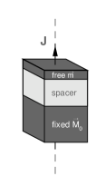
Figure 1: Spin-torque oscillator in the circuit.

The macroscopic description of this process is delivered by the Landau-Lifshitz-Gilbert-Slonczewski magnetization equation. Below, we largely follow the notation of Li_Zhou_2010 . For the unit vector $\vec{m}$ of magnetization in the free layer, the LLGS equation reads

$$\frac{d\vec{m}}{dt}=-\gamma\vec{m}\times\vec{H}_{\rm eff}+\alpha\vec{m}\times\frac{d\vec{m}}{dt}+\gamma\overline{\beta}J\,\vec{m}\times(\vec{m}\times\vec{M}_{0})$$ (1)

where the last term, as shown by Slonczewski Slonczewski , characterizes the current-driven spin transfer. Here, $\alpha$ denotes the Gilbert damping coefficient, $\gamma$ is the gyromagnetic ratio, whereas the effective Landau-Lifshitz field $\vec{H}_{\rm eff}$ consists of three components: the external magnetic field $\vec{H}_{a}$, the uniaxial anisotropy field $\vec{H}_{k}$ directed along the axis of easy magnetization, and the demagnetizing contribution $\vec{H}_{dz}$. In the spin-transfer term, $\vec{M}_{0}$ is the constant magnetization of the thick fixed layer, $\overline{\beta}$ characterizes the material properties of the free layer, and finally (but most importantly in our context), $J$ is the instantaneous current through the element. By means of this current, every oscillator is coupled to the circuit and, thereby, to the rest of the ensemble. Depending on its design, the circuit can play a role of the passive load (purely resistive circuit) or, in presence of capacitors and/or inductances, possess its own degrees of freedom. Notably, $J=J(t)$ is, in general, time-dependent: spin-transfer changes back and forth the magnetoresistance of the spin-torque oscillator (for quantitative description of this process see Grollier-Cros-Fert-06 ), therefore Eq.(1), taken out of the context of the surrounding circuit, is essentially non-autonomous.

On aligning the $x$- and $z$-axes of the coordinate system with directions of, respectively, the external field $\vec{H}_{a}$ and the demagnetization field $\vec{H}_{dz}$, Eq. (1) turns into the coupled equations for the components of $\vec{m}$:

$$\frac{1}{\Gamma}\,\frac{dm_{x}}{dt} = H_{dz}m_{y}m_{z}+\alpha\left((H_{a}+H_{k}m_{x})(m_{y}^{2}+m_{z}^{2})\right.$$ (2)

$$\left.+H_{dz}m_{x}m_{z}^{2})\right)-\overline{\beta}JM_{0}(m_{y}^{2}+m_{z}^{2})$$

$$\frac{1}{\Gamma}\,\frac{dm_{y}}{dt} = H_{dz}m_{z}(\alpha m_{y}m_{z}-m_{x})-H_{k}m_{x}(\alpha m_{x}m_{y}+m_{z})$$

$$-H_{a}(\alpha m_{x}m_{y}+m_{z})+\overline{\beta}JM_{0}(m_{x}m_{y}-\alpha m_{z})$$

$$\frac{1}{\Gamma}\,\frac{dm_{z}}{dt} = (H_{a}+H_{k}m_{x})(m_{y}-\alpha m_{x}m_{z})$$

$$-\alpha H_{dz}(m_{x}^{2}+m_{y}^{2})m_{z}+\overline{\beta}JM_{0}(m_{x}m_{z}+\alpha m_{y})$$

where $\Gamma$ abbreviates the factor $\gamma/(1+\alpha^{2})$. Choice of the coordinate system implies that the coefficients $H_{a}$ and $H_{dz}$ are positive; the value of $H_{k}$, without restrictions, can be viewed as positive as well.

2.1 States of equilibrium and their stability

Since the vector $\vec{m}$ is orthogonal to the rhs of Eq.(1), its length is conserved, while orientation can vary in time. Accordingly, the partial phase space of a single spin-torque oscillator is the two-dimensional spherical surface. For a set of $N$ such oscillators, the phase space is a direct sum of $N$ spheres, augmented by directions which correspond to independent global variables of the circuit (e.g. voltage). A look at the equations (2) shows that a magnetic moment $\vec{m}$, if set parallel to the external field $\vec{H}_{a}$, stays constant and preserves orientation: if, originally, the off-field components $m_{y}$ and $m_{z}$ vanish identically, they will not be excited, and precession of $\vec{m}$ would not arise. For a single oscillator, there are two such states of equilibrium, characterized by $m_{x}=\pm 1$. For the whole ensemble this implies that every element which, in the course of evolution, gets exactly parallel to $\vec{H}_{a}$, remains in that equilibrium position forever and does not contribute to generation of the electromagnetic field. Notably, these states of equilibrium exist independently from the circuit composition and from the value of the current $J$ through the stack of STO units: what is influenced by $J$, is their stability .

Consider, first, a single STO. There are two possibilities for the equilibrium: $\vec{m}$ is oriented either along the external field $\vec{H}_{a}$ or in the opposite direction. In the equations (2) the terms containing the current $J$ are proportional to linear and quadratic terms in $m_{y},\,m_{z}$. Therefore, linearization near the states with $m_{x}=\pm 1$ (and, hence, the stability of those states) depends only on the value of the time-independent component of $J$. The equilibrium value of $J$ is dictated by the configuration of the circuit into which the oscillators are included. Below, we will list a few exemplary circuit configurations and explicitly express the respective values of $J$ through the value of the external current $I$; however, until the end of the current section we use the symbol $J$ for parameterization of dynamics near the equilibria.

To begin with, we characterize the state with $m_{x}=1$: magnetization along the external field $\vec{H}_{a}$. The characteristic equation reads

$$\lambda^{2} +2\lambda\left(\alpha(H_{a}+H_{k}+\frac{H_{dz}}{2})-\beta J\right)$$

$$+(1+\alpha^{2})\left(\beta^{2}J^{2}+(H_{a}+H_{k})(H_{a}+H_{k}+H_{dz})\right)=0.$$

(here $\beta$ denotes the product $\overline{\beta}M_{0}$, and the factor $\Gamma$ is absorbed in the time units).

Since the last term of Eq.(2.1) is positive, two eigenvalues cannot have opposite signs. If the current $J$ is absent or sufficiently weak, the equilibrium is stable; it gets destabilized in the Hopf bifurcation at

$$J=J_{H}=\frac{\alpha}{\beta}\,(H_{a}+H_{k}+\frac{H_{dz}}{2}).$$ (4)

The second equilibrium, with magnetization directed opposite to the external field $\vec{H}_{a}$ ($m_{x}$=–1), looks intuitively unstable. This is indeed true, as long as the current $J$ is not too large. The corresponding characteristic equation is

$$\lambda^{2} +2\lambda\left(\beta J+\alpha(H_{k}-H_{a}+\frac{H_{dz}}{2})\right)$$

$$+(1+\alpha^{2})\left(\beta^{2}J^{2}+(H_{k}-H_{a})(H_{k}-H_{a}+H_{dz})\right)=0.$$

For $\displaystyle J<J_{st}=\frac{1}{\beta}\sqrt{(H_{a}-H_{k})(H_{k}-H_{a}+H_{dz})}$, the last term is negative, and the steady state is a saddle. At $J=J_{st}$ the pitchfork bifurcation stabilizes this equilibrium.

For generic values of $H_{k},\,H_{a},\,H_{dz}$ the value $J_{st}$ exceeds $J_{H}$ by the order of $1/\alpha$. Since the Gilbert damping coefficient $\alpha$ is typically of the order of $10^{-2}$ Sinova_2004 , this ensures a broad range of values of $J$ in which one equilibrium state is an unstable focus whereas another one is a saddle point, regardless of the design of the circuit into which the STO elements are serially included. Within this range of $J$, every unit in a set of identical spin-torque elements performs oscillations, and later we will show that at least in some part of the range those oscillations cannot be synchronized.

In stack of $N$ STO, each element can occupy any of two possible equilibrium positions, hence there are altogether $2^{N}$ collective states of equilibrium. Consider the configuration with $N_{+}\geq 0$ oscillators having $m_{x}=1$ and the remaining $N_{-}=N-N_{+}$ units with $m_{x}=-1$. Eigenvalues that characterize growth/decay of small deviations for the former oscillators obey Eq.(2.1); each of them is $N_{+}$-times degenerate. Eigenvalues of the oscillators with $m_{x}=-1$ are described by Eq.(2.1); their degree of degeneracy equals $N_{-}$. At $J<J_{st}$ this collective equilibrium possesses $N_{-}$ real positive Jacobian eigenvalues, at $J>J_{H}$ it possesses $2N_{+}$ complex eigenvalues with positive real parts. Therefore, collective “mixed” states with part of the oscillators aligned with the field $\vec{H}_{a}$ whereas the rest is directed strictly opposite to it (i.e. $N_{+}N_{-}>0$), are unstable at all values of the current $J$. As for the “pure” states of equilibrium, the state in which all $m_{x}$ are aligned with the field is stable (unstable) below (above) $J_{H}$; the state with all magnetization vectors antiparallel to the field is a saddle with $N$ equal positive eigenvalues for $J<J_{st}$ and becomes stable beyond $J_{st}$.

For further progress, we need to know how the value of $J$ is related to the control parameters of the setup, i.e. to the total current $I$ that flows across the circuit: that relation differs over different arrangements of the circuits. Before discussing various circuits, is is convenient to lower the order of dynamical system, using the conservation of length of the vector $\vec{m}$ and proceeding from $(m_{x},m_{y},m_{z})$ to spherical angles $\theta$ and $\varphi$: $m_{x}=\sin\theta\cos\varphi$, $m_{y}=\sin\theta\sin\varphi$, $m_{z}=\cos\theta$. In the set of $N$ spin-torque oscillators each element is characterized by its own instantaneous angles $\theta_{i}$ and $\varphi_{i}$; for the $i$-th unit, Eq.(2) becomes

$$\frac{d\theta_{i}}{dt} = (\alpha H_{a}-\beta J)\cos\theta_{i}\cos\varphi_{i}$$ (6)

$$-(H_{a}+\alpha\beta J)\sin\varphi_{i}+\alpha S_{i}-T_{i}$$

$$\sin\theta_{i}\,\frac{d\varphi_{i}}{dt} = -(\alpha H_{a}-\beta J)\sin\varphi_{i}$$

$$-(H_{a}+\alpha\beta J)\,\cos\varphi_{i}\cos\theta_{i}-S_{i}-\alpha T_{i},$$

where the symbols $S_{i}$ and $T_{i}$ denote, respectively, the combinations $(H_{dz}+H_{k}\cos^{2}\varphi_{i})\sin\theta_{i}\cos\theta_{i}$   and
$H_{k}\sin\theta_{i}\sin\varphi_{i}\cos\varphi_{i}$ Li_Zhou_2010 . Compared to (2), the time units are rescaled by the factor $\Gamma$.

The set of $N$ pairs of Eqs (6) is the main building block for all circuit configurations; particularities of circuits enter these equations as soon as $J$ is expressed through the control parameters of the circuit.

3 Circuits with serially connected STOs: equations of motion.

Interaction within the set of STOs is mediated by the time-dependent common current $J(t)$ through the stack; variations of $J(t)$ are caused by variable magnetoresistance of the units. Spin transfer changes the instantaneous resistance of the STO: decreases it, when magnetization in the free layer is aligned with the external field, and enhances it when the magnetization includes a component, directed opposite to the field. As demonstrated in Grollier-Cros-Fert-06 , the value of magnetoresistance is a harmonic function of the instantaneous angle $\phi_{\vec{m}\vec{M}_{0}}$ between the magnetizations $\vec{m}$ and $\vec{M_{0}}$, adequately represented by $\cos\phi_{\vec{m}\vec{M}_{0}}$. The lowest value of resistance, $r_{p}$, is achieved in the case when both magnetizations are parallel; the highest one, $r_{ap}$, corresponds to antiparallel magnetizations. In our configuration, $\vec{M}_{0}$ is directed along the $x$-axis, hence $\cos\phi_{\vec{m}\vec{M}_{0}}=m_{x}$. Accordingly, the resistance of the STO is

$$r(t)=\frac{r_{p}+r_{ap}}{2}\,\big{(}1-\varepsilon\,m_{x}(t)\big{)}$$

where $\varepsilon$ denotes the ratio $(r_{ap}-r_{p})/(r_{ap}+r_{p})$, so that $0<\varepsilon<1$.

Below, while treating the stacks of $N$ serially connected STOs, we assume that the units are identical: they share the values of constants $\alpha,\,\beta,\,H_{a},\,H_{k},\,H_{dz},\,\varepsilon$. Due to serial connection of the STOs, the $x$-component of magnetization is effectively averaged over the stack:

$$r(t)=\frac{r_{p}+r_{ap}}{2}\,\left(1-\varepsilon\langle m_{x}\rangle\right)$$ (7)

with

$$\langle m_{x}\rangle=\frac{1}{N}\sum_{i}^{N}\sin\theta_{i}\cos\phi_{i}.$$ (8)

In the collective state of equilibrium with individual vectors of magnetizations of all STOs directed along (or opposite to) the external field, $\langle m_{x}\rangle=1$ (respectively, $\langle m_{x}\rangle=-1$). In the mixed equilibrium state, $\langle m_{x}\rangle=2N_{+}/N-1$.

Consider three exemplary circuits with $N$ serially connected STOs where the governing parameter is the constant external current $I$: the purely resistive load, a circuit with capacitor parallel to the stack, and a circuit with the $LC$ element.

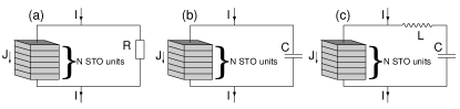
Figure 2: Serially connected STOs in exemplary circuits:
(a) resistive load, (b) RC circuit, (c) LC circuit.

3.1 Resistive load

In this configuration, sketched in the left panel of Fig. 2, an ohmic load $R$ is set parallel to the STO stack. The common current through the STOs is

$$J(t)=I\frac{R}{R+r(t)}=\frac{I}{1+\rho(1-\varepsilon\langle m_{x}\rangle)},$$ (9)

where $\langle m_{x}\rangle$ is given by (8) and $\rho$ is the ratio of resistances:

$$\rho=\frac{r_{p}+r_{ap}}{2\,R}.$$

On substituting (9) into Eq.(6), we obtain a set of 2$N$ equations

$$\frac{d\theta_{i}}{dt} = \left(\alpha H_{a}-\frac{I\,\beta}{1+\rho(1-\varepsilon\langle m_{x}\rangle)}\right)\cos\theta_{i}\cos\varphi_{i}$$

$$-\left(H_{a}+\frac{\alpha I\,\beta}{1+\rho(1-\varepsilon\langle m_{x}\rangle)}\right)\sin\varphi_{i}+\alpha S_{i}-T_{i},$$

$$\sin\theta_{i}\,\frac{d\varphi_{i}}{dt} = -\left(\alpha H_{a}-\frac{I\,\beta}{1+\rho(1-\varepsilon\langle m_{x}\rangle)}\right)\sin\varphi_{i}-S_{i}-\alpha T_{i}$$

$$-\left(H_{a}+\frac{\alpha I\,\beta}{1+\rho(1-\varepsilon\langle m_{x}\rangle)}\right)\,\cos\varphi_{i}\cos\theta_{i}$$

$$i=1,\ldots,N.$$

The resistive circuit is passive: there are no independent variables besides 2$N$ angular coordinates of the STOs. Substituting the corresponding values of $\langle m_{x}\rangle$ into (9) renders equilibrium value of the current $J$:

$$J=\frac{I}{1+\rho(1\pm\varepsilon)}$$

with the sign before $\varepsilon$ in the denominator being taken opposite to the sign of $\langle m_{x}\rangle$. By inserting this expression into Eqs (2.1,4,2.1), we relate the eigenvalues of the equilibria and the threshold $I_{H}$ of the Hopf bifurcation to the external current $I$.

3.2 Circuit with a capacitor

Introduction of a capacitor parallel to the stack (central panel of Fig. 2) raises the order of the dynamical system. In this configuration the current $J$ through the stack is related to the external current $I$ by

$$J(t)\,=\,I-C\,\Gamma\,\frac{dV}{dt}$$

with $C$ denotes the capacitance and $V$ is the voltage difference on the stack; the factor $\Gamma$ translates the derivative into the rescaled time units of Eqs(6). On combining this with $V=r(t)\,J(t)$ and introducing the dimensionless voltage $\displaystyle u=\frac{2V}{I\,(r_{p}+r_{ap})}$, equations (6) turn into

$$\frac{d\theta_{i}}{dt} = (\alpha H_{a}-\frac{\beta Iu}{(1-\varepsilon\langle m_{x}\rangle)})\cos\theta_{i}\cos\varphi_{i}$$

$$-(H_{a}+\frac{\alpha\beta Iu}{(1-\varepsilon\langle m_{x}\rangle)})\sin\varphi_{i}+\alpha S_{i}-T_{i}$$

$$\sin\theta_{i}\,\frac{d\varphi_{i}}{dt} = -(\alpha H_{a}-\frac{\beta Iu}{(1-\varepsilon\langle m_{x}\rangle)})\sin\varphi_{i}-S_{i}-\alpha T_{i}$$

$$-(H_{a}+\frac{\alpha\beta Iu}{(1-\varepsilon\langle m_{x}\rangle)})\,\cos\varphi_{i}\cos\theta_{i},$$

$$i=1,\ldots,N.$$

with additional dynamical relation

$$\frac{du}{dt} = \omega\left(1-\frac{u}{(1-\varepsilon\langle m_{x}\rangle)}\right)$$ (12)

where $\omega$ denotes the parameter combination (inverse characteristic time)

$$\omega=\frac{2(1+\alpha^{2})}{\gamma\,(r_{p}+r_{ap})\,C}.$$ (13)

Altogether, dynamics is governed by $2N+1$ equations.

Since in this circuit the segment parallel to the stack bears no ohmic resistance, for every steady state the current $J$ through the stack is the whole external current $I$. Therefore, while determining stability and eigenvalues of the equilibria, the symbol $J$ in the Eqs (2.1,4,2.1), should be substituted by $I$.

3.3 LC-circuit

Including the inductance $L$ and capacitance $C$ parallel to the stack of STOs (right panel of Fig. 2) turns the circuit equation into

$$LC\Gamma^{2}\,\frac{d^{2}V}{dt^{2}}+V=r(t)\,J(t)=r(t)\left(I-C\,\Gamma\frac{dV}{dt}\right).$$ (14)

On combining (6) with (14), we arrive at the system of $(2N+2)$ ODEs Pikovsky_2013 :

$$\frac{d\theta_{i}}{dt} = \cos\theta_{i}\cos\varphi_{i}\left(\alpha H_{a}-\beta I(1-w)\right)$$

$$-\sin\varphi_{i}\left(H_{a}+\alpha\beta I(1-w)\right)+\alpha S_{i}-T_{i}$$

$$\sin\theta_{i}\,\frac{d\varphi_{i}}{dt} = -\sin\varphi_{i}\left(\alpha H_{a}-\beta I(1-w)\right)-S_{i}-\alpha T_{i}$$

$$-\cos\varphi_{i}\cos\theta_{i}\left(H_{a}+\alpha\beta I(1-w)\right)$$

$$\frac{du}{dt} = \omega\,w$$

$$\frac{dw}{dt} = \frac{\Omega^{2}}{\omega}\,\bigg{(}(1-w)\,(1-\varepsilon\langle m_{x}\rangle)\,-u\bigg{)}$$

where the variable $u$, like above in Eq.(12), is the rescaled voltage $V$, the variable $w=\displaystyle\frac{C\,\Gamma}{I}\frac{dV}{dt}$ is the rescaled time derivative of $V$, the parameter $\omega$ is defined in (13), and the additional characteristics of the circuit is its eigenfrequency $\Omega$ (expressed in units of rescaled time):

$$\Omega=\frac{1}{\Gamma\,\sqrt{L\,C}}.$$

For this configuration, like in the previous case, $J(t)=I-C\,\Gamma\,dV/dt$, therefore $J$ in the characteristic equations (2.1,2.1) should be directly substituted by external current $I$; in particular, the threshold of the Hopf bifurcation $I_{H}$ equals to (4).

Further configurations of the circuit can be treated along the same lines: combination of Kirchhof equations that describe the circuit dynamics with a set (6) of $2N$ equations for individual oscillators.

4 From the Andronov-Hopf bifurcation to homoclinics and beyond.

In absence of the external current $I$ there is no precession of magnetic field: each STO is at the stable equilibrium with $m_{x}=+1$. For a single unit, increase of $I$ across the bifurcational value (4) leads to the onset of periodic oscillations. In all three exemplary setups the same bifurcation scenario takes place: when the current $I$ is increased, the oscillation grows in amplitude and undergoes the homoclinic bifurcation at which it becomes bi-asymptotic to the saddle equilibrium with $m_{x}=-1$. Due to the symmetry of the governing equation (2) with respect to simultaneous change of sign of the off-field components $m_{y}$ and $m_{z}$, homoclinic orbits exist in pairs, therefore a periodic solution does not disappear at homoclinics; instead, periodic states recombine in the course of the so-called “gluing bifurcation” gluing . Transformation of the attracting trajectory in that bifurcation is sketched in Fig. 3.

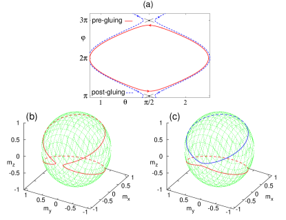
Figure 3: Recombination of attracting orbits in the gluing bifurcation. Shape of attracting trajectories in the plane (a) and spherical (b,c) projections. Dashed curves: orbit segments on the reverse side of the sphere. (b) unique limit cycle before the gluing; (c) two symmetric limit cycles after the gluing.

Divergence of period $T$ at the bifurcational parameter value $I_{\rm hom}$, shown in Fig. 4, follows the logarithmic law: $T~{}\sim-\log|I-I_{\rm hom}|$. The prefactors on different sides from $I_{\rm hom}$ differ due to the change of the orbit shape at the bifurcation our_gluing : As seen in the panels (b) and (c) of Fig. 3, the cycle of oscillation below $I_{\rm hom}$ is unique and includes two passages near the saddle point. In contrast, beyond the critical value there are two symmetric orbits, each of them containing just one passage near the saddle per rotation period.

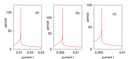
Figure 4: Period of oscillations for an individual STO: (a) resistive load, (b) RC circuit, (c) LC circuit. Common parameter values: $H_{dz}=1.6,H_{k}=0.05,H_{a}=0.2$, $\alpha$=0.01, $\beta$=10/3, $\varepsilon$=0.3. Resistive: $\rho$=1; RC and LC: $\omega$=1; LC: $\Omega=1.5$.

For an isolated STO, the periodic orbit is stable throughout the whole parameter range of its existence. For an ensemble of STOs, the synchronous periodic state in which all units share the instantaneous values of $\theta$ and $\varphi$, is obviously a solution as well; however, it may be unstable with respect to perturbations that disturb the coincidence of coordinates in the oscillating cluster. In this situation, stability of the periodic state can be characterized in terms of the so-called “evaporation multiplier” $\mu_{\rm e}$ that characterizes stability of the synchronous cluster against “evaporation” of its constituents, by quantifying within a period of oscillations the growth factor of the distance between the cluster and an infinitesimally displaced unit evaporation . The value of $\mu_{\rm e}$ is recovered from the solution on the time interval $(0,T)$ of the equation in normal variations near the synchronous trajectory; in those linearized equations, the contribution of perturbed unit into the global field is neglected. Within this setup, $\mu_{\rm e}$ is the leading multiplier of the monodromy matrix (in our case, with each unit having two coordinates $\theta_{i}$ and $\varphi_{i}$, this is a $2\times 2$ matrix). If $|\mu_{\rm e}|<1$, the cluster is stable with respect to splitting .

Numerically recovered dependence $\mu_{\rm e}(I)$ for exemplary configurations is plotted in Fig. 5. The common feature for all circuits is apparent strong divergence of $\mu_{\rm e}(I)$ at $I=I_{\rm hom}$. Otherwise, stability differs for different setups. For the resistive load (curve in Fig.5a) the oscillating cluster becomes unstable with respect to splitting immediately after its birth in the Andronov-Hopf bifurcation (recall that for a solitary unit the periodic orbit stays asymptotically stable); divergence at $I=I_{\rm hom}$ is followed by the parameter interval in which $\mu_{\rm e}$ is negative, and, somewhat later, by stabilization of synchrony (the multiplier enters the unit circle at $\mu_{\rm e}=-1$). The clusters in RC and LC contours, in contrast, are stable near the birth of the periodic solution, lose stability shortly before the homoclinic bifurcation and remain (weakly) unstable for all values of $I$ beyond the bifurcation. The most remarkable effect is the extremely sharp growth of $\mu_{\rm e}(I)$ for periodic solutions close to homoclinicity; there, the distance in the phase space between the cluster and the detached unit grows by many orders of magnitude within a single turn in the phase space. This effectively prohibits existence of stable synchronous oscillations in the adjacent parameter range.

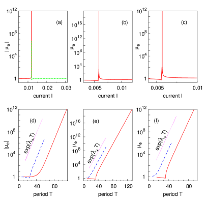
Figure 5: Evaporation multiplier for the synchronous periodic oscillation. Left column (a,d): resistive load, middle column (b,e): RC circuit, right column (c,f): LC circuit. Parameter values: see Fig. 4. In the panel (a) the dashed part of the curve (to the right from the peak) corresponds to negative values of $\mu_{\rm e}$. In the bottom row, solid and dashed curves correspond, respectively, to the current ranges below $I_{\rm hom}$ and above $I_{\rm hom}$; dotted straight lines show plots of $\exp(\lambda_{+}T)$.

The singularity of the evaporation multiplier at homoclinicity is enrooted in the divergence of period. Consider linearization of the flow near the synchronous time-dependent trajectory. To compute $\mu_{\rm e}$, the initial disturbance $x(0)$ should be set on the appropriate eigenvector of the monodromy matrix; then $\log\mu_{\rm e}$=$\log\big{(}\|x(T)\|/\|x(0)\|\big{)}$ $\approx\int_{0}^{T}\lambda(t)dt$ where $\lambda(t)$ is the leading eigenvalue of the instantaneous Jacobian matrix. Near homoclinicity, the system spends the prevalent proportion of time in the very slow motion across the vicinity of the saddle point where $\lambda(t)$ is virtually indistinguishable from the positive eigenvalue $\lambda_{+}$ at the saddle: the larger root of Eq.(2.1). Therefore the integral (and with it, the evaporation multiplier) is dominated by $\exp(\lambda_{+}T)$. In Fig. 5 where the evaporation multiplier is plotted versus the period of the orbit, the dependence $\mu_{\rm e}\sim\exp(\lambda_{+}T)$ is doubtless. Notably, the prefactor before the exponent at the pre-homoclinic branch is the squared prefactor at the post-homoclinic branch (cf. its double distance from the dotted line in the logarithmic vertical scale of the bottom plots); this owes to the fact that the periodic orbit traverses the region, non-adjacent to the saddle, twice below $I_{\rm hom}$ but once above $I_{\rm hom}$.

The exponential growth of the evaporation multiplier near homoclinicity is generic: at the critical parameter value, local dynamics near the synchronous limit cycle occurs in the subspace that is tangential to the plane in which the equilibrium, participating in the homoclinic bifurcation, has its local unstable manifold. During the long epoch in which the motion is directed along that manifold, generic distances grow as $\exp({\lambda_{+}t})$. The same arguments should ensure the instability of synchronous nearly homoclinic one-cluster oscillation in every other setup with generic global coupling of units.

In the situations that lack the symmetries ensuring the gluing of periodic orbits at the saddle point, the “usual” homoclinic bifurcation takes place, with periodic state existing only on one side of the bifurcation parameter value. In accordance with the above reasoning, this collective periodic solution should lose stability with respect to splitting of the synchronous cluster well before the homoclinicity.

Remarkably, destabilization of synchronous states close to homoclinic trajectories has a counterpart in the dynamics of distributed systems. In many translationally invariant spatial systems governed by partial differential equations, evolution of spatially homogeneous solutions is finite-dimensional. Certain types of attractors for such finite-dimensional dynamics, including the homoclinic trajectories and temporally periodic solutions close to homoclinic orbits, were shown to be generically unstable with respect to spatial perturbations in the form of longwave modulation Coullet_Riesler_2000 ; Riesler_2001 . The situation discussed in the present manuscript is reminiscent of that effect: here, the ensemble of finite size replaces the continuum that is present in the PDE context. In both cases, the uniform (synchronous) dynamics is described by a low-dimensional set of equations that in appropriate parameter ranges possess attracting periodic solutions close to the homoclinic trajectories, and in both cases these regimes yield to perturbations that disturb the uniformity.

Numerical experiments with the STO ensembles beyond the threshold values of constant current $I$ in different circuit configurations disclose, mostly, complicated dynamical states with various degrees of asynchrony Pikovsky_2013 ; sci_rep_2017 ; in Fig. 6 we exemplify a few of them by projecting all magnetization vectors onto the same spherical surface. Within this representation, in the course of temporal evolution the instantaneous states of the units typically move along narrow ring-shape bands.

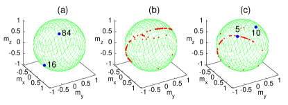
Figure 6: Snapshots of collective states in the LC circuit with $N$=100 STOs. Filled red circles: positions of individual oscillators. Filled blue circles: clusters of oscillators (numbers indicate respective populations.) (a) periodic state with two clusters; (b) disperse state where all STOs are disjoint; (c) chimera-like state, combining clusters with isolated oscillators.

5 Action of common noise

From the point of view of applications, a reasonable way to interfere into dynamics is to introduce temporal variations for the external current $I$. Since the same $I(t)$ is perceived by all STO units, it can be viewed as a common time-dependent signal which affects the whole ensemble. Below we restrict ourselves to the case of modulation with white Gaussian noise: $I(t)=I_{0}\left(1+\sqrt{2D}\,\xi(t)\right)$; in this parameterization, $I_{0}$ renders the time-average value of the current, whereas $D$ is the intensity of the $\delta$-correlated Gaussian random variable $\xi(t)$.

5.1 Governing equations

5.1.1 Resistive case

We begin with the stack of STO with resistive load.

On substituting the expression for the modulated current into Eq.(3.1), we arrive at the set

$$\frac{d\theta_{i}}{dt} = \left(\alpha H_{a}-\frac{\beta I_{0}(1+\sqrt{2D}\,\xi(t))}{1+\rho(1-\varepsilon\langle m_{x}\rangle)}\right)\cos\theta_{i}\cos\varphi_{i}$$

$$-\left(H_{a}+\frac{\alpha\beta I_{0}(1+\sqrt{2D}\,\xi(t))}{1+\rho(1-\varepsilon\langle m_{x}\rangle)}\right)\sin\varphi_{i}+\alpha S_{i}-T_{i},$$

$$\sin\theta_{i}\,\frac{d\varphi_{i}}{dt} = -\left(\alpha H_{a}-\frac{\beta I_{0}(1+\sqrt{2D}\,\xi(t))}{1+\rho(1-\varepsilon\langle m_{x}\rangle)}\right)\sin\varphi_{i}-S_{i}-\alpha T_{i}$$

$$-\left(H_{a}+\frac{\alpha\beta I_{0}(1+\sqrt{2D}\,\xi(t))}{1+\rho(1-\varepsilon\langle m_{x}\rangle)}\right)\,\cos\varphi_{i}\cos\theta_{i},$$

$$i=1,\ldots,N.$$

The random variable $\xi(t)$ enters these equations at 4$N$ places, assuming the same value in all of them.

5.1.2 STO stack with CR circuit

In the circuit with the capacitor, introduction of the modulation of the current does not change the $2N$ governing equations (3.2) for $N$ individual spin-torque oscillators (up to replacing the symbol $I$ by constant $I_{0}$). The only modification concerns the equation for the voltage (12) which now reads

$$\frac{du}{dt} = \omega\left(1+\sqrt{2D}\,\xi(t)-\frac{u}{(1-\varepsilon\langle m_{x}\rangle)}\right)$$ (17)

with $D$, like above, being the intensity of the Gaussian white noise $\xi(t)$. Accordingly, the common noise directly influences dynamics only via the global variable $u$.

5.1.3 STO stack with LC circuit

For time-dependent current $I\left(1+\sqrt{2D}\xi(t)\right)$, the ensemble is governed by equations

$$\frac{d\theta_{i}}{dt} = U(t)\,\cos\theta_{i}\cos\varphi_{i}-W(t)\,\sin\varphi_{i}+\alpha S_{i}-T_{i}$$

$$\sin\theta_{i}\,\frac{d\varphi_{i}}{dt} = -U(t)\,\sin\varphi_{i}-W(t)\,\cos\varphi_{i}\cos\theta_{i}-S_{i}-\alpha T_{i}$$

$$\frac{du}{dt} = \omega\,w$$ (18)

$$\frac{dw}{dt} = \frac{\Omega^{2}}{\omega}\,\bigg{(}(1+\sqrt{2D}\xi(t)-w)$$

$$\hskip 19.91684pt(1-\frac{\varepsilon}{N}\sum_{j}\sin\theta_{j}\cos\varphi_{j})-u\bigg{)}$$

with explicit functions of time

$$U(t) = \alpha H_{a}-\beta(1-w)I_{0}\left(1+\sqrt{2D}\xi(t)\right),$$

$$W(t) = H_{a}+\alpha(1-w)\beta I_{0}\left(1+\sqrt{2D}\xi(t)\right).$$

Thereby, in the system of equations the same value of the random variable $\xi$ is employed at $4N+1$ places.

5.2 Collective dynamics in presence of common noise: phenomenology.

Ensemble dynamics, recovered at $D>0$ by numerical integration of the stochastic equations of motion for $N$=100 and $N$=200 STOs at the values of average current beyond the threshold of the Hopf bifurcation, reminds, in most of the cases, disperse states in the deterministic setup. Neither durable states with synchronous oscillations of all or, at least, of the bulk of the elements, nor persistent clusters were observed. In all studied types of circuits, simulations at low values of $D$ feature asynchronous dynamics of individual STOs; instantaneous states of magnetization vectors form bands on the surface of the unit sphere; when the noise intensity is raised, the bands become wider, and now and then separate units temporarily leave the bands, performing large excursions over the sphere. This behavior seems to be largely insensitive to the initial conditions: the same kind of dynamical states evolves from the narrow distributions near particular points of the sphere and from random homogeneous scattering over the spherical surface.

5.2.1 Serial stacks of STO with resistive and RC load: intermittent alignment with the external field at high intensity of common noise.

At very large amplitudes of noise, $D\gg 1$, temporal evolution in the stacks with purely resistive load and with the RC load displays a certain kind of intermittency. From time to time, all magnetization vectors align themselves to the permanent external field; on the surface of the sphere this is seen as temporary contraction of the ensemble to the equilibrium point with $m_{x}$=1. In the plots of $m_{x}(t)$ (Fig. 7), these stages are represented by horizontal plateaus.

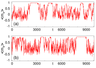
Figure 7: Intermittent alignment to the external magnetic field at high intensities of common noise. $I_{0}=0.01,D=40$.
(a) Circuit with purely resistive load, $\rho$=1. (b) Circuit with RC load, $\omega$=1. Other parameter values: see Fig. 4.

Recall that in this range of values of the average current, the state of magnetization along the external field is unstable. The plateaus at $m_{x}$=1 owe to repetitive macroscopic segments of time in which the local running average over $\xi(t)$ is sufficiently negative, so that the real parts of the instantaneous leading Jacobian eigenvalues at the steady state are temporarily driven deep into the negative domain. This ensures short-term sustainment of the unstable equilibrium.

5.2.2 Serial stacks of STO with LC load: ensemble contracts to a point.

In the case of the STO stack included into the LC circuit, alignment with the external field becomes permanent. In the range of moderate noise values, magnetic moments of all STOs, regardless of the ensemble size and of their initial orientation, gradually converge to the state with $m_{x}$=1: all of them become parallel to the external magnetic field. For the ensemble of 100 STO units, subsequent stages of the evolution on the unit sphere are shown in Fig. 8.

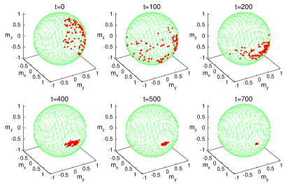
Figure 8: Snapshots of collective states in the LC circuit with $N$=100 STOs at different time values. Filled red circles: positions of individual oscillators.

Instantaneous individual magnetizations, initially randomly scattered over large areas of the sphere, gradually evolve into the broad fuzzy (and non-uniformly populated) ring-shaped band revolving around the equilibrium configuration $m_{x}=1$; as time goes on, the band contracts and finally shrinks to a point. Convergence to $m_{x}$=1 implies gradual vanishing of the off-field components $m_{y}$ and $m_{z}$. To visualize this process, we plot in the left panel of Fig. 9 temporal dependencies for the averaged values $\langle m_{y}\rangle$ and $\langle m_{z}\rangle$.

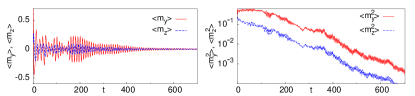
Figure 9: Temporal evolution of the mean off-field components at $I=0.01,D=0.5$ with $N$=100. Other parameter values: see Fig. 4(c).

In the course of time, irregular evolution of off-field averages is replaced by ordered oscillatory decay. Since smallness of $\langle m_{y}\rangle$ and $\langle m_{z}\rangle$ does not exclude ring-like configurations of units, we present in the right panel of Fig. 9 the evolution of mean squared characteristics $\langle m_{y}^{2}\rangle$ and $\langle m_{z}^{2}\rangle$.

In the deterministic setup this range of the current $I$ corresponds to the unstable collective equilibrium with $m_{x}$=1 and to angular precession of the magnetic moment. We see that in the LC configuration of the circuit the action of sufficiently strong common noise is able to stabilize the equilibrium and to suppress precession completely.  Notably, this phenomenon bears the threshold character: for it to occur, the intensity of noise should exceed the certain level.

5.3 Collective dynamics in presence of common noise: local analysis.

Since the same noise acts upon all identical units, the system of stochastic equations admits a synchronous solution in which the instantaneous values of all $\theta_{i}$ as well as of all $\varphi_{i}$ coincide. Stability of this solution is characterized in terms of the transversal Lyapunov exponent: the average growth rate of disturbances, splitting the synchronous dynamics. Below we study dependence of this characteristics on the average current $I_{0}$ and noise intensity $G$ for all considered types of STO circuits.

5.3.1 STO with resistive and RC load: absence of noise-induced large-scale stabilization

We start with the purely resistive circuit. Dependence of the transversal Lyapunov exponent on $I_{0}$ and $D$ is shown in Fig. 10.

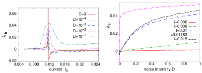
Figure 10: Circuit with purely resistive load under noisy currrent. Transversal Lyapunov exponent as a function of average current $I_{0}$ at fixed noise intensity $D$ (left panel) and as a function of $D$ at fixed $I_{0}$ (right panel). Parameter values: see Fig. 4a).

Recall that in the deterministic case $D$=0, the evaporation multiplier $\mu_{\mbox{e}}$ of the periodic solution diverges at the value of $I$ corresponding to homoclinicity. As a consequence, the transverse Lyapunov exponent $\lambda_{\mbox{tr}}$, that for a closed orbit with period $T$ equals $\log(|\mu_{\mbox{e}}|)/T$, tends to the largest eigenvalue of the Jacobian matrix at the equilibrium. In presence of noise, the system spends less time in the vicinity of the equilibrium where the instability rates are especially high; this results in broadening and softening of the peak in the dependence of $\lambda_{\mbox{tr}}$ on $I_{0}$. This tendency is apparent in the left panel of Fig. 10: the higher the noise intensity $D$, the broader the maximum of $\lambda_{\mbox{tr}}$. Over large intervals of $I_{0}$ the weak noise shifts $\lambda_{\mbox{tr}}$ downwards; this results in ranges of $I_{0}$ with mildly negative transversal Lyapunov exponent. The effect, however, remains local in the phase space and does not seem to influence global dynamics of the STO ensembles: as already mentioned, unless the initial distribution of oscillators in the ensemble is extremely narrow, simulations show no convergence to the synchronous 1-cluster solution. The stronger noise, exemplified in Fig. 10 by the curve for $D=10^{-1}$, raises the value of $\lambda_{\mbox{tr}}$ everywhere outside the immediate vicinity of the homoclinic singularity, and amplifies the instability of the synchronous state. In the right panel the same transversal Lyapunov exponent is plotted as a function of noise intensity at several fixed values of the average current $I_{0}$; except the narrow region adjoining the deterministic case, $\lambda_{\mbox{tr}}$ appears to be a roughly monotonically growing function of $D$.

Proceeding to the case of the STO stack with the RC load (Fig. 11), we observe that here, as well, introduction of the noisy modulation of the common current broadens and softens the peak of the transversal Lyapunov exponent, rendering $\lambda_{\mbox{tr}}$, over the large parameter ranges, positive. Summarizing, in neither of these two circuit configurations does the common noise facilitate synchrony.

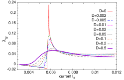
Figure 11: Circuit with the RC load. Dependence of transversal Lyapunov exponent on the average current $I_{0}$ at different intensities $D$ of common noise. Parameter values: see Fig. 4b)

5.3.2 STO in the LC circuit: noise-induced oscillation death

The situation in presence of the LC load is qualitatively different from the discussed cases.

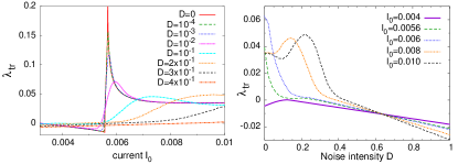
Figure 12: STO in a circuit with LC load and common noise. Transversal Lyapunov exponent as a function of current $I_{0}$ at fixed noise intensity $D$ (left panel) and as a function of noise intensity $D$ at fixed current $I_{0}$ (right panel). Parameter values: see Fig. 4c)

Fig. 12 shows the values of the transversal Lyapunov exponent computed for different combinations of the average current $I_{0}$ and noise intensity $D$. As seen in the left panel, like in the previously discussed cases, the action of noise softens and widens the maximum of the transversal Lyapunov exponent. There is, however, an apparent difference: the maximum not only becomes broader, but, in contrast to the cases of resistive load or the circuit with a capacitor, it gets shifted from the place of homoclinic bifurcation in the deterministic system towards higher values of $I_{0}$. At sufficiently large noise intensity $D$, the transversal exponent $\lambda_{\mbox{tr}}$ stays negative in the broad range of $I_{0}$. The right panel of Fig. 12 presents the same results from the different perspective; variation of noise intensity at several fixed values of $I_{0}$. In the right half of the plotted range of $D$, the dependence of $\lambda_{\mbox{tr}}$ on $D$ becomes virtually linear, with negative slope. Remarkably, within numerical accuracy all curves $\lambda_{\mbox{tr}}(D)$ intersect in the same point.

Recall that for moderate intensity of noise (in the right panel of Fig. 12 this corresponds to $D>0.4$) simulations of ensemble of noise-driven STOs in the LC circuit have demonstrated trapping of all oscillators by the equilibrium state. In the context in which all trajectories eventually end up at the equilibrium, the Lyapunov exponents turn into the real parts of the eigenvalues of the Jacobian at that equilibrium. The real part of two leading eigenvalues equals

$$\lambda = -\alpha\left(H_{a}+H_{k}+\frac{H_{dz}}{2}\right)+\beta\,\overline{(1-w(t))I(t)}$$

$$= -\alpha\left(H_{a}+H_{k}+\frac{H_{dz}}{2}\right)+\beta\,I_{0}\,\overline{\xi(t)w(t)}\sqrt{2D}$$

where the stochastic variable $w(t)$ (the rescaled time derivative of the voltage $u$), is governed by the last of Eq. (5.1.3), and the overline denotes averaging over time.

To estimate $\overline{\xi(t)w(t)}$ we utilize the fact that the equilibrium value of $u$ equals $1-\varepsilon$ and assume that near the equilibrium the variable $w(t)$ obeys the Gaussian distribution centered at zero. In this way we derive

$$\overline{\xi(t)w(t)}=\frac{\Omega^{2}(1-\varepsilon)}{2\omega}\sqrt{2D}$$

and, finally, arrive at

$$\lambda = \beta(I_{0}-I_{H})-\frac{\Omega^{2}(1-\varepsilon)\beta\,I_{0}}{\omega}\,D$$

$$= \beta\left(I_{0}-\frac{\alpha}{\beta}(H_{k}+H_{a}+\frac{H_{dz}}{2})\right)-\frac{\Omega^{2}(1-\varepsilon)\beta\,I_{0}}{\omega}\,D.$$

Notably, this expression involves, without exception, all parameters of the stochastic differential equations (5.1.3). The last term (recall that $\varepsilon<1$ by definition) shows that the noise always lowers the value of $\lambda$.

For $I_{0}>I_{H}$, the Lyapunov exponent of the equilibrium in the absence of noise is positive. Stochastic trajectories only seldom (if at all) visit the neighborhood of the equilibrium, therefore the value of this exponent stays local, dynamically irrelevant and is not related to the actually observed value of the leading Lyapunov exponent for generic non-stationary trajectories. Increase of the noise intensity weakens the instability, leading to the gradual decline of $\lambda$. Finally, on crossing the critical value

$$D_{\rm trap}=\,\frac{\omega}{\Omega^{2}(1-\varepsilon)}\left(1-\frac{I_{H}}{I_{0}}\right)$$ (20)

the equilibrium gets stabilized and turns into the global attractor. Henceforth, linearization in its vicinity dominates also the global Lyapunov exponent and becomes well visible at its plots. Remarkably, the value of $D_{\rm trap}$ is a monotonically growing bounded function of the average current $I_{0}$: noise with intensity $\displaystyle D>D_{g}=\frac{\omega}{\Omega^{2}(1-\varepsilon)}$ guarantees trapping of all oscillators at arbitrary values of the current (under employed values of the circuit parameters, $D_{g}\approx 0.635$).

The estimate (5.3.2) turns out to be rather accurate: in all our simulations for $D>D_{\rm trap}$, the relative discrepancy between the theoretical prediction (5.3.2) and numerically computed value of the Lyapunov exponent of the stochastic trajectory never exceeded 0.8%.

Linear dependence on the noise intensity $D$ explains both the linear character of the curves in the right part of Fig. 12 and the fact of intersection of all curves in the right panel of Fig. 12 in the same point.

On the parameter plane spanned by the average current $I_{0}$ and the noise intensity $D$ the region of trapping, adjoining the region in which the equilibrium is stable, lies to the right from $I_{\rm hopf}$ (Fig. 13); its lower boundary branches from zero and grows in the direction of $D_{g}$ at larger values of $I_{0}$.

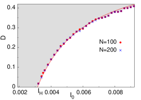
Figure 13: Stabilization border for $N$=100 and $N$=200. Solid line: theoretical prediction (20). Crosses and circles: numerically determined threshold values of $D$ for the ensembles of, respectively, 100 and 200 STOs. Gray background: region of stability for the equilibrium with $m_{x}$=1

.

Notably, this stabilization of the equilibrium by common noise with subsequent trapping of the ensemble can hardly be called a collective phenomenon: the ensemble size $N$ enters neither Eq. (5.3.2) for the Lyapunov exponent nor the expression (20) for the critical noise intensity. A single spin-torque rotator in the LCR circuit with $I_{0}>I_{\rm H}$ would be attracted to the equilibrium $m_{x}$=1 as well, provided that the noise intensity $D$ exceeds the threshold (20). Numerically, we estimated the threshold for ensembles of different sizes, by maximizing over hundreds of realizations the values of $D$ at which macroscopic parts of the ensemble were still not trapped after $t=10^{5}$. These critical values display practically no variation when the ensemble size is doubled (cf. crosses and circles in Fig. 13. Only the relaxation time, required for trapping of the last ensemble element shows a slight increase for the larger $N$. A single spin-torque rotator in the LC circuit with $I_{0}>I_{\rm H}$ would be attracted to the equilibrium $m_{x}$=1 whenever the noise intensity $D$ exceeds the threshold (20).

5.4 Discussion

A natural question is: why does the LC circuit under common noise enable complete trapping of the ensemble whereas the other configurations of the circuit fail to feature durable stabilization of the equilibrium? The explanation is given by the way in which the individual and the collective (if present) variables are affected by the common noise. In the circuit with purely resistive load, governing equations for the angular variables explicitly include the random term $\xi(t)$. Although the instantaneous value of the leading equilibrium eigenvalue contains terms proportional to $\xi(t)$, in the long run these terms average out and bear no influence on the overall value $\lambda$ of the Lyapunov exponent (although, as we have seen, within finite time windows this value can stay negative, featuring a kind of intermittent stabilization). In contrast, equations for the angular variables in the stochastic circuit with the capacitor do not contain random terms; there, noise is explicitly present only in the governing equation for the global (collective) variable $u$ (rescaled voltage). This presence, as well, adds the term $\sim\xi(t)$ to the expression for the instantaneous eigenvalue, but this term again averages out and does not influence $\lambda$. Finally, dynamical description of the circuit with the LC load involves noisy terms both in the angular variables and in one of the global variables. As a result, the expression for the instantaneous leading eigenvalue of the Jacobian (cf. Eq.(5.3.2)) contains the product of two random terms, and the non-zero average value of this product serves for the systematic noise-induced shift of $\lambda$.

6 Conclusion

The main goal of this paper was to focus on peculiarities of the STOs that strongly affect their synchronization properties. We show that the gluing bifurcation implies divergence of the transversal Floquet multiplier, responsible for stability of the synchronized cluster. This phenomenon is intrinsic to the STO dynamics and cannot be mitigated by variations of the load; the only way to avoid the instability appears to select external control parameters to be far away of the homoclinic transition. We also analyzed another important factor influencing the dynamics of STOs, namely fluctuations of the current through the array. Here we observed a novel feature of suppression of oscillations, which can be interpreted as noise-induced oscillation death. Here a distribution of the external noisy input between the stack of STOs and the parallel load is important: only an LC load leads to an effective shift of the Hopf bifurcation end eventual stabilization of the steady state by noise.

Acknowledgments
Numerical part of this work conducted by A.P. was supported by the Russian Science Foundation (Project No. 17-12-01534). M.Z. was supported by DFG (grant PI 220/17-1).

References

- (1) Kuramoto, Y., Self-entrainment of a population of coupled nonlinear oscillators, In Araki, H. (ed.), International Symposium on Mathematical Problems in Theoretical Physics, Springer Lecture Notes Phys., v.39, p.420, New York, (1975).
- (2) S. Gupta, A. Campa and S. Ruffo, Statistical Physics of Synchronization, Springer (2018).
- (3) Pikovsky, A. and Rosenblum, M., Chaos 25, 097616 (2015).
- (4) Slavin, A., Tiberkevich, V. IEEE T. Magn. 45, 1875 (2009).
- (5) Chen, T. et al. Proceedings of the IEEE 104, 1919 (2016).
- (6) Abreu Araujo, F., Grollier, J. Journal of Applied Physics 120, 103903 (2016).
- (7) H.-H. Chen, C.-M. Lee, Z. Zhang, Y. Liu, J.-C. Wu, L. Horng, C.-R. Chang Phys. Rev. B 93, 224410 (2016).
- (8) Yogendra, K., Fan, D., Roy, K. IEEE Transactions on Magnetics 51, 4003909 (2015).
- (9) F. Abreu Araujo, A. D. Belanovsky, P. N. Skirdkov, K. A. Zvezdin, A. K. Zvezdin, N. Locatelli, R. Lebrun, J. Grollier, V. Cros, G. de Loubens, O. Klein. Phys. Rev. B 92, 045419 (2015).
- (10) Kendziorczyk, T., Demokritov, S. O., Kuhn, T. Phys. Rev. B 90, 054414 (2014).
- (11) V. E. Demidov, H. Ulrichs, S. V. Gurevich, S. O. Demokritov, V. S. Tiberkevich, A. N. Slavin, A. Zholud, S. Urazhdin, Nature Communications 5, 3179 (2014).
- (12) S. Erokhin and D. Berkov, Phys. Rev. B 89, 144421 (2014).
- (13) R. Lebrun, A. Jenkins, A. Dussaux, N. Locatelli, S. Tsunegi, E. Grimaldi, H. Kubota, P. Bortolotti, K. Yakushiji, J. Grollier, A. Fukushima, S. Yuasa, and V. Cros Phys. Rev. Lett. 115, 017201 (2015).
- (14) V. Flovik, F. Maciá, and E. Wahlström, Sci. Rep. 6, 32528 (2016).
- (15) Grollier, J., Cros, V., Fert, A. Phys. Rev. B 73, 060409(R) (2006).
- (16) Georges, B., Grollier, J., Cros, V., Fert, A. Appl. Phys. Lett. 92, 232504 (2008).
- (17) D. Li, Y. Zhou, C. Zhou, and B. Hu, Phys. Rev. B 82, 140407(R) (2010).
- (18) Li, D., Zhou, Y., Hu, B., Zhou, C. Phys. Rev. B 84, 104414 (2011).
- (19) Li, D., Zhou, Y., Hu, B., Åkerman, J., Zhou, C. Phys. Rev. B 86, 014418 (2012).
- (20) Pikovsky, A., Phys. Rev. E 88, 032812 (2013).
- (21) J. Turtle, P.-L. Buono, A. Palacios, C. Dabrowski, V. In, and P. Longhini, Phys. Rev. B, 95, 144412 (2017).
- (22) V. Tiberkevich, A. Slavin, E. Bankowski and G. Gerhart, Appl. Phys. Lett. 95, 262505 (2009).
- (23) S. Tsunegi, T. Taniguchi, R. Lebrun, K. Yakushiji, V. Cros, J. Grollier, A. Fukushima, S. Yuasa and H. Kubota, Sci. Rep. 8, 13475 (2018).
- (24) M. Zaks, A. Pikovsky, Scientific Reports 7, 4648 (2017).
- (25) B. Subash, V. K. Chandrasekar, and M. Lakshmanan, EPL 109, 17009 (2015).
- (26) R. Lebrun, S. Tsunegi, P. Bortolotti, H. Kubota, A.S. Jenkins, M. Romera, K. Yakushiji, A. Fukushima, J. Grollier, S. Yuasa and V. Cros, Nat. Com. 8, 15825 (2017).
- (27) J. Turtle, K. Beauvais, R. Shaffer, A. Palacios, V. In, T. Emery, and P. Longhini, J. Appl. Phys., 113, 114901 (2013).
- (28) M. A. Zaks, A. Pikovsky, Physica D 335, 33 (2016).
- (29) K. Nakada, S. Yakata and T. Kimura J. Appl. Phys. 111, 07C920 (2012).
- (30) H. Arai and H. Imamura, IEEE Transactions on Magnetics 53, 6100705 (2017).
- (31) J. C. Slonczewski, J. Magn. Magn. Mater. 159, L1 (1996).
- (32) J. Sinova, T. Jungwirth, X. Liu, Y. Sasaki, J. K. Furdyna, W. A. Atkinson, and A. H. MacDonald, Phys. Rev. B 69, 085209 (2004).
- (33) J. M. Gambaudo, P. Glendinning and C. Tresser, Nonlinearity 1, 203 (1988).
- (34) A. Pikovsky, and A. Politi, Lyapunov Exponents. A Tool to Explore Complex Dynamics (Cambridge University Press, Cambridge, 2016).
- (35) P. Coullet, E. Riesler and N. Vandenberghe, J. Stat. Phys. 101, 521 (2000).
- (36) E. Riesler, Commun. Math. Phys. 216, 325 (2001).