A Center Manifold Reduction Technique
for a System of Randomly Coupled Oscillators

Abstract

In dynamical systems theory, a fixed point of the dynamics is called nonhyperbolic if the linearization of the system around the fixed point has at least one eigenvalue with zero real part. The center manifold existence theorem guarantees the local existence of an invariant subspace of the dynamics, known as a center manifold, around such nonhyperbolic fixed points. A growing number of theoretical and experimental studies suggest that some neural systems utilize nonhyperbolic fixed points and corresponding center manifolds to display complex, nonlinear dynamics and to flexibly adapt to wide-ranging sensory input parameters. In this paper, we present a technique to study the statistical properties of high-dimensional, nonhyperbolic dynamical systems with random connectivity and examine which statistical properties determine both the shape of the center manifold and the corresponding reduced dynamics on it. This technique also gives us constraints on the family of center manifold models that could arise from a large-scale random network. We demonstrate this approach on an example network of randomly coupled damped oscillators.

I Introduction

The manifold hypothesis proposes that phenomena in the physical world often lie close to a lower dimensional manifold embedded in the full high-dimensional space Géron (2017). As technological advancements have allowed the collection of large and often complex data sets, the manifold hypothesis has spurred the creation of a number of manifold learning, or manifold reduction, techniques Belkin (2003); Carlsson (2009); Genovese (2012); Dasgupta (2008); Hastie (1989); Kambhatla (1994); Kégl (2000); Narayanan (2009); Niyogi (2008); Perrault-Jones (2012); Roweis (2000); Smola (2001); Tenenbaum (2000); Weinberger (2006). In this era of “Big Data”, dimensionality reduction techniques are often part of the initial step in the data processing pipeline. Reducing dimensions can speed up model fitting, aid in visualization, and avoid the pitfalls of overfitting in high-dimensional data sets Géron (2017).

In the field of neuroscience, where large collections of high-dimensional data are often the focus of research, a growing number of studies suggest that neural systems lie close to a dynamical systems structure known as a center manifold. These studies include entire hemisphere ECoG recordings Solovey (2012); Alonso (2014); Solovey (2015), experimental studies in premotor and motor cortex Churchland (2012), theoretical Seung (1998) and experimental studies Seung (2000) of slow manifolds (a specific case of center manifolds) in oculomotor control, slow manifolds in decision making Machens (2005), Hopf bifurcation Poincarè (1893); Hopf (1942); Andronov in the olfactory system Freeman (2005) and cochlea Choe (1998); Eguíluz (2000); Camalet (2000); Kern (2003); Duke (2003); Magnasco (2003); Hayton 2018b , a nonhyperbolic model of primary visual cortex Hayton 2018a , and theoretical work on regulated criticality Bienenstock (1998).

To understand center manifolds, we now review some basic ideas and definitions from dynamical systems theory. First, the classical approach to studying behavior in the neighborhood of an equilibrium point is to examine the eigenvalues of the Jacobian of the system at this point. If all eigenvalues have nonzero real part, then the equilibrium point is called hyperbolic. In this case, according to the Hartman-Grobman theorem, the dynamics around the point is topologically conjugate to the linearized system determined by the Jacobian Grobman (1959); Hartman 1960a ; Hartman 1960b . This implies that solutions of the system near the hyperbolic fixed point exponentially decay (or grow) with time constants determined by the real part of the eigenvalues of the linearization. Thus, locally, the nonlinearities in the system do not play an essential role in determining the dynamics.

This behavior around hyperbolic points is in stark contrast to the dynamics around nonhyperbolic fixed points, where there exists at least one eigenvalue of the Jacobian with zero real part Izhikevich 2007a ; Hoppensteadt (2012); Wiggins (2003). The linear space spanned by the eigenvectors of the Jacobian corresponding to the eigenvalues on the imaginary axis (critical modes) is called the center subspace. In the case of nonhyperbolicity, the Hartman-Grobman theorem does not apply, the dynamics are not enslaved by the exponent of the Jacobian, and nonlinearities play a crucial role in determining dynamical properties around the fixed point. The classical approach to studying this nonlinear behavior around nonhyperbolic fixed points is to investigate the reduced dynamics on an invariant subspace called a center manifold. The center manifold existence theorem Kelley (1967); Carr (2012) guarantees the local existence of this invariant subspace. It is tangent to the center subspace, and its dimension is equal to the number of eigenvalues on the imaginary axis. If it is the case that all eigenvalues of the linearization at a nonhyperbolic fixed point have zero or negative real part (no unstable modes), as is often the case in physical systems, then for initial conditions near the fixed point, trajectories exponentially approach solutions on the center manifold Carr (2012), and instead of studying the full system, we can study the reduced dynamics on the center manifold.

Dynamics on center manifolds around nonhyperbolic fixed points are complex and can give rise to interesting nonlinear features Adelmeyer (1999); Wiggins (2003); Kuznetsov (2013). In general, the greater the number of eigenvalues on the imaginary axis, the more complex the dynamics could be. First, since the dynamics are not enslaved by the exponent of the Jacobian, nonlinearities and input parameters play a crucial role in determining dynamical properties such as relaxation timescales and correlations Yan (2012); Hayton 2018a . Moreover, activity perturbations on the center manifold neither damp out exponentially nor explode, but instead, perturbations depend algebraically on time. If the center manifold is also delocalized, which can occur even with highly local connections between individual units (units not connected on the original network can be connected on the reduced system on a center manifold), activity perturbations can then also propagate over large distances. This is in stark contrast to the behavior in stable systems where perturbations are damped out exponentially and information transfer can only occur on a timescale shorter than the timescale set by the system’s exponential damping constants.

Nonhyperbolic equilibrium points are also referred to as critical points Shnol (2007); Izhikevich 2007b and the resulting dynamics as dynamical criticality. Dynamical criticality is distinct from statistical criticality Beggs (2012), which is related to the statistical mechanics of second-order phase transitions. It has been proposed that neural systems Chialvo (2010), and more generally biological systems Mora (2011), are statistically critical in the sense that they are poised near the critical point of a phase transitions Silva (1998); Fraiman (2009). Statistical criticality is characterized by power law behavior such as avalanches Beggs (2003); Levina (2007); Gireesh (2008) and long-range spatiotemporal correlations Eguíluz (2005); Kitzbichler (2009). While both dynamical criticality and statistical criticality have had success in neuroscience, their relation is still far from clear Magnasco (2009); Mora (2011); Kanders 2017a .

In light of the growing evidence that center manifolds play a crucial role in neural dynamics, we feel that it is prudent to develop dimensionality reduction techniques aimed at reducing dynamics which contain a prominent center subspace to more simple low-dimensional dynamics on center manifolds. In this paper, we explore center manifold reduction as a statistical nonlinear dimensionality reduction technique on an example network having random connectivity as its base. The random connectivity is inspired by the Sompolinsky family of neural network models Sompolinsky (1998), which assume an interaction structure given by a Gaussian random matrix scaled to have a spectrum in the unit disk. This family of neural networks has led to a number of useful results, including a flurry of recent publications Stern (2014); Lalazar (2016); Rajan (2016); Ostojic (2014); Kadmon (2015); Landau (2016); Sompolinsky (2014); Engelken (2016); Harish (2015).

We study which statistical properties of the random connectivity are essential in determining both the shape of the center manifold and the corresponding reduced dynamics on it. We have previously Moirogiannis (2017) presented a naive linear approach of this calculation in another paper, but here we will include the nonlinearities of the center manifolds as well. Using the center manifold reduction algorithm, we find that the resulting equations depend crucially on the structure and the statistics of the eigenvectors of the connectivity matrix. Even though the statistical distribution of eigenvalues of a broad class of random matrices has been extensively characterized Tao (2008), the statistical distribution of the eigenvectors is not well understood Chalker (1998); Tao (2012); O’Rourke (2016). Our analysis shows that the reduced dynamics on the center manifold, and thus the collective dynamics of the full system, can be drastically different from the dynamics of the individual subunits that are randomly coupled. We also find interesting constraints on the family of center manifold models that could arise from a large-scale random network.

In our example, we only consider spontaneous activity; the network is not driven by an external forcing. A number of studies have highlighted the importance of spontaneous activity in cortex Arieli (1996); Petersen (2003); Fox (2005, 2006). For example, the spontaneous activity of individual units in primary visual cortex is strongly coupled to global patterns evincing the underlying functional architecture Tsodyks (1999); Kenet (2003): during spontaneous activity in the absence of input, global modes are transiently activated that are similar to modes engaged when inputs are presented (Fig. 1). We therefore feel that it is important to understand center manifold reduction in the context of spontaneous activity, as we do in this paper.

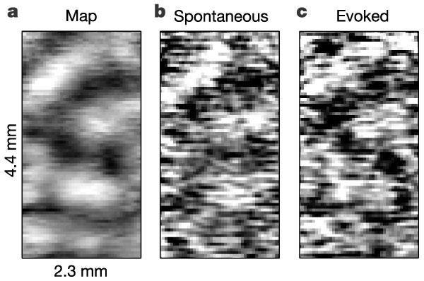
Figure 1: Reprinted by permission from Springer Nature: Nature. Spontaneously emerging cortical representations of visual attributes. Kenet et al. COPYRIGHT 2003. Activity corresponding closely to orientation maps spontaneously arises in the absence of input in an area with orientation selectivity. a) An orientation map of vertical orientation from cat area 18, where most cells are selective for stimulus orientation, obtained by using voltage sensitive dye imaging. b) A map obtained in a single frame from a spontaneous recording session. c) A single frame from an evoked session using the same orientation as for the map.

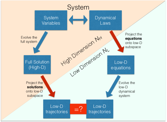
Figure 2: Schematics of Dimensionality Reduction

The general schematics of our dimensionality reduction approach is illustrated in (Fig. 2). At the top left we have the original system variables, which lives in dimension $N_{H}$, ruled by a high-dimensional dynamical law. At the bottom right, we have a low-dimensional space, the reduced variables, which live in dimension $N_{L}$. On the left branch, we first perform a detailed, costly and precise simulation of every variable in the system, and then we project this high-dimensional solution down into the lower-dimensional space. On the right branch, instead, we first project down the original high-dimensional vector field to obtain the reduced dynamics on the lower-dimensional subspace. We then evolve the reduced dynamics in its low-dimensional space. If both branches give rise to approximately the same low-D trajectories, then the reduction is well defined.

The structure of the paper is as follows. We first introduce some general definitions and the network structure of the specific example we will be using. We then review how the linear projection of the dynamics on the center space can be used for as a reduction approximation for certain simple cases Moirogiannis (2017), but also how it can fail for a wider range of parameters of the system. Next, we introduce the main focus of the paper, the proposed center manifold reduction technique, which can be thought as a nonlinear generalization of the linear projection on the center subspace. Finally, using the resulting approximations as numerical Ansatz to correct both the reduced dynamics equations in the case where the naive approximation fails as well as to describe the dynamics of individual units using the reduced dynamics.

II Definitions

Let us now establish the notation to be used in further detail, shown schematically in Fig. 3:

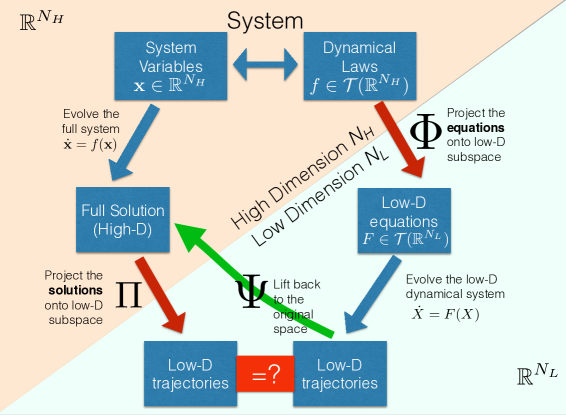
Figure 3: Operator Definitions

Again, at the top left we have our original full system: many variables $x\in{\mathbb{R}}^{N_{H}}$ ruled by a high-dimensional dynamical law $\dot{x}=f(x)$ given by a vector field $f$ in ${\mathbb{R}}^{N_{H}}$, stated as $f\in{\mathcal{T}}({\mathbb{R}}^{N_{H}})$. At the bottom right we have a low-dimensional space, the reduced variables, which live in ${\mathbb{R}}^{N_{L}}$. On the left branch we first evolve in $N_{H}$ and then we use a projection operator $\Pi$ to project the high-dimensional solution down into the lower-dimensional space On the right branch, instead, we first project down the high-dimensional vector field to obtain a reduced vector field $F$ on the lower-dimensional subspace: $F\in{\mathcal{T}}({\mathbb{R}}^{N_{L}})$. If we call the projector operator for the equations $\Phi$; then $F=\Phi\{f\}$. Then we evolve this simpler dynamics $\dot{X}=F(X)$. If both branches give rise to approximately the same low-D trajectories, then we can say we have reduced our system.

Moreover, we need a nontrivial reduction that retains enough information of the statistics of the system in the high-dimensional space. For instance, the diagram always commutes for a single point projection, which of course erases all information of the original system. Thus we define a lift operator $\Psi$ that describes the statistic of the original system as a function of the reduced dynamics.

We will demonstrate the above described methods using the following system of individual modules:

$$\dot{x} = w_{xx}x+w_{xy}y+f\left(x\right)$$ (1)

$$\dot{y} = w_{yx}x+w_{yy}y+g\left(y\right)$$

The nonlinearities are captured by the analytic functions $f$ and $g$ with $f\left(0\right)=g\left(0\right)=Df\left(0\right)=Dg\left(0\right)=0$.

Let $i\in\left\{1,2,\ldots,N\right\}$ be a parametrization of modules. We replicate the intramodule dynamics (1) for each of the $N$ modules and couple all modules through variable x with a linear connection matrix $M$ (and through layer y with a linear connection matrix $L$, but we will later consider $L=0$ ):

$$\dot{x}_{i} = w_{xx}x_{i}+w_{xy}y_{i}+f\left(x_{i}\right)+\underset{j}{\sum}M_{ij}x_{j}$$ (2)

$$\dot{y}_{i} = w_{yx}x_{i}+w_{yy}y_{i}+g\left(x_{i}\right)+\underset{j}{\sum}L_{ij}y_{j}$$

A common way to study such systems is to define $M_{ij}=\lambda G_{ij}$, where $\lambda$ is a global coupling constant and $G_{ij}$ a graph connectivity matrix, whose elements are either 0 or 1, which can be used to describe the connections as occurring only along an underlying lattice. This is a standard setting in physics, where the interaction strength is controlled by a physical constant and therefore affects all extant interactions in parallel. This approach leads to a changing effective dimensionality of the dynamical system, because as $\lambda$ is varied, all dynamical eigenvalues of the system move in unison, and hence the number of modes which can potentially enter the dynamics increases with increasing $\lambda$. We will take a different approach.

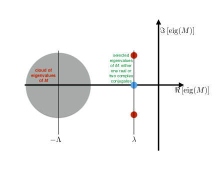
Figure 4: The Eigenvalues of $M$ in the Complex Plane The eigenvalues of $M$ in the complex plane. We shall construct $M$ so that most eigenvalues have strongly negative real parts, around $-d$, while either one real or two complex-conjugate eigenvalues with real part $\lambda$ will be allowed to approach the imaginary axis.

We shall assume the matrix $M_{ij}$ is under control from slow homeostatic processes, and we shall allow either one single real eigenvalue or a couple of complex-conjugate eigenvalues to increase and approach the stability limits from the left (Fig. 4). The classical approach of doing this in the field of random neural networks is by first generating a base matrix $M_{0}$ with a given controlled spectrum. Following a long history of modeling studies, one can assume $M_{0}$ to be given by suitably-scaled i.i.d. Gaussian random variables Sompolinsky (1998). Following this line of thought, in this work we shall either use $M_{0}$ as an $N\times N$ array of i.i.d Gaussians of variance $1/N$ (spectrum in the unit disk in the complex plane, matrix almost surely non-normal) or the antisymmetric component of said $M_{0}$, $M_{a}=(M_{0}-M^{t}_{0})/\sqrt{2}$ (purely imaginary spectrum, matrix is normal). The simplest way of then moving a single eigenvalue in the spectrum cloud independent of the rest of the eigenvalues and eigenvectors is the Brauer shift formula Brauer (1952):

$$M_{\mu}=M_{0}+(\lambda-\lambda_{0})({\textbf{vw}})$$ (3)

where $v$ and $w$ are the corresponding right and left eigenvectors.

We can use this formula to simulate this system with rest of the eigenvalues damping at any value or for simplicity we can assume that the rest of the eigensystem has strongly negative eigenvalues. For large enough $d\in\mathbb{R}^{+}$, $M=M_{0/a}-d{\textbf{I}}$ has the effect of moving the cloud of eigenvalues from a disk centered at zero to a disk centered at $-d$. We can then move a single real eigenvalue $\lambda\in\mathbb{R}$ (with $v$ and $w$ the corresponding right and left eigenvectors) to $\mu\in\mathbb{R}$ using the Brauer shift formula Brauer (1952):

$$M_{\mu}=M_{0/a}-d{\textbf{I}}+(d+\mu-\lambda)({\textbf{vw}})$$ (4)

or a pair of complex conjugate eigenvalues $\lambda,\>\bar{\lambda}$ to $\mu\pm im\left(\lambda\right)i$ :

$$M_{\mu}=M_{0/a}-d{\textbf{I}}+(d+\mu-Re\left(\lambda\right))({\textbf{vw}})+(d+\mu-Re\left(\bar{\lambda}\right))({\mathbf{\bar{v}\bar{w}}})$$ (5)

.

Antisymmetric matrices are normal. Thus consider $M$ to be given by eqn 4 with $M_{a}$, the antisymmetric component of a matrix of $N\times N$ i.i.d. Gausian variables of std $1/\sqrt{N}$; its eigenvalues are purely imaginary $\lambda=i\omega$ with imaginary component distributed like $p(\omega)\approx\sqrt{1-\omega^{2}/4}$. Consider one of its null eigenvalues (one is guaranteed to exist if $N$ is odd) and the corresponding eigenvector $v$. Then define as per Eq (4)

$$M_{\lambda}=M_{a}-dI+(d+\lambda)(\mathbf{vv^{\intercal}})$$ (6)

where the left (dual) eigenvector $\mathbf{w}$ of $\mathbf{v}$ is just it’s transpose $\mathbf{v}^{\intercal}$. All eigenvalues of $M$, except for the null one we chose, get moved to $-d$, while the null one now has value $\lambda$.

The Jacobian matrix at the fixed point $0$ is $J=\left[\begin{array}[]{c|c}M+w_{xx}I&w_{xy}I\\ \\ \hline\cr\\ w_{yx}I&L+w_{yy}I\end{array}\right]$.

Both intermodule and intramodule connectivity and their interplay is essential in evaluating the eigenvalues - eigenvectors pairs of the Jacobian. A useful tool for this evaluation is the following lemma:

Lemma 1: Let $W=\left[\begin{array}[]{c|c}M&w_{xy}I\\ \\ \hline\cr\\ w_{yx}I&L\end{array}\right]$ with $ML=LM$. Then :

(a) $Wv=\lambda v\iff\lambda^{2}-\left(\lambda_{M}+\lambda_{L}\right)\lambda+\left(\lambda_{M}\lambda_{L}-w_{xy}w_{yx}\right)=0\,\;\&\,\;v=\begin{pmatrix}u\\ \phi u\end{pmatrix},$ where $Mu=\lambda_{M}u,\,\;Nu=\lambda_{L}u$ and $\phi=\dfrac{\lambda-\lambda_{M}}{w_{xy}}=\dfrac{w_{yx}}{\lambda-\lambda_{L}}$ .

Proof: Trivial using that 2 matrices commute iff they are simultaneously diagonalizable. $\blacksquare$

The system as a whole, then, has a stability structure given by $2N$ eigenvalues that is a complex interplay of the structured column and the unstructured connections.

III Example Network Used in This Paper

We now consider a particular case which we can solve in pretty good detail, so as to concentrate on what are the central figures and concepts in this approach. Since each individual unit is 2-D obviously it cannot do much more than have a number of fixed points and limit cycles. In what follows we will deal exclusively with the following $N$ coupled identical damped oscillators $\left(\ddot{x}_{i}+F\left(x_{i}\right)\dot{x}_{i}+x_{i}=\underset{j}{\sum}M_{ij}\dot{x}_{j}\right)$, i.e. for $i\in\left\{1,\ldots N\right\}$:

$$\dot{x}_{i} = y_{i}+f\left(x_{i}\right)+\underset{j}{\sum}M_{ij}x_{j}$$ (7)

$$\dot{y}_{i} = -x_{i}$$

where $f\left(x\right)=$ $\underset{n\geq 2}{\sum}c_{n}x^{n}$ is analytic.

For example, in the special case $f(x)=-x^{3}$ we have $N$ coupled identical van der Pol oscillators:

$$\ddot{x}_{i}=-3\dot{x}_{i}x_{i}^{2}-x_{i}+\sum_{j}M_{ij}\dot{x}_{j}$$

We will show below we can evaluate the reduced dynamics for a Taylor series of $f$ order-by-order, so some of what follows concentrates on $f(x)=x^{\alpha}$. But the main issue is the structure of $M$, whether it’s normal or non-normal; and whether we control a single real or two complex-conjugate eigenvalues.

As we shall see shortly, our procedure for obtaining the global dynamics from the micro-scopic dynamics involves both the right and the left eigenvectors of $M$. In general the matrix of left eigenvectors is the inverse of the matrix of right eigenvectors. However if $M$ is normal, then the inverse reduces to the complex conjugate making their relationship much simpler. Therefore we shall explore first normal matrices and then examine the additional issues raised by non-normality. Within normal matrices we shall, as anticipated in (Fig. 4), either control a single real eigenvalue or two complex-conjugate ones.

We can evaluate the eigenvalue-eigenvector pairs of the Jacobian of the system from the corresponding eigenvalue-eigenvector pairs of $M$ using the following corollary:

Corollary 2: Let $W=\left[\begin{array}[]{c|c}M&w_{xy}I\\ \\ \hline\cr\\ w_{yx}I&0I\end{array}\right]$ with $w_{xy}w_{yx}<0$. Then:

(a) $Wv=\lambda v\iff\lambda+\dfrac{-w_{xy}w_{yx}}{\lambda}=\lambda_{M}\,\;\&\,\;v=\begin{pmatrix}\lambda u\\ w_{yx}u\end{pmatrix}$, where $Mu=\lambda_{M}u$

(b)$sign\left(Re\left(\lambda\right)\right)=sign\left(Re\left(\lambda_{M}\right)\right)$

(c)If $M$ has a zero eigenvalue , then $W$ has a pair of complex conjugate eigenvalues $\pm i\sqrt{-w_{xy}w_{yx}}$

(d)If M has a pair of complex conjugate eigenvalues $\pm\alpha i$ then $W$ has 2 pair of complex conjugate eigenvalues with 2 frequencies $\dfrac{\alpha\pm\sqrt{\alpha^{2}-4w_{xy}w_{yx}}}{2}$.

Proof: Trivia corollary of lemma 1 or see Hoppensteadt (2012) Theorem 12.1 for a similar statement. $\blacksquare$

IV Connectivity Matrix $M$

Let us assume that the elements of $M=\left(m_{i,j}\right)$ are independent randomly distributed gaussians of variance $\dfrac{1}{N}$ eg: $m_{i,j}\ i.i.d.\ \sim\mathcal{N}\left(0,\dfrac{1}{N}\right)$ with spectrum in the unit disk in the complex planeTao (2008). Let $\left\{V_{,1},\ldots,V_{,N}\right\}$ be the basis in $\mathbb{C}^{N\times 1}\cong C^{\mathrm{N}}$ of normalized right eigenvectors of $M\in\mathbb{R}^{N\times N}$ i.e. $MV=V\begin{pmatrix}\lambda_{1}&&0\\ &\ddots\\ 0&&\lambda_{N}\end{pmatrix}$ , where $V=\begin{bmatrix}V_{,1},&\cdots&,V_{,N}\end{bmatrix}\in\mathbb{C}^{N\times N}$. Let $\left\{W_{i,}=V_{,i}^{*}\right\}_{i\in\left\{1,\ldots N\right\}}$ be the dual basis of left eigenvectors of $M$ in $\mathbb{R}^{1\times N}\cong\left(\mathbb{R}^{\mathrm{N}}\right)^{*}$ (where $*:\mathbb{R^{\mathrm{N}}}\rightarrow\left(\mathbb{R}^{\mathrm{N}}\right)^{*}$ is the dual map induced by the bilinear form $<V_{,i},V_{,j}>=\delta_{i,j}$) i.e. $W=\begin{bmatrix}W_{1,}\\ \vdots\\ W_{N,}\end{bmatrix}=V^{-1}$.

For any $k\in\left\{1,\ldots,N\right\}$ and for any sequence of natural numbers of finite length $N$ : $p:\left\{1,\ldots,N\right\}\rightarrow\mathbb{N}$, and for a given ordered basis (in this case the right eigenvectors with a chosen ordering) let’s define:

$$\Gamma_{k}^{p}\coloneqq\underset{\varphi}{\sum}\left(V_{\varphi,k}\right)^{*}V_{\varphi,1}^{p\left(1\right)}\ldots V_{\varphi,N}^{p\left(N\right)}=\underset{\varphi}{\sum}W_{k,\varphi}V_{\varphi,1}^{p\left(1\right)}\ldots V_{\varphi,N}^{p\left(N\right)}=W_{k,}\times\underset{i}{\circledast}V_{,i}^{p\left(i\right)}$$ (8)

where $\times$ is matrix multiplication and $\circledast$ is element-wise multiplication (and the powers $V_{,i}^{p\left(i\right)}$ are elementwise).

In particular for the sequence $\delta_{i,\bullet}$ defined by $j\mapsto\delta_{i,j}$ (8) defines for $k=i$:

$$\Gamma_{i}^{k\delta_{i,\bullet}}\coloneqq\underset{\varphi}{\sum}\left(V_{\varphi,i}\right)^{*}V_{\varphi,i}^{k}=\underset{\varphi}{\sum}W_{i,\varphi}V_{\varphi,i}^{k}$$ (9)

As we will see these random variables play crucial role in describing the essential dynamics of the system. All the results in this part depend on $M$ only through the distribution of the $\Gamma_{k}^{p}$s and therefore can be extended to any connectivity type (for instance sparse matrices or only close neighbors connections) as long as we know the statistical properties of the $\Gamma_{k}^{p}$s. As we will see the limits:

$$\underset{N\rightarrow\infty}{\lim}\left(N^{\frac{n-1}{2}}\dfrac{n!}{k_{1}!\cdots k_{N}!}\Gamma_{\mu}^{\left(k_{1},\ldots,k_{N}\right)}\right)$$

where $n=k_{1}+\ldots+k_{N}$ are crucial, and in particular the limits: $\underset{N\rightarrow\infty}{\lim}\left(N^{\frac{k-1}{2}}\Gamma_{i}^{k\delta_{i,\bullet}}\right)$.

V Calculate $\Gamma$’s for Normal Matrix with Antisymmetric Gaussian i.i.d. Entries

In the case of normal matrices (9) can be written us:

$$\Gamma_{i}^{k\delta_{i,\bullet}}=\underset{\varphi}{\sum}V_{\varphi,i}^{k+1}$$ (10)

In the case of antisymmetric matrices we numerically observe that the elements of the eigenvectors approximate Gaussians of variance $\dfrac{1}{N}$ as $N\rightarrow\infty$ with:

$$\underset{N\rightarrow\infty}{\lim}\left(N^{\frac{k-1}{2}}\Gamma_{i}^{k\delta_{i,\bullet}}\right)=\begin{cases}\ k!!\ &k\text{ odd, }\\ \ 0&k\text{ even.}\end{cases}$$ (11)

given by the moments of Gaussian, where $k!!$ is the double factorial $k!!=1\cdot 3\cdots(k-2)\cdot k$. Similarly :

$$\underset{N\rightarrow\infty}{\lim}\left(N^{\frac{n-1}{2}}\dfrac{n!}{k_{1}!\cdots k_{N}!}\Gamma_{i}^{\left(k_{1},\ldots,k_{N}\right)}\right)=\dfrac{n!}{k_{1}!\cdots k_{N}!}\left(k_{1}-1\right)!!\cdots k_{i}!!\cdots\left(k_{N}-1\right)!!=n!!\begin{pmatrix}\frac{n-1}{2}\\ \frac{k_{1}}{2}\cdots\frac{k_{i}-1}{2}\cdots\frac{k_{N}}{2}\end{pmatrix}$$ (12)

if $k_{i}$ and $n$ are odd and $k_{j}$ for $j\neq i$ are even. Else $=0$. So the $\Gamma$’s are given by co-moments of independent Gaussians.

Let us notice that it is known that for random symmetric matrices (Gaussian orthogonal ensemble) eigenvectors are uniformly distributed in the sphere and independent of the eigenvalues (Corollary 2.5.4 in Anderson (2010)). This is implied by the invariance of the law of X under arbitrary orthogonal transformations as in our case. From O’Rourke (2016) we know that if $v$ is uniformly distributed on the sphere then $\lVert{v_{i}}\rVert^{2}\sim Beta\left(\dfrac{1}{2},\dfrac{N-1}{2}\right)$ and $\underset{N\rightarrow\infty}{\lim}\lVert{N^{\frac{p}{2}-1}\lVert{v}\rVert_{l_{p}}^{p}-E\lvert{N\left(0,1\right)}\rvert}^{p}\rVert=0$ almost surely.

VI Linear Projection onto the Stable and the Center Spaces - Definitions

Let $X_{\lambda_{k}}=\dfrac{1}{\sqrt{N}}W_{k,}\times\begin{pmatrix}x_{1}\\ \vdots\\ x_{n}\end{pmatrix}=\dfrac{1}{\sqrt{N}}\underset{i}{\sum}W_{k,i}x_{i}$ be the normalized (so that $X_{\lambda_{k}}$ is of order 1, because ${x\cdot x}\approx N$ while if $M$ is normal $\ W_{k,}\cdot W_{k,}=1$ so that ${W_{k,}\cdot x}\approx\sqrt{N}$ generically.) coordinates of activity in the basis of right eigenvalues, so :

$$x=\begin{pmatrix}x_{1}\\ \vdots\\ x_{N}\end{pmatrix}=\sqrt{N}V\begin{pmatrix}X_{\lambda_{1}}\\ \vdots\\ X_{\lambda_{N}}\end{pmatrix}=\sqrt{N}\underset{i}{\sum}X_{\lambda_{i}}V_{,i}$$ (13)

where $V_{,i}$, for $i=1,...,N$ are the right eigenvectors, columns of the matrix $V$.

Applying $\dfrac{1}{\sqrt{N}}W$ to equations (7) we have, for an eigenvalue $\mu\in spec\left(M\right)$ :

$$\dot{X}_{\mu} = \dfrac{1}{\sqrt{N}}\underset{i}{\sum}W_{\mu,i}f\left(x_{i}\right)+Y_{\mu}+\mu X$$ (14)

$$\dot{Y}_{\mu} = -X_{\mu}$$

Equation (14) will be essential in defining the operator $\Phi$ as seen in (Fig. 3). Equation (13) will be essential in defining the operator $\Psi$.

The Hartman–Grobman theorem only holds for hyperbolic equilibriums, so as eigenvalues move close to the critical boundary, the nonlinearities:

$$F_{\mu}\coloneqq\dfrac{1}{\sqrt{N}}\underset{i}{\sum}W_{\mu,i}f\left(x_{i}\right)=\dfrac{1}{\sqrt{N}}\underset{i}{\sum}W_{\mu,i}f\left(\sqrt{N}\underset{k}{\sum}V_{i,k}X_{\lambda_{k}}\right)$$ (15)

became essential in describing the dynamics.

Equations (7) (similarly for the general equations (2)) can be written in the basis of right eigenvectors corresponding to the eigenvalues, for $\mu\in spec\left(M\right)$:

$$\dot{X}_{\mu}=F_{\mu}\left(X_{\lambda_{1}},\ldots,X_{\lambda_{N}}\right)+Y_{\mu}+\mu X_{\mu}$$ (16)

$$\dot{Y}_{\mu}=-X_{\mu}$$

where

$$F_{\mu_{i}}\left(X_{\lambda_{1}},\ldots,X_{\lambda_{N}}\right)=\underset{n\geq 2}{\sum}c_{n}\sum_{k_{1}+\ldots+k_{N}=n}\left(\dfrac{n!}{k_{1}!\cdots k_{N}!}{\sqrt{N}}^{\left(n-1\right)}\Gamma_{\mu}^{\left(k_{1},\ldots,k_{N}\right)}\right)X_{\lambda_{1}}^{k_{1}}\cdots X_{\lambda_{N}}^{k_{N}}$$ (17)

VII Naive Approach - Single Real Eigenvalue, Normal Matrix

Let us consider the system (7) as a single real eigenvalue of M, $\lambda=\lambda_{1}\in\mathbb{R}$, crosses the imaginary axis (4) (the critical boundary for this case, look at corollary 2) becoming slightly positive, while the rest of the eigenvalues $\mu\in\left\{\lambda_{2},\ldots,\lambda_{N}\right\}$ have negative real part. The naive approximation would be to consider $X_{\mu}\approx 0$ for $\mu\in spec\left(M\right)\setminus\left\{\lambda\right\}$ and we can reduce the $2N$-dimensional system (7) into the 2-dimensional system :

$$\dot{X} = F(x)+Y+\mu X$$ (18)

$$\dot{Y} = -X$$

Where $X\coloneqq X_{\lambda}$ , $Y\coloneqq Y_{\lambda}$ and $F(x)$ is given by (15):

$$F(x)\coloneqq F_{\lambda}(x)=\dfrac{1}{\sqrt{N}}\underset{i}{\sum}W_{\lambda,i}f\left(x_{i}\right)=\dfrac{1}{\sqrt{N}}\underset{i}{\sum}W_{\lambda,i}f\left(\sqrt{N}V_{i,1}X+\sqrt{N}\underset{\mu\in spec\left(M\right)\setminus\left\{\lambda\right\}}{\sum}V_{i,\mu}X_{\mu}\right)$$ (19)

Evaluation of the $\underset{i}{\sum}W_{\lambda,i}f\left(x_{i}\right)$ term is the key; assuming conversely that the projection of $x_{i}$ onto the complement of $V_{,1}$ (space perpendicular to $V_{,1}$ in the normal case) is small (an assumption we shall revisit in detail below) we’d get an ansatz which is our first, naive approximation of the lift operator $\Psi$, which gives the coordinates in the full space as a function of the coordinates on the center manifold ${x}=\Psi[X]$:

$$x_{i} \approx \sqrt{N}XV_{i,1}$$ (20)

$$y_{i} \approx \sqrt{N}YV_{i,1}$$

Then (18) can be written us :

$$\dot{X} = F(X)+Y+\mu X$$ (21)

$$\dot{Y} = -X$$

Where :

$$F(X)=\dfrac{1}{\sqrt{N}}\underset{i}{\sum}W_{\lambda,i}f\left(\sqrt{N}V_{i,1}X\right)$$ (22)

The coarse-graining operator $\Phi$, which transforms the original full dimensional dynamics to the coarsened, low-dimensional dynamics is defined by

$$F\equiv\Phi[f]$$

In other words the $2N$ dimensional equation (14) is reduced to the 2 dimensional equation:

$$\dot{X}_{\lambda} = \underset{k\geq 2}{\sum}\left(c_{k}{\sqrt{N}}^{\left(k-1\right)}\Gamma_{\lambda}^{k\delta_{1,\bullet}}\right)X_{\lambda}^{k}+Y_{\lambda}+\lambda X_{\lambda}$$ (23)

$$\dot{Y}_{\lambda} = -X_{\lambda}$$

We see that the dynamics of $X_{\lambda}$ is determined by the random variables: $\sqrt{N}^{(k-1)}\Gamma_{\lambda}^{k\delta_{1,\bullet}}=\sqrt{N}^{(k-1)}\underset{\varphi=1}{\overset{N}{\sum}}W_{1,\varphi}V_{\varphi,1}^{k}$ where $V_{\cdotp,1}$ is normalized so that $\underset{\varphi}{\sum}V_{\varphi,1}^{2}=1$ :

In the case of normal matrices and $f\left(x\right)=$ $\underset{n\geq 2}{\sum}c_{n}x^{n}$ analytic we have:

$$F\left(X\right)=\dfrac{1}{\sqrt{N}}\underset{\varphi=1}{\overset{N}{\sum}}W_{1,\varphi}f\left(V_{\varphi,1}\sqrt{N}X\right)=\underset{k\geq 1}{\sum}\left(c_{2k+1}\left(2k+1\right)!!\right)X^{2k+1}$$ (24)

.

The first thing to notice is that $\Phi$ is linear in $f$, meaning we can try to apply it order-by-order in a Taylor expansion of $f$. Applying Eq (22) to individual integer powers yields, in the large $N$ limit, an evaluation of the moments of a Gaussian distribution:

$$\Phi[x^{\alpha}]=X^{\alpha}N^{{\alpha-1}\over 2}\sum_{i}e_{i}^{\alpha+1}=\begin{cases}\ \alpha!!\ X^{\alpha}&\alpha\text{ odd, }\\ \qquad 0&\alpha\text{ even.}\end{cases}$$ (25)

The most important property to note is that the result is independent of which eigenvector $v$ we chose, because under these circumstances the operator is self-averaging. Then, the power-law is unchanged except for a prefactor: the cubic $X^{3}$ nonlinearity gets renormalized by a factor of 3, $X^{5}$ by 15, $X^{7}$ by 105. Curiously this operator destroys all even nonlinearities. As we shall see later the even nonlinearities get absorbed in the overall shape of the center manifold, which we have assumed in the ansatz Eq (20) to be linear in $x_{i}$. However the naive reduced equations Eq (18) are not affected.

We first simulate randomly coupled Van der Pol oscillators given by Eq (7) with $f(x)=-x^{3}$ and for random matrix $M$ defined using Eq (6) with $N=351$ and $d=-30$. We let $\lambda=0.1$ cross the real line by a small value. We numerically integrate the whole system for random initial values and let it settle after a transient on the limit cycle. In movie: https://drive.google.com/open?id=14ku9fZlCUAW_mzEHIvezkRw4G6fbAAix we plot at each time frame $t$ the values $\{(x_{i}(t),y_{i}(t))\arrowvert i\in\{1,\ldots,N\}$ as black dots. Moreover for each $i$ we plot as a thin black line the orbit of $(x_{i},y_{i})$ for a short time past interval $(t-\Delta t,t)$ to visualize the orbits. We plot with a green cycle $(X_{\lambda},Y_{\lambda})$ the linear projection of $x$ and $y$ in the critical eigenvector and with a red cross the simulation of Eq (21) with $F(X)=-3X^{3}$ (and initial condition the linear projections on the critical mode of the initial conditions used for the high dimensional Eq (7)). Snapshots of the simulation movie are shown in (Fig 5). As in the case of individual orbits we also plot part of the past orbits for visualization with green and red colors respectable. As we can see in this case diagram (Fig. 3) using our naive definition of our $\Phi$ operator Eq (25). Moreover we see that the cubic nonlinearity doesn’t survive in the lift $\Psi$ a statement that we shall see theoretically shortly.

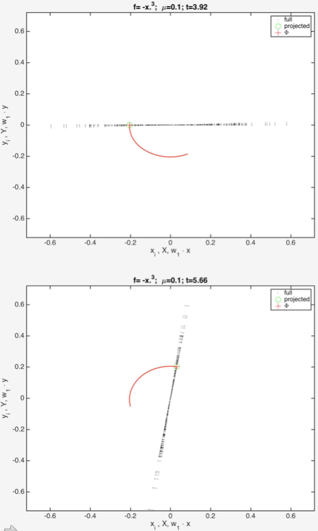
Figure 5: Naive $\Phi$ - Linear $\Psi$ Randomly coupled Van der Pol oscillators given by Eq (7) with $f(x)=-x^{3}$ and for random matrix $M$ defined using Eq (6) with $N=351$ and $d=-30$. We let $\lambda=0.1$ cross the real line by a small value.

In movie: https://drive.google.com/open?id=1Ldn_YvlXaCSRc9L3dS_5smrh_39OqzOP we can see the corresponding simulation for $f(x)=x^{2}-x^{3}$. Snapshots of the simulation movie are shown in (Fig. 6). As we can see the added even nonlinearity doesn’t survive in the $\Phi$ operator and our approximation is still accurate (as we will see later a more accurate statement would be that the even nonlinearity doesn’t survive as an even nonlinearity but can have small "leak" into higher order odd nonlinearities). But in this case it becomes apparent that the naive linear approximation of $\Psi$ Eq (20) fails and the even nonlinearity survives in the operator. We will see that theoretically shortly.

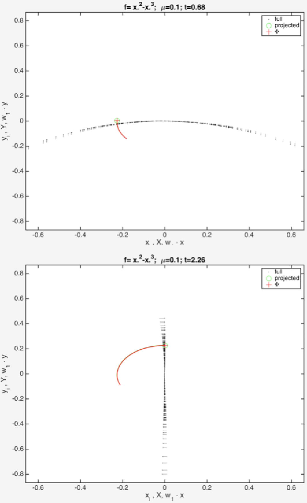
Figure 6: Naive $\Phi$ - Nonlinear $\Psi$ Randomly coupled Van der Pol oscillators given by Eq (7) with $f(x)=x^{2}-x^{3}$ and for random matrix $M$ defined using Eq (6) with $N=351$ and $\Lambda=-30$. We let $\lambda=0.1$ cross the real line by a small value.

VIII Failure of Above

The above approximation is studied in Moirogiannis (2017) and assumes that the center space $E^{c}=\mathbb{R}\begin{pmatrix}v_{1}\\ 0\end{pmatrix}\oplus\mathbb{R}\begin{pmatrix}0\\ v_{1}\end{pmatrix}$ is invariant which is only true up to linear approximation. In fact the nonlinearities of the invariant center manifolds tangent to $E_{c}$ can change the qualitative behavior of the reduced to the manifold dynamics and there are examples that show that the above naive linear projection fails to capture the reduced dynamics Guckenheimer (2013). In our model particularly equations (23) predict that the Hopf bifurcation is supercritical iff $c_{3}<0$ independently of the value of $c_{2}$ but as numeric simulations show and as we will prove later the bifurcation is supercritical for large enough $\left|c_{2}\right|$.

We can see the failure of our naive $\Phi$ approximation Eq (25) by simulating a system as in the last movie with a higher order of even nonlinearity $f(x)=4.1*x^{2}-x^{3}$. We can see this in movie: https://drive.google.com/open?id=1FpkxPm5kRCjHi_TSl_5Mrk3Jn6HQgAlr. Snapshots of the simulation movie are shown in (Fig. 7).

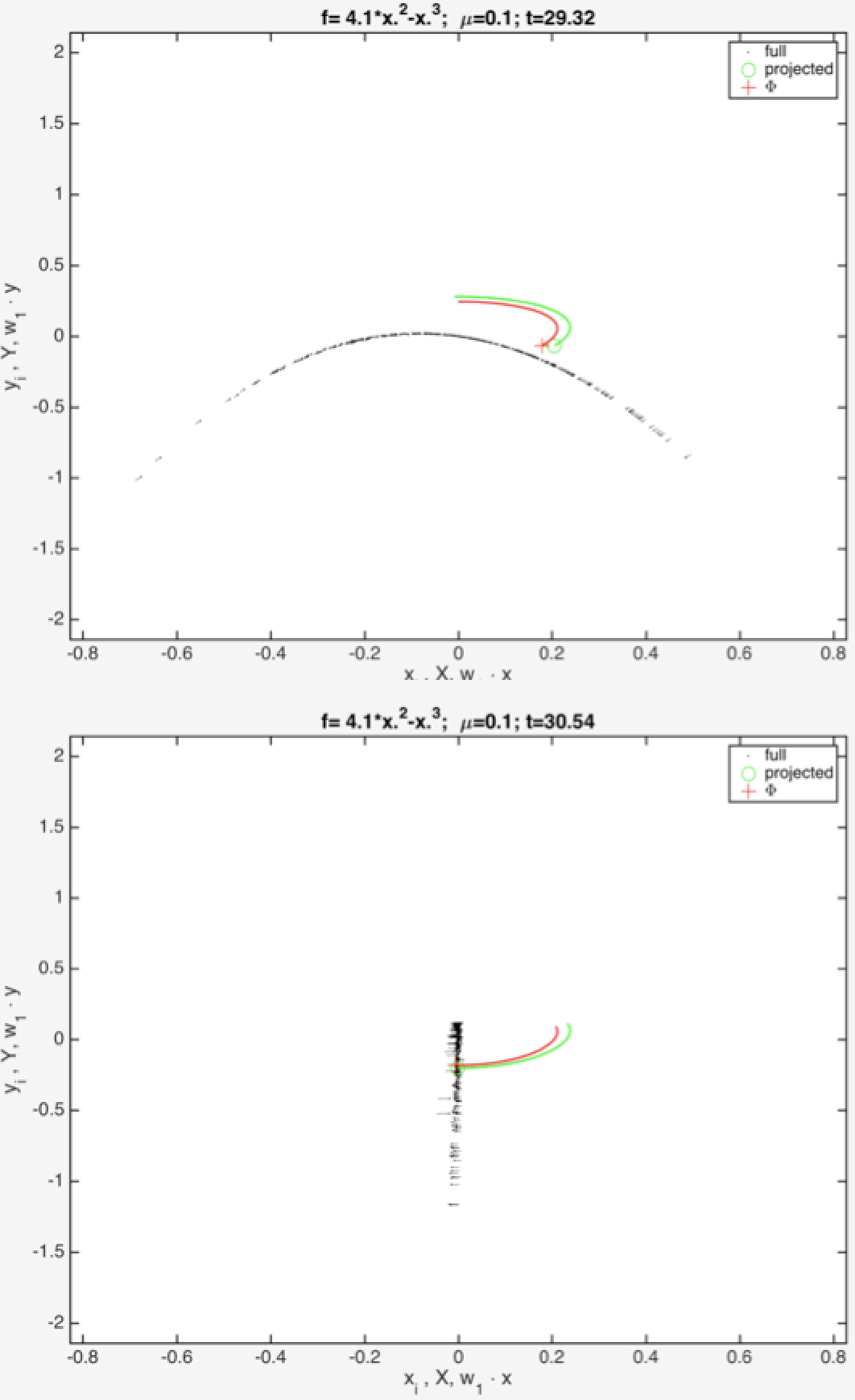
Figure 7: Naive $\Phi$ Fail Randomly coupled Van der Pol oscillators given by Eq (7) with $f(x)=4.1*x^{2}-x^{3}$ and for random matrix $M$ defined using Eq (6) with $N=351$ and $\Lambda=-30$. We let $\lambda=0.1$ cross the real line by a small value.

IX Center Manifold Reduction

We will follow similar notation and approach as in Hoppensteadt (2012) , in particular look at section 12.7 for the 3rd order approximation of $\psi$ for $f\left(x\right)=x^{2}$ and 2nd order approximation of $\psi$ for $f\left(x\right)=\pm x^{3}$ in the case of symmetric interaction matrix. Here we care about more general forms of matrices and for any abstract nonlinearity. For more details on center manifolds look at Ioos (1999) or for formal proofs at Carr (2012).

We can rewrite equation (7) as:

$\eqref{eq:leyerx}\Leftrightarrow\quad$ : $\dot{Z}=G\left(Z\right)=WZ+F\left(Z\right)$

where $Z=\left(\begin{array}[]{c}x_{1}\\ \vdots\\ x_{N}\\ y_{1}\\ \vdots\\ y_{N}\end{array}\right)\in\mathbb{R}^{2N},\quad W=\left(\begin{array}[]{c|c}M&I\\ \\ \hline\cr\\ -I&0\end{array}\right),\quad F\left(Z\right)=\left(\begin{array}[]{c}f\left(x_{1}\right)\\ \vdots\\ f\left(x_{N}\right)\\ 0\\ \vdots\\ 0\end{array}\right)$ .

Let us assume that a single real eigenvalue of M, $\lambda=\lambda_{1}\in\mathbb{R}$ (with corresponding right eigenvector $v_{1}$) crosses the imaginary axis. Corollary 2 implies that the corresponding eigenvalues of the whole system are $\pm i$ with corresponding eigenvectors $\begin{pmatrix}\pm iv_{1}\\ -v_{1}\end{pmatrix}$. Let $E^{c}=\mathbb{R}\begin{pmatrix}v_{1}\\ 0\end{pmatrix}\oplus\mathbb{R}\begin{pmatrix}0\\ v_{1}\end{pmatrix}=\left\{x\begin{pmatrix}v_{1}\\ 0\end{pmatrix}+y\begin{pmatrix}0\\ v_{1}\end{pmatrix}\mid x,y\in\mathbb{R}\right\}$ be the center space, $E^{s}=E^{\lambda_{2}}\oplus\ldots\oplus E^{\lambda_{N}}=$$\mathbb{R}\left(\begin{array}[]{c}\upsilon_{2}\\ 0\end{array}\right)\oplus\mathbb{R}\begin{pmatrix}0\\ v_{2}\end{pmatrix}\oplus\ldots\oplus\mathbb{R}\left(\begin{array}[]{c}\upsilon_{N}\\ 0\end{array}\right)\oplus\mathbb{R}\begin{pmatrix}0\\ v_{N}\end{pmatrix}$ be the stable space, $\Pi_{c}=\begin{pmatrix}v_{1}w_{1}&0\\ 0&v_{1}w_{1}\end{pmatrix}:\mathbb{R}^{2N}=E^{c}\oplus E^{s}\rightarrow E^{c}$ , $\Pi_{\lambda_{k}}=\begin{pmatrix}v_{k}w_{k}&0\\ 0&v_{k}w_{k}\end{pmatrix}:\mathbb{R}^{2N}\rightarrow E^{\lambda_{k}}$ and $\Pi_{s}=\Pi_{\lambda_{2}}+\ldots+\Pi_{\lambda_{k}}:\mathbb{R}^{2N}=E^{c}\oplus E^{s}\rightarrow E^{s}$ the defined by the basis projections. The above projections commute with $W$ since they have the same eigenspaces.

The center manifold theorem ensures that there is a local mapping $\psi:E^{c}\rightarrow E^{s}$ with

$$\psi(0)=0\quad and\quad D\psi(0)=0$$

such that the manifold $\mathcal{M}$ defined by:

$$\mathcal{M}=\left\{u+\psi\left(u\right)\mid u\in E_{c}\right\}=\left\{x\begin{pmatrix}v_{1}\\ 0\end{pmatrix}+y\begin{pmatrix}0\\ v_{1}\end{pmatrix}+\psi\left(x,y\right)\mid x,y\in\mathbb{R}\right\}$$

is invariant and locally attractive (emergence theorem). The dynamics reduced on $\mathcal{M}$ are locally:

$$\dot{u}=\Pi_{c}G\left(u+\psi\left(u\right)\right)=Wu+\Pi_{c}F\left(u+\psi\left(u\right)\right)$$ (26)

A schematic of a center manifold and the invariance equations can be seen in (Fig. 8). Using the approximation theorem, we can approximate $\psi$ to any order from the equation:

$$D\psi(u)\left(Wu+\Pi_{c}F\left(u+\psi\left(u\right)\right)\right)=D\psi(u)\dot{u}=\Pi_{s}G\left(u+\psi\left(u\right)\right)=W\psi\left(u\right)+\Pi_{s}F\left(u+\psi\left(u\right)\right)$$ (27)

More precisely, if $Dh(u)\left(Wu+\Pi_{c}F\left(u+h\left(u\right)\right)\right)-Wh\left(u\right)+\Pi_{s}F\left(u+h\left(u\right)\right)=O\left(\left|u\right|^{k}\right)$ then $\psi\left(u\right)=h\left(u\right)+O\left(\left|u\right|^{k}\right)$.

$\psi$ approximated by (27) is used to define the lift operator $\Psi_{f}$ and equation (26) defines the reduction operator $\Phi$.

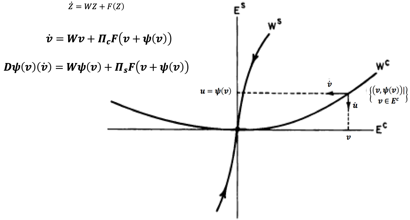
Figure 8: Center Manifold Reduction A schematic of center manifold and the invariance equations.

This gives us an algorithm of calculating orders of increasingly degree in the Taylor expansions of both reduced dynamics and the center manifold embedding by iteratively interchanging equations (26) : $\dot{u}=Wu+\Pi_{c}F\left(u+\psi\left(u\right)\right)$ and (27) : $D\psi(u)\dot{u}=W\psi\left(u\right)+\Pi_{s}F\left(u+\psi\left(u\right)\right)$ correspondingly. However this algorithm can be complicated. As the dimension of the center manifold increases (or order of desired approximation increases) the calculations become intractable (the number of unknown parameters and resulting equations grows like $\begin{pmatrix}dimension+order-1\\ order\end{pmatrix},$ the number of parameters to keep track of $\sim$$\underset{r<order}{\sum}\begin{pmatrix}dimension+r-1\\ r\end{pmatrix}$ + all combinations with repetitions of those up to the specified $order$). So using symbolic algorithms is essential Freire (1988) .

X $n$ th Order Approximation of $\Psi$ for $f\left(x\right)=c_{n}x^{n}+O\left(x^{n+1}\right)$

Even though those questions are in general complicated, when estimating the first nonlinear order of approximation for the center manifold embedding and reduced dynamics on it of (7) with $f\left(x\right)=c_{n}x^{n}+O\left(x^{n+1}\right)$ the corresponding equations are very simple.

Let $\psi\left(\begin{pmatrix}v_{1}\\ 0\end{pmatrix}x+\begin{pmatrix}0\\ v_{1}\end{pmatrix}y\right)=\underset{k=2}{\overset{N}{\sum}}\left(\begin{array}[]{c}\left(\underset{i=0}{\overset{n}{\sum}}\alpha_{i}^{k}x^{n-i}y^{i}\right)V_{,k}\\ \left(\underset{i=0}{\overset{n}{\sum}}\beta_{i}^{k}x^{n-i}y^{i}\right)V_{,k}\end{array}\right)+O\left(\left(\sqrt{x^{2}+y^{2}}\right)^{n}\right)$ , and for convenience let $\alpha_{-1}=\alpha_{n+1}=\beta_{-1}=\beta_{n+1}=0$.

Then $D\psi\left(u\right)\dot{u}=\underset{k=2}{\overset{N}{\sum}}\left(\begin{array}[]{c}\left(\underset{i=0}{\overset{n}{\sum}}\left(\left(n-i+1\right)\alpha_{i-1}^{k}-\left(i+1\right)\alpha_{i+1}^{k}\right)x^{n-i}y^{i}\right)V_{,k}\\ \left(\underset{i=0}{\overset{n}{\sum}}\left(\left(n-i+1\right)\beta_{i-1}^{k}-\left(i+1\right)\beta_{i+1}^{k}\right)x^{n-i}y^{i}\right)V_{,k}\end{array}\right)+O\left(\left(\sqrt{x^{2}+y^{2}}\right)^{n}\right)$ ,

$W\psi\left(u\right)=\underset{k=2}{\overset{N}{\sum}}\left(\begin{array}[]{c}\left(\underset{i=0}{\overset{n}{\sum}}\left(\lambda_{k}\alpha_{i}^{k}+\beta_{i}^{k}\right)x^{n-i}y^{i}\right)V_{,k}\\ \left(\underset{i=0}{\overset{n}{\sum}}-\alpha_{i}^{k}x^{n-i}y^{i}\right)V_{,k}\end{array}\right)+O\left(\left(\sqrt{x^{2}+y^{2}}\right)^{n}\right)$ ,

$\Pi_{s}F\left(u+\Psi\left(u\right)\right)=c_{n}\Pi_{s}\left(\begin{array}[]{c}\left(V_{1,1}x+O\left(n+1\right)\right)^{n}\\ \vdots\\ \left(V_{N,1}x+O\left(n+1\right)\right)^{n}\\ 0\\ \vdots\\ 0\end{array}\right)=c_{n}\Pi_{s}\left(\begin{array}[]{c}\left(V_{1,1}x\right)^{n}\\ \vdots\\ \left(V_{N,1}x\right)^{n}\\ 0\\ \vdots\\ 0\end{array}\right)+O\left(n+1\right)=c_{n}x^{n}\underset{k=2}{\overset{N}{\sum}}V_{,k}\varGamma_{k}^{n\delta_{1,\bullet}}+O\left(n+1\right)$.

Projecting equation (27) onto the stable modes using $\Pi_{\lambda_{k}}$ for $k\geq 2$ gives us the equations:

$$\begin{pmatrix}\alpha_{0}^{k}\\ \vdots\\ \alpha_{n}^{k}\end{pmatrix} = A\begin{pmatrix}\beta_{0}^{k}\\ \vdots\\ \beta_{n}^{k}\end{pmatrix}$$ (28)

$$\left(-\lambda_{k}id_{n}-A\right)\begin{pmatrix}\alpha_{0}^{k}\\ \vdots\\ \alpha_{n}^{k}\end{pmatrix}-\begin{pmatrix}\beta_{0}^{k}\\ \vdots\\ \beta_{n}^{k}\end{pmatrix} = \begin{pmatrix}c_{n}\varGamma_{k}^{n\delta_{1,\bullet}}\\ \vdots\\ 0\end{pmatrix}$$

where $A=\begin{pmatrix}0&1\\ -n&0&2\\ &-(n-1)&0&\ddots\\ &&\ddots&\ddots&\ddots\\ &&&\ddots&0&n-1\\ &&&&-2&0&n\\ &&&&&-1&0\end{pmatrix}$ .

If $f\left(x\right)=c_{2}x^{2}+O\left(x^{3}\right)$ then after scaling normalization we get:

$$\Psi\left(\begin{pmatrix}v_{1}\\ 0\end{pmatrix}x+\begin{pmatrix}0\\ v_{1}\end{pmatrix}y\right)=$$ (29)

$$=\underset{k=2}{\overset{N}{\sum}}c_{2}{\sqrt{N}}\varGamma_{k}^{2\delta_{1,\bullet}}\begin{pmatrix}\left(\dfrac{-2\lambda_{k}}{4\lambda_{k}^{2}+9}x^{2}+\dfrac{-6}{4\lambda_{k}^{2}+9}xy+\dfrac{2\lambda_{k}}{4\lambda_{k}^{2}+9}y^{2}+O\left(3\right)\right)V_{,k}\\ \left(\dfrac{-\left(2\lambda_{k}^{2}+3\right)}{4\lambda_{k}^{2}+9}x^{2}+\dfrac{-2\lambda_{k}}{4\lambda_{k}^{2}+9}xy+\dfrac{-\left(2\lambda_{k}^{2}+6\right)}{4\lambda_{k}^{2}+9}y^{2}+O\left(3\right)\right)V_{,k}\end{pmatrix}$$ (30)

If $f(x)=c_{3}x^{3}+O\left(x^{4}\right)$ then after scaling normalization we get:

$$\Psi\left(\begin{pmatrix}v_{1}\\ 0\end{pmatrix}x+\begin{pmatrix}0\\ v_{1}\end{pmatrix}y\right)=$$ (31)

$$=\underset{k=2}{\overset{N}{\sum}}c_{3}{\sqrt{N}}^{2}\varGamma_{k}^{3\delta_{1,\bullet}}\begin{pmatrix}\left(\dfrac{-9\lambda_{k}^{2}-48}{9\lambda_{k}^{3}+64\lambda_{k}}x^{3}-\dfrac{18\lambda_{k}}{9\lambda_{k}^{3}+64\lambda_{k}}x^{2}y+\dfrac{-48}{9\lambda_{k}^{3}+64\lambda_{k}}xy^{2}-\dfrac{-6\lambda_{k}}{9\lambda_{k}^{3}+64\lambda_{k}}y^{3}+O\left(4\right)\right)V_{,k}\\ \left(\dfrac{2\lambda_{k}}{9\lambda_{k}^{3}+64\lambda_{k}}x^{3}+\dfrac{-9\lambda_{k}^{2}-48}{9\lambda_{k}^{3}+64\lambda_{k}}x^{2}y+\dfrac{-6\lambda_{k}}{9\lambda_{k}^{3}+64\lambda_{k}}xy^{2}+\dfrac{-6\lambda_{k}^{2}-48}{9\lambda_{k}^{3}+64\lambda_{k}}y^{3}+O\left(4\right)\right)V_{,k}\end{pmatrix}$$ (32)

Let us notice that for the matrix $M$ generated as in (6) we have that for $\Lambda\rightarrow\infty$ the 3rd order nonlinearity (odd) doesn’t survive on the shape of the center manifold while the 2nd order nonlinearity (even) survives only on the second "layer" and only as even in both $x$ and $y$. This is not a general result but comes from the interplay between the vertical (module) and horizontal (M) connectivity. For instance similar calculations for coupled simple, unstructured $1D$ subunits gives a center manifold where even the even nonlinearities go to 0 when $\Lambda\rightarrow\infty$.

XI Symmetries of $\alpha$’s and $\beta$’s

The above observation for the first order of approximation of $Psi$ is more general. In particular we can show that: $\alpha_{i}^{k}=\dfrac{P_{a,k,i}}{P}$, and $\beta_{i}^{k}=\dfrac{P_{\beta,k,i}}{P},$ where $P$ is a polynomial of $\lambda_{k}$ of order $k$ and $P_{\alpha,k,i}$ , $P_{\beta,k,i}$ polynomials of order $\leq k$. The inequality is streak except for $P_{\beta,k,i}$ when $k$ and $i$ are even. That would imply that for large $\Lambda$ only even nonlinearities survive by the operate $\Psi$ as even nonlinearities on the $y$ layer (the layer in which the original equations don’t include nonlinearities). We will talk about this in details elsewhere but let us just notice that the coefficients are just determined by determinants of submatrices of the pentadiagonal $A^{2}+\lambda_{k}A+id_{n}$ where:

  $A^{2}=$

$$\left(\begin{array}[]{ccccccccccccc}-n&0&1\cdot 2&0\\ 0&-n\cdot 1-2\cdot\left(n-1\right)&0&2\cdot 3\\ n\cdot\left(n-1\right)&0&-\left(n-1\right)\cdot 2-3\cdot\left(n-2\right)&0&\ddots\\ 0&\left(n-1\right)\cdot\left(n-2\right)&0&\ddots\\ &&\ddots&&\ddots&&\left(k-1\right)\cdot k\\ &&&&&\ddots&0&k\cdot\left(k+1\right)\\ &&&&\left(n+2-k\right)\cdot\left(n+1-k\right)&0&-\left(n+1-k\right)\cdot k-\left(k+1\right)\cdot\left(n-k\right)&0&\left(k+1\right)\cdot\left(k+2\right)\\ &&&&&\left(n+1-k\right)\cdot\left(n-k\right)&0\\ &&&&&&\left(n-k\right)\cdot\left(n-k-1\right)&&&&\ddots\\ &&&&&&&&&\ddots&0&\left(n-2\right)\cdot\left(n-1\right)&0\\ &&&&&&&&\ddots&0&-3\cdot\left(n-2\right)-\left(n-1\right)\cdot 2&0&\left(n-1\right)\cdot n\\ &&&&&&&&&3\cdot 2&0&-2\cdot\left(n-1\right)-n\cdot 1&0\\ &&&&&&&&0&2\cdot 1&0&-n\end{array}\right)1$$ (46)

XII Reduced Dynamics 3rd Order Approximation

Let $f\left(x\right)=c_{2}x^{2}+c_{3}x^{3}+O\left(x^{4}\right)$ , then:

The reduced equations (26) are then up to order 3:

$$\begin{pmatrix}v_{1}\\ 0\end{pmatrix}\dot{x}+\begin{pmatrix}0\\ v_{1}\end{pmatrix}\dot{y}=W\begin{pmatrix}v_{1}\\ 0\end{pmatrix}x+W\begin{pmatrix}0\\ v_{1}\end{pmatrix}y+$$

$$+c_{2}\Pi_{c}\left(\begin{pmatrix}\left(V_{1,1}x+\underset{k=2}{\overset{N}{\sum}}V_{1,k}\left(\alpha_{0}^{k}x^{2}+\alpha_{1}^{k}xy+\alpha_{2}^{k}y^{2}\right)\right)^{2}\\ \vdots\\ \left(V_{N,1}x+\underset{k=2}{\overset{N}{\sum}}V_{N,k}\left(\beta_{0}^{k}x^{2}+\beta_{1}^{k}xy+\beta_{2}^{k}y^{2}\right)\right)^{2}\\ 0\\ \vdots\\ 0\end{pmatrix}\right)+c_{3}\Pi_{c}\left(\begin{pmatrix}\left(V_{1,1}x\right)^{3}\\ \vdots\\ \left(V_{N,1}x\right)^{3}\\ 0\\ \vdots\\ 0\end{pmatrix}\right)+O\left(4\right)$$

So after scaling normalization we get the reduced dynamics equations:

$$\dot{x} = y+c_{2}{\sqrt{N}}\Gamma_{1}^{2\delta_{1,\bullet}}x^{2}+\left(c_{3}{\sqrt{N}}^{2}\varGamma_{1}^{3\delta_{1,\bullet}}+2c_{2}{\sqrt{N}}^{2}\underset{k=2}{\overset{N}{\sum}}\Gamma_{1}^{\delta_{1,\bullet}+\delta_{k,\bullet}}\alpha_{0}^{k}\right)x^{3}+$$

$$+\left(2c_{2}{\sqrt{N}}^{2)}\underset{k=2}{\overset{N}{\sum}}\Gamma_{1}^{\delta_{1,\bullet}+\delta_{k,\bullet}}\alpha_{1}^{k}\right)x^{2}y++\left(2c_{2}{\sqrt{N}}^{2}\underset{k=2}{\overset{N}{\sum}}\Gamma_{1}^{\delta_{1,\bullet}+\delta_{k,\bullet}}\alpha_{2}^{k}\right)xy^{2}+O\left(4\right)$$

$$\dot{y} = -x$$

Proposition 3: Let $M_{0}$ with $\lambda_{1}=0,$ $Re\left(\lambda_{i}\right)<0$ for $i>1$ and $M\left(\mu\right)=M_{0}+\mu V_{,1}W_{1,}$ . The system (7) undergoes an Andronov-Hopf bifurcation at $\mu=0$ if $a=c_{3}\dfrac{3}{8}{\sqrt{N}}^{2}\varGamma_{1}^{3\delta_{1,\bullet}}-c_{2}^{2}{\sqrt{N}}^{2}\underset{k=2}{\overset{N}{\sum}}\Gamma_{1}^{\delta_{1,\bullet}+\delta_{k,\bullet}}\varGamma_{k}^{2\delta_{1,\bullet}}\dfrac{\lambda_{k}}{4\lambda_{k}^{2}+9}\neq 0.$

The bifurcation is subcritical (supercritical) iff $a>0$ ($a<0$).

Proof sketch: Proposition 2b $\Rightarrow$ nonhyperbolicity and transversality condition. For the system:

$$\dot{x} = y+\tilde{f}\left(x,y\right)$$

$$\dot{y} = -x+\tilde{g}\left(x,y\right)$$

the genericity condition parameter is :

$a=\dfrac{1}{16}\left(\tilde{f}_{xxx}+\tilde{f}_{xyy}+\tilde{g}_{xxy}+\tilde{g}_{yyy}\right)+\dfrac{1}{16\omega}\left(\tilde{f}_{xy}\left(\tilde{f}_{xx}+\tilde{f}_{yy}\right)-\tilde{g}_{xy}\left(\tilde{g}_{xx}+\tilde{g}_{yy}\right)-\tilde{f}_{xx}\tilde{g}_{xx}+\tilde{f}_{yy}\tilde{g}_{yy}\right)=\dfrac{1}{16}\left(\tilde{f}_{xxx}+\tilde{f}_{xyy}\right)=c_{3}\dfrac{3}{8}{\sqrt{N}}^{2}\varGamma_{1}^{3\delta_{1,\bullet}}-c_{2}^{2}{\sqrt{N}}^{2}\underset{k=2}{\overset{N}{\sum}}\Gamma_{1}^{\delta_{1,\bullet}+\delta_{k,\bullet}}\varGamma_{k}^{2\delta_{1,\bullet}}\dfrac{\lambda_{k}}{4\lambda_{k}^{2}+9}\blacksquare$

In particular let us notice that this operator can drastically change the whole dynamics and create a subcritical bifurcation from subunits of supercritical bifurcation.

Notice: if $M$ is normal then $-\sqrt{N}^{\left(3-1\right)}c_{2}^{2}\underset{k=2}{\overset{N}{\sum}}\Gamma_{1}^{\delta_{1,\bullet}+\delta_{k,\bullet}}\varGamma_{k}^{2\delta_{1,\bullet}}\dfrac{\lambda_{k}}{4\lambda_{k}^{2}+9}>0$. $\xrightarrow{N\rightarrow\infty}3c_{2}^{2}\dfrac{\lambda_{k}}{4\lambda_{k}^{2}+9}$, and the naive approximation of defining $\Phi$ should be appropriate for $c_{2}\ll\sqrt{\Lambda}$.

Now we can use the nonlinearities of the newly defined reduced dynamics to define our new $\Phi$. Which is shown as a blue cross in movie https://drive.google.com/open?id=1NN0wju5Dl_VBD0JkL-PBHvfmJkWKdh8F. Snapshots of the simulation movie are shown in (Fig. 9).

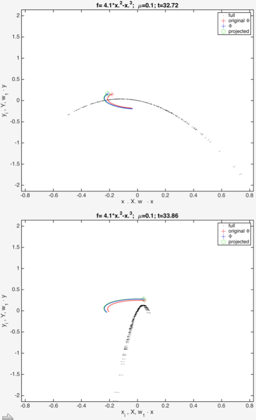
Figure 9: Corrected $\Phi$ As in Fig. 7 adding in blue color the correction using the second order terms in the approximation of $\Phi$ to capture the reduced dynamics.

XIII Numerical Ansatz for Approximating $\Psi$ When $f\left(x\right)=c_{2}x^{2}+c_{3}x^{3}$ and $M$ is Normal and $\lambda_{k}\approx-d$ for $k\geq 2$.

Let’s use the 2nd order nonlinearities of the center manifold (at the bifurcation point) as a guess of the residuals of individual units for small $\lambda_{1}>0$ .

$$x_{i}={\sqrt{N}}V_{i,1}X_{\lambda_{1}}+\underset{k=2}{\overset{N}{\sum}}{\sqrt{N}}V_{i,k}X_{\lambda_{k}}\approx{\sqrt{N}}V_{i,1}X_{\lambda_{1}}+\underset{k=2}{\overset{N}{\sum}}{\sqrt{N}}V_{i,k}c_{2}{\sqrt{N}}\varGamma_{k}^{2\delta_{1,\bullet}}\left(\dfrac{-2\lambda_{k}}{4\lambda_{k}^{2}+9}X_{\lambda_{1}}^{2}+\dfrac{-6}{4\lambda_{k}^{2}+9}X_{\lambda_{1}}Y_{\lambda_{1}}+\dfrac{2\lambda_{k}}{4\lambda_{k}^{2}+9}Y_{\lambda_{1}}^{2}\right)$$

If for $k\geq 2$ ,$\lambda_{k}\approx-d$ then:

$$x_{i}\approx{\sqrt{N}}V_{i,1}X_{\lambda_{1}}+c_{2}\underset{k=2}{\overset{N}{\sum}}{\sqrt{N}}^{2}V_{i,k}\varGamma_{k}^{2\delta_{1,\bullet}}\left(\dfrac{2d}{4d^{2}+9}X_{\lambda_{1}}^{2}+\dfrac{-6}{4d^{2}+9}X_{\lambda_{1}}Y_{\lambda_{1}}+\dfrac{-2d}{4d^{2}+9}Y_{\lambda_{1}}^{2}\right)$$

If $M$ is normal then : $\underset{k=2}{\overset{N}{\sum}}V_{i,k}\varGamma_{k}^{2\delta_{1,\bullet}}=\underset{k=2}{\overset{N}{\sum}}V_{i,k}\underset{\varphi=1}{\overset{N}{\sum}}V_{\varphi,k}V_{\varphi,1}^{2}=\underset{\varphi=1}{\overset{N}{\sum}}V_{\varphi,1}^{2}\left(\delta_{i,\varphi}-V_{i,1}V_{\varphi,1}\right)=V_{i,1}^{2}-V_{i,1}\Gamma_{1}^{2\delta_{1,\bullet}}$.

Since $\left(\sqrt{N}\right)^{2}V_{i,1}\Gamma_{1}^{2\delta_{1,\bullet}}\xrightarrow{N\rightarrow\infty}0$. We get:

$$x_{i} \approx \left(\sqrt{N}\right)V_{i,1}X_{\lambda_{1}}+c_{2}\left(\sqrt{N}\right)^{2}V_{i,1}^{2}\left(\frac{2d}{4d^{2}+9}X_{\lambda_{1}}^{2}+\frac{-6}{4d^{2}+9}X_{\lambda_{1}}Y_{\lambda_{1}}+\frac{-2d}{4d^{2}+9}Y_{\lambda_{1}}^{2}\right)$$

$$y_{i} \approx V_{i,1}\left(\sqrt{N}\right)Y_{\lambda_{1}}+c_{2}\left(\sqrt{N}\right)^{2}V_{i,1}^{2}\left(\frac{-\left(2d^{2}+3\right)}{4d^{2}+9}X_{\lambda_{1}}^{2}+\frac{2d}{4d^{2}+9}X_{\lambda_{1}}Y_{\lambda_{1}}+\frac{-\left(2d^{2}+6\right)}{4d^{2}+9}Y_{\lambda_{1}}^{2}\right)$$

The corrected $\Psi$ is shown in green color in the movie: https://drive.google.com/open?id=1GAUPMhUs04eMjNSbMxjPw8MK2kIGlTZG . Simulation is in red color. Snapshots of the simulation movie are shown in (Fig. 10).

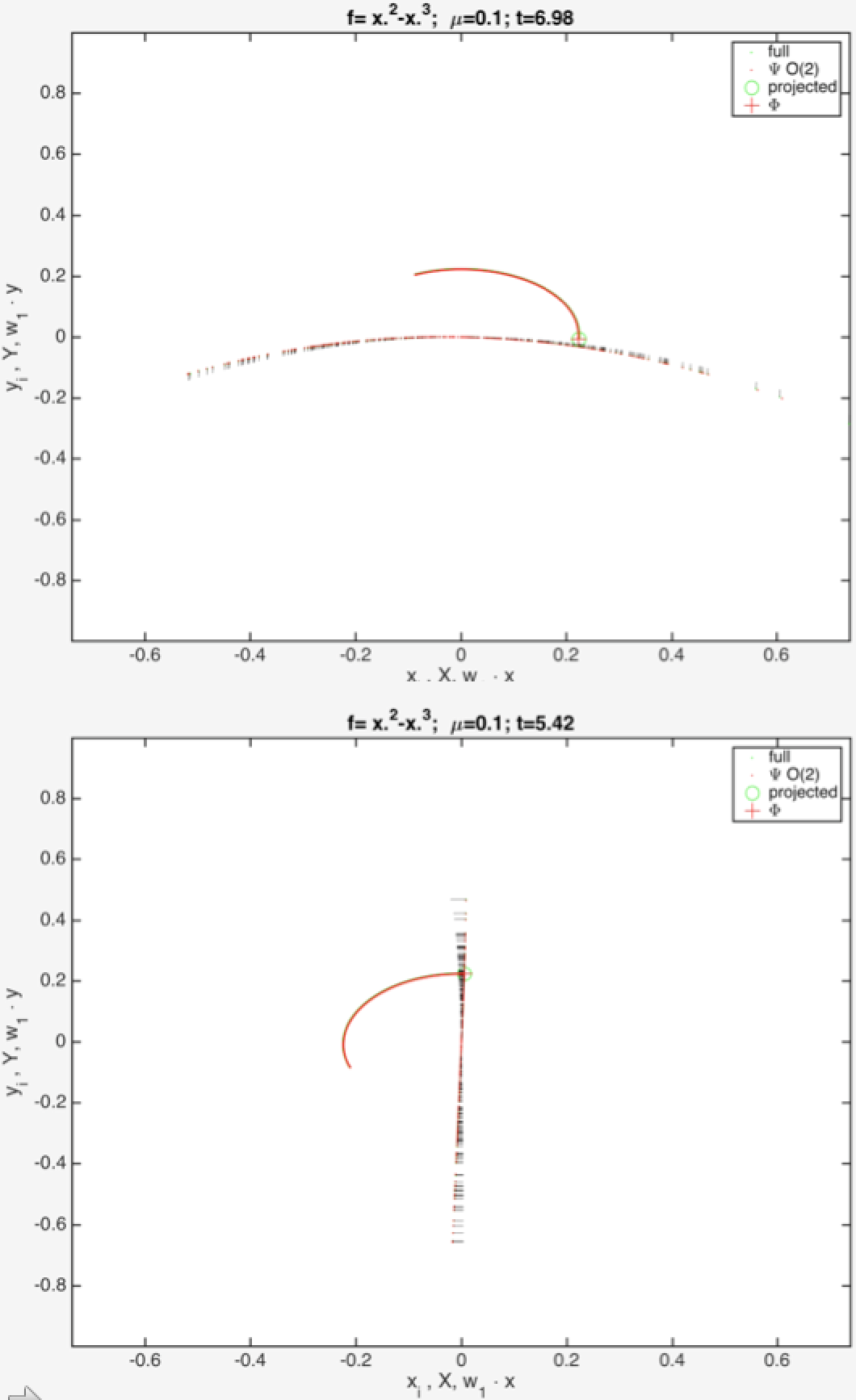
Figure 10: Corrected $\Psi$ with order 2 terms As in Fig. 6 adding in red color the second order terms in the of approximation $\Psi$ to capture the dynamics of individual units from the reduced dynamics.

We see that higher order even nonlinearities also survive on $\Psi$ . https://drive.google.com/open?id=1mb3QK2JGSVxShdKyUA_0bNDhOgSAk_tA. Snapshots of the simulation movie are shown in (Fig. 11).

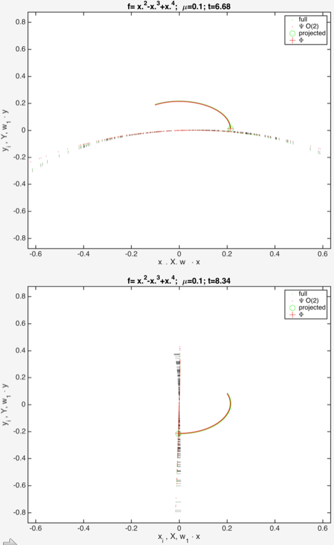
Figure 11: Corrected $\Psi$ with Order 2 Terms Fails to Capture 4th Order Terms As in (Fig. 10) with $f(x)=x^{2}-x^{3}+x^{4}$. Only second order terms of $\Psi$ are not enough.

XIV Numerical Ansatz for Approximating $\Psi$ When $f\left(x\right)=c_{2}x^{2}+c_{3}x^{3}+c_{4}x^{4}+c_{5}x^{5}$ and $M$ is Normal and $\lambda_{k}\approx-d$ for $k\geq 2$.

Assuming that $O(2)*O(2)$ in (27) disappear in the limit and using the highly simplified guess from (28) and adding linear addition $O(2)+O(4)$ we get the approximations on the last movie. In the particular case described here this can intuitively be seen to be an appropriate simplification for $\Lambda\rightarrow\infty$ due to the nonlinearities only surviving on the x layer on $\Phi$ and on the y layer on $\Psi$.

The corrected $\Psi$ is shown in green color in the movie: https://drive.google.com/open?id=1pXFWluButTHG1jReFUm6Rv9J1ihzrNKe. Snapshots of the simulation movie are shown in (Fig. 12).

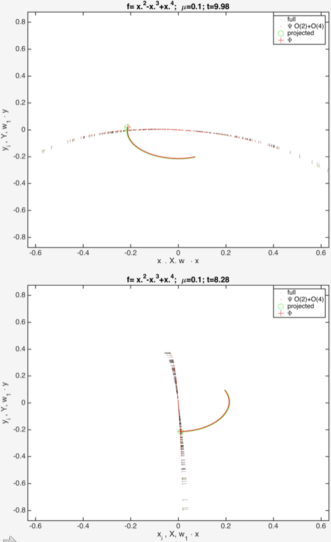
Figure 12: Simplified $\Psi$ Containing Order 2 and 4 Terms As in Fig. 11 but adding terms of order 4 in the approximation of $\Psi$.

XV Complex-Conjugate Pair of Eigenvalues, Normal Matrix

As shown in (Fig. 4), the second-simplest case is to control two complex-conjugate eigenvalues, as they can be controlled by a single parameter, their real part, while leaving their imaginary part unchanged.

We follow the previous section in using $M_{a}$, a normal matrix, as our base connectivity structure. Now we choose a pair of complex-conjugate eigenvalues. The corresponding eigenvectors are also complex conjugate. Choosing as ${e}$ the one corresponding to the eigenvalue with positive imaginary part, the 2D subspace is spanned both by ${e}$ and $\bar{{e}}$, or by ${e}_{R}\equiv\Re{e}$ and ${e}_{I}\equiv\Im{\ e}$. Corollary 2 implies that the whole system bifurcates with 2 pairs of complex conjugate eigenvalues crossing the imaginary axis with frequencies $\dfrac{\sqrt{\omega^{2}+4}\pm\omega}{2}$ .

Following the previous section, and remembering that now the left eigenvector is the complex conjugate of the right eigenvector, ${e}^{\dagger}=\bar{{e}}^{t}$ we define the coarse-grained variable $X$, now complex, as the normalized projection on ${e}$:

$$X\sqrt{\dfrac{N}{2}}=\left({e}_{R}-{e}_{I}i\right)\cdot{x}$$

projection on critical mode, $X=X_{R}+X_{I}i$

Then the linear order approximation of the invariant manifold for the system:

$$\dot{x}_{i} = y_{i}-x_{i}^{\alpha}+\underset{j}{\sum}M_{ij}x_{j}$$

$$\dot{y}_{i} = -x_{i}$$

gives us the linear order of $\Psi$

$${x} \approx \sqrt{\dfrac{N}{2}}\left(X\left({e}_{R}+i{e}_{I}\right)+\bar{X}\left({e}_{R}-i{e}_{I}\right)\right)$$

The naive approximation of $\Psi$ is given by :

$$x = \sqrt{\dfrac{N}{2}}\left(\left(X_{R}+X_{I}i\right)\left(e_{R}+e_{I}i\right)+\left(X_{R}-X_{I}i\right)\left(e_{R}-e_{I}i\right)\right)=\sqrt{2N}\left(X_{R}e_{R}-X_{I}e_{I}\right)$$

$$y = \sqrt{\dfrac{N}{2}}\left(\left(Y_{R}+Y_{I}i\right)\left(e_{R}+e_{I}i\right)+\left(Y_{R}-Y_{I}i\right)\left(e_{R}-e_{I}i\right)\right)=\sqrt{2N}\left(Y_{R}e_{R}-Y_{I}e_{I}\right)$$

Then taking dot product with $\sqrt{\dfrac{N}{2}}e_{R}$ and $-\sqrt{\dfrac{N}{2}}e_{L}$, and ignoring projections other than in $e_{R}$ and $e_{I}$ the system:

$$\dot{x}_{i} = y_{i}-x_{i}^{\alpha}+\underset{j}{\sum}M_{ij}x_{j}$$

$$\dot{y}_{i} = -x_{i}$$

 

gives us :

$$\dot{X}_{R} = Y_{R}+\lambda_{R}X_{R}-\lambda_{I}X_{I}-\sum\sqrt{\dfrac{2}{N}}e_{R,i}\sqrt{2N}^{\alpha}\left(X_{R}e_{R,i}-X_{I,i}e_{I,i}\right)^{\alpha}$$

$$\dot{Y}_{R} = -X_{R}$$

$$\dot{X}_{I} = Y_{I}+\lambda_{I}X_{R}+\lambda_{R}X_{I}-\sum\sqrt{\dfrac{2}{N}}\left(-e_{I,i}\right)\sqrt{2N}^{\alpha}\left(X_{R}e_{R,i}-X_{I,i}e_{I,i}\right)^{\alpha}$$

$$\dot{Y}_{I} = -X_{I}$$

for $\alpha$ odd:

$\sum\sqrt{\dfrac{2}{N}}e_{R,i}\sqrt{2N}^{\alpha}\left(X_{R}e_{R,i}-X_{I,i}e_{I,i}\right)^{\alpha}=\underset{\varphi=0}{\overset{\alpha}{\sum}}\begin{pmatrix}\alpha\\ \varphi\end{pmatrix}\dfrac{1}{N}\sqrt{2N}^{\alpha+1}\underset{i}{\sum}e_{R,i}^{\alpha-\varphi}\left(-e_{I,i}\right)^{\varphi}=$

$X_{R}\underset{\varphi=0}{\overset{\frac{\alpha-1}{2}}{\sum}}\begin{pmatrix}\alpha\\ 2\phi\end{pmatrix}\left(\alpha-2\phi+1\right)!!\left(2\phi\right)!!X_{R}^{\alpha-2\phi-1}X_{I}^{2\phi}=\alpha!!X_{R}\left(X_{R}^{2}+X_{I}^{2}\right)^{\frac{\alpha-1}{2}}$

since $\begin{pmatrix}\alpha\\ 2\phi\end{pmatrix}\left(\alpha-2\phi+1\right)!!\left(2\phi\right)!!=\alpha!!\begin{pmatrix}\frac{\alpha-1}{2}\\ \phi\end{pmatrix}$

similarly $\sum\sqrt{\dfrac{2}{N}}\left(-e_{I,i}\right)\sqrt{2N}^{\alpha}\left(X_{R}e_{R,i}-X_{I,i}e_{I,i}\right)^{\alpha}=\alpha!!X_{I}\left(X_{R}^{2}+X_{I}^{2}\right)^{\frac{\alpha-1}{2}}$

 

So:

$$\dot{X} = Y+\lambda X-\alpha!!\left\|X\right\|^{\alpha-1}X$$

$$\dot{Y} = -X$$

For $\alpha=3$ this is a complex generalized van der Pol equation.

$$\dot{X} = (\lambda-|X|^{2})X+Y$$

$$\dot{Y} = -X$$

Notice the $X$ equation is now a Hopf bifurcation normal form in a single complex variable, where ${Imag}(\lambda)$ is the rotational frequency in the $X$ complex plane, and ${Real}(\lambda)$ is the control parameter, while the whole $XY$ plane equation uses the same ${Real}(\lambda)$ as a control parameter for a Hopf bifurcation in the real $XY$ plane. Thus this equation contains 2 distinct frequencies, $\omega=1$ from the base equation, and $\omega={Imag}(\lambda)$, the frequency of the eigenvector, from the complex $X$ equation, and both cross the threshold of stability at the same time. Therefore, in this collective mode, a codimension-2 transition becomes generic, and the system in principle can bifurcate directly from a fixed point onto a torus. In this sense it is similar to a Takens-Bogdanoff normal form, only that it has two distinct and independent frequencies.

Thus the reduced equations are non-generic with respect to perturbations of the individual units in the full system in two ways: first, all even terms are destroyed, and second it can undergo a direct transition from a fixed point to a torus.

XVI Conclusion

We have proposed a statistical center manifold reduction technique based on the three foundational center manifold theorems: existence, stability, and approximation Kelley (1967); Carr (2012). Utilizing these theorems we have constructed two key operators. The first operator $\Phi$ connects the statistics of the vector field in the full-dimensional space to the statistics of the reduced vector field in the low-dimensional space. The second operator $\Psi$ lifts the statistical properties of the trajectories produced by these reduced vector fields to the trajectories evolved by the original vector fields. For any given system, these two operators are sufficient to verify that our center manifold dimensionality reduction approach is well defined (the diagram in Fig. 3 commutes).

In this paper, we have considered a specific example of a simple network of randomly connected, spontaneous oscillators. We have shown that our center manifold dimensionality reduction approach is well defined, successfully capturing the statistical properties of the individual units in the full system. The operators $\Phi$ and $\Psi$ depend crucially on the structure of the eigenvectors (through the random variables $\Gamma$’s). While we now know quite a lot about the statistical nature of the eigenvalues of random matrices Tao (2008), little is known about the statistical structure of the eigenvectors of these matrices Chalker (1998); Tao (2012); O’Rourke (2016). In the considered example, the reduction operator $\Phi$ coarse grains out the even nonlinearities present in the full system. But even though the even nonlinearities are coarse-grained out, we have found that they can still leak to higher order odd nonlinearities, which can have drastic effects on the dynamics as a whole, and for example, create a subcritical Hopf bifurcation from subunits of supercritical Hopf bifurcations. Moreover, using simplifying assumptions in the approximation theorem, we were able to construct a lift operator $\Psi$ for higher order nonlinearities. This lift operator has interesting properties like in the limit of $d\rightarrow\inf$, the even nonlinearities survive only in the y layer and the odd nonlinearities vanish entirely.

We have explored several other systems and it appears that the property of even nonlinearities being coarse-grained out in the reduced dynamics generally holds for a class of similar systems although the exact nature of this class is not yet clear. Furthermore, it should be easily to generalize to other structures such as sparsity by calculating new values for the $\Gamma$’s. Both these subjects should be a target of future research.

References

- Adelmeyer (1999) Adelmeyer M. Topics in bifurcation theory and applications. World Scientific Publishing Company; 1999 Jan 22.
- Alonso (2014) Alonso LM, Proekt A, Schwartz TH, Pryor KO, Cecchi GA, Magnasco MO. Dynamical criticality during induction of anesthesia in human ECoG recordings. Frontiers in neural circuits. 2014 Mar 25;8:20.
- Anderson (2010) Anderson GW, Guionnet A, Zeitouni O. An introduction to random matrices, volume 118 of Cambridge Studies in Advanced Mathematics.
- (4) Andronov AA, Vitt AA, Khaikin SE. Theory of Oscillators: Adiwes International Series in Physics. Elsevier; 2013 Oct 22.
- Arieli (1996) Arieli A, Sterkin A, Grinvald A, Aertsen AD. Dynamics of ongoing activity: explanation of the large variability in evoked cortical responses. Science. 1996 Sep 27;273(5283):1868-71.
- Beggs (2003) Beggs JM, Plenz D. Neuronal avalanches in neocortical circuits. Journal of neuroscience. 2003 Dec 3;23(35):11167-77.
- Beggs (2012) Beggs JM, Timme N. Being critical of criticality in the brain. Frontiers in physiology. 2012 Jun 7;3:163.
- Belkin (2003) Belkin M, Niyogi P. Laplacian eigenmaps for dimensionality reduction and data representation. Neural computation. 2003 Jun 1;15(6):1373-96.
- Bienenstock (1998) Bienenstock E, Lehmann D. Regulated criticality in the brain?. Advances in complex systems. 1998 Dec;1(04):361-84.
- Brauer (1952) Brauer A. Limits for the characteristic roots of a matrix. IV: Applications to stochastic matrices. Duke Mathematical Journal. 1952 Mar;19(1):75-91.
- Camalet (2000) Camalet S, Duke T, Julicher F, Prost J. Auditory sensitivity provided by self-tuned critical oscillations of hair cells. Proceedings of the National Academy of Sciences. 2000 Mar 28;97(7):3183-8.
- Carlsson (2009) Carlsson G. Topology and data. Bulletin of the American Mathematical Society. 2009;46(2):255-308.
- Carr (2012) Carr J. Applications of centre manifold theory. Springer Science and Business Media; 2012 Dec 6.
- Chalker (1998) Chalker JT, Mehlig B. Eigenvector statistics in non-Hermitian random matrix ensembles. Physical review letters. 1998 Oct 19;81(16):3367.
- Chialvo (2010) Chialvo DR. Emergent complex neural dynamics. Nature physics. 2010 Oct;6(10):744.
- Choe (1998) Choe Y, Magnasco MO, Hudspeth AJ. A model for amplification of hair-bundle motion by cyclical binding of Ca2+ to mechanoelectrical-transduction channels. Proceedings of the National Academy of Sciences. 1998 Dec 22;95(26):15321-6.
- Churchland (2012) Churchland MM, Cunningham JP, Kaufman MT, Foster JD, Nuyujukian P, Ryu SI, Shenoy KV. Neural population dynamics during reaching. Nature. 2012 Jul;487(7405):51.
- Dasgupta (2008) Dasgupta S, Freund Y. Random projection trees and low dimensional manifolds. InSTOC 2008 May 17 (Vol. 8, pp. 537-546).
- Donoho (2003) Donoho DL, Grimes C. Hessian eigenmaps: Locally linear embedding techniques for high-dimensional data. Proceedings of the National Academy of Sciences. 2003 May 13;100(10):5591-6.
- Dulac (1903) Dulac H. Recherches sur les points singuliers des équations différentielles. Gauthier-Villars; 1903.
- Duke (2003) Duke T, Julicher F. Active traveling wave in the cochlea. Physical review letters. 2003 Apr 16;90(15):158101.
- Eguíluz (2000) Eguíluz VM, Ospeck M, Choe Y, Hudspeth AJ, Magnasco MO. Essential nonlinearities in hearing. Physical Review Letters. 2000 May 29;84(22):5232.
- Eguíluz (2005) Eguíluz VM, Chialvo DR, Cecchi GA, Baliki M, Apkarian AV. Scale-free brain functional networks. Physical review letters. 2005 Jan 6;94(1):018102.
- Engelken (2016) Engelken R, Farkhooi F, Hansel D, van Vreeswijk C, Wolf F. A reanalysis of “Two types of asynchronous activity in networks of excitatory and inhibitory spiking neurons”. F1000Research. 2016;5.
- Fox (2005) Fox MD, Snyder AZ, Vincent JL, Corbetta M, Van Essen DC, Raichle ME. The human brain is intrinsically organized into dynamic, anticorrelated functional networks. Proceedings of the National Academy of Sciences. 2005 Jul 5;102(27):9673-8.
- Fox (2006) Fox MD, Corbetta M, Snyder AZ, Vincent JL, Raichle ME. Spontaneous neuronal activity distinguishes human dorsal and ventral attention systems. Proceedings of the National Academy of Sciences. 2006 Jun 27;103(26):10046-51.
- Fraiman (2009) Fraiman D, Balenzuela P, Foss J, Chialvo DR. Ising-like dynamics in large-scale functional brain networks. Physical Review E. 2009 Jun 23;79(6):061922.
- Freeman (2005) Freeman WJ, Holmes MD. Metastability, instability, and state transition in neocortex. Neural Networks. 2005 Aug 31;18(5):497-504.
- Freire (1988) Freire E, Gamero E, Ponce E, Franquelo LG. An algorithm for symbolic computation of center manifolds. InInternational Symposium on Symbolic and Algebraic Computation 1988 Jul 4 (pp. 218-230). Springer, Berlin, Heidelberg.
- Genovese (2012) Genovese CR, Perone-Pacifico M, Verdinelli I, Wasserman L. Manifold estimation and singular deconvolution under Hausdorff loss. The Annals of Statistics. 2012;40(2):941-63.
- Géron (2017) Géron A. Hands-on machine learning with Scikit-Learn and TensorFlow: concepts, tools, and techniques to build intelligent systems. " O’Reilly Media, Inc."; 2017 Mar 13.
- Gireesh (2008) Gireesh ED, Plenz D. Neuronal avalanches organize as nested theta-and beta/gamma-oscillations during development of cortical layer 2/3. Proceedings of the National Academy of Sciences. 2008 May 27;105(21):7576-81.
- Grobman (1959) Grobman DM. Homeomorphism of systems of differential equations. Doklady Akademii Nauk SSSR. 1959 Jan 1;128(5):880-1.
- Guckenheimer (2013) Guckenheimer J, Holmes P. Nonlinear oscillations, dynamical systems, and bifurcations of vector fields. Springer Science and Business Media; 2013 Nov 21.
- Hansel (1997) Hansel D, Sompolinsky H. 13 Modeling Feature Selectivity in Local Cortical Circuits.
- Harish (2015) Harish O, Hansel D. Asynchronous rate chaos in spiking neuronal circuits. PLoS computational biology. 2015 Jul 31;11(7):e1004266.
- (37) Hartman P. A lemma in the theory of structural stability of differential equations. Proceedings of the American Mathematical Society. 1960;11(4):610-20.
- (38) Hartman P. On local homeomorphisms of Euclidean spaces. Bol. Soc. Mat. Mexicana. 1960 Oct;5(2):220-41.
- Hastie (1989) Hastie T, Stuetzle W. Principal curves. Journal of the American Statistical Association. 1989 Jun 1;84(406):502-16.
- (40) Hayton K, Moirogiannis D, Magnasco M (2018) Adaptive scales of integration and response latencies in a critically-balanced model of the primary visual cortex. PLoS ONE 13(4): e0196566.
- (41) Hayton K, Moirogiannis D, Magnasco M. A Nonhyperbolic Toy Model of Cochlear Dynamics. arXiv preprint arXiv:1807.00764. 2018 Jul 2.
- Hopf (1942) Hopf E. Abzweigung einer periodischen Lösung von einer stationären Lösung eines Differentialsystems. Ber. Math.-Phys. Kl Sächs. Akad. Wiss. Leipzig. 1942 Jan;94:1-22.
- Hoppensteadt (2012) Hoppensteadt FC, Izhikevich EM. Weakly connected neural networks. Springer Science and Business Media; 2012 Dec 6.
- Ioos (1999) Ioos G, Adelmeyer M. Topics in Bifurcation Theory and Applications. Advanced Series in Nonlinear Dynamics. World Scientific, 2nd edition, 1999
- (45) Izhikevich EM. Dynamical systems in neuroscience. MIT press; 2007.
- (46) Izhikevich EM. Equilibrium. Scholarpedia. 2007 Oct 9;2(10):2014.
- Kadmon (2015) Kadmon J, Sompolinsky H. Transition to chaos in random neuronal networks. Physical Review X. 2015 Nov 19;5(4):041030.
- (48) Kanders K, Lorimer T, Stoop R. Avalanche and edge-of-chaos criticality do not necessarily co-occur in neural networks. Chaos: An Interdisciplinary Journal of Nonlinear Science. 2017 Apr;27(4):047408.
- (49) Kanders K, Lorimer T, Gomez F, Stoop R. Frequency sensitivity in mammalian hearing from a fundamental nonlinear physics model of the inner ear. Scientific Reports. 2017 Aug 30;7(1):9931.
- Kégl (2000) Kégl B, Krzyzak A, Linder T, Zeger K. Learning and design of principal curves. IEEE transactions on pattern analysis and machine intelligence. 2000 Mar;22(3):281-97.
- Kelley (1967) Kelley A. The stable, center-stable, center, center-unstable, unstable manifolds. Journal of Differential Equations. 1967 Oct 1;3(4):546-70.
- Kenet (2003) Kenet T, Bibitchkov D, Tsodyks M, Grinvald A, Arieli A. Spontaneously emerging cortical representations of visual attributes. Nature. 2003 Oct;425(6961):954.
- Kern (2003) Kern A, Stoop R. Essential role of couplings between hearing nonlinearities. Physical Review Letters. 2003 Sep 19;91(12):128101.
- Kambhatla (1994) Kambhatla N, Leen TK. Fast non-linear dimension reduction. InAdvances in neural information processing systems 1994 (pp. 152-159).
- Kitzbichler (2009) Kitzbichler MG, Smith ML, Christensen SR, Bullmore E. Broadband criticality of human brain network synchronization. PLoS computational biology. 2009 Mar 20;5(3):e1000314.
- Kuznetsov (2013) Kuznetsov YA. Elements of applied bifurcation theory. Springer Science and Business Media; 2013 Mar 9.
- Lalazar (2016) Lalazar H, Abbott LF, Vaadia E. Tuning curves for arm posture control in motor cortex are consistent with random connectivity. PLoS computational biology. 2016 May 25;12(5):e1004910.
- Landau (2016) Landau ID, Egger R, Dercksen VJ, Oberlaender M, Sompolinsky H. The impact of structural heterogeneity on excitation-inhibition balance in cortical networks. Neuron. 2016 Dec 7;92(5):1106-21.
- Levina (2007) Levina A, Herrmann JM, Geisel T. Dynamical synapses causing self-organized criticality in neural networks. Nature physics. 2007 Dec;3(12):857.
- Machens (2005) Machens CK, Romo R, Brody CD. Flexible control of mutual inhibition: a neural model of two-interval discrimination. Science. 2005 Feb 18;307(5712):1121-4.
- Magnasco (2003) Magnasco MO. A wave traveling over a Hopf instability shapes the cochlear tuning curve. Physical review letters. 2003 Feb 4;90(5):058101.
- Magnasco (2009) Magnasco MO, Piro O, Cecchi GA. Self-tuned critical anti-Hebbian networks. Physical review letters. 2009 Jun 22;102(25):258102.
- Moirogiannis (2017) Moirogiannis D, Piro O, Magnasco MO. Renormalization of Collective Modes in Large-Scale Neural Dynamics. Journal of Statistical Physics. 2017 May 1;167(3-4):543-58.
- Mora (2011) Mora T, Bialek W. Are biological systems poised at criticality?. Journal of Statistical Physics. 2011 Jul 1;144(2):268-302.
- Narayanan (2009) Narayanan H, Niyogi P. On the Sample Complexity of Learning Smooth Cuts on a Manifold. InCOLT 2009 Jun.
- Nauhaus (2009) Nauhaus I, Busse L, Carandini M, Ringach DL. Stimulus contrast modulates functional connectivity in visual cortex. Nature neuroscience. 2009 Jan 1;12(1):70-6.
- Niyogi (2008) Niyogi P, Smale S, Weinberger S. Finding the homology of submanifolds with high confidence from random samples. Discrete and Computational Geometry. 2008 Mar 1;39(1-3):419-41.
- O’Rourke (2016) O’Rourke S, Vu V, Wang K. Eigenvectors of random matrices: a survey. Journal of Combinatorial Theory, Series A. 2016 Nov 1;144:361-442.
- Ostojic (2014) Ostojic S. Two types of asynchronous activity in networks of excitatory and inhibitory spiking neurons. Nature neuroscience. 2014 Apr;17(4):594.
- Perrault-Jones (2012) Perrault-Joncas D, Meila M. Metric learning and manifolds: Preserving the intrinsic geometry. Preprint Department of Statistics, University of Washington. 2012.
- Petersen (2003) Petersen CC, Hahn TT, Mehta M, Grinvald A, Sakmann B. Interaction of sensory responses with spontaneous depolarization in layer 2/3 barrel cortex. Proceedings of the National Academy of Sciences. 2003 Nov 11;100(23):13638-43.
- Poincarè (1893) Poincarè H. Les méthodes nouvelles de la mécanique céleste: Méthodes de MM. Newcomb, Glydén, Lindstedt et Bohlin. 1893. Gauthier-Villars it fils; 1893.
- Rajan (2016) Rajan K, Harvey CD, Tank DW. Recurrent network models of sequence generation and memory. Neuron. 2016 Apr 6;90(1):128-42.
- Roweis (2000) Roweis ST, Saul LK. Nonlinear dimensionality reduction by locally linear embedding. science. 2000 Dec 22;290(5500):2323-6.
- Smola (2001) Smola AJ, Mika S, Schölkopf B, Williamson RC. Regularized principal manifolds. Journal of Machine Learning Research. 2001;1(Jun):179-209.
- Sompolinsky (1998) Sompolinsky H, Crisanti A, Sommers HJ. Chaos in random neural networks. Physical review letters. 1988 Jul 18;61(3):259.
- Sompolinsky (2014) Sompolinsky, H.: Computational neuroscience: beyond the local circuit. Curr. Opin. Neurobiol. 25, 1–6 (2014)
- Seung (1998) Seung HS. Continuous attractors and oculomotor control. Neural Networks. 1998 Nov 30;11(7):1253-8.
- Seung (2000) Seung HS, Lee DD, Reis BY, Tank DW. Stability of the memory of eye position in a recurrent network of conductance-based model neurons. Neuron. 2000 Apr 30;26(1):259-71.
- Shnol (2007) Shnol EE. Stability of equilibria. Scholarpedia. 2007 Mar 15;2(3):2770.
- Silva (1998) da Silva L, Papa AR, de Souza AC. Criticality in a simple model for brain functioning. Physics Letters A. 1998 Jun 8;242(6):343-8.
- Solovey (2012) Solovey G, Miller KJ, Ojemann J, Magnasco MO, Cecchi GA. Self-regulated dynamical criticality in human ECoG. Frontiers in integrative neuroscience. 2012 Jul 19;6:44.
- Solovey (2015) Solovey G, Alonso LM, Yanagawa T, Fujii N, Magnasco MO, Cecchi GA, Proekt A. Loss of consciousness is associated with stabilization of cortical activity. Journal of Neuroscience. 2015 Jul 29;35(30):10866-77.
- Stern (2014) Stern M, Sompolinsky H, Abbott LF. Dynamics of random neural networks with bistable units. Physical Review E. 2014 Dec 16;90(6):062710.
- Tao (2008) Tao T, Vu V. Random matrices: the circular law. Communications in Contemporary Mathematics. 2008 Apr;10(02):261-307.
- Tao (2012) Tao T, Vu V. Random matrices: Universal properties of eigenvectors. Random Matrices: Theory and Applications. 2012 Jan;1(01):1150001.
- Tenenbaum (2000) Tenenbaum JB, De Silva V, Langford JC. A global geometric framework for nonlinear dimensionality reduction. science. 2000 Dec 22;290(5500):2319-23.
- Tsodyks (1999) Tsodyks M, Kenet T, Grinvald A, Arieli A. Linking spontaneous activity of single cortical neurons and the underlying functional architecture. Science. 1999 Dec 3;286(5446):1943-6.
- Weinberger (2006) Weinberger KQ, Saul LK. Unsupervised learning of image manifolds by semidefinite programming. International journal of computer vision. 2006 Oct 1;70(1):77-90.
- Wiggins (2003) Wiggins S. Introduction to applied nonlinear dynamical systems and chaos. Springer Science and Business Media; 2003 Oct 1.
- Yan (2012) Yan XH, Magnasco MO. Input-dependent wave attenuation in a critically-balanced model of cortex. PloS one. 2012 Jul 25;7(7):e41419.