Dual-Time Smoothed Particle Hydrodynamics for Incompressible Fluid Simulation

Abstract

In this paper we propose a dual-time stepping scheme for the Smoothed Particle Hydrodynamics (SPH) method. Dual-time stepping has been used in the context of other numerical methods for the simulation of incompressible fluid flows. Here we provide a scheme that combines the entropically damped artificial compressibility (EDAC) along with dual-time stepping. The method is accurate, robust, and demonstrates up to seven times better performance than the standard weakly-compressible formulation. We demonstrate several benchmarks showing the applicability of the scheme. In addition, we provide a completely open source implementation and a reproducible manuscript.

1 Introduction

The Smoothed Particle Hydrodynamics (SPH) method originated with the work of Gingold and Monaghan [1], and Lucy [2] as a method to simulate astrophysical problems. The method is grid-free and Lagrangian in nature. It has since become a very general purpose technique and applied to a variety of problems including incompressible fluid flow[3, 4, 5], solid mechanics[6], and fluid-structure interaction [7, 8].

There are several SPH schemes for simulating incompressible and weakly compressible fluid flows. The original weakly compressible SPH scheme (WCSPH) was proposed by Monaghan [3]. This scheme treats the fluid as weakly compressible with an artificial sound speed and a stiff equation of state. This allows the scheme to utilize a hyperbolic system of equations and integrate them in time. There are many significant variants of this scheme including a Transport Velocity Formulation (TVF) [9] which introduces a transport velocity to ensure particle homogeneity. The original WCSPH and their derivatives generally suffer from a large amount of pressure oscillations and the $\delta$-SPH scheme [10, 11] reduces these oscillations by introducing a dissipation into the continuity equation. Similarly, an Entropically Damped Artificial Compressibility SPH scheme (EDAC-SPH)[12] has been proposed which introduces entropy by diffusing the pressure. This approach is quite similar to the $\delta$-SPH scheme and both schemes produce superior pressure distributions. All of these schemes employ an artificial sound speed and this places severe time step limitations due to stability considerations.

Cummins and Rudman [4] proposed a family of projection based schemes for incompressible fluids. Shao and Lo [5] and Hu and Adams [13] proposed incompressible SPH (ISPH) schemes which satisfy incompressibility by solving a pressure-Poisson equation. These approaches eliminate the need for evolving the pressure at the sound speed and this significantly increases the allowed time steps. The difficulty with the projection and incompressible schemes is the requirement to solve a linear system of equations which can be time consuming and involved. Recently, a Predictive-Corrective ISPH (PCISPH) [14] has been proposed for use in the graphics community for rapid simulation of incompressible fluids. A more accurate and efficient scheme has been proposed called the Implicit-Incompressible SPH (IISPH) [15]. The IISPH is matrix-free, and very efficient. It has been shown to be close to an order of magnitude faster than traditional schemes. However, the IISPH can be more involved to implement than many of the traditional WCSPH-based schemes. Recently, another fast and matrix-free implementation of the ISPH method has been proposed [16].

In this paper we propose a new scheme for weakly-compressible fluid flows. Our paper takes inspiration from the Artificial Compressiblility-based Incompressible SPH (ACISPH) scheme proposed by Rouzbahani and Hejranfar [17]. Our scheme uses a different formulation that is also very efficient. The original scheme was not noted in particular for its efficiency. We propose an original derivation and suggest many improvements that make the proposed scheme efficient. The performance is significantly better than that of the traditional WCSPH schemes and comparable to that of the ISPH schemes without sacrificing any accuracy or being unduly hard to implement. Our approach employs the classic artificial compressibility of Chorin [18] in a dual-time stepped framework. We call the resulting scheme, DTSPH for Dual-Time stepped SPH.

Fatehi et al. [19] propose density-based dual-timestepping schemes for the SPH method. They propose two different formulations in order to update the pressure in pseudo-time. They perform an accurate discretization of the derivatives. While their method is in principle similar to the present work, it does not demonstrate any significant performance advantage over the traditional WCSPH schemes. Moreover, they do not demonstrate their method with any free-surface problems. Our proposed implementation and method is however significantly faster than the WCSPH scheme and has been demonstrated to work well for free-surface and three-dimensional problems. Zhang et al. [20] on the other hand propose a dual-criteria timestepping strategy that is quite different from the method proposed here or in [19, 17]. They use an “acoustic timestep” to relax the pressure and an “advective timestep” to update the verlet lists used for neighbor computation. This optimization results in a performance improvement without significant complexity albeit at the cost of increased memory. The present method demonstrates much improved performance and does not involve a significant memory penalty.

The new scheme is designed to be implemented as an extension of the classic weakly-compressible schemes. The advantage of this is that these are relatively easy to implement, boundary conditions may be easily enforced, and there are several well-established schemes that may be used. Although we have not done so in this manuscript, it is important to note that this approach may also be employed for solid mechanics problems where the artificial speed of sound is usually very large.

The new scheme can be adapted to any WCSPH formulation which uses a density or pressure evolution equation based on a continuity equation. We demonstrate the scheme with the EDAC scheme [12]. We note that it can be easily applied to other schemes like the $\delta$-SPH. We show how our scheme can be used to obtain steady state solutions, although this is not particular to the new scheme and can be easily performed for a variety of other schemes. Obtaining steady state solutions in the context of SPH simulations is useful in different contexts. For example, in the case of the impulsively started flow past a complex geometry, an initial potential flow solution is useful and this may be easily obtained using this approach.

In this manuscript we provide a new formulation as compared to the work of [17], explore several important details for the implementation of the scheme, and more importantly provide a high-performance, open source implementation of the scheme. Our implementation uses the open source PySPH framework [21, 22] and all the code related to the manuscript is available at https://gitlab.com/pypr/dtsph. In order to facilitate reproducible research, this entire manuscript is completely reproducible and every figure in this paper is automatically generated using automan [23].

In the next section we discuss the proposed DTSPH scheme in a general setting and then discuss the SPH discretization. We briefly discuss the stability requirements of the scheme. We show how the resulting scheme is efficient and then proceed to simulate various standard benchmark problems. We perform comparisons with the TVF [9], the $\delta$-SPH scheme [10], and the EDAC scheme [12] where relevant to demonstrate the accuracy and efficiency of the proposed scheme.

2 The dual-time SPH method

In dual-time stepping schemes, a new time dimension called the “dual-time”, denoted by the variable $\tau$, is introduced. We have the following important considerations to keep in mind. If $\mathbf{r}$ is the position vector of a particle, then the real velocity of the particle is defined as, $\mathbf{V}=\frac{d\mathbf{r}}{dt}$. On the other hand, if the particle were to move in pseudo-time, we define the velocity in pseudo-time as $\mathbf{\tilde{V}}=\frac{d\mathbf{r}}{d\tau}$.

If we consider a property of the particle, $p$, then we can define a material derivative in pseudo-time as,

$$\frac{dp}{d\tau}=\frac{\partial p}{\partial\tau}+\mathbf{\tilde{V}}\cdot\text{grad}(p).$$ (1)

The ACISPH formulation [17] uses a non-dimensionalized form of the equation,

$$\frac{1}{\beta^{2}}\frac{\partial p^{*}}{\partial\tau^{*}}+\text{div}(\mathbf{V^{*}})=0.$$ (2)

Here we use a star for the non-dimensional terms. By assuming that $p=(\rho-\rho_{0})c^{2}$ where $c$ is an artificial sound speed and $\rho_{0}$ is a reference density, the above can be written in a dimensional form as,

$$\frac{\partial p}{\partial\tau}=-\rho c^{2}\text{div}(\mathbf{V}).$$ (3)

By rewriting the non-dimensional form in equation (2) with suitable dimensional quantities, it is easy to see that $\beta=1/M$ where $M=V_{ref}/c$ is the Mach number of the reference speed of the flow, $V_{ref}$.

If we move the particles in pseudo-time, we introduce a material derivative to get,

$$\frac{dp}{d\tau}=\mathbf{\tilde{V}}\cdot\text{grad}(p)-\rho c^{2}\text{div}(\mathbf{V}).$$ (4)

With the EDAC formulation [12], the pressure evolution equation also includes a diffusive term and we get,

$$\frac{dp}{d\tau}=\mathbf{\tilde{V}}\cdot\text{grad}(p)-\rho c^{2}\text{div}(\mathbf{V})+\nu_{e}\nabla^{2}p,$$ (5)

where $\nu_{e}$ is an artificial viscosity parameter which is typically chosen as,

$$\nu_{e}=\frac{hc}{16}.$$ (6)

Here $h$ is the SPH kernel radius. In the above, we have assumed that the particles move in pseudo-time. In later sections, we show that it is computationally efficient to not move the particles in pseudo-time. This results in a simpler equation for the pressure evolution without a time derivative as,

$$\frac{\partial p}{\partial\tau}=-\rho c^{2}\text{div}(\mathbf{V})+\nu_{e}\nabla^{2}p.$$ (7)

The momentum equation can be written similarly by adding a time derivative of velocity in pseudo-time,

$$\frac{\partial\mathbf{V}}{\partial\tau}+\frac{d\mathbf{V}}{dt}=-\frac{1}{\rho}\text{grad}(p)+\nu\nabla^{2}\mathbf{V}+\mathbf{f},$$ (8)

where $\nu$ is the kinematic viscosity of the fluid and $\mathbf{f}$ is the body force. Again, if we choose to move the particles in pseudo-time, we can write this in terms of a material derivative in pseudo-time as,

$$\frac{d\mathbf{V}}{d\tau}+\frac{d\mathbf{V}}{dt}=\mathbf{\tilde{V}}\cdot\text{grad}(\mathbf{V})-\frac{1}{\rho}\text{grad}(p)+\nu\nabla^{2}\mathbf{V}+\mathbf{f}.$$ (9)

Note the key difference here from what is proposed in [17] is that they have used $\mathbf{V}$ where they should have only used $\mathbf{\tilde{V}}$.

There are two possible approaches we can choose for implementation:

• Move particles in real time and pseudo-time and use the equations (4) and (9). Note that when using the EDAC formulation we would add the pressure diffusion term as shown in the right hand side of (5).

• Move the particles only in real time and use equations (3) (or (7) in the case of the EDAC scheme) and (8).

We discuss these two approaches next.

2.1 Moving particles in pseudo-time

In this section we show how the above equations are integrated in real time and pseudo-time. The following equations apply to each particle, $i$. We suppress the subscript $i$ in the following to simplify the notation. We use the index $k$ to denote pseudo-time iterations and $n$ for the real time. Before iterating in pseudo time the particles are updated to a guessed new state ($k=0$) for the next real time ($n+1$) using,

$$\mathbf{V}^{k=0}=\mathbf{V}^{n}+\Delta t{\left(\frac{d\mathbf{V}}{dt}\right)}^{n},$$ (10)

$$\mathbf{r}^{k=0}=\mathbf{r}^{n}+\Delta t\mathbf{V}^{n}+\frac{\Delta t^{2}}{2}{\left(\frac{d\mathbf{V}}{dt}\right)}^{n},$$ (11)

where ${(\frac{d\mathbf{V}}{dt})}^{n}$ is given by the momentum equation (8) without the partial derivative of velocity in pseudo time (i.e. considering $\frac{\partial\mathbf{V}}{\partial\tau}=0$). Then the integration in pseudo time proceeds in the following fashion, with $\mathbf{\tilde{V}}^{k=0}=0$ as the starting value,

$$\mathbf{r}^{k+1/2}=\mathbf{r}^{k}+\frac{1}{2}\Delta\tau\mathbf{\tilde{V}}^{k},$$ (12)

$$p^{k+1/2}=p^{k}+\frac{1}{2}\Delta\tau{\left(\frac{dp}{d\tau}\right)}^{k},$$ (13)

$$\mathbf{V}^{k+1}=\mathbf{V}^{k}+\Delta\tau{\left(\frac{d\mathbf{V}}{d\tau}\right)}^{k+1/2},$$ (14)

$$\mathbf{r}^{k+1}=\mathbf{r}^{k+1/2}+\frac{1}{2}\Delta\tau\mathbf{\tilde{V}}^{k+1},$$ (15)

$$p^{k+1}=p^{k+1/2}+\frac{1}{2}\Delta\tau{\left(\frac{dp}{d\tau}\right)}^{k+1/2}.$$ (16)

In addition to these we have,

$$\mathbf{\tilde{V}}^{k+1}={\left(\frac{d\mathbf{V}}{d\tau}\right)}^{k+1/2}\Delta t.$$ (17)

This is to ensure consistency of the motion. A detailed proof for equation (17) is provided in the appendix at the end of this manuscript.

We need an expression for the term $\frac{d\mathbf{V}}{dt}$ in the momentum equation (9). We obtain this using an implicit three-point backward difference scheme to discretize the real-time derivative,

$${\left(\frac{d\mathbf{V}}{dt}\right)}^{n+1}=\frac{3\mathbf{V}^{n+1}-4\mathbf{V}^{n}+\mathbf{V}^{n-1}}{2\Delta t}+{O(\Delta t)}^{2}.$$ (18)

Substitute $\mathbf{V}^{k+1}$ instead of $\mathbf{V}^{n+1}$ in (18) and add and subtract the term $3\mathbf{V}^{k}$ in the numerator and rearrange terms to get,

$${\left(\frac{d\mathbf{V}}{dt}\right)}^{n+1}=\frac{3\Delta\tau}{2\Delta t}{\left(\frac{d\mathbf{V}}{d\tau}\right)}^{k+1/2}+\frac{3\mathbf{V}^{k}-4\mathbf{V}^{n}+\mathbf{V}^{n-1}}{2\Delta t}+{O(\Delta t)}^{2}.$$ (19)

If we use equation (9), we can rewrite the above as,

$$\begin{split}\left(\frac{d\mathbf{V}}{d\tau}\right)^{k+1/2}\approx&\left\{\mathbf{\tilde{V}}\cdot\text{grad}(\mathbf{V})-\frac{1}{\rho}\text{grad}(p)+\nu\nabla^{2}\mathbf{V}+\mathbf{f}\right.\\ &\left.-\frac{(3\mathbf{V}^{k}-4\mathbf{V}^{n}+\mathbf{V}^{n-1})}{2\Delta t}\right\}\left(\frac{2\Delta t}{2\Delta t+3\Delta\tau}\right).\end{split}$$ (20)

We may now discretize the right hand side using SPH and find the acceleration to the velocity in pseudo-time. This is done in section 3.

2.2 Fixed particles in pseudo-time

In this section we consider the case where the particles are not moved in pseudo-time. In this case, we can perform the integration as follows,

$$p^{k+1/2}=p^{k}+\frac{1}{2}\Delta\tau{\left(\frac{\partial p}{\partial\tau}\right)}^{k},$$ (21)

$$\mathbf{V}^{k+1}=\mathbf{V}^{k}+\Delta\tau{\left(\frac{\partial\mathbf{V}}{\partial\tau}\right)}^{k+1/2},$$ (22)

$$p^{k+1}=p^{k+1/2}+\frac{1}{2}\Delta\tau{\left(\frac{\partial p}{\partial\tau}\right)}^{k+1/2}.$$ (23)

Further, starting from equation (22), the equation corresponding to (19) becomes,

$${\left(\frac{d\mathbf{V}}{dt}\right)}^{n+1}=\frac{3\Delta\tau}{2\Delta t}{\left(\frac{\partial\mathbf{V}}{\partial\tau}\right)}^{k+1/2}+\frac{3\mathbf{V}^{k}-4\mathbf{V}^{n}+\mathbf{V}^{n-1}}{2\Delta t},$$ (24)

where, the material derivative in the first term on the right hand side is replaced with a partial pseudo-time derivative. The equation (25) also changes appropriately to no longer include the pseudo-time advective term, resulting in

$$\begin{split}\left(\frac{\partial\mathbf{V}}{\partial\tau}\right)^{k+1/2}\approx&\left\{-\frac{1}{\rho}\text{grad}(p)+\nu\nabla^{2}\mathbf{V}+\mathbf{f}\right.\\ &\left.-\frac{(3\mathbf{V}^{k}-4\mathbf{V}^{n}+\mathbf{V}^{n-1})}{2\Delta t}\right\}\left(\frac{2\Delta t}{2\Delta t+3\Delta\tau}\right).\end{split}$$ (25)

We note that usually the velocity of a particle in pseudo-time, $\mathbf{\tilde{V}}$, is very small and this makes the changes to the position even smaller. This means that it is computationally efficient to fix the position of the particles in pseudo-time. In addition, even if we were to move the particles, we do not need to recompute the neighbor information.

Once the pseudo-time iterations are completed, we update the particle positions using,

$$\mathbf{r}^{n+1}=\mathbf{r}^{n}+\frac{\Delta t}{2}\left(\mathbf{V}^{n}+\mathbf{V}^{n+1}\right).$$ (26)

2.3 Steady state solutions

We can use the dual-time to seek a solution to steady state problems. To do this we set the partial derivative in time to zero and retain only the pseudo time derivative. Further, we do not move the particles at all. We start with the following form of the continuity equation,

$$\frac{\partial p}{\partial\tau}+\frac{\partial p}{\partial t}+\mathbf{V}\cdot\text{grad}(\mathbf{V})=-\rho c^{2}\text{div}(\mathbf{V}).$$ (27)

We set the partial derivative in time to zero and this results in using the following form of equation for the evolution of the pressure,

$$\frac{\partial p}{\partial\tau}=-\mathbf{V}\cdot\text{grad}(\mathbf{V})-\rho c^{2}\text{div}(\mathbf{V}).$$ (28)

We note that we have not used the EDAC scheme in this case. Similarly, the equation (8) for momentum reduces to,

$$\frac{\partial\mathbf{V}}{\partial\tau}=-\mathbf{V}\cdot\text{grad}(\mathbf{V})-\frac{1}{\rho}\text{grad}(p)+\nu\nabla^{2}\mathbf{V}+\mathbf{f}.$$ (29)

Here, we have moved the convection term to the right side and removed any partial time derivatives. This can be easily solved purely in pseudo-time while keeping the particles fixed in space. Technically, we could replace $\tau$ with $t$. However, the dual-time offers a convenient perspective for seeking a steady state solution iteratively.

The above approach to obtain steady state solutions is simple and not tied to any particular SPH scheme. Any scheme that uses a density or pressure evolution equation that is dependent on the divergence of the velocity will work. The approach is numerically efficient as it does not require any re-computation of neighbors. While simulating the steady-state problem, we iterate until the changes in pseudo-time become small enough.

3 SPH discretization

The basic scheme discussed in the previous section should work for any particular SPH discretization of the momentum and pressure equations. In the following, we use a WCSPH formulation for the SPH discretization. We keep density fixed as per the original problem. We consider two different cases one where we move the particles in pseudo-time and the other where the particles are fixed in pseudo-time.

3.1 Moving particles in pseudo-time

When the particles move in pseudo-time, the pressure evolution is computed using equation (5). This is discretized as,

$$\begin{split}\frac{dp_{i}}{d\tau}=&\mathbf{\tilde{V}}_{i}\cdot\sum_{j\in N(i)}m_{j}\left(\frac{p_{i}}{\rho_{i}^{2}}+\frac{p_{j}}{\rho_{j}^{2}}\right)\nabla W_{ij}\\ +&\sum_{j\in N(i)}\frac{m_{j}\rho_{i}}{\rho_{j}}c^{2}\ \mathbf{V}_{ij}\cdot\nabla W_{ij}\\ +&\sum_{j\in N(i)}\frac{4m_{j}}{(\rho_{i}+\rho_{j})\rho_{j}}\nu_{e}\frac{p_{ij}}{(\mathbf{r}_{ij}^{2}+\mathbf{h}_{ij}^{2})}\nabla W_{ij}\cdot\mathbf{x}_{ij},\end{split}$$ (30)

where $i$ denotes the $i$’th particle, $\mathbf{V}_{ij}=\mathbf{V}_{i}-\mathbf{V}_{j}$, $p_{ij}=p_{i}-p_{j}$, $\mathbf{r}_{ij}=\mathbf{r}_{i}-\mathbf{r}_{j}$, $\mathbf{x}_{ij}=\mathbf{x}_{i}-\mathbf{x}_{j}$, $W_{ij}=W(|\mathbf{r_{i}}-\mathbf{r_{j}}|,h)$, is the SPH smoothing kernel with $h$ as the smoothing length of the kernel and $\nu_{e}$ is the artificial viscosity coefficient used for the EDAC scheme [12] as shown in equation (6). The kernel is compact so the summation is over all the nearest neighbor particles that influence the particle $i$, $N(i)$. We note that the second term in the right hand side of equation (5) corresponds to a density diffusion term employed in the $\delta$-SPH scheme[10].

For the momentum equation where the particles move in pseudo-time given in (9), we can write,

$$\begin{split}\frac{d\mathbf{V}_{i}}{d\tau}+\frac{d\mathbf{V}_{i}}{dt}=&\mathbf{\tilde{V}_{i}}\cdot\sum_{j\in N(i)}\left(\mathbf{V}_{i}\frac{m_{i}}{\rho_{i}}+\mathbf{V}_{j}\frac{m_{j}}{\rho_{j}}\right)\nabla W_{ij}\\ &-\sum_{j\in N(i)}m_{j}\left(\frac{p_{i}}{\rho_{i}^{2}}+\frac{p_{j}}{\rho_{j}^{2}}+\Pi_{ij}\right)\nabla W_{ij}\\ &+\sum_{j\in N(i)}m_{j}\frac{4\nu\nabla W_{ij}\cdot\mathbf{r}_{ij}}{(\rho_{i}+\rho_{j})(r_{ij}^{2}+\eta h_{ij}^{2})}\mathbf{V}_{ij}+\mathbf{g}_{i},\end{split}$$ (31)

where $\Pi_{ij}$ is the artificial viscosity term [24] added to the momentum equation is given by,

$$\Pi_{ij}=\begin{cases}\frac{-\alpha h_{ij}\bar{c}_{ij}\phi_{ij}}{\bar{\rho}_{ij}}&\mathbf{v}_{ij}\cdot\mathbf{r}_{ij}<0,\\ 0&\mathbf{v}_{ij}\cdot\mathbf{r}_{ij}\geq 0,\\ \end{cases}$$ (32)

$$\phi_{ij}=\frac{\mathbf{v}_{ij}\cdot\mathbf{r}_{ij}}{r^{2}_{ij}+\epsilon h^{2}_{ij}},$$ (33)

where $\mathbf{r}_{ij}=\mathbf{r}_{i}-\mathbf{r}_{j}$, $\mathbf{v}_{ij}=\mathbf{v}_{i}-\mathbf{v}_{j}$, $h_{ij}=(h_{i}+h_{j})/2$, $\bar{\rho}_{ij}=(\rho_{i}+\rho_{j})/2$, $\bar{c}_{ij}=(c_{i}+c_{j})/2$, $\eta=0.01$, and $\alpha$ is the artificial viscosity parameter. Note that in the above equations the viscosity is modeled using the discretization proposed by Morris et al. [25].

We now write out the final form of the rate of change of the velocity in pseudo-time for the case where the particles are moving which we get by substituting equation (19) in the momentum equation (9), and discretizing the equations using the SPH formulation to get,

$$\begin{split}\frac{d\mathbf{V}_{i}}{d\tau}=&\left\{\mathbf{\tilde{V}_{i}}\cdot\sum_{j\in N(i)}\left(\mathbf{V}_{i}\frac{m_{i}}{\rho_{i}}+\mathbf{V}_{j}\frac{m_{j}}{\rho_{j}}\right)\nabla W_{ij}\right.\\ &-\sum_{j\in N(i)}m_{j}\left(\frac{p_{i}}{\rho_{i}^{2}}+\frac{p_{j}}{\rho_{j}^{2}}+\Pi_{ij}\right)\nabla W_{ij}\\ &+\sum_{j\in N(i)}m_{j}\frac{4\nu\nabla W_{ij}\cdot\mathbf{r}_{ij}}{(\rho_{i}+\rho_{j})(r_{ij}^{2}+\eta h_{ij}^{2})}\mathbf{V}_{ij}+\mathbf{g}_{i}\\ &\left.-\frac{(3\mathbf{V}_{i}^{k}-4\mathbf{V}_{i}^{n}+\mathbf{V}_{i}^{n-1})}{2\Delta t}\right\}\left(\frac{2\Delta t}{2\Delta t+3\Delta\tau}\right).\end{split}$$ (34)

It is important to note here that while we have used standard WCSPH discretizations, the DTSPH formulation would work just as well with any other SPH discretization that is based on a weakly-compressible formulation. While in principle this may be extended to Riemann-solver based SPH formulations [26], this is not explored in the present work.

We observe that in equation (34), we require the velocity at the current time and the previous time. When starting the simulations, if we do not have an exact solution, we assume that $\mathbf{V}^{-1}=\mathbf{V}^{0}$.

3.2 Fixed particles in pseudo-time

In the case the particles are fixed in pseudo-time. The right hand side of the equation (3) is discretized as,

$$\frac{\partial p_{i}}{\partial\tau}=\sum_{j\in N(i)}\frac{m_{j}\rho_{i}}{\rho_{j}}c^{2}\ \mathbf{V}_{ij}\cdot\nabla W_{ij}.$$ (35)

In the case of the EDAC scheme, the right hand side of the equation (7) is discretized as,

$$\frac{\partial p_{i}}{\partial\tau}=\sum_{j\in N(i)}\frac{m_{j}\rho_{i}}{\rho_{j}}c^{2}\ \mathbf{V}_{ij}\cdot\nabla W_{ij}+\sum_{j\in N(i)}\frac{4m_{j}}{(\rho_{i}+\rho_{j})\rho_{j}}\nu_{e}\frac{p_{ij}}{(\mathbf{r}_{ij}^{2}+\mathbf{h}_{ij}^{2})}\nabla W_{ij}\cdot\mathbf{x}_{ij},$$ (36)

For the momentum equation given in (8), we can write,

$$\begin{split}\frac{\partial\mathbf{V}_{i}}{\partial\tau}+\frac{d\mathbf{V}_{i}}{dt}=&\sum_{j\in N(i)}-m_{j}\left(\frac{p_{i}}{\rho_{i}^{2}}+\frac{p_{j}}{\rho_{j}^{2}}+\Pi_{ij}\right)\nabla W_{ij}\\ &+\sum_{j\in N(i)}m_{j}\frac{4\nu\nabla W_{ij}\cdot\mathbf{r}_{ij}}{(\rho_{i}+\rho_{j})(r_{ij}^{2}+\eta h_{ij}^{2})}\mathbf{V}_{ij}+\mathbf{g}_{i}.\end{split}$$ (37)

By substituting equation (37) in equation (24) or equation (31) in equation (19), we get an equation for either $\frac{\partial\mathbf{V}}{\partial\tau}$ or $\frac{d\mathbf{V}}{d\tau}$. We can then use this to integrate the set of equations (12) – (17) or (21) – (23). Note that we first update the velocity and position of the particle as per equation (10) and (11).

The above equations govern the velocity and pressure of the fluids in the simulation. In order to satisfy the boundary conditions when solids are present we use an implementation of the boundary conditions presented in [27] where the pressure and the ghost velocity of the solid walls are set. Furthermore, following the work of [28], we ensure that the pressure is always positive on the solid walls to prevent particles from sticking to them in our free surface simulations. We do not impose any specific free-surface boundary conditions.

3.3 Steady state solutions

For the case of the steady state simulations, we do not move the particles in time and use the original distribution of particles. This is reasonable as steady solutions are usually sought where the geometry and boundaries are fixed. As discussed earlier, this leads to a very efficient solution procedure. For the pressure evolution we simply use equation (35). For the momentum equation we use the following discretization for equation (29),

$$\begin{split}\frac{\partial\mathbf{V}_{i}}{\partial\tau}=&\sum_{j\in N(i)}-m_{j}\left(\frac{p_{i}}{\rho_{i}^{2}}+\frac{p_{j}}{\rho_{j}^{2}}+\Pi_{ij}\right)\nabla W_{ij}+\sum_{j\in N(i)}m_{j}\frac{4\nu\nabla W_{ij}\cdot\mathbf{r}_{ij}}{(\rho_{i}+\rho_{j})(r_{ij}^{2}+\eta h_{ij}^{2})}\mathbf{V}_{ij}\\ &+\mathbf{g}_{i}-\mathbf{V}_{i}\cdot\sum_{j}^{N}\left(\mathbf{V}_{i}\frac{m_{i}}{\rho_{i}}+\mathbf{V}_{j}\frac{m_{j}}{\rho_{j}}\right)\nabla W_{h},\end{split}$$ (38)

By solving these until the pseudo-time derivatives are small, we can obtain steady state solutions. This can be implemented very efficiently. The neighbors can be computed once and never need to be updated. The time step restrictions though continue to be as per the original weakly-compressible scheme.

3.4 Stability and convergence

It is important to choose the real and pseudo-timesteps carefully. We choose $\Delta t$ such that $\Delta t\mathbf{V}_{max}=Ch$, and $C$ is around 0.25. This is similar to the timesteps used in the ISPH schemes.

We choose $1<\beta<20$, recall that $\beta=1/M=c/V_{ref}$. We choose $\Delta\tau$ as $\Delta t/\beta$. The choice of these parameters is due to the following observations:

• The real time step is limited by the amount of permitted motion of the particles in one time step.

• The pseudo-time step can be seen to be essentially similar to the original weakly-compressible scheme and is therefore limited by the speed of sound. The pressure waves travel at the speed of sound and therefore the pseudo-timesteps should be limited to around $\Delta t/\beta$.

We use the following approach to decide when to stop iterating in pseudo-time. The user specifies a particular tolerance, $\epsilon$, which determines the termination of the pseudo-time iterations. During every pseudo-time iteration we compute the mean rate of change in the pressure, let us call this quantity $\delta p/\delta\tau$. We also compute the mean value of $|\mathbf{\tilde{V}}|$ for all particles. When checking for convergence we ensure the following,

$$\begin{split}\frac{|\delta p/\delta\tau|\Delta t}{\rho c^{2}}\ &<\ \epsilon,\\ \frac{|\mathbf{\tilde{V}}|}{V_{ref}}\ &<\ \epsilon.\end{split}$$ (39)

Note that we multiply the rate of change of pressure by $\Delta t$ in order to ensure that the change over several pseudo-iterations would be accounted for.

Due to the inaccuracies of the SPH approximations and particle disorder, it is likely that the divergence does not become less than the tolerance and that the derivatives do not reduce. In order to prevent needless iterations we keep track of the changes in each pseudo-time iteration and stop iterations if the peak-to-peak relative changes in the last 3 or 4 iterations is less than 5%. This ensures that if the pressure and velocity do not change with increasing iterations we stop the iterations. This works very well in practice. We also stop iterating if there are more than 1000 iterations. In practice for reasonable tolerance values (larger than $10^{-5}$) we typically have far less than 50 iterations per real time step. Our default tolerance is $\epsilon=10^{-3}$.

3.5 Particle shifting

We use the shifting algorithm proposed by Lind et al. [29] which is based on Fickian diffusion. All the the test cases use shifting unless stated explicitly. The positions are shifted to their new position,

$$\mathbf{r}_{i^{\prime}}=\mathbf{r}_{i}+\delta\mathbf{r}_{ii^{\prime}},$$ (40)

where,

$$\delta\mathbf{r}_{ii^{\prime}}=-\frac{h^{2}}{2}\sum_{j\in N(i)}\frac{m_{j}}{\rho_{j}}\left(1+\frac{W(\mathbf{r}_{ij},h)}{W(\Delta x,h)}\right)\nabla W_{ij},$$ (41)

where the present implementation uses $\Delta x=h$, the particle smoothing length. After shifting, all the fluid properties are corrected using Taylor series approximation as follows,

$$\varphi_{i^{\prime}}=\varphi_{i}+(\nabla\varphi)_{i}\cdot\delta\mathbf{r}_{ii^{\prime}},$$ (42)

where $\varphi_{i}$ and $\varphi_{i^{\prime}}$ denotes the fluid property before and after shifting respectively for $i^{\text{th}}$ fluid particle.

We apply the free-surface identification as suggested by Lind et al. [29] where a particle is considered as a free-surface particle if $\nabla\cdot\mathbf{r}_{i}<d-1/2$ where $d$ is the spatial dimension of the problem. Such free-surface particles are not shifted.

3.6 Complete algorithm

We summarize the proposed scheme using pseudo-code for clarity. The case of particles moving in pseudo-time is shown in Algorithm 1. The case of particles fixed in pseudo-time is shown in Algorithm 2.

Algorithm 1 Moving particles in pseudo-time, see Section 3.1.

1:while $t<t_{\text{final}}$ do

2:     for all particles do

3:         compute $\left(\frac{dp_{i}}{d\tau}\right)^{k}$ using equation (30)

4:         compute $\left(\frac{d\mathbf{V}_{i}}{d\tau}\right)^{k}$ using equation (34)      

5:     for all particles do

6:         predict velocity using equation (10)

7:         predict position using equation (11)      

8:     while check convergence using equation (39) do

9:         for all particles do

10:              update $\left(\frac{dp_{i}}{d\tau}\right)^{k+\frac{1}{2}}$ using equation (30)

11:              update $\left(\frac{d\mathbf{V}_{i}}{d\tau}\right)^{k+\frac{1}{2}}$ using equation (34)          

12:         for all particles do

13:              update $\tilde{\mathbf{V}}^{k+1}$ using equation (17)          

14:         for all particles do

15:              update to $\mathbf{r}^{k+1}$, $\mathbf{v}^{k+1}$, and $\mathbf{p}^{k+1}$ using equations (12)-(16)               

16:     update positions to $\mathbf{r}^{n+1}$ using equation (26)

17:     shift particles using equation (40)

18:     correct the velocities and pressure using equation (42)

Algorithm 2 Fixed particles in pseudo-time, see Section 3.2.

1:while $t<t_{\text{final}}$ do

2:     for all particles do

3:         compute $\left(\frac{\partial p_{i}}{\partial\tau}\right)^{k}$ using equation (36)

4:         compute $\left(\frac{\partial\mathbf{V}_{i}}{\partial\tau}\right)^{k}$ using equation (37)      

5:     for all particles do

6:         predict velocity using equation (10)

7:         predict position using equation (11)      

8:     while check convergence using equation (39) do

9:         for all particles do

10:              compute $\left(\frac{\partial p_{i}}{\partial\tau}\right)^{k+\frac{1}{2}}$ using equation (36)

11:              update $\left(\frac{\partial\mathbf{V}_{i}}{\partial\tau}\right)^{k+\frac{1}{2}}$ using equation (37)          

12:         for all particles do

13:              update to $\mathbf{v}^{k+1}$, and $\mathbf{p}^{k+1}$ using equations (21)-(23)               

14:     update positions to $\mathbf{r}^{n+1}$ using equation (26)

15:     shift particles using equation (40)

16:     correct the velocities and pressure using equation (42)

4 Results and discussion

In this section we perform various numerical experiments using standard benchmark problems. We explore the following specific questions using the Taylor-Green problem which has an exact solution:

• Is it worth moving the particles in pseudo-time or can we freeze the particles? This has significant performance implications.

• What possible values of $\beta$ can be used?

• What suitable values of the tolerance $\epsilon$ can be chosen and what does this imply for accuracy?

Once these are explored, a suite of test problems are simulated with the DTSPH scheme and compared with other schemes like the standard WCSPH [3], transport velocity formulation (TVF) [9], Entropically damped artificial compressibility (EDAC)  [12], and the $\delta$-SPH scheme [10]. Except where noted, the DTSPH scheme uses the EDAC formulation in all the simulations below i.e. the pressure evolution uses equation (36).

The TVF, EDAC, $\delta$-SPH, and WCSPH schemes are part of the PySPH [21, 22] framework. All the results presented below are automated and the code for the benchmarks is available at https://gitlab.com/pypr/dtsph. The tools used to automate the results are described in detail in [23]. This allows us to automatically reproduce every figure and table in this manuscript.

All the simulations are performed on a four core Intel (R) Core (TM) i$5-7400$ CPU with a clock speed of 3.00GHz. The problems are executed on four cores using OpenMP. We use the DTSPH scheme along with the EDAC in all results below unless explicitly mentioned otherwise.

4.1 Taylor-Green problem

The Taylor-Green problem is a classical problem which is periodic along both $x$ and $y$ axes and has an exact solution. This is a particularly challenging problem for SPH [9, 17, 19] since the particles move along the streamlines towards a stagnation point leading to particle disorder.

The exact solution for the Taylor-Green problem is given by

$$u =-Ue^{bt}\cos(2\pi x)\sin(2\pi y),$$ (43)

$$v =Ue^{bt}\sin(2\pi x)\cos(2\pi y),$$ (44)

$$p =-U^{2}e^{2bt}(\cos(4\pi x)+\cos(4\pi y))/4,$$ (45)

where $U$ is chosen as $1m/s$, $b=-8\pi^{2}/Re$, $Re=UL/\nu$, and $L=1m$.

The Reynolds number $Re$ is set to 100 and various cases are tested to better understand the scheme. For all the simulations, the quintic spline kernel is used with $h/\Delta x=1.0$, no artificial viscosity is used. The following cases are considered,

• a comparison of results when particles are either advected or frozen in pseudo-time;

• the effect of changing the artificial speed of sound, $\beta$;

• the effect of changing the convergence tolerance, $\epsilon$;

• comparison of results with different schemes; and

• comparison of the results with different number of particles and with different Reynolds numbers.

The results are compared against the exact solution. Particle plots are also shown wherever necessary as the error plots do not always reveal any particle disorder, particle clumping, or voiding occurring in the flow. In addition, we compare the performance of the schemes where the difference is noticeable.

We first discuss a simple method of initializing the particles that we use to compare all the schemes in a consistent and fair manner.

4.1.1 Perturbation in initial positions

As discussed earlier, it is not always easy to obtain good results for the Taylor-Green problem. When the particles are initially distributed in a uniform manner, they tend to move towards the stagnation points and this often leads to severe particle disorder. In [12], it was found that this problem can be reduced by introducing a small amount of noise in the initial particle distribution. To this end, a small random displacement is given to the particles with a maximum displacement of $\Delta x/10$. The random numbers are drawn from a uniform distribution and the random seed is kept fixed leading to the same distribution of particles for all cases with the same number of particles. This allows us to perform a fair comparison. Initially the particles are arranged in a $100\times 100$ grid, with smoothing length of $h/\Delta x=1$, $\Delta t=0.00125$, $\epsilon=10^{-4}$, and simulated for $2.5s$ with $\beta=5$.

The decay rate is computed by computing the magnitude of maximum velocity $|\mathbf{V}_{\max}|$ at each time step, the $L_{1}$ error is computed as the average value of the difference between the exact velocity magnitude and the computed velocity magnitude, given as

$$L_{1}=\frac{\sum_{i}|\mathbf{V}_{i,computed}-\mathbf{V}_{i,exact}|}{\sum_{i}|\mathbf{V}_{i,exact}|},$$ (46)

where $\mathbf{V}_{i}$ is computed at the particle positions for each particle $i$ in the flow.

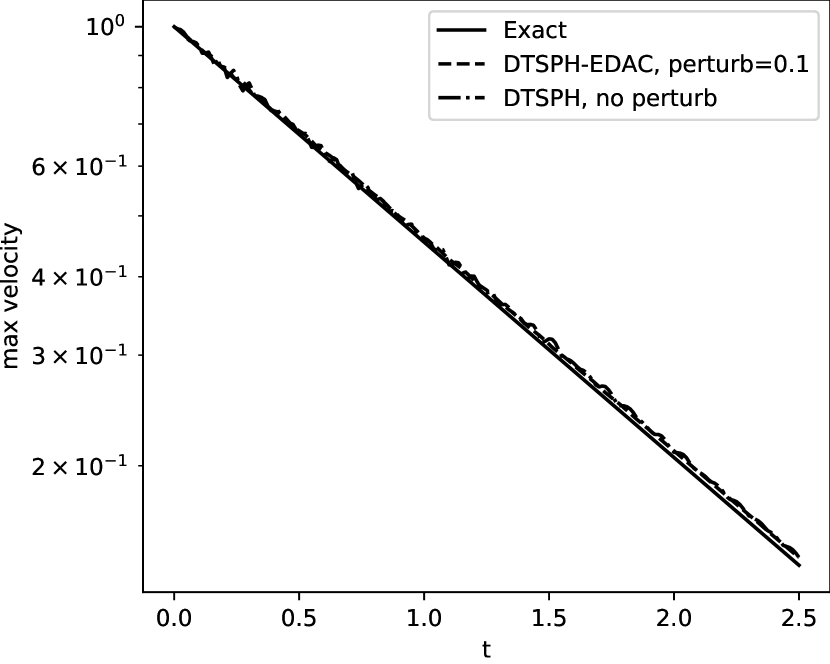
(a) Decay of maximum velocity with time.

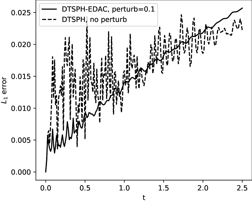
(b) $L_{1}$ error of velocity magnitude with time.

Figure 1: Comparison of perturbation (of atmost $\Delta x/10$) and without any perturbation.

Fig. 1(a) shows the decay of the velocity compared with the exact solution for the case where there is no initial perturbation and with a small amount of perturbation (of at most $\Delta x/10$). As can be clearly seen, the introduction of the perturbation significantly improves the results. This is clearly seen in the $L_{1}$ norm of the error in the velocity magnitude in Fig. 1(b). While we have not shown this, the results are similar for simulations made using most other schemes including the new scheme, TVF, and the EDAC. Given this, we henceforth use a small initial perturbation for the results for the Taylor-Green vortex problem.

4.1.2 Advection of particles in pseudo-time

As discussed earlier, it is important to study the effect of moving the particles in pseudo-time as against keeping them frozen in pseudo-time. If we find that there is no significant advantage gained by moving the particles in pseudo-time, we can simplify the implementation of the scheme as well as improve its performance considerably.

We consider the Taylor Green problem and compare the results of simulations where we advect the particles and where we hold them frozen. The rest of the parameters are held fixed. The same small perturbation is added to the initial particle position. Parameters used for this simulation are, initial particle spacing $\Delta x=\Delta y=0.01$, Reynolds number $Re=100$, the value of $\beta=5$, time step $\Delta t=0.00125$, and tolerance of $\epsilon=10^{-6}$.

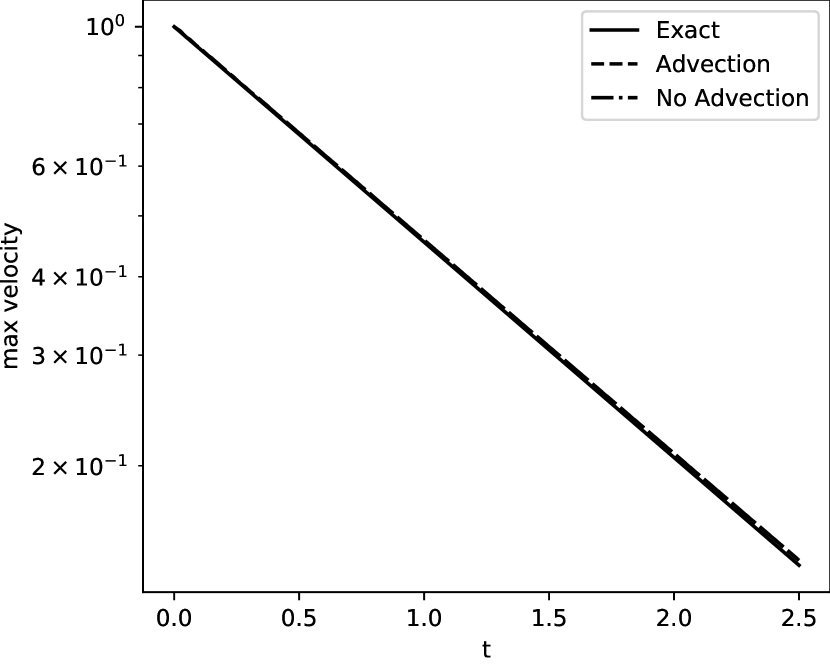
(a) Decay of maximum velocity with time.

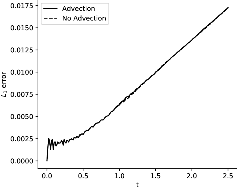
(b) $L_{1}$ error in the velocity magnitude with time.

Figure 2: Velocity decay plot for $Re=100$ for both advection and no advection of particles in pseudo time as compared with the exact solution for $Re=100$.

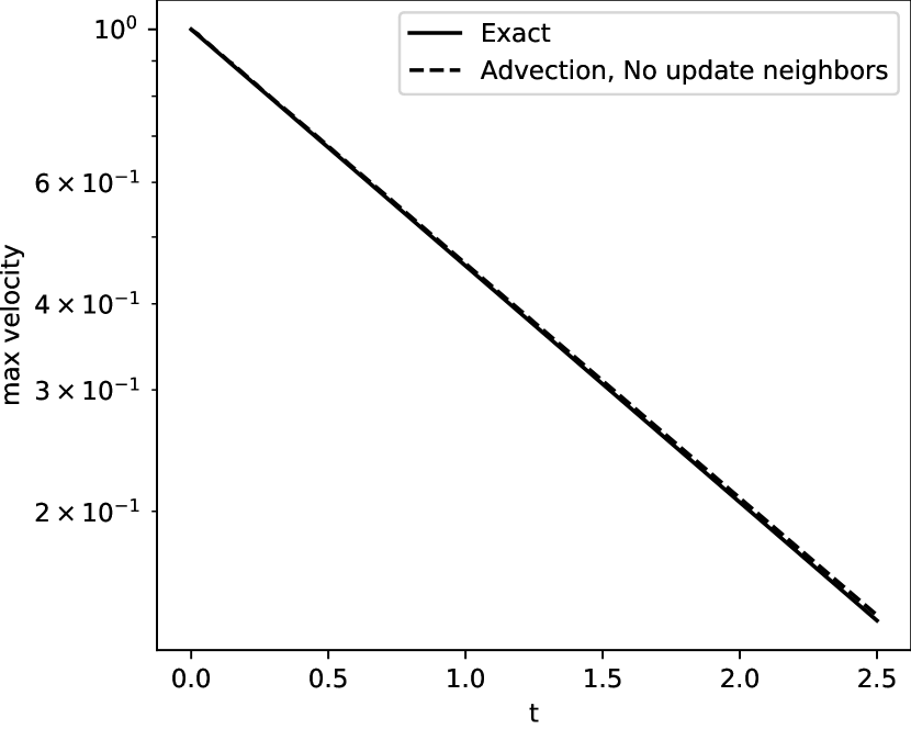
(a) Decay of maximum velocity with time.

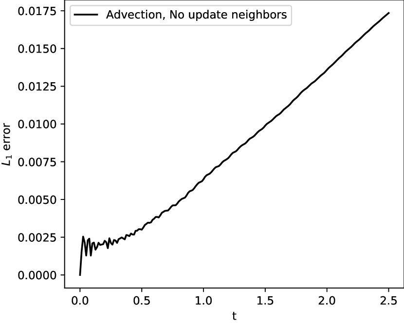
(b) $L_{1}$ error in the velocity magnitude with time.

Figure 3: Comparison for decay rates with time and $L_{1}$ errors in velocity for advection and without advection cases while no update in the neighbour particles.

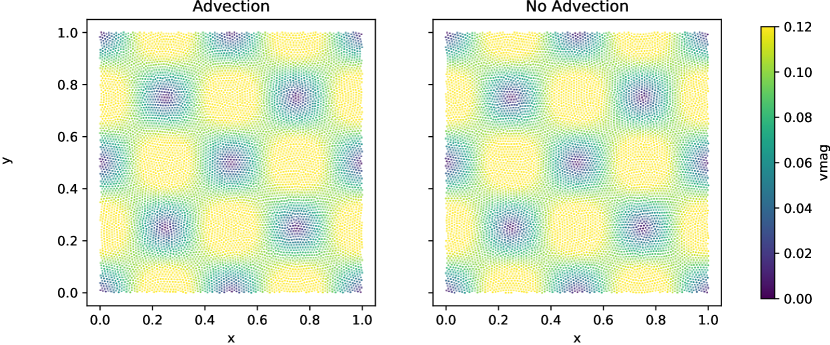
Figure 4: Particle plots for the Taylor-Green problem with advection and without advection in pseudo time while updating the neighbours. Plots are shown at $t=2.5s$ with $Re=100$.

We recall that when we advect the particles in pseudo-time, we need to update the neighbors, however the displacements are very small and this is not necessary. We perform simulations to see if the differences are significant. Fig. 2(a) shows the decay rate for the case with and without advection in pseudo-time while updating the neighbours. There are no noticeable differences in the results and the plots for each case lie on each other. This is also seen in Fig. 2(b) which shows the $L_{1}$ error. Fig. 3(a) and Fig. 3(b) show the decay rate and the $L_{1}$ error in the velocity magnitude while not updating the neighbours resulting in a similar conclusion that movement of particles in pseudo-time is too small to significantly influence the results.

Scheme	CPU time (secs)
DTSPH frozen	326.87
DTSPH advect, no update neighbors	638.62
DTSPH advect, update neighbors	1934.21

Table 1: CPU time taken for $2.5$ secs of Taylor-Green simulation with $100\times 100$ particles, with advection and without advection in pseudo time.

While the accuracy is unaffected, the performance is significantly different as can be seen from Table 1. This shows that advection of particles reduces performance by close to a factor of two. This increase in performance is largely due to the fact that we re-calculate the neighbour particles when we advect them. There is also some increase due to the additional computations required for the advection. Fig. 4 shows the particle plots with color representing velocity magnitude for the case where the particles are advected and frozen. The results look identical. Based on these results, we do not advect the particles in pseudo-time for any of the other simulations.

4.1.3 The influence of $\beta$

The parameter $\beta$ is the ratio of $c/V_{ref}$, as discussed earlier. The pseudo-timestep is also determined such that $\Delta t=\beta\Delta\tau$. In this section we consider the Taylor-Green problem simulated at $Re=100$ using $100\times 100$ particles, using the new scheme with different values of $\beta$ chosen between 2 and 20 for a tolerance $\epsilon=10^{-4}$, and run for a simulation time of $t=1$ sec.

Figs. 5(a) and 5(b) show the decay rate and the $L_{1}$ error in the velocity for the different cases. From these it appears that $\beta$ between 5 – 20 works well. We use a value of $\beta=10$ in all simulations unless explicitly mentioned.

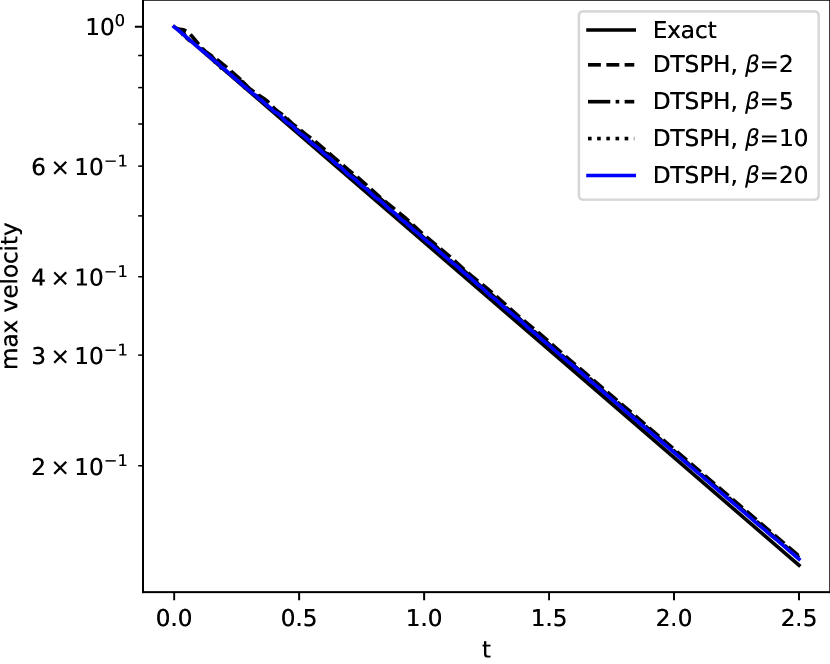
(a) Decay of maximum velocity with time.

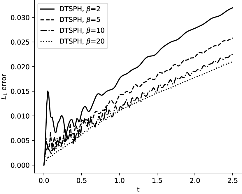
(b) $L_{1}$ error of velocity magnitude with time.

Figure 5: Decay rate of the maximum velocity and the $L_{1}$ error in the velocity magnitude for $\beta$ values of $[2,5,10,20]$ for the DTSPH scheme with an error tolerance of $10^{-4}$.

4.1.4 Changing the convergence tolerance parameter $\epsilon$

We next choose $\beta=10$ and vary the tolerance from $10^{-2}$ to $10^{-5}$. Fig. 6(a) shows the decay rates as the tolerance is changed and Fig. 6(b) shows the $L_{1}$ error in the velocity. These results clearly show that reducing the tolerance improves the accuracy. However, we do see that the solutions are by-and-large robust to changes in $\epsilon$ over a very large range. As expected, increase in the tolerance leads to increase in the simulation time taken as seen in Table. 2.

$\epsilon$	CPU time (secs)
0.01	120.22
0.0001	133.87
1e-05	305.88

Table 2: CPU time time taken for a simulation time of $2.5$ secs with $100\times 100$ particles with varying tolerance.

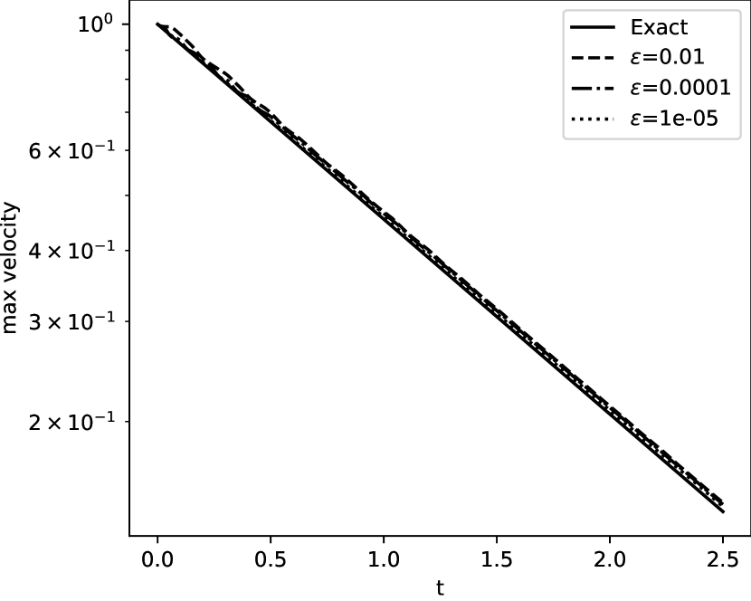
(a) Decay of maximum velocity with time.

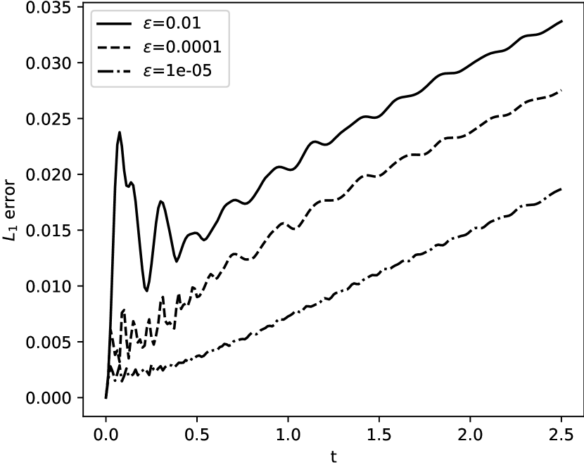
(b) $L_{1}$ error in the velocity magnitude with time.

Figure 6: Comparision for various tolerance $(\epsilon)$ ranging from $10^{-2}$ to $10^{-5}$.

4.1.5 Varying Reynolds number

We simulate the problem at $Re=1000$ using the most appropriate parameters based on the previous results. The DTSPH scheme is used with a quintic spline kernel, maximum initial random particle displacement of $\Delta x/10$, with a tolerance of $\epsilon=10^{-3}$, and $\beta=5$ for different initial particle arrangement of $25\times 25$ to $200\times 200$ and simulated for $2.5$ secs.

Fig. 7(a) shows the maximum velocity decay as well as the $L_{1}$ error of the velocity magnitude for the case of $Re=100$. Fig. 7(b) shows the same for $Re=1000$. It can be seen that in the case of $Re=1000$ that there is a clear reduction in the errors as the resolution is increased. In the case of $Re=100$, it appears that the errors are lower for the $50\times 50$ resolution and increase by a small amount as the resolution is increased. We believe that this occurs because of possible issues with the convergence of the discretization of the diffusive terms in the governing equations. We point out that at $Re=500$ we obtain similar convergence as in the case of $Re=1000$ showing that issue is not with the convergence of the DTSPH scheme per-se. These results show that the new scheme performs very well.

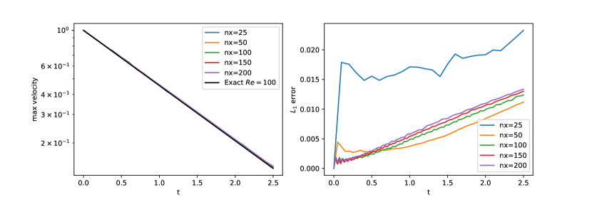
(a) Decay of maximum velocity with time and the $L_{1}$ error in the velocity magnitude for $Re=100$.

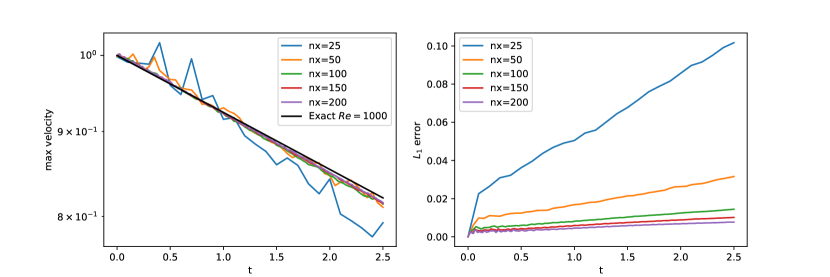
(b) Decay of maximum velocity with time and the $L_{1}$ error in the velocity magnitude for $Re=1000$.

Figure 7: Comparison of results for the Taylor-Green problem using five different particle configuration between $25\times 25$ to $200\times 200$. Shown are the results for the Reynolds number of $Re=100$ and $1000$.

4.1.6 Comparision with other schemes

Here we simulate the problem for $t=2.5s$ for $Re=100$ using the new DTSPH scheme comparing it with WCSPH, $\delta$-SPH, and EDAC. The quintic spline kernel is used for all the schemes with $h=\Delta x$. For all the cases the particles are perturbed by atmost $\Delta x/10$. For DTSPH, we use $\beta=10$ with a tolerance of $\epsilon=10^{-4}$. We use an initial configuration of $100\times 100$ particles.

As can be seen from the results shown in Fig. 8, the new scheme is more accurate than the standard WCSPH scheme. The scheme is more accurate than the standard $\delta$-SPH scheme. We note that we do not employ any form of shifting for the $\delta$-SPH and WCSPH scheme cases. The scheme is not more accurate than the EDAC scheme as in the EDAC scheme, the particles are also regularized using the transport velocity formulation which significantly improves the results. As can be seen from the Table 3, the new scheme is anywhere from 1.9 to 2.8 times faster than the other schemes.

In Fig. 9, we show the streamlines as well as the particle plot with the color indicating pressure at $t=2.5$secs for the DTSPH case for $Re=100$. As can be seen the particle distribution is smooth.

Scheme	CPU time (secs)
DTSPH	124.49
WCSPH	239.70
EDAC	275.43
$\delta$-SPH	347.98

Table 3: CPU time time taken for a simulation time of $2.5$ secs with $100\times 100$ particles for various schemes.

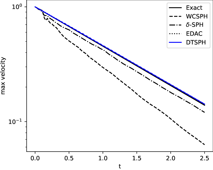
(a) Decay of maximum velocity with time.

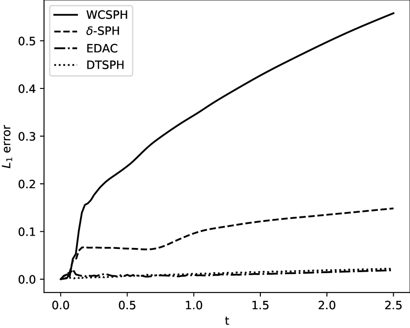
(b) $L_{1}$ error in the velocity magnitude with time.

Figure 8: Comparision of DTSPH with other schemes for the simulation of Taylor-Green problem, with $Re=100$ and using $100\times 100$ particles.

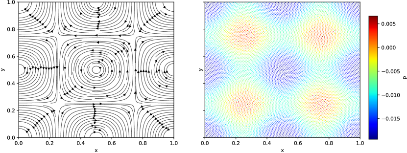
Figure 9: Particle plots for the Taylor-Green problem, with $100\times 100$ particles in the initial configuration, showing streamlines on the left and pressure on the left at $t=2.5s$.

4.2 The lid-driven-cavity problem

We next consider the classic lid-driven-cavity problem. This is a fairly challenging problem to simulate with SPH [9, 30, 31]. The fluid is placed in a unit square with a lid moving with a unit speed to the right. The bottom and side walls are treated as no-slip walls. The Reynolds number of the problem is given by $Re=\frac{V}{\nu}$, where $V$ is the lid velocity. We use a quintic spline kernel with $h=\Delta x$. The problem is simulated at $Re=100$ using a $50\times 50$, $100\times 100$, and $150\times 150$ grid for a simulation time of $t=10s$ until there is no change in the kinetic energy of the system. For the DTSPH scheme we use a $\beta=10$ with a tolerance $\epsilon=10^{-4}$. The results are compared with those of the TVF scheme[9] and the established results of Ghia et al. [32].

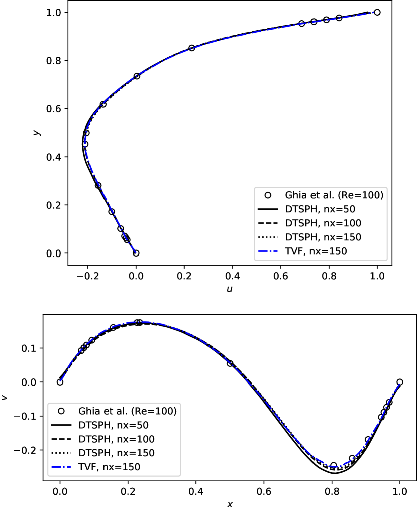
Figure 10: Velocity profiles $u$ vs. $y$ and $v$ vs. $x$ for the lid-driven-cavity problem at $Re=100$ with three initial particle arrangement of $50\times 50$, $100\times 100$, and $150\times 150$. Here we compare DTSPH with TVF and the results of [32].

Fig. 10, shows the centerline velocity profiles for $u$ vs. $y$ and $v$ vs. $x$ for different resolutions of particles. It is seen that the TVF scheme produces better results as expected. However, the results of the new scheme are in good agreement. In Fig. 11, we show the particle distribution with the velocity magnitude on the left and streamlines on the right.

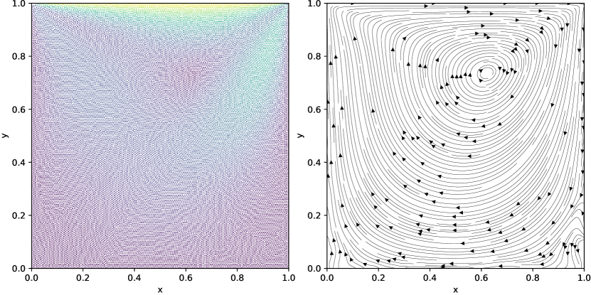
Figure 11: Particle plots for the cavity problem, with $150\times 150$ particles in the initial configuration, showing the velocity magnitude on the left and streamlines on the right at $t=10s$.

4.2.1 Steady Lid-driven cavity

In order to show that we are able to obtain steady state results, we employ the steady state equations discussed in Section 2.3 to solve the lid-driven-cavity problem. We solve the problem until there is no change in the kinetic energy of the system. We simulate the problem using a quintic spline kernel for $Re=100$ and $Re=1000$ using a $50\times 50$, $100\times 100$ and $150\times 150$ particle grid. For $Re=100$ we simulate the problem up to $\tau=10$ and for $Re=1000$ we simulate up to $\tau=50$.

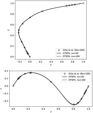
Figure 12: Velocity profiles for the lid-driven-cavity using the steady state simulation procedure for $Re=100$ with initial partial arragement of $50\times 50$, $100\times 100$, and $150\times 150$ compared with the results of [32].

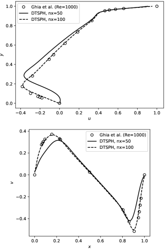
Figure 13: Velocity profiles for the lid-driven-cavity using the steady state simulation procedure for $Re=1000$ with initial partial arragement of $50\times 50$, $100\times 100$, and $150\times 150$ compared with the results of [32].

Fig. 12 shows the velocity profiles for the $Re=100$ case and Fig. 13 shows velocity profiles for the $Re=1000$ case.

These results show that we are able to simulate internal flows very well using the new DTSPH scheme. We have also demonstrated that the steady-state equations also work very well. We next consider problems that involve a free-surface.

4.3 Square patch

The square patch problem [33, 34, 35] is a free surface problem where a square patch of fluid of side $L$ is subjected to the following initial conditions,

$$u_{0}(x,y) =\omega y,$$ (47)

$$v_{0}(x,y) =-\omega x,$$

$$p_{0}(x,y)=\rho\sum_{m}^{\infty}\sum_{n}^{\infty}-\frac{32\omega^{2}/(mn\pi^{2})}{\left[{\left(\frac{n\pi}{L}\right)}^{2}+{\left(\frac{m\pi^{2}}{L}\right)}^{2}\right]}\sin\left(\frac{m\pi x^{*}}{L}\right)\sin\left(\frac{n\pi y^{*}}{L}\right)m,n\in\mathbb{N}_{odd},$$ (48)

where $X^{*}=x+L/2$ and $y^{*}=y+L/2$.

We simulate this problem for $t=3s$ using the DTSPH, and EDAC schemes for comparison. In this case, the EDAC simulations also employ particle shifting [29]. The quintic spline kernel with $h/\Delta x=1.3$ is used for all the schemes, artificial viscosity $\alpha=0.1$ is used for all the schemes. For the DTSPH scheme, $\beta=10$ with a tolerance $\epsilon=10^{-3}$ is used. Two different initial configurations of $50\times 50$ and $200\times 200$ particles are used.

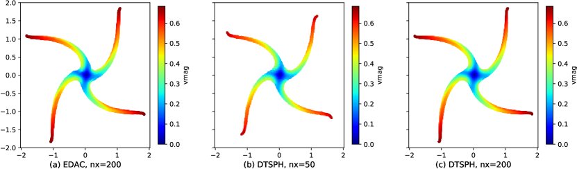
Figure 14: Particle distribuiton plots at $t=3$ secs for the square patch problem. Artificial viscosity is used in all the schemes. Top row corresponds to $50\times 50$ particles, and the bottom row corresponds to $100\times 100$ particles. In column (a) EDAC scheme is used, with $200\times 200$ particles, column (b) indicates DTSPH scheme with a tolerance of $\epsilon=10^{-3}$, and $50\times 50$ particles, and in column (c) DTSPH scheme is used with a tolerance of $\epsilon=10^{-3}$, and $200\times 200$ particles.

The particle distribution for each scheme at the end of $t=3s$ is shown in Fig. 14. The plots of DTSPH and EDAC are in good agreement with each other showing that the new scheme is as good as the EDAC scheme.

4.4 Elliptical drop

The elliptical drop problem was first solved in the context of the SPH by Monaghan [3]. This problem is also solved in the context of truly incompressible SPH [34, 36, 37]. In this problem an initially circular drop of inviscid fluid having unit radius is subjected to the initial velocity field given by $-100x\hat{i}+100y\hat{j}$. The outer surface is treated as a free surface. Due to the incompressibility constraint on the fluid there is an evolution equation for the semi-major axis of the ellipse.

This problem is simulated using the DTSPH, $\delta$-SPH (without shifting), and EDAC (with shifting) respectively. An artificial viscosity parameter of $\alpha=0.15$ is used for all the schemes. An error tolerance of $\epsilon=10^{-4}$ is used for the DTSPH and scheme. $\beta=10$, $\Delta x=0.02$, $h=1.3\Delta x$ and a quintic spline kernel is used for all the schemes. The simulation is run for $t=0.0076s$.

Fig. 15 shows the distribution of particles for different schemes. The colors indicate the pressure. As can be seen, the DTSPH and EDAC results are similar. It is important to note that all the pressure values are in a similar range with none of the schemes exhibiting severe noise in the pressure.

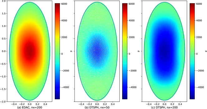
Figure 15: The distribution of particles for the elliptical drop problem at $t=0.0076$ seconds. The plot (a) is with the EDAC using $200\times 200$ particles. Plot (b) is that of the new DTSPH scheme with $50\times 50$ particles, (c) uses DTSPH with $200\times 200$. The solid blue line is the exact solution for the shape of the drop and the colors indicate the pressure.

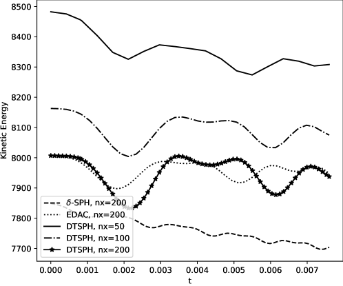
Figure 16: The kinetic energy with time of the Elliptical drop problem as computed with DTSPH, $\delta$-SPH, and EDAC schemes.

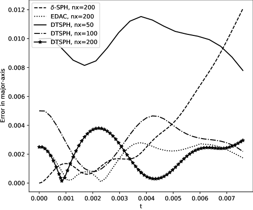
Figure 17: Error in computed size of semi-major axis of the elliptical drop problem compared with the exact solution for the DTSPH, $\delta$-SPH and EDAC schemes.

Fig. 16, shows the evolution of the kinetic energy, the results are similar for DTSPH and EDAC schemes. This is to be expected. However it is interesting to note that the kinetic energy of the $\delta$-SPH scheme decays faster than the other schemes. Fig. 17 shows the error in the semi-major axis as compared to the exact solution. The DTSPH and EDAC both perform slightly better than the $\delta$-SPH scheme. The results indicate that the new scheme performs well in comparison with state of the art weakly-compressible schemes.

4.5 Dam-break in 2 dimensions

A two dimensional dam-break over a dry bed [31, 11, 36] is considered next. The DTSPH and the standard EDAC schemes are compared. The simulation is performed for $1s$. The quintic spline kernel is used with $h/\Delta x=1.0$, and an artificial viscosity of $\alpha=0.1$ is used for all the schemes. A tolerance of $\epsilon=10^{-4}$ is used for DTSPH.

The problem considered is described in [38] with a block of fluid column of height $h=2m$, width $w=1m$. The block is released under gravity which is assumed to be $-9.81m/s^{2}$.

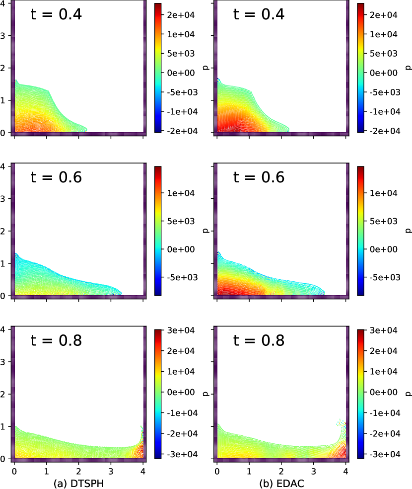
Figure 18: Particle distribution plots with color indicating pressure for the dam-break 2D problem at various times. DTSPH is shown on the left, and EDAC is shown on the right. Top row is at $t=0.4$ secs, second row is at $t=0.6$ secs, and bottom row is at $t=0.8$ secs.

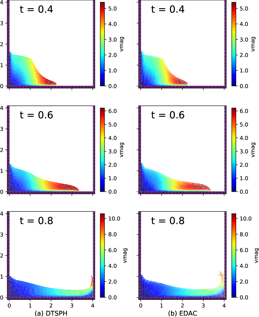
Figure 19: Particle distribution plots with color indicating velocity magnitude for the 2D dam-break problem at variuos times. DTSPH scheme is shown on the left, and EDAC is shown on the right. Top row is at $t=0.4$ secs, the second row is at $t=0.2$ secs, and bottom row is at $t=0.8$ secs.

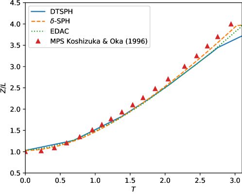
Figure 20: Position of the toe of the dam versus time of DTSPH, WCSPH, $\delta$-SPH and EDAC, as compared with the simulation of [39]. $Z$ is the distance of toe of the dam from the left wall and $L$ is the initial width of the dam

For the DTSPH and EDAC schemes, the particle distribution is shown in Fig. 18 at various times with color indicating pressure. Fig. 19 shows the particle distribution with color indicating velocity magnitude at various times. The results of the new scheme seem largely comparable with that of the EDAC scheme. The results also show the improvements obtained by the addition of diffusive term in the pressure evolution equation. This significantly reduces the noise. The standard EDAC results are very similar to those of the $\delta$-SPH and are hence not shown. Fig. 20 plots the position of the toe of the dam versus time as compared with the results of the Moving Point Semi-implicit scheme of [39]. The results of the DTSPH scheme are in good agreement with those of the EDAC scheme.

4.6 Dam-break in three dimensions

A three dimensional case is shown to demonstrate the performance of the new scheme as compared to the EDAC scheme. This is an important case as the previous problems only require a smaller number of particles. We consider a three-dimensional dam break over a dry bed with an obstacle. A cubic spline kernel is used for both the new scheme and the EDAC with $h/\Delta x=1.3$ and artificial viscosity $\alpha=0.1$. The problem is simulated for a total time of 1 second. We do not use any particle shifting in this case.

The problem considered is described in [38] with a block of fluid column of height $h=0.55m$, width $w=1.0m$ and length $l=1.228m$. The container is $3.22m$ long. The block is released under gravity with an acceleration of $-9.81m/s^{2}$. Both schemes are simulated with a fixed time step. For both schemes we use a CFL of 0.25. The speed of sound for the EDAC case is set to $10\sqrt{2gh}$, where $h$ is the height of the water column. For the DTSPH, we use a time step of $\frac{0.25h}{\sqrt{2gh}}$, and use $\beta=10,\epsilon=10^{-3}$. The particle spacing, $\Delta x=0.02$, leading to around 240000 particles in the simulation.

(a) EDAC scheme.

(b) DTSPH scheme.

Figure 21: Dam-break 3D particle distribution at various times, first row is at $t=0.4$ secs second row is at $t=0.6$ secs and third row is at $t=1.0$ secs. The left column is EDAC scheme and right column is the DTSPH scheme.

Fig. 21 shows the particle distribution at various times for both the schemes. This indicate that the new scheme produces good results. Table 4 shows the time taken for the different 3D dam break simulations. Depending on the tolerance chosen, we are able to obtain between a 1.7 to 7.16 fold improvement in performance as compared to the EDAC scheme. We note that as the tolerance $\epsilon$ is reduced, the DTSPH requires more iterations in pseudo-time in order to attain convergence and this reduces the performance. However even with lower tolerance values we are able to obtain very good results. In the next section we demonstrate the performance achievable with the new scheme for different problems.

Scheme	$\epsilon$	CPU time (secs)
DTSPH	0.001	563.19
DTSPH	0.0001	2404.97
EDAC	NA	4035.25

Table 4: CPU time time taken for different simulations of the 3D dam break problem.

4.7 Performance

The performance of DTSPH is compared with that of other schemes for various problems. In Table 5 we list the different problems and the speedup obtained by using the new scheme.

As we have seen before, for the dam-break problem in three dimensions it can be seen that DTSPH (with a tolerance of $10^{-3}$) can be up to 7.16 times faster than the standard EDAC scheme. When a very low tolerance is used, the scheme is about 1.7 times faster this is only to be expected as lower tolerances require many more iterations to obtain a converged pressure. For the two-dimensional dam break cases, the new scheme is about 3.5 times faster than the EDAC or the $\delta$-SPH. For the unsteady cavity problem at $Re=100$ with a $150\times 150$ grid of particles, we get up to a 7 times performance improvement. This is quite significant since in these cases we have compared these cases where the effective Mach number is 0.1. Given this, the primary advantage with the DTSPH is that it can take a time step that is 10 times smaller. Hence in this case a speed-up of close to 7 suggests that it is an efficient scheme.

Problem	Scheme	Speed up
Dam break 3D	EDAC vs. DTSPH ($\epsilon=10^{-3}$)	7.16
Dam break 3D	EDAC vs. DTSPH ($\epsilon=10^{-4}$)	1.68
Dam break 2D	EDAC vs. DTSPH	3.57
Dam break 2D	EDAC vs. $\delta$-SPH	3.66
Cavity	TVF vs DTSPH	6.87

Table 5: Speed-up obtained for different simulations when using the DTSPH scheme.

The suite of benchmarks considered shows that the new scheme is robust, simulates a variety of problems, and is as accurate as the EDAC scheme. In addition it is very efficient and can be as much as seven times faster than the EDAC scheme. Indeed, it is possible to improve the performance even more by caching the values of the kernel and kernel gradients during the pseudo-time iterations but we have not done this in the present work.

5 Conclusions

In this paper we propose a scheme called Dual-Time stepped SPH (DTSPH) that employs a dual-time stepping approach for incompressible fluid flow simulations. The method has been demonstrated with the EDAC formulation [12]. There are a few recent developments in the literature that employ a similar approach [17, 19] but these implementations are not efficient despite the ability to use much smaller timesteps than the WCSPH scheme. We find that by not moving the particles in pseudo-time we are able to improve performance significantly without loss of accuracy as attested by our simulations. We show that the scheme is robust and accurate. Through several benchmarks in two and three dimensions we show that the scheme produces results that are as accurate as the $\delta$-SPH scheme [10] as well as the EDAC scheme [12] while being up to seven times faster. The method is matrix-free and may be implemented in the context of any explicit SPH scheme. The DTSPH method does introduce a few new parameters in the form of the term $\beta=\Delta t/\Delta\tau$ and the tolerance $\epsilon$. We discuss how these parameters can be set based on rational considerations. For a reasonable choice of parameters, the performance of the method is comparable to that of incompressible SPH schemes. An open source implementation of the new scheme is provided and the manuscript is fully reproducible. Given the results presented with this method, a promising line of future work would be to apply this to the case of solid mechanics problems where the timesteps are very small. A method of this kind would provide significant computational advantages. This would also be of considerable importance in the area of fluid-structure-interaction which is an important emerging area of investigation with the SPH method.

References

Appendix

This section provides a derivation of the perturbation velocity that is given in equation (17).

Using trapezoidal rule for integration, the displacement of the particle in pseudo time from the initial state $(\mathbf{r}^{k=0},\mathbf{V}^{k=0},0)$ to the current pseudo time state $(\mathbf{r}^{k},\mathbf{V}^{k+1},\Delta t)$ when $k\rightarrow\infty$ is given by,

$$\mathbf{r}^{k+1}-\mathbf{r}^{n}=\Delta t\frac{(\mathbf{V}^{k+1}+\mathbf{V}^{n})}{2},$$ (49)

similarly, using the trapezoidal rule of integration for the displacement between states in pseudo time is given by,

$$\mathbf{r}^{k+1}=\mathbf{r}^{k}+\frac{\Delta\tau}{2}(\mathbf{\tilde{V}}^{k}+\mathbf{\tilde{V}}^{k+1}).$$ (50)

Expanding $\mathbf{r}^{k}$ in terms of $\mathbf{r}^{0}$ (i.e. $k=0$)is,

$$\mathbf{r}^{k+1}=\mathbf{r}^{0}+\frac{\Delta\tau}{2}\mathbf{\tilde{V}}^{0}+\Delta\tau\sum_{j=1}^{k}\mathbf{\tilde{V}}^{j}+\frac{\Delta\tau}{2}\mathbf{\tilde{V}}^{k+1},$$ (51)

where, the position before pseudo time iteration $\mathbf{r}^{0}$ is given by (11).

Substitute the above equation (51) into the equation (49) we get,

$$\mathbf{r}^{0}-\mathbf{r}^{n}+\frac{\Delta\tau}{2}(\mathbf{\tilde{V}}^{0}+\mathbf{\tilde{V}}^{k+1})+\Delta\tau\sum_{j=1}^{k}\mathbf{\tilde{V}}^{j}=\Delta t\frac{(\mathbf{V}^{k+1}+\mathbf{V}^{n})}{2}.$$ (52)

Rearranging terms to get $\mathbf{V}^{k+1}$ as,

$$\mathbf{V}^{k+1}=\frac{2}{\Delta t}\left(\mathbf{r}^{0}-\mathbf{r}^{n}\right)+\frac{\Delta\tau}{\Delta t}(\mathbf{\tilde{V}}^{0}+\mathbf{\tilde{V}}^{k+1})+\frac{2\Delta\tau}{\Delta t}\sum_{j=1}^{k}\mathbf{\tilde{V}}^{j}-\mathbf{V}^{n}.$$ (53)

Similarly $\mathbf{V}^{k}$ is written as,

$$\mathbf{V}^{k}=\frac{2}{\Delta t}\left(\mathbf{r}^{0}-\mathbf{r}^{n}\right)+\frac{\Delta\tau}{\Delta t}(\mathbf{\tilde{V}}^{0}+\mathbf{\tilde{V}}^{k})+\frac{2\Delta\tau}{\Delta t}\sum_{j=1}^{k-1}\mathbf{\tilde{V}}^{j}-\mathbf{V}^{n}.$$ (54)

Subtract (54) from (53),

$$\mathbf{V}^{k+1}-\mathbf{V}^{k}=\frac{\Delta\tau}{\Delta t}(\mathbf{\tilde{V}}^{k+1}+\mathbf{\tilde{V}}^{k}).$$ (55)

By substituting eq. (14) we get,

$$\mathbf{\tilde{V}}^{k}=\frac{\Delta t}{\Delta\tau}(\mathbf{V}^{k+1}-\mathbf{V}^{k})=\Delta t{\left(\frac{d\mathbf{V}}{d\tau}\right)}^{k+1/2}.$$ (56)

Note that in the limit $k\rightarrow\infty$, $\mathbf{\tilde{V}}^{k+1}$ goes to zero, and $\lim_{k\rightarrow\infty}\mathbf{V}^{k+1}=\mathbf{V}^{n+1}$.

References

- Gingold and Monaghan [1977] Gingold, R.A., Monaghan, J.J.. Smoothed particle hydrodynamics: Theory and application to non-spherical stars. Monthly Notices of the Royal Astronomical Society 1977;181:375–389.
- Lucy [1977] Lucy, L.B.. A numerical approach to testing the fission hypothesis. The Astronomical Journal 1977;82(12):1013–1024.
- Monaghan [1994] Monaghan, J.J.. Simulating free surface flows with SPH. Journal of Computational Physics 1994;110:399–406.
- Cummins and Rudman [1999] Cummins, S.J., Rudman, M.. An SPH projection method. Journal of Computational Physics 1999;152:584–607.
- Shao and Lo [2003] Shao, S., Lo, E.Y.. Incompressible SPH method for simulating newtonian and non-newtonian flows with a free surface. Advances in Water Resources 2003;26(7):787 – 800. doi:10.1016/S0309-1708(03)00030-7.
- Gray et al. [2001] Gray, J., Monaghan, J., Swift, R.. Sph elastic dynamics. Computer Methods in Applied Mechanics and Engineering 2001;190(49):6641–6662. doi:10.1016/S0045-7825(01)00254-7.
- Rafiee and Thiagarajan [2009] Rafiee, A., Thiagarajan, K.P.. An SPH projection method for simulating fluid-hypoelastic structure interaction. Computer Methods in Applied Mechanics and Engineering 2009;198(33):2785–2795. doi:10.1016/j.cma.2009.04.001.
- Khayyer et al. [2018] Khayyer, A., Gotoh, H., Falahaty, H., Shimizu, Y.. An enhanced ISPH–SPH coupled method for simulation of incompressible fluid–elastic structure interactions. Computer Physics Communications 2018;232:139–164. doi:10.1016/j.cpc.2018.05.012.
- Adami et al. [2013] Adami, S., Hu, X., Adams, N.. A transport-velocity formulation for smoothed particle hydrodynamics. Journal of Computational Physics 2013;241:292–307. doi:10.1016/j.jcp.2013.01.043.
- Antuono et al. [2010] Antuono, M., Colagrossi, A., Marrone, S., Molteni, D.. Free-surface flows solved by means of SPH schemes with numerical diffusive terms. Computer Physics Communications 2010;181(3):532 – 549. doi:10.1016/j.cpc.2009.11.002.
- Marrone et al. [2011] Marrone, S., Antuono, M., Colagrossi, A., Colicchio, G., Le Touzé, D., Graziani, G.. -SPH model for simulating violent impact flows. Computer Methods in Applied Mechanics and Engineering 2011;200:1526–1542. doi:10.1016/j.cma.2010.12.016.
- Ramachandran and Puri [2019] Ramachandran, P., Puri, K.. Entropically damped artificial compressibility for SPH. Computers and Fluids 2019;179(30):579–594. doi:10.1016/j.compfluid.2018.11.023.
- Hu and Adams [2007] Hu, X., Adams, N.. An incompressible multi-phase SPH method. Journal of Computational Physics 2007;227(1):264–278. doi:10.1016/j.jcp.2007.07.013.
- Solenthaler and Pajarola [2009] Solenthaler, B., Pajarola, R.. Predictive-corrective incompressible SPH. ACM Transactions on Graphics 2009;28(3):40:1–40:6. doi:10.1145/1531326.1531346.
- Ihmsen et al. [2014] Ihmsen, M., Cornelis, J., Solenthaler, B., Horvath, C., Teschner, M.. Implicit incompressible SPH. IEEE Trans Vis Comput Graph 2014;20(3):426–435. doi:10.1109/TVCG.2013.105.
- Muta et al. [2020] Muta, A., Ramachandran, P., Negi, P.. An efficient, open source, iterative isph scheme. Computer Physics Communications 2020;255:107283. doi:10.1016/j.cpc.2020.107283.
- Rouzbahani and Hejranfar [2017] Rouzbahani, F., Hejranfar, K.. A truly incompressible smoothed particle hydrodynamics based on artificial compressibility method. Computer Physics Communications 2017;210:10 – 28. doi:10.1016/j.cpc.2016.09.008.
- Chorin [1967] Chorin, A.J.. A numerical method for solving incompressible viscous flow problems. Journal of Computational Physics 1967;2(1):12 – 26. doi:10.1016/0021-9991(67)90037-X.
- Fatehi et al. [2019] Fatehi, R., Rahmat, A., Tofighi, N., Yildiz, M., Shadloo, M.S.. Density-based smoothed particle hydrodynamics methods for incompressible flows. Computers & Fluids 2019;185:22–33. doi:10.1016/j.compfluid.2019.02.018.
- Zhang et al. [2020] Zhang, C., Rezavand, M., Hu, X.. Dual-criteria time stepping for weakly compressible smoothed particle hydrodynamics. Journal of Computational Physics 2020;404:109135. doi:10.1016/j.jcp.2019.109135.
- Ramachandran et al. [2020] Ramachandran, P., Bhosale, A., Puri, K., Negi, P., Muta, A., Adepu, D., Menon, D., Govind, R., Sanka, S., Sebastian, A.S., Sen, A., Kaushik, R., Kumar, A., Kurapati, V., Patil, M., Tavker, D., Pandey, P., Kaushik, C., Dutt, A., Agarwal, A.. PySPH: a Python-based framework for smoothed particle hydrodynamics. arXiv preprint arXiv:190904504 2020;URL: https://arxiv.org/abs/1909.04504.
- Ramachandran [2016] Ramachandran, P.. PySPH: a reproducible and high-performance framework for smoothed particle hydrodynamics. In: Benthall, S., Rostrup, S., eds. Proceedings of the 15th Python in Science Conference. 2016:127 – 135. doi:10.25080/Majora-629e541a-011.
- Ramachandran [2018] Ramachandran, P.. automan: A python-based automation framework for numerical computing. Computing in Science & Engineering 2018;20(5):81–97. doi:10.1109/MCSE.2018.05329818.
- Monaghan [2005] Monaghan, J.J.. Smoothed Particle Hydrodynamics. Reports on Progress in Physics 2005;68:1703–1759.
- Morris et al. [1997] Morris, J.P., Fox, P.J., Zhu, Y.. Modeling low reynolds number incompressible flows using SPH. Journal of Computational Physics 1997;136(1):214–226. doi:10.1006/jcph.1997.5776.
- Ferrari et al. [2009] Ferrari, A., Dumbser, M., Toro, E.F., Armanini, A.. A new 3D parallel SPH scheme for free surface flows. Computers & Fluids 2009;38(6):1203–1217. doi:10.1016/j.compfluid.2008.11.012.
- Adami et al. [2012] Adami, S., Hu, X., Adams, N.. A generalized wall boundary condition for smoothed particle hydrodynamics. Journal of Computational Physics 2012;231(21):7057–7075. doi:10.1016/j.jcp.2012.05.005.
- Hughes and Graham [2010] Hughes, J., Graham, D.. Comparison of incompressible and weakly-compressible SPH models for free-surface water flows. Journal of Hydraulic Research 2010;48:105–117.
- Lind et al. [2012] Lind, S., Xu, R., Stansby, P., Rogers, B.. Incompressible smoothed particle hydrodynamics for free-surface flows: A generalised diffusion-based algorithm for stability and validations for impulsive flows and propagating waves. Journal of Computational Physics 2012;231(4):1499 – 1523. doi:10.1016/j.jcp.2011.10.027.
- Ghasemi V. et al. [2013] Ghasemi V., A., Firoozabadi, B., Mahdinia, M.. 2D numerical simulation of density currents using the SPH projection method. European Journal of Mechanics - B/Fluids 2013;38:38–46. doi:10.1016/j.euromechflu.2012.10.004.
- Lee et al. [2008] Lee, E.S., Moulinec, C., Xu, R., Violeau, D., Laurence, D., Stansby, P.. Comparisons of weakly compressible and truly incompressible algorithms for the SPH mesh free particle method. Journal of Computational Physics 2008;227(18):8417–8436. doi:10.1016/j.jcp.2008.06.005.
- Ghia et al. [1982] Ghia, U., Ghia, K.N., Shin, C.T.. High-Re solutions for incompressible flow using the Navier-Stokes equations and a multigrid method. Journal of Computational Physics 1982;48:387–411.
- Colagrossi [2005] Colagrossi, A.. A meshless lagrangian method for free-surface and interface flows with fragmentation. These, Universita di Roma 2005;URL: http://hdl.handle.net/10805/688.
- Khayyer and Gotoh [2013] Khayyer, A., Gotoh, H.. Enhancement of performance and stability of MPS mesh-free particle method for multiphase flows characterized by high density ratios. Journal of Computational Physics 2013;242:211–233. doi:10.1016/j.jcp.2013.02.002.
- Sun et al. [2017] Sun, P., Colagrossi, A., Marrone, S., Zhang, A.. The -SPH model: Simple procedures for a further improvement of the SPH scheme. Computer Methods in Applied Mechanics and Engineering 2017;315:25–49. doi:10.1016/j.cma.2016.10.028.
- Lind et al. [2016] Lind, S., Stansby, P., Rogers, B.. Incompressible–compressible flows with a transient discontinuous interface using smoothed particle hydrodynamics (SPH). Journal of Computational Physics 2016;309:129–147. doi:10.1016/j.jcp.2015.12.005.
- Rezavand et al. [2018] Rezavand, M., Taeibi-Rahni, M., Rauch, W.. An ISPH scheme for numerical simulation of multiphase flows with complex interfaces and high density ratios. Computers & Mathematics with Applications 2018;75(8):2658–2677. doi:10.1016/j.camwa.2017.12.034.
- Lee et al. [2010] Lee, E.S., Violeau, D., Issa, R., Ploix, S.. Application of weakly compressible and truly incompressible SPH to 3-d water collapse in waterworks. Journal of Hydraulic Research 2010;48:50–60. doi:10.1080/00221686.2010.9641245.
- Koshizuka and Oka [1996] Koshizuka, S., Oka, Y.. Moving-particle semi-implicit method for fragmentation of incompressible fluid. Nuclear Science and Engineering 1996;123:421–434.