Enhancement of Local Pairing Correlations in Periodically Driven Mott Insulators

Abstract

We investigate a model for a Mott insulator in presence of a time-periodic modulated interaction and a coupling to a thermal reservoir. The combination of drive and dissipation leads to non-equilibrium steady states with a large number of doublon excitations, well above the maximum thermal-equilibrium value. We interpret this effect as an enhancement of local pairing correlations, providing analytical arguments based on a Floquet Hamiltonian. Remarkably, this Hamiltonian shows a tendency to develop long-range staggered superconducting correlations. This suggests the possibility of realizing the elusive eta-pairing phase in driven-dissipative Mott Insulators.

The Floquet engineering of complex quantum systems is a very active line of research in today’s condensed matter physics Oka and Kitamura (2018). It consists in the design of periodic perturbations to achieve non-equilibrium driven states remarkably different from their undriven counterparts. Examples are the dynamical control of band topology Oka and Aoki (2009); Jotzu et al. (2014) and of magnetic interactions Görg et al. (2018) in ultracold atoms in optical lattices, and of effective Hamiltonian parameters in solids under intense laser-pulse excitation Kawakami et al. (2009); Singla et al. (2015); Subedi et al. (2014).

A useful description of a periodically driven quantum system is in terms of effective static Hamiltonians derived with large-frequency expansions Goldman and Dalibard (2014); Bukov et al. (2015a); Tsuji et al. (2011); Kitamura and Aoki (2016). In general, however, the drive affects also the distribution function of the system, eventually leading to thermalization to a trivial infinite-temperature state Lazarides et al. (2014); D’Alessio and Rigol (2014). Nevertheless, when heating can be avoided for finite but long times, interesting prethermal Floquet states can be observed. This is the case, for example, for very large drive frequency Abanin et al. (2015); Mori et al. (2016); Kuwahara et al. (2016); Abanin et al. (2017) or systems close to integrability Bukov et al. (2015b); Canovi et al. (2016); Weidinger and Knap (2016); Seetharam et al. (2018); Herrmann et al. (2018); Baum et al. (2018). In particular, Ref. Peronaci et al. (2018) showed that strong electronic correlations lead to finite-frequency prethermal states with remarkable properties as a function of drive frequency.

A natural question concerning the Floquet prethermal state is whether the coupling to external reservoirs would cancel out its interesting features, or rather preserve them and possibly make them more accessible. Particularly interesting is the possibility to control the distribution function of the system by means of a dissipation mechanism of the energy injected by the drive Iadecola et al. (2013, 2015); Seetharam et al. (2015, 2019); Hart et al. (2019).

To investigate this point, in this work we consider the Fermi-Hubbard model with a periodically driven interaction and coupled to a thermal reservoir. Starting from the Mott-insulating phase, our numerical calculations show that the combination of drive and dissipation leads to steady states that are not accessible in the corresponding isolated model. In particular, we reveal a regime with a remarkably large number of high-energy doublon excitations, well above the maximum equilibrium value for the half-filled repulsive Hubbard model.

We interpret this steady-state large double occupancy as an enhancement of local pairing correlations, and we describe the effect as a thermalization to a lowest-order Floquet Hamiltonian. Remarkably, we find that higher-order terms promote finite-momentum doublon superfluidity, namely staggered long-range pairing correlations among fermions ($\eta$-pairing), which spontaneously break the hidden SU${}_{\text{C}}(2)$ charge symmetry of the half-filled Hubbard model Yang (1989); Zhang (1990); Mitra et al. (2018). This suggests a nonequilibrium protocol for Floquet engineering exotic superconducting states in driven-dissipative Mott insulators, as also very recently investigated in similar contexts Kaneko et al. (2019); Tindall et al. (2019); Werner et al. (2019a); Li et al. (2019).

Our results are relevant for current experiments on laser-pumped organic Mott insulators Kawakami et al. (2009); Singla et al. (2015) and ultracold Fermi gases in driven optical lattices Messer et al. (2018); Sandholzer et al. (2019). We discuss the latter in particular, suggesting to explore a possibly overlooked regime in future experiments.

Model – The Hamiltonian of the driven-dissipative Fermi-Hubbard model reads $H=H_{\text{Hub}}+H_{\text{diss}}$, where:

$$H_{\text{Hub}}=\sum_{ij,\sigma}V_{ij}c^{\dagger}_{i\sigma}c_{j\sigma}+U(t)\sum_{i}(n_{i\uparrow}-\tfrac{1}{2})(n_{i\downarrow}-\tfrac{1}{2}),$$ (1)

$$H_{\text{diss}}=\sum_{i\alpha}\omega_{\alpha}b^{\dagger}_{i\alpha}b_{i\alpha}+\lambda\sum_{i\alpha}g_{\alpha}(n_{i}-1)(b_{i\alpha}+b_{i\alpha}^{\dagger}).$$ (2)

Here the $c$’s operators describe fermions hopping with amplitude $V_{ij}$ and subject to a driven local interaction $U(t\geq 0)=U_{0}+\delta U\sin\Omega t$. The bare density of states is semicircular with bandwidth $4V$ and we measure energy, frequency and inverse of time ($\hbar=1$) in units of $V$ Note (2). The thermal bath is implemented by independent sets of bosonic modes $b$’s which couple to density at each lattice site, with spectral function $J(\omega)=\sum_{\alpha}g^{2}_{\alpha}\delta(\omega-\omega_{\alpha})\propto\omega^{2}e^{-\frac{\omega}{\omega_{c}}}$ ($\omega_{c}=1$) and coupling $\lambda$ Note (2). Importantly, the bath allows energy dissipation but commutes with density $n_{i}=n_{i\uparrow}+n_{i\downarrow}$ and preserves particle-hole symmetry. The system remains half filled at all times ($\braket{n_{i\sigma}}=0.5$).

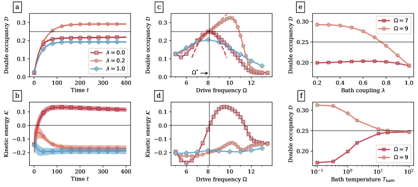
Figure 1: (a-b): Time evolution of double occupancy and kinetic energy for drive frequency $\Omega=9>\Omega^{*}$: oscillations (shaded area) and their average (symbols). Legend in (a) is common to (a-b-c-d). (c-d): Long-time averages as a function of drive frequency, and approximate analytical expressions based on Eq. (3) (dashed lines). (e-f): Long-time average of double occupancy as a function of bath coupling and of bath temperature for $\lambda=0.2$ and drive frequencies $\Omega=7<\Omega^{*}$ and $\Omega=9>\Omega^{*}$.

Starting from a thermal-equilibrium state, we calculate the time evolution by means of nonequilibrium dynamical mean-field theory (DMFT) Georges et al. (1996); Aoki et al. (2014) with the non-crossing approximation as impurity solver Eckstein and Werner (2010); Rüegg et al. (2013), including the effect of dissipation at weak coupling in $\lambda$ Chen et al. (2016) (see Supplemental Material Note (1) Sec. I for implementation details, and Sec. II for one-crossing-approximation benchmarks). We calculate double occupancy $\mathcal{D}(t)=\braket{n_{i\uparrow}(t)n_{i\downarrow}(t)}$, kinetic energy $\mathcal{K}(t)=\sum V_{ij}\braket{c^{\dagger}_{i\sigma}(t)c_{j\sigma}(t)}$, and local Green’s function $G_{\sigma}(t,t^{\prime})=-i\braket{\text{T}c_{i\sigma}(t)c^{\dagger}_{i\sigma}(t^{\prime})}$. For definiteness, we choose $U_{0}=8$ for the initial Mott-insulating state in equilibrium at $T=1$ Note (3) and $\delta U=2$ for the drive amplitude (see Supplemental Material Note (1) Sec. VI for a discussion on $\delta U$). The bath temperature is $T_{\text{bath}}=1$ unless specified differently. In absence of dissipation, Floquet prethermalization is observed at all frequencies except for the resonance $\Omega^{*}=8.12\simeq U_{0}$ Peronaci et al. (2018). We restrict ourselves to paramagnetic states, leaving the interplay of drive, dissipation and magnetism to future studies.

Time evolution – In the driven-dissipative model, as well as in the isolated case, double occupancy and kinetic energy display a separation of time scales between fast oscillations synchronized with the drive and a slowly varying average value. However, after a common transient, the thermal reservoir starts to be effective and changes substantially the long time behavior of both observables.

For weak bath coupling and drive above resonance, the double occupancy grows substantially larger than in the isolated model, going to a stationary average above $0.25$ (Fig. 1a, $\lambda=0.2$). Such a large value would be possible, at equilibrium, only if the interaction were attractive. This striking effect highlights the peculiarity of this non-equilibrium steady state, as we discuss thoroughly below.

Upon increasing the bath coupling (Fig. 1a, $\lambda=1.0$), the double occupancy decreases and eventually remains below the limit of $0.25$ at all times. Moreover, we notice that the bath is effective only after a transient time $\sim 1/\lambda^{2}$, which makes the regime of very weak coupling not accessible by the numerical simulation (see also Ref. Eckstein and Werner (2013)).

At the same time, the kinetic energy is also largely affected by dissipation (Fig. 1b). Here the effect is more intuitive: in the isolated model the drive leads to a prethermal state with positive kinetic energy, indicative of a population inversion Herrmann et al. (2018); Peronaci et al. (2018). On the other hand, the thermal reservoir dissipates the excess kinetic energy, which remains negative as at equilibrium, and inhibits the population inversion, as we also explicitly show below.

Long-time average – To study the role of drive frequency and bath coupling in a more systematic way, we consider the long-time average of double occupancy and kinetic energy. For weak bath coupling, the dissipative model has double occupancy larger than the isolated one at all frequencies (Fig. 1c, $\lambda=0.2$). However, a remarkable change happens crossing the resonance $\Omega^{*}\simeq U_{0}$. Below resonance, the dissipation has only a quantitative, rather weak effect. In contrast, above resonance, we systematically observe a large increase of double occupancy across the limit of $0.25$, as discussed previously for a selected frequency. Lower values are then recovered upon increasing the frequency further, as the system eventually becomes transparent to the drive.

Independent of the bath coupling, the kinetic energy of the dissipative model is rather featureless and negative for all frequencies (Fig. 1d, $\lambda=0.2,1.0$). Thus, the thermal reservoir cancels the region of positive kinetic energy characteristic of the isolated case (Fig. 1d, $\lambda=0.0$).

The difference between below and above resonance appears also in the dependence on bath coupling (Fig. 1e) and bath temperature (Fig. 1f). Below resonance ($\Omega=7$) the double occupancy is almost independent of bath coupling and decreases on lowering the bath temperature. Quite differently, above resonance ($\Omega=9$) it increases on lowering the bath temperature at weak bath coupling.

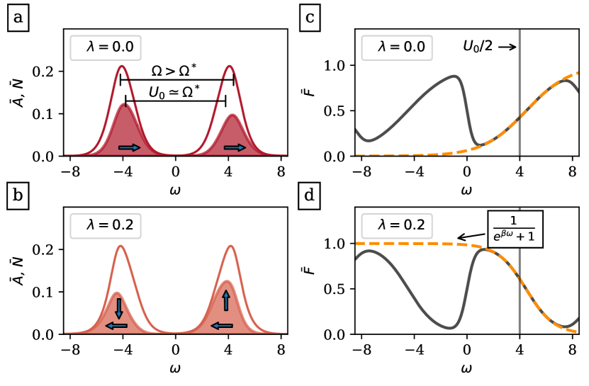
Figure 2: (a-b): Long-time average spectral function $\bar{A}(\omega)$ (solid line) and occupation function $\bar{N}(\omega)$ (filled area) of the isolated model ($\lambda=0$) and the dissipative model ($\lambda=0.2$) for drive frequency $\Omega=9>\Omega^{*}$. The isolated model (a) has population inversion, signaled by the blueshift of $\bar{N}(\omega)$ with respect to $\bar{A}(\omega)$ (arrows). In the dissipative model (b), the thermal reservoir cancels the population inversion (horizontal arrows) and unveils a non-thermal state with large double occupancy, signaled by the increase of $\bar{N}(\omega)$ in the high-energy band (vertical arrows). (c-d): Long-time average distribution function $\bar{F}(\omega)$ for the same parameters of (a-b) with Fermi-function fit around the Hubbard-band center. The extracted effective temperature is $T_{\text{eff}}=-1.6$ for the isolated model (c) and $T_{\text{eff}}=1.1\simeq T_{\text{bath}}$ for the dissipative one (d). See Supplemental Material Note (1) Fig. S3 for a plot of $T_{\text{eff}}(\Omega)$.

Notice that the observed behavior does not depend on the details of the bath spectral function as long as we deal with bosonic modes Note (2). In contrast, a fermionic reservoir does not lead to the same steady-state large double occupancy (see Supplemental Material Note (1) Sec. III) because it can change the local density even at zero hopping, spoiling the quasi-conservation of doublons which is the basis of Floquet prethermalization in this system Peronaci et al. (2018).

Spectral function – To gain insight into the nature of the steady state, we calculate the spectral function $\bar{A}(\omega)$ and occupation function $\bar{N}(\omega)$ as the average Wigner transforms of the retarded and lesser components of the local Green’s function Peronaci et al. (2018). While the spectral function is the same in the isolated and dissipative models, the occupation function, and thus the distribution function $\bar{F}(\omega)=\bar{N}(\omega)/\bar{A}(\omega)$, changes drastically for drive frequency above resonance and weak bath coupling.

In the isolated model, $\bar{N}(\omega)$ is shifted towards high energy with respect to $\bar{A}(\omega)$ (Fig. 2a). There is therefore a population inversion within the Hubbard bands. Indeed, the local behavior of $\bar{F}(\omega)$ for $\omega\simeq\pm U_{0}/2$ has the shape of a Fermi function with negative temperature (Fig. 2c).

The thermal reservoir completely changes the situation. First, as the dissipation enhances the energy redistribution within the Hubbard bands, $\bar{N}(\omega)$ is pushed back to lower energy (Fig. 2b), cancelling the population inversion. As a consequence, $\bar{F}(\omega)$ assumes the shape of a Fermi function with positive temperature for $\omega\simeq\pm U_{0}/2$ (Fig. 2d). Then, the overall weight of $\bar{N}(\omega)$ in the upper band grows and becomes even larger than in the lower band, meaning the creation of a large number of high-energy doublon excitations. These two effects are qualitatively related to the ones discussed above: change of sign of kinetic energy and growth of double occupancy.

Discussion – The above numerical results demonstrate that, in the strongly repulsive Fermi-Hubbard model, the combination of a time-periodic interaction and a dissipative bath leads to steady states with a remarkably large number of doublon excitations. Interestingly, this large double occupancy immediately translates into enhanced local pairing correlations $\mathcal{D}=\braket{c_{i\uparrow}^{\dagger}c_{i\downarrow}^{\dagger}c_{j\downarrow}c_{j\uparrow}}|_{i=j}$, although a full calculation of the lattice susceptibility within DMFT is beyond the scope of this paper.

In order to unveil the origin of this effect, let us first consider the isolated model and its Floquet Hamiltonian. To this end, we consider a frequency close to resonance $\Omega\simeq\Omega^{*}\simeq U_{0}$ and perform a rotating-frame transformation on the Hamiltonian (1), followed by a high-frequency expansion Bukov et al. (2015a, 2016) (see Supplemental Material Note (1) Sec. V). At lowest order we find:

$$\bar{H}_{\text{Hub}}^{\mathrm{eff}(0)}=VK_{0}+(U_{0}-\Omega)\sum\nolimits_{i}(n_{i\uparrow}-\tfrac{1}{2})(n_{i\downarrow}-\tfrac{1}{2}).$$ (3)

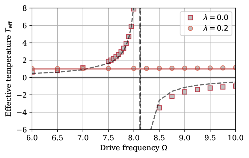
Figure S3: Effective temperature (symbols) as a function of drive frequency for the isolated model ($\lambda=0.0$) and the dissipative one ($\lambda=0.2$). In the former, the effective temperature diverges as $(\Omega^{*}-\Omega)^{-1}$ (dashed line). The divergence at $\Omega=\Omega^{*}$ signals the resonant thermalization, while the negative effective temperature for $\Omega>\Omega^{*}$ signals the population inversion Peronaci et al. (2018). In contrast, the dissipative model has temperature $\simeq T_{\text{bath}}$ (solid line) fixed by the thermal reservoir.

Here $K_{0}=\sum(V_{ij}/V)c_{i\sigma}^{\dagger}c_{j\sigma}(n_{i\bar{\sigma}}n_{j\bar{\sigma}}+\bar{n}_{i\bar{\sigma}}\bar{n}_{j\bar{\sigma}})$ are those hopping terms in Eq. (1) that do not alter the number of doubly occupied sites ($\bar{n}_{i\sigma}=1-n_{i\sigma}$, $\bar{\uparrow}=\downarrow$ and $\bar{\downarrow}=\uparrow$). Eq. (3) can be interpreted as a Hamiltonian of doublons and holons, where the first term contains hopping and the second term acts as a chemical potential. The numerical results around $\Omega^{*}\simeq U_{0}$ in the isolated model are qualitatively captured in terms of thermalization to this effective Hamiltonian. Indeed, we can extract the effective temperature $T_{\text{eff}}(\Omega)\simeq(U_{0}-\Omega)^{-1}$ (see Supplemental Material Note (1) Fig. S3) and, since $\lvert T_{\mathrm{eff}}\rvert\gg V$ for $\Omega\simeq\Omega^{*}$, we can disregard the kinetic term in Eq. (3) and calculate $\mathcal{D}=0.5[1+\exp(0.5(U_{0}-\Omega)/T_{\text{eff}})]^{-1}\simeq 0.25-(\Omega-U_{0})^{2}$. This captures the quadratic behavior for $\lambda=0.0$ (Fig. 1c; dashed line) with finite-hopping corrections responsible for the quantitative mismatch.

We now turn to the dissipative model. Here two observations are crucial. First, the enhancement of double occupancy is most pronounced for weak bath coupling (see Fig. 1e). Second, the dissipation leaves largely unchanged the spectral function of the system, while it profoundly changes its occupation (see Fig. 2). On this basis, we argue that at weak coupling the bath does not change the Floquet Hamiltonian, but only affects the effective temperature $T_{\text{eff}}\simeq T_{\text{bath}}=1$ (see Supplemental Material Note (1) Fig. S3). This leads to $\mathcal{D}\simeq 0.25+(\Omega-U_{0})$ which qualitatively reproduces the behavior for $\lambda=0.2$ around $\Omega\simeq\Omega^{*}$ (Fig. 1c; dashed line) where again the mismatch is due to the finite hopping in Eq. (3).

The outcome of this analysis is that, at least for moderately high temperatures $T_{\text{bath}}\simeq V$, the driven-dissipative protocol of Eqs. (1) and (2) leads at long times to thermal states of the doublon Hamiltonian (3). Singly occupied sites, which are relevant in the transient dynamics during doublon-holon proliferation, are not relevant for the steady-state physics, and can be considered as a reservoir of energy and particles to the doublon-holon system.

A natural question now is whether the enhanced local pairing correlations can propagate through the lattice giving a superfluid state of doublons. To answer this, we consider the next order in the Floquet Hamiltonian Note (1):

$$\bar{H}_{\text{Hub}}^{\mathrm{eff}(1)}=(-i\mathcal{J}_{1}(\tfrac{\delta U}{\Omega})VK_{+}+\text{H.c.})+\tfrac{V^{2}}{\Omega}(\mathcal{J}_{0}(\tfrac{\delta U}{\Omega}))^{2}[K_{+},K_{-}].$$ (4)

Here $\mathcal{J}_{n}(x)$ is the $n$-th order Bessel function of the first kind, $K_{+}=\sum(V_{ij}/V)c_{i\sigma}^{\dagger}c_{j\sigma}n_{i\bar{\sigma}}\bar{n}_{j\bar{\sigma}}=(K_{-})^{\dagger}$ and one has to note that, in the case of weak drive amplitude considered here, $\mathcal{J}_{n}(\delta U/\Omega)\sim(\delta U/\Omega)^{n}$ and therefore all terms in Eq. (4) indeed vanish as the inverse drive frequency.

The first two terms in parentheses in Eq. (4) create or annihilate doublon excitations, controlling the transient dynamics. However, these processes are largely inhibited in the steady state. Indeed, these terms depend strongly on the drive amplitude $\delta U$, which controls the transient time-scale but does not influence the long-time steady-state, as found in both the isolated Peronaci et al. (2018) and the dissipative models (see Supplementary Material Note (1) Sec. V).

The last term in Eq. (4) is similar to the Schrieffer-Wolff result Bukov et al. (2016); MacDonald et al. (1988), which is retrieved for $\delta U\rightarrow 0$ at fixed $\Omega=U_{0}$. It contains several contributions such as density and exchange interactions, and correlated three-site hopping processes. At equilibrium and half filling, in the relevant limit of zero double occupancy, this gives the usual anti-ferromagnetic Heisenberg model. In far-from-equilibrium situations, if a sizeable population of doublons is achieved as in the present case, the same term leads to a completely different physics (see also Ref. Rosch et al. (2008)).

To discuss Hamiltonian (4) on states with very large double occupancy, it is instructive to neglect processes involving singly occupied sites and rewrite it as Note (1):

$$\bar{H}_{\text{Hub}}^{\mathrm{eff}}=J_{\text{eff}}\sum\nolimits_{\braket{ij}}(c_{i\uparrow}^{\dagger}c_{i\downarrow}^{\dagger}c_{j\downarrow}c_{j\uparrow}+n_{i\uparrow}n_{i\downarrow}\bar{n}_{j\uparrow}\bar{n}_{j\downarrow}).$$ (5)

Here $J_{\text{eff}}=2V^{2}/\Omega(\mathcal{J}_{0}(\delta U/\Omega))^{2}$, the first term is a doublon hopping, and the second term a first-neighbor doublon interaction. It is now convenient to consider a transformation on spin-down operators $c_{i\downarrow}\rightarrow\tilde{c}_{i\downarrow}=(-1)^{i}c_{i\downarrow}^{\dagger}$ which recasts Eq. (5) as $\bar{H}_{\text{Hub}}^{\mathrm{eff}}=-J_{\text{eff}}\sum\bm{\eta}_{i}\cdot\bm{\eta}_{j}$ namely as an isotropic ferromagnetic Heisenberg model for the so-called $\eta$-spins $\bm{\eta}_{i}=\frac{1}{2}\sum_{\alpha\beta}\tilde{c}_{i\alpha}^{\dagger}\bm{\sigma}_{\alpha\beta}\tilde{c}_{i\beta}$ Note (1). The invariance under $\eta$-spin rotation is associated to the charge SU${}_{\text{C}}$(2) symmetry of Hamiltonian (1) which can be used to build eigenstates of the Hubbard model with staggered long-range superconducting correlations ($\eta$-pairing) Yang (1989); Zhang (1990). These same correlations are encoded in Eq. (5). Indeed, the $\eta$-spin ferromagnetic Heisenberg model has magnetization $\braket{\eta^{z}}=\mathcal{D}-0.5$ and below a critical temperature $\sim J_{\text{eff}}$ it has finite order parameter in the $xy$-plane, which corresponds to staggered long-range pairing correlations $\braket{c^{\dagger}_{i\uparrow}c^{\dagger}_{i\downarrow}+\text{H.c.}}=(-1)^{i}\braket{2\eta_{i}^{x}}=(-1)^{i}\sqrt{4\mathcal{D}(1-\mathcal{D})}$.

We stress again that here, for simplicity, we do not consider the interplay between doublons and singly occupied sites, which would result in additional terms in Eq. (5). Moreover, we notice that the SU${}_{\text{C}}(2)$ symmetry implies a degeneracy between the $xy$-plane and the $z$-axis of the $\eta$-spin, which translates into a competition between superfluidity and charge-density wave. We leave the investigation of these issues for future work.

The model system investigated here can be realized in current experimental platforms. Particularly promising are Mott-insulating organic molecular crystals, where laser excitations can induce an effective time-periodic modulation of interaction Kawakami et al. (2009); Singla et al. (2015). More direct control is achieved with ultracold atoms in optical lattices. Recent experiments Messer et al. (2018); Sandholzer et al. (2019) have studied the Floquet prethermal state and remarkably found large double occupancy for drive above resonance. We suggest that also in these cases a key role is played by dissipation, which is unavoidable even in cold atoms. Finally, we notice that these experiments have focused on the regime where the effective Hamiltonian reduces to a renormalized Hubbard model. In contrast, here we have studied the case of a doublon-only Floquet Hamiltonian. Therefore, we suggest future experiments to investigate this latter regime to detect the presence of staggered pairing correlations.

Conclusions – In this work, we have studied the combination of a periodically driven interaction and a dissipative bath in the strongly repulsive Fermi-Hubbard model. For weak bath coupling and frequency in a range above the resonance of the isolated model Peronaci et al. (2018), we find a large increase of double occupancy, well above the maximum equilibrium value, which we interpret as an enhancement of local pairing correlations, and understand in terms of thermalization to the lowest-order Floquet Hamiltonian.

Remarkably, the next-order Floquet Hamiltonian contains terms which promote staggered pairing correlations. Therefore, provided a nonequilibrium protocol to reach low enough effective temperatures (see e.g. Ref. Werner et al. (2019b)) and eventually further increase the doublon density, the steady state of the driven-dissipative Fermi-Hubbard model would contain off-diagonal staggered long-range order ($\eta$-pairing), hence a superfluid phase of doublon excitations, similarly to what very recently found in similar models Werner et al. (2019a); Li et al. (2019).

Supplemental Material

I I. NCA with bosonic bath

Here we describe our implementation of a bosonic bath in the non-crossing-approximation (NCA) impurity solver for non-equilibrium dynamical mean-field theory (DMFT). Starting from Hamiltonians (1) and (2) in main text, we integrate out the bosons and obtain the action:

$$\small\begin{split}S_{\text{latt}}&=\int\text{d}t\,\sum_{ij,\sigma}V_{ij}c^{\dagger}_{i\sigma}(t)c_{j\sigma}(t)\\ &+\int\text{d}t\,U(t)\sum_{i}(n_{i\uparrow}(t)-\tfrac{1}{2})(n_{i\downarrow}(t)-\tfrac{1}{2})\\ &+\lambda^{2}\int\int\text{d}t\,\text{d}t^{\prime}\,\Delta_{b}(t,t^{\prime})\sum_{i}(n_{i}(t)-1)(n_{i}(t^{\prime})-1).\end{split}$$ (S1)

Here the integrals are along the three-branch Keldysh contour and the bath enters via the hybridization $\Delta_{b}(t,t^{\prime})=-i\int\text{d}\omega\,J(\omega)(\theta(t,t^{\prime})+n_{B}(\omega/T_{\text{bath}}))e^{-i\omega(t-t^{\prime})}$ where $\theta(t,t^{\prime})$ is the Heaviside theta function on contour and $n_{b}(\omega)$ is the Bose distribution.

In DMFT the lattice action (S1) is mapped onto the action of a quantum impurity coupled to a self-consistent fermionic bath:

$$\small\begin{split}S_{\text{imp}}&=\int\text{d}t\,U(t)(n_{\uparrow}(t)-\tfrac{1}{2})(n_{\downarrow}(t)-\tfrac{1}{2})\\ &+V^{2}\int\int\text{d}t\,\text{d}t^{\prime}\,G(t,t^{\prime})\sum_{\sigma}c_{\sigma}^{\dagger}(t)c_{\sigma}(t^{\prime})\\ &+\lambda^{2}\int\int\text{d}t\,\text{d}t^{\prime}\,\Delta_{b}(t,t^{\prime})(n(t)-1)(n(t^{\prime})-1).\end{split}$$ (S2)

Here we have used the relation $\Delta(t,t^{\prime})=V^{2}G(t,t^{\prime})$ for the hybridization $\Delta(t,t^{\prime})$ of the self-consistent fermionic bath, which is valid on Bethe lattice.

To derive the NCA equations, we expand the partition function $\text{Tr}(\exp[-iS_{\text{imp}}])$ into a power series in $V$ and $\lambda$ and truncate the expansion at the first self-consistent order Eckstein and Werner (2010); Rüegg et al. (2013); Chen et al. (2016). This series is expressed in terms of the propagator of the states of the impurity $R$, and of its self-energy $S$, which satisfy an integro-differential equation similar to the usual Dyson equation (see Ref. Peronaci et al. (2018) for our implementation). Then, in the present case a convenient basis choice is $\{\ket{0},\ket{\uparrow},\ket{\downarrow},\ket{\uparrow\downarrow}\}$ which makes the propagator $R$ and the self-energy $S$ diagonal. Finally, we exploit the spin SU$(2)$ symmetry and the particle-hole SU${}_{\text{C}}(2)$ symmetry of Eq. (S2) which further reduce the number of propagators to two: one for the empty state $\ket{0}$ and one for the singly-occupied state $\ket{\uparrow}$, with the following self-energies:

$$\small S_{\ket{0}}(t,t^{\prime})= -2iR_{\ket{\uparrow}}(t,t^{\prime})\Delta(t^{\prime},t)$$ (S3)

$$+i\lambda^{2}R_{\ket{0}}(t,t^{\prime})(\Delta_{b}(t,t^{\prime})+\Delta_{b}(t^{\prime},t)),$$

$$S_{\ket{\uparrow}}(t,t^{\prime})= +2iR_{\ket{0}}(t,t^{\prime})\Delta(t,t^{\prime}).$$ (S4)

II. OCA benchmark

In this work we investigate the Mott-insulating phase of the Fermi-Hubbard model with average interaction parameter $U_{0}=8V$ much larger than the bare band-width $W=4V$. Moreover, we consider initial thermal density matrix at a rather high temperature $T=1$. In these conditions, the NCA approximation is expected to perform well both at equilibrium and out of equilibrium Eckstein and Werner (2010).

To confirm this, we have performed some calculations using the next-order one-crossing approximation (OCA). This takes into consideration terms of order $\mathcal{O}(V^{4})$ in the hybridization expansion Eckstein and Werner (2010); Rüegg et al. (2013) (see Ref. Peronaci et al. (2018) for our implementation). As expected, the time evolution of double occupancy and kinetic energy (Fig. S1) is essentially identical to the one shown in the main text (Fig. 1a-b).

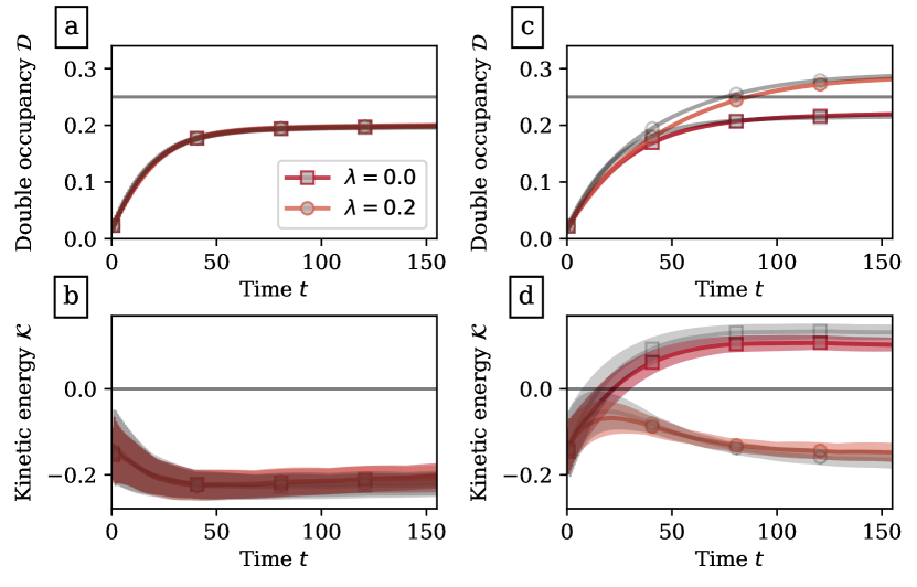
Figure S1: Time evolution of double occupancy and kinetic energy using the OCA impurity solver for DMFT: Isolated model ($\lambda=0$) and dissipative model ($\lambda=0.2$) for drive frequency below resonance $\Omega=7$ (a-b) and above resonance $\Omega=9$ (c-d). Legend in (a) is common to (a-b-c-d). Light grey curves are the corresponding NCA results, for comparison.

III. Fermionic bath

It is interesting to consider an external reservoir of fermionic modes, instead of the bosonic bath considered in the main text. To do so, we substitute Eq. (2) of the main text with the following coupling to a fermionic bath:

$$\small H_{\text{diss}}=\sum_{i\alpha}\omega_{\alpha}f^{\dagger}_{i\alpha}f_{i\alpha}+\lambda\sum_{i\sigma\alpha}(g_{\alpha}c_{i\sigma}^{\dagger}f_{i\alpha}+g_{\alpha}^{*}f_{i\alpha}^{\dagger}c_{i\sigma}).$$ (S5)

Here the operators $f$’s represent sets of independent fermionic harmonic oscillators. In this case, the system can dissipate both energy and particles. Moreover, this type of coupling can be treated exactly: integrating out the fermionic bath, we introduce an additional hybridization $\Delta_{f}(t,t^{\prime})$ which can simply be added to the DMFT self-consistent hybridization $\Delta(t,t^{\prime})$.

As shown in Fig. S2, the coupling with a fermionic bath does not lead to the same interesting features discussed in the main text for the bosonic bath (cf. Fig. 1a-c). This is due to the fact that the bosonic bath, as opposed to the fermionic bath, commutes with the local density and conserves double occupancy, and therefore it preserves the mechanism for Floquet prethermalization.

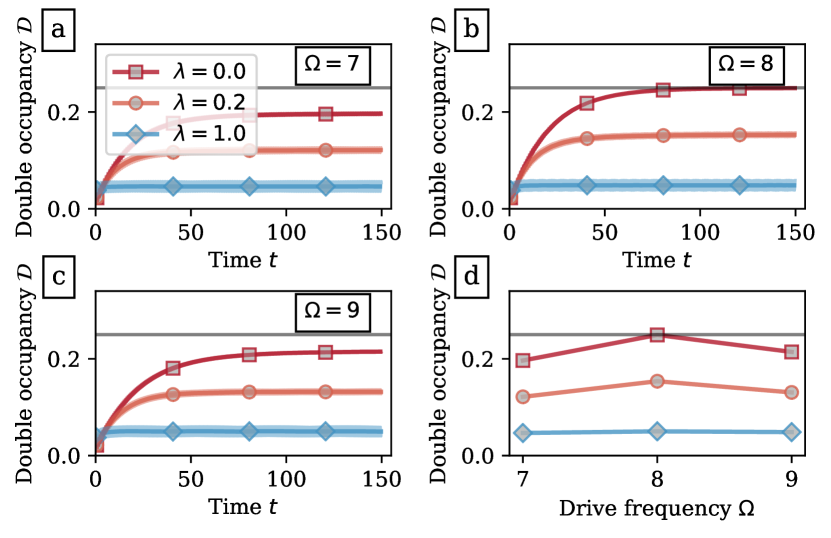
Figure S2: Panels (a-b-c): Time evolution of double occupancy for the isolated model ($\lambda=0.0$) and the dissipative one with fermionic bath ($\lambda=0.2,1.0$) for various drive frequencies. Legend in (a) is common to (a-b-c-d). Panel (d): Long-time average of double occupancy as a function of drive frequency.

IV. Effective temperature

In Fig. 2 of main text we show the steady-state average distribution function $\bar{F}(\omega)$ for $\Omega=9>\Omega^{*}$, along with a Fermi-function fit $[1+\exp(\omega/T_{\text{eff}})]^{-1}$ around the center of the upper Hubbard band $\omega\simeq U_{0}/2$. From this fit we can extract the effective temperature $T_{\text{eff}}$. Here, in Fig. S2 we plot this effective temperature for the isolated and the dissipative models, as a function of the drive frequency.

V. Rotating-frame transformation and high-frequency expansion

To carry out the large-frequency expansion Bukov et al. (2015a, 2016), we first need to transform Hamiltonian (1) of main text to a rotating frame with respect to the interaction:

$$H_{\text{Hub}}(t) =\sum V_{ij}c^{\dagger}_{i\sigma}c_{j\sigma}+U(t)\sum\nolimits_{i}(n_{i\uparrow}-\tfrac{1}{2})(n_{i\downarrow}-\tfrac{1}{2}),$$ (S6)

$$\bar{H}_{\text{Hub}}(t) =e^{S(t)}(H_{\text{Hub}}(t)-i\partial_{t})e^{-S(t)},$$ (S7)

$$S(t) =iF(t)\sum\nolimits_{i}(n_{i\uparrow}-\tfrac{1}{2})(n_{i\downarrow}-\tfrac{1}{2})=iF(t)D,$$ (S8)

$$F(t) =\Omega t-(\delta U/\Omega)\cos\Omega t.$$ (S9)

It is useful to introduce the operators $K_{0}$ and $K_{\pm}$ as in the main text ($\bar{n}_{i\sigma}=1-n_{i\sigma}$, $\bar{\uparrow}=\downarrow$ and $\bar{\downarrow}=\uparrow$):

$$K_{0} =\sum\nolimits_{ij\sigma}(V_{ij}/V)c_{i\sigma}^{\dagger}c_{j\sigma}(n_{i\bar{\sigma}}n_{j\bar{\sigma}}+\bar{n}_{i\bar{\sigma}}\bar{n}_{j\bar{\sigma}}),$$ (S10)

$$K_{+} =\sum\nolimits_{ij\sigma}(V_{ij}/V)c_{i\sigma}^{\dagger}c_{j\sigma}n_{i\bar{\sigma}}\bar{n}_{j\bar{\sigma}}=(K_{-})^{\dagger}.$$ (S11)

It is easy to verify that $\sum V_{ij}c^{\dagger}_{i\sigma}c_{j\sigma}=V(K_{0}+K_{+}+K_{-})$. Then, using $[D,K_{0}]=0$ and $[D,K_{+}]=\pm K_{\pm}$ we find:

$$\small\begin{split}\bar{H}_{\text{Hub}}(t)&=V(K_{0}+e^{iF(t)}K_{+}+e^{-iF(t)}K_{-})\\ &+(U_{0}-\Omega)\sum\nolimits_{i}(n_{i\uparrow}-\tfrac{1}{2})(n_{i\downarrow}-\tfrac{1}{2}).\end{split}$$ (S12)

The rotated Hamiltonian maintains the $2\pi/\Omega$-periodicity. Its Fourier components contain the Bessel function of the first kind $\int_{0}^{2\pi}\text{d}\tau\,\exp(i(x\cos\tau-m\tau))=2\pi i^{m}\mathcal{J}_{m}(x)$ through the following expansions:

$$e^{iF(t)}=\sum\nolimits_{m}(-i)^{1+m}\mathcal{J}_{1+m}(\tfrac{\delta U}{\Omega})e^{-im\Omega t},$$ (S13)

$$e^{-iF(t)}=\sum\nolimits_{m}i^{1-m}\mathcal{J}_{1-m}(\tfrac{\delta U}{\Omega})e^{-im\Omega t}.$$ (S14)

In particular, the average Hamiltonian and the first Fourier components read:

$$\bar{H}_{\text{Hub}}^{(0)} =VK_{0}-i\mathcal{J}_{1}(\tfrac{\delta U}{\Omega})VK_{+}+i\mathcal{J}_{1}(\tfrac{\delta U}{\Omega})VK_{-}$$ (S15a)

$$+(U_{0}-\Omega)\sum\nolimits_{i}(n_{i\uparrow}-\tfrac{1}{2})(n_{i\downarrow}-\tfrac{1}{2}),$$

$$\bar{H}_{\text{Hub}}^{(1)} =-\mathcal{J}_{2}(\tfrac{\delta U}{\Omega})VK_{+}+\mathcal{J}_{0}(\tfrac{\delta U}{\Omega})VK_{-},$$ (S15b)

$$\bar{H}_{\text{Hub}}^{(-1)} =\mathcal{J}_{0}(\tfrac{\delta U}{\Omega})VK_{+}-\mathcal{J}_{2}(\tfrac{\delta U}{\Omega})VK_{-}.$$ (S15c)

I.1 Eqs. (3) and (4) of main text

Here we calculate the first two terms of the (van-Vleck) large-frequency expansion, with general expression Bukov et al. (2016):

$$\small H_{F}=H_{0}+\sum_{m>0}\frac{[H_{-m},H_{m}]}{m\Omega}+\mathcal{O}(\tfrac{1}{\Omega^{2}}).$$ (S16)

The Fourier components $H_{m}$ are given in Eqs. (S15) and depend on frequency through the Bessel function. When the large-frequency limit is taken at fixed $\delta U/\Omega$, this dependence does not show up in the expansion. In contrast, here we keep $\delta U$ constant and we have to consider the asymptotic behavior $\mathcal{J}_{n}(\delta U/\Omega)\sim(\delta U/\Omega)^{n}$. Then, there are terms in the average Hamiltonian (S15a) which vanish as $\Omega^{-1}$ and do not enter the lowest order of the expansion (cf. Eq. (3) of main text):

$$\small\bar{H}_{\text{Hub}}^{\text{eff}(0)}=VK_{0}+(U_{0}-\Omega)\sum\nolimits_{i}(n_{i\uparrow}-\tfrac{1}{2})(n_{i\downarrow}-\tfrac{1}{2}).$$ (S17)

For the same reason, at first order only enter those terms which actually vanish as $\Omega^{-1}$ (cf. Eq. (4) of main text):

$$\small\bar{H}_{\text{Hub}}^{\mathrm{eff}(1)}=(-i\mathcal{J}_{1}(\tfrac{\delta U}{\Omega})VK_{+}+\text{H.c.})+\tfrac{V^{2}}{\Omega}(\mathcal{J}_{0}(\tfrac{\delta U}{\Omega}))^{2}[K_{+},K_{-}].$$ (S18)

I.2 Eq. (5) of main text

Here we calculate the commutator in Eq. (S18):

$$\small\begin{split}[K_{+},K_{-}]&=\sum_{ij\sigma}\sum_{kl\sigma^{\prime}}[c_{i\sigma}^{\dagger}c_{j\sigma}n_{i\bar{\sigma}}\bar{n}_{j\bar{\sigma}},c_{k\sigma^{\prime}}^{\dagger}c_{l\sigma^{\prime}}\bar{n}_{k\bar{\sigma}^{\prime}}n_{l\bar{\sigma}^{\prime}}]\\ &=\sum_{ij\sigma}\sum_{kl\sigma^{\prime}}[c_{i\sigma}^{\dagger}c_{j\sigma},c_{k\sigma^{\prime}}^{\dagger}c_{l\sigma^{\prime}}]n_{i\bar{\sigma}}\bar{n}_{j\bar{\sigma}}\bar{n}_{k\bar{\sigma}^{\prime}}n_{l\bar{\sigma}^{\prime}}\\ &+\sum_{ij\sigma}\sum_{kl\sigma^{\prime}}c_{k\sigma^{\prime}}^{\dagger}c_{l\sigma^{\prime}}[c_{i\sigma}^{\dagger}c_{j\sigma},\bar{n}_{k\bar{\sigma}^{\prime}}n_{l\bar{\sigma}^{\prime}}]n_{i\bar{\sigma}}\bar{n}_{j\bar{\sigma}}\\ &+\sum_{ij\sigma}\sum_{kl\sigma^{\prime}}c_{i\sigma}^{\dagger}c_{j\sigma}[n_{i\bar{\sigma}}\bar{n}_{j\bar{\sigma}},c_{k\sigma^{\prime}}^{\dagger}c_{l\sigma^{\prime}}]\bar{n}_{k\bar{\sigma}^{\prime}}n_{l\bar{\sigma}^{\prime}}.\end{split}$$ (S19)

The commutators in Eq. (S19) give three- and two-site terms. If we retain only the two-site terms, then the first sum in Eq. (S19) reads:

$$\small\sum\nolimits_{ij}(n_{i\sigma}n_{i\bar{\sigma}}\bar{n}_{j\bar{\sigma}}-n_{j\sigma}n_{i\bar{\sigma}}\bar{n}_{j\bar{\sigma}})=\sum\nolimits_{ij}(n_{i\sigma}-n_{j\sigma})n_{i\bar{\sigma}}\bar{n}_{j\bar{\sigma}}.$$ (S20)

Now, with the identities $c_{i\sigma}n_{i\sigma}=c_{i\sigma}$ and $n_{i\sigma}c_{i\sigma}=0$, together with their Hermitian conjugates, it is easy to see that the terms in the second sum in Eq. (S19) are non-vanishing only if $\{i=l,j=k,\sigma^{\prime}=\bar{\sigma}\}$, giving:

$$\small\begin{split}&\sum\nolimits_{ij}c_{j\sigma}^{\dagger}c_{i\sigma}(-c_{i\bar{\sigma}}^{\dagger}c_{j\bar{\sigma}}n_{i\bar{\sigma}}-\bar{n}_{j\bar{\sigma}}c_{i\bar{\sigma}}^{\dagger}c_{j\bar{\sigma}})\\ &=\sum\nolimits_{ij}c_{i\bar{\sigma}}^{\dagger}c_{i\sigma}c_{j\sigma}^{\dagger}c_{j\bar{\sigma}}\\ &=\sum\nolimits_{ij}(c_{i\uparrow}^{\dagger}c_{i\downarrow}c_{j\downarrow}^{\dagger}c_{j\uparrow}+c_{i\downarrow}^{\dagger}c_{i\uparrow}c_{j\uparrow}^{\dagger}c_{j\downarrow})\\ &=\sum\nolimits_{ij}(S_{i}^{+}S_{j}^{-}+S_{i}^{-}S_{j}^{+})=2\sum\nolimits_{ij}(S_{i}^{x}S_{j}^{x}+S_{i}^{y}S_{j}^{y}).\end{split}$$ (S21)

Analogously, terms in the third sum in Eq. (S19) are non-vanishing only if $\{i=k,j=l,\sigma^{\prime}=\bar{\sigma}\}$, giving:

$$\small\begin{split}&\sum\nolimits_{ij}c_{i\sigma}^{\dagger}c_{j\sigma}(n_{i\bar{\sigma}}c_{i\bar{\sigma}}^{\dagger}c_{j\bar{\sigma}}+c_{i\bar{\sigma}}^{\dagger}c_{j\bar{\sigma}}\bar{n}_{j\bar{\sigma}})\\ &=\sum\nolimits_{ij}c_{i\sigma}^{\dagger}c_{j\sigma}c_{i\bar{\sigma}}^{\dagger}c_{j\bar{\sigma}}=2\sum\nolimits_{ij}c_{i\uparrow}^{\dagger}c_{i\downarrow}^{\dagger}c_{j\downarrow}c_{j\uparrow}.\end{split}$$ (S22)

To proceed, we restrict ourselves to a subspace with double occupancy so large that we can neglect singly occupied sites. In other words, we restrict ourselves to the local subspace $\{\ket{0},\ket{\uparrow\downarrow}\}$. Within this subspace we have $n_{i\sigma}=n_{i\bar{\sigma}}$ so that Eq. (S20) simplifies to:

$$\small\sum\nolimits_{ij}n_{i\sigma}\bar{n}_{j\bar{\sigma}}=\sum\nolimits_{ij}n_{i\sigma}n_{i\bar{\sigma}}\bar{n}_{j\bar{\sigma}}\bar{n}_{j\sigma}=2\sum\nolimits_{ij}n_{i\uparrow}n_{i\downarrow}\bar{n}_{j\downarrow}\bar{n}_{j\uparrow}.$$ (S23)

Moreover, within this subspace Eq. (S21) vanishes, so that the final result reads (cf. Eq. (5) of main text):

$$\small 2\tfrac{V^{2}}{\Omega}(\mathcal{J}(\tfrac{\delta U}{\Omega}))^{2}\sum\nolimits_{ij}(c_{i\uparrow}^{\dagger}c_{i\downarrow}^{\dagger}c_{j\downarrow}c_{j\uparrow}+n_{i\uparrow}n_{i\downarrow}\bar{n}_{j\downarrow}\bar{n}_{j\uparrow}).$$ (S24)

This reproduces Eq.(2) of Ref. Rosch et al. (2008) for $\delta U=0$, $\Omega=U_{0}$.

I.3 $\eta$-spin ferromagnetic Heisenberg

To recast Eq. (S24) to the ferromagnetic Heisenberg model considered in the main text, we carry out a transformation on the spin-down only:

$$c_{i\uparrow} \rightarrow\tilde{c}_{i\uparrow}=c_{i\uparrow},$$ (S25)

$$c_{i\downarrow} \rightarrow\tilde{c}_{i\downarrow}=(-1)^{i}c_{i\downarrow}^{\dagger}.$$ (S26)

Here $(-1)^{i}=\pm 1$ on different sublattices of a bipartite lattice. Then the first term in Eq. (S24) transforms to:

$$\small\begin{split}-&\sum\nolimits_{ij}(\tilde{c}_{i\uparrow}^{\dagger}\tilde{c}_{i\downarrow}\tilde{c}_{j\downarrow}^{\dagger}\tilde{c}_{j\uparrow}+\tilde{c}_{i\downarrow}^{\dagger}\tilde{c}_{i\uparrow}\tilde{c}_{j\uparrow}^{\dagger}\tilde{c}_{j\downarrow})\\ =&-\sum\nolimits_{ij}(\eta_{i}^{+}\eta_{j}^{-}+\eta_{i}^{-}\eta_{j}^{+})=-2\sum\nolimits_{ij}(\eta_{i}^{x}\eta_{j}^{x}+\eta_{i}^{y}\eta_{j}^{y}).\end{split}$$ (S27)

This has the same form of Eq. (S21) with the additional minus sign $(-1)^{i+j}=-1$ for nearest-neighbor sites. The $\eta$-spin has the same definition of the physical spin for the transformed electrons $\bm{\eta}_{i}=\frac{1}{2}\sum_{\alpha\beta}\tilde{c}_{i\alpha}^{\dagger}\bm{\sigma}_{\alpha\beta}\tilde{c}_{i\beta}$ where $\bm{\sigma}$ is the vector of the three Pauli matrices:

$$\small\begin{split}\eta_{i}^{x}&=\frac{\tilde{c}_{i\uparrow}^{\dagger}\tilde{c}_{i\downarrow}+\tilde{c}_{i\downarrow}^{\dagger}\tilde{c}_{i\uparrow}}{2},\\ \eta_{i}^{y}&=\frac{\tilde{c}_{i\uparrow}^{\dagger}\tilde{c}_{i\downarrow}-\tilde{c}_{i\downarrow}^{\dagger}\tilde{c}_{i\uparrow}}{2i},\\ \eta_{i}^{z}&=\frac{\tilde{c}_{i\uparrow}^{\dagger}\tilde{c}_{i\uparrow}-\tilde{c}_{i\downarrow}^{\dagger}\tilde{c}_{i\downarrow}}{2}.\end{split}$$ (S28)

Additionally, if one defines $\eta_{i}^{+}=\tilde{c}_{i\uparrow}^{\dagger}\tilde{c}_{i\downarrow}$ and $\eta_{i}^{-}=\tilde{c}_{i\downarrow}^{\dagger}\tilde{c}_{i\uparrow}$ then $\eta_{i}^{x}=(\eta_{i}^{+}+\eta_{i}^{-})/2$ and $\eta_{i}^{y}=(\eta_{i}^{+}-\eta_{i}^{-})/2$.

To consider the second term in Eq. (S24), we notice that under the transformation (S25) the density operator transforms as $n_{i\uparrow}\rightarrow\tilde{n}_{i\uparrow}=n_{i\uparrow}$ and $n_{i\downarrow}\rightarrow\tilde{n}_{i\downarrow}=1-n_{i\downarrow}$. Then, this term transforms to (keep in mind that in the considered subspace $n_{i\sigma}=n_{i\bar{\sigma}}$):

$$\small 2\sum\nolimits_{ij}\tilde{n}_{i\bar{\sigma}}\tilde{n}_{j\sigma}=\sum\nolimits_{ij}(\tilde{n}_{i\uparrow}\tilde{n}_{j\downarrow}+\tilde{n}_{i\downarrow}\tilde{n}_{j\uparrow})=-2\sum\nolimits_{ij}(\eta_{i}^{z}\eta_{j}^{z}-\tfrac{1}{4}).$$ (S29)

The last equality is best demonstrated verifying that the operators have the same matrix elements in the considered subspace. Alternatively, an explicit derivation reads:

$$\small\begin{split}&\tilde{n}_{i\uparrow}\tilde{n}_{j\downarrow}+\tilde{n}_{i\downarrow}\tilde{n}_{j\uparrow}\\ &=\tfrac{1}{2}(\tilde{n}_{i\uparrow}\tilde{n}_{j\downarrow}+\tilde{n}_{i\downarrow}\tilde{n}_{j\uparrow})+\tfrac{1}{2}(\tilde{n}_{i\uparrow}\tilde{n}_{j\downarrow}+\tilde{n}_{i\downarrow}\tilde{n}_{j\uparrow})\\ &=\tfrac{1}{2}(\tilde{n}_{i\uparrow}\tilde{n}_{j\downarrow}+\tilde{n}_{i\downarrow}\tilde{n}_{j\uparrow})+\tfrac{1}{2}(\tilde{n}_{i\uparrow}(1-\tilde{n}_{j\uparrow})+\tilde{n}_{i\downarrow}(1-\tilde{n}_{j\downarrow}))\\ &=-2(\tfrac{1}{4}(\tilde{n}_{i\uparrow}-\tilde{n}_{i\downarrow})(\tilde{n}_{j\uparrow}-\tilde{n}_{j\downarrow})-\tfrac{1}{4}).\end{split}$$

Here it is crucial the use of $\tilde{n}_{i\uparrow}+\tilde{n}_{i\downarrow}=1$.

VI. Role of drive amplitude

In Fig. S4 we compare the time evolutions for various drive amplitudes $\delta U$. These show interesting features in both the isolated model (see also Ref. Peronaci et al. (2018)) and the dissipative model. First, it is evident how the drive amplitude controls the time scale of the transient dynamics, with larger amplitudes inducing shorter transients. Second, the steady steady, in sharp contrast, appears to be largely independent from the drive amplitude.

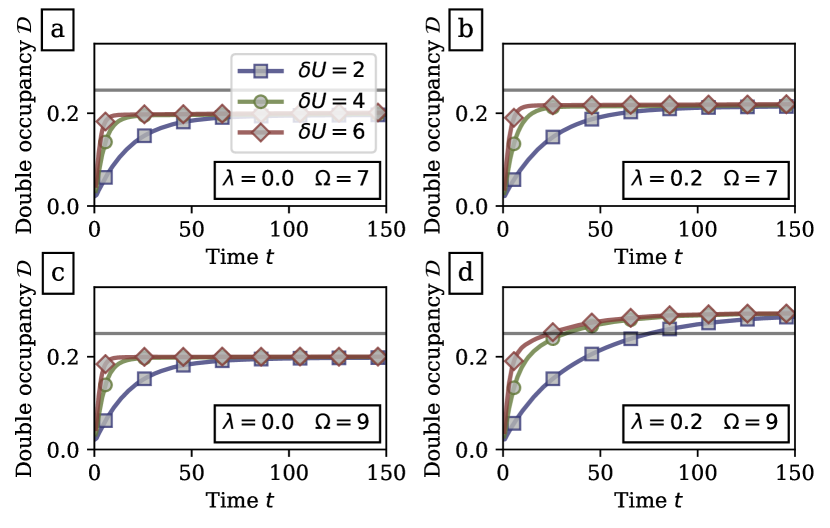
Figure S4: Time evolution of double occupancy for the isolated model ($\lambda=0.0$) and the dissipative one ($\lambda=0.2$), for drive frequencies below ($\Omega=7$) and above ($\Omega=9$) resonance, and for different drive amplitude $\delta U=2,4,6$.

These observations are consistent with and provide further validation to our analysis based on the Floquet theory (Eqs. (3) to (5) of main text). Indeed, in Eq. (4) a factor $\mathcal{J}_{1}(\delta U/\Omega)\sim\delta U/\Omega$ multiplies the terms creating doublon excitations, which are responsible for the increase of double occupancy in the transient dynamics. Thus, a large drive amplitude enhances these terms and makes the transient shorter. Moreover, since the long-time values do not depend on $\delta U$, it is confirmed that these terms are largely suppressed in the steady state, which validates the introduction of the doublon-only Hamiltonian (5).

VII. Hypercubic lattice

In the main text we consider a system on Bethe lattice, whose free-electron density of states is semicircular. Here we consider a hypercubic lattice in infinite dimensions, whose free-electron density of states is Gaussian. In Fig. S5 we show that this difference does not qualitatively affect the physics discussed in the main text. For drive frequency above resonance $\Omega=9>\Omega^{*}\simeq U_{0}$ we observe qualitatively the same increase in the long-time double occupancy which goes above $0.25$ in the dissipative model ($\lambda=0.2$) both on Bethe lattice (Fig. S5a) and on hypercubic lattice (Fig. S5b).

The spectral and occupation function on hypercubic lattice also show the same changes between the isolated (Fig. S5c) and the dissipative (Fig. S5d) models. In the former, we observe population inversion within each of the Hubbard bands. In the latter, as a consequence of dissipation, the population inversion within the Hubbard bands does not take place. At the same time, the occupation of the upper Hubbard band grows larger than the one of the lower Hubbard band (cf. Fig. 2 of main text).

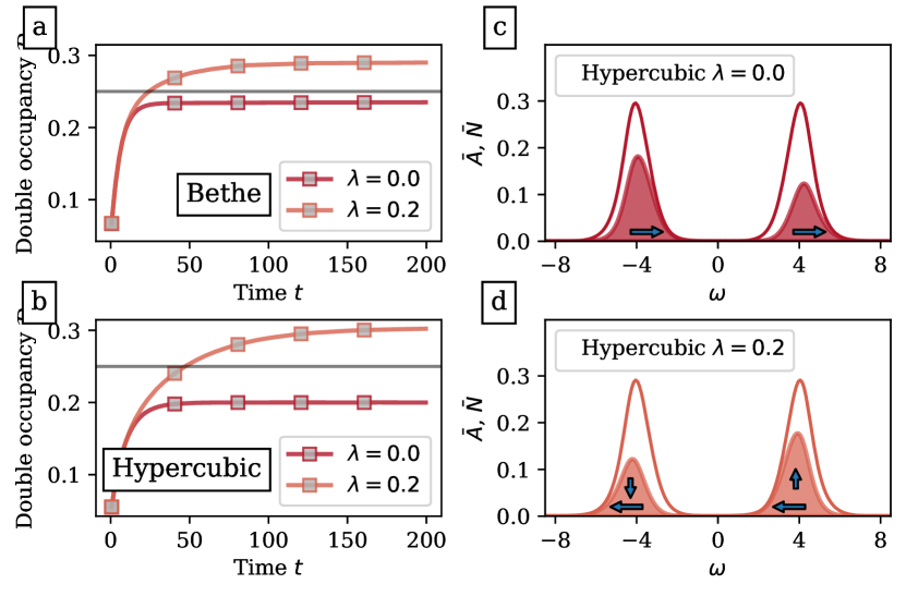
Figure S5: Time evolution of double occupancy for drive frequency $\Omega=9>\Omega^{*}\simeq U_{0}$ and amplitude $\delta U=4$ on Bethe (a) and hypercubic (b) lattices for $\lambda=0.0$ (isolated) and $\lambda=0.2$ (dissipative). Corresponding long-time average spectral function $\bar{A}(\omega)$ (solid line) and occupation function $\bar{N}(\omega)$ (filled area) for the hypercubic lattice, showing population inversion in the isolated model (c), signaled by the blueshift of $\bar{N}(\omega)$ with respect to $\bar{A}(\omega)$ (arrows); and large double occupancy in the dissipative model (d), signaled by the increase of $\bar{N}(\omega)$ in the high-energy band (vertical arrows).

VIII. Bath spectral function

In the main text we consider a bosonic thermal bath with spectral function $J(\omega)=\frac{\omega_{c}}{2}(\frac{\omega}{\omega_{c}})^{s}e^{-\frac{\omega}{\omega_{c}}}$ with $\omega_{c}=1$ and $s=2$. Here in Fig. S6 we provide additional numerical results with various parameters $\omega_{c}$ and $s$.

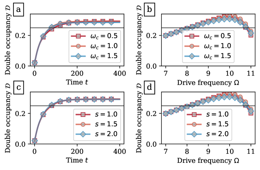
Figure S6: Time evolution for drive frequency $\Omega=9>\Omega^{*}$ and long-time average of double occupancy as a function of drive frequency for various bath parameter $\omega_{c}=0.5,1,1.5$ at fixed $s=2$ (a-b) and $s=1,1.5,2$ at fixed $\omega_{c}=1$ (c-d).