[c] 0pt

author

Stroboscopic high-order nonlinearity for quantum optomechanics

High-order quantum nonlinearity is an important prerequisite for the advanced quantum technology leading to universal quantum processing with large information capacity of continuous variables. Levitated optomechanics, a field where motion of dielectric particles is driven by precisely controlled tweezer beams, is capable of attaining the required nonlinearity via engineered potential landscapes of mechanical motion. Importantly, to achieve nonlinear quantum effects, the evolution caused by the free motion of mechanics and thermal decoherence have to be suppressed. For this purpose, we devise a method of stroboscopic application of a highly nonlinear potential to a mechanical oscillator that leads to the motional quantum non-Gaussian states exhibiting nonclassical negative Wigner function and squeezing of a nonlinear combination of mechanical quadratures. We test the method numerically by analysing highly instable cubic potential with relevant experimental parameters of the levitated optomechanics, prove its feasibility within reach, and propose an experimental test. The method paves a road for experiments instantaneously transforming a ground state of mechanical oscillators to applicable nonclassical states by nonlinear optical force.

1 Introduction

Quantum physics and technology with continuous variables (CVs) [1] has achieved noticeable progress recently. A potential advantage of CVs is the in principle unlimited energy and information capacity of single oscillator mode. In order to fully gain the benefits of CVs and to achieve universal quantum processing one requires an access to a nonlinear operation [2, 3], that is, at least a cubic potential. Additionally, the CV quantum information processing can be greatly simplified and stabilized if variable higher-order potentials are available [4]. Variability of nonlinear gates can also help to overcome limits for fault tolerance [5]. Nanomechanical systems profit from a straightforward feasible way to achieve the nonlinearity by inducing a controllable classical nonlinear force of electromagnetic nature on a linear mechanical oscillator  [6, 7, 8]. Such a nonlinear force needs to be fast, strong and controllable on demand to access different nonlinearities required for an efficient universal CV quantum processing. Therefore, the field of optomechanics [9, 10, 11, 12] is a promising candidate to provide the key element for the variable on-demand nonlinearity. Optomechanical systems have reached a truly quantum domain recently, demonstrating the effects ranging from the ground state cooling [13, 14] and squeezing [15, 16] of the mechanical motion to the entanglement of distant mechanical oscillators [17, 18]. Of particular interest are the levitated systems in which the potential landscape of the mechanical motion is provided by a highly developed device — an optical tweezer [19, 20, 21, 22]. Levitated systems have proved useful in force sensing [23, 24], studies of quantum thermodynamics [25, 26, 27], testing fundamental physics [28, 29, 30] and probing quantum gravity [31, 32]. From the technical point of view, the levitated systems have recently demonstrated noticeable progress in the controllability and engineering, particularly, cooling towards [33, 34, 35, 36] and eventually reaching the motional ground state [37]. Further theoretical studies of preparation of entangled states of levitated nanoparticles are underway [38, 39]. Besides the inherently nonlinear optomechanical interaction met in the standard bulk optomechanical systems the levitated ones possess the attractive possibility of engineering the nonlinear trapping potential [40, 41, 42, 43, 26, 44, 37]. Moreover, the trapping potentials can be made time-dependent and manipulated at rates exceeding the rate of mechanical decoherence and even the mechanical frequency [45]. In this manuscript, we assume a similar possibility to generate the non-linear potential for a mechanical motion and control it in a fast way (faster than the mechanical frequency). Our findings do not rely on the specific method of how the nonlinearity is created.

Here we propose a broadly applicable nonlinear stroboscopic method to achieve high-order nonlinearity in optomechanical systems with time- and space-variable external force. The method builds on the possibility to control the nonlinear part of the mechanical potential landscape and introduce it periodically, adjusted in time with the mechanical harmonic oscillations. Such periodic application inhibits the effect of the free motion and the restoring force terms in the Hamiltonian and allows approaching the state arising from the nonlinear potential only. This is achieved similarly to how a stroboscopic measurement enables a quantum non-demolition detection of displacement [46, 47]. To prove feasibility of the method, we theoretically investigate realistic dynamics of a levitated nanoparticle in presence of simultaneously a harmonic and a strong, stroboscopically applied, nonlinear potentials enabled by the engineering of the trapping beam. To run numerical simulations, we advance the theory of optomechanical systems beyond the covariance matrix formalism appropriate for Gaussian states. Using direct Fock-basis and Suzuki-Trotter [48] simulations we model the simultaneous action of the nonlinear potential and harmonic trap, and obtain the Wigner functions of the quantum motional states achievable in this system. We predict very nonclassical negative Wigner functions [49, 50] generated by highly nonlinear quantum-mechanical evolution for time shorter than one mechanical period. The oscillations of Wigner function reaching negative values, in accordance with estimates based on unitary dynamics, witness that the overall quantum state undergoes unitary transformation $\exp(\mathrm{i}V(\hat{x})\tau)$ sufficient for universal quantum processing [2]. To justify it, we prove a nonlinear combination of the canonical quadratures of the mechanical oscillator to be squeezed below the ground state variance which is an important prerequisite of this state being a resource for the measurement-based quantum computation [51, 52]. For numerical simulations, we focus our attention to realistic version of the key nonlinearity, namely the cubic one with $V(x)\propto x^{3}$, and find good agreement of the predictions based on experimentally feasible dynamics with the lossless and noiseless unitary approximation. The method allows straightforward extension to more complex nonlinear potentials which can be used for flexible generation of other resources for nonlinear gates and their applications [4, 52]. In comparison with simultaneously developed superconducting quantum circuits [53], an advantage of our approach stems from a much larger flexibility of nonlinear potentials. Stroboscopic driving of an optomechanical cavity in a linear regime was considered in [54] for the purpose of cooling and Gaussian squeezing of the mechanical mode.

2 Results

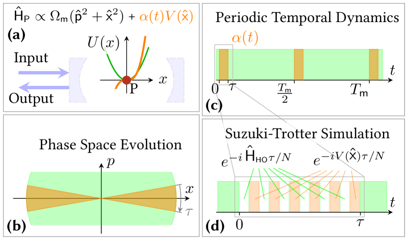
Figure 1: Scheme of the proposed stroboscopic method. (a) A levitated optomechanical system as an illustration of mechanical oscillator in a nonlinear potential. A dielectric subwavelength particle (P) is trapped by a tweezer (not shown). The particle feels a total potential $U(x)=\Omega_{\mathsf{m}}x^{2}/4+\alpha(t)V(x)$ that is a sum of the quadratic (green) and the nonlinear (orange, here: cubic) parts, both provided by the trapping beam. The particle can be placed inside a high-$Q$ cavity and probed by the laser light. (b,c) Stroboscopic application of nonlinear potential. The nonlinear part of the potential is switched on for only a short fraction of the mechanical period (orange segments). The quadratic trapping potential (green segments) is present throughout all the evolution. (d) Suzuki-Trotter simulation of stroboscopic evolution of the mechanical mode. In the figure, orange segments represent action of the nonlinear potential, empty and filled green segments correspond, respectively to unitary and damped harmonic evolution.

2.1 The nonlinear stroboscopic protocol

To implement the stroboscopic method, it is possible to versatilely use a levitated nanoparticle [45] with optical [6], electric [7] or magnetic [8] trapping. It is also possible to use a mirror equipped with a fully-optical spring [55], or a membrane with electrodes allowing its nonlinear actuation and driving [56]. In any of such systems, the mechanical mode can be posed into nonlinear potential $V(x)$, particularly, the cubic potential $V_{3}(x)\propto x^{3}$ for the pioneering test. In this manuscript we focus on the experimental parameters peculiar to the levitated nanoparticles [36, 37], although the principal results remain valid for the other systems as well. We also focus here solely on the evolution of the mechanical mode of the optomechanical cavity, assuming that the coupling to the optical cavity mode (blue in Fig. 1) is switched off.

The mechanical mode is a harmonic oscillator of eigenfrequency $\Omega_{\mathsf{m}}$, described by position and momentum quadratures, respectively, $\hat{x}$ and $\hat{p}$, normalized such that $\left[\hat{x},\hat{p}\right]=2\mathrm{i}$. The oscillator is coupled to a thermal bath at rate $\eta_{\mathsf{m}}$. We also assume fast stroboscopic application of an external nonlinear potential $\alpha(t)V(x)$ with a piecewise constant $\alpha(t)$ illustrating the possibility to periodically switch the nonlinear potential on and off as depicted at Fig. 1(a). The Hamiltonian of the system, therefore, reads ($\hbar=1$)

$$\hat{H}=\hat{H}_{\mathsf{HO}}+\alpha(t)V(\hat{x}),\quad\hat{H}_{\mathsf{HO}}=\frac{1}{4}\Omega_{\mathsf{m}}(\hat{x}^{2}+\hat{p}^{2}),$$ (1)

To illustrate the key idea behind the stroboscopic method, we first examine the regime of absent mechanical damping and decoherence. In this case, the unitary evolution of the oscillator is given by $\rho(t)=\hat{U}(t,t_{0})\rho(t_{0})\hat{U}^{\dagger}(t,t_{0})$, with $\hat{U}(t+\delta t,t)=\exp[-\mathrm{i}\hat{H}\delta t]$. When the nonlinearity is switched on permanently ($\alpha(t)=\alpha_{0}$), the free evolution dictated by $H_{\mathsf{HO}}$ mixes the quadratures of the oscillator which prohibits the resulting state from possessing properties of the target nonlinear quantum state arising purely from $V(x)$ regardless of the nonlinearity strength (see Supplementary Note 4 for more details). Willing to obtain a unitary transformation as close to $\exp[-\mathrm{i}V(\hat{x})\tau]$ as possible despite a constant presence of $\hat{H}_{\mathsf{HO}}$, we assume that the nonlinearity is repeatedly switched on for infinitesimally short intervals of duration $\tau$. If the duration $\tau$ is sufficiently short for the harmonic evolution to be negligible, the resulting evolution during $\tau$ is approximately purely caused by the $V(x)$ part of the Hamiltonian. To enhance the magnitude of the effect of the nonlinear potential, $V(\hat{x})$ we can apply it every $2\pi/\Omega_{\mathsf{m}}$ for short enough intervals as shown in Fig. 1 (b,c). This allows to establish an effective rotating frame within which the nonlinearity is protected from the effect of harmonic evolution. Realistically, the stroboscopic application corresponds to $\alpha(t)=\sum_{k}\delta_{\tau}(t-2\pi k/\Omega_{\mathsf{m}}),$ with $k\in\mathbb{Z}$, where $\delta_{\tau}$ is a physical approximation of Dirac delta function with width $\tau$ much shorter than the period of mechanical oscillations: $\tau\Omega_{\mathsf{m}}\ll 1$. Then we can consider the evolution over a number $M$ of harmonic oscillations as consisting of subsequent either purely harmonic or purely nonlinear steps, and the evolution operator can be approximately written as

$$\hat{U}(t+MT_{\mathsf{m}},t)=\left[\hat{U}(t+T_{\mathsf{m}},t)\right]^{M}\approx\left\{\exp[-\mathrm{i}\hat{H}_{\mathsf{HO}}T_{\mathsf{m}}]\exp[-\mathrm{i}V(\hat{x})\tau]\right\}^{M}=\exp[-\mathrm{i}MV(\hat{x})\tau].$$ (2)

For the last equality we used the fact that the unitary harmonic evolution through a single period of oscillations is an identity map: $\hat{U}_{\mathsf{HO}}(t+T_{\mathsf{m}},t)\equiv\exp[-\mathrm{i}\hat{H}_{\mathsf{HO}}T_{\mathsf{m}}]~{}=~{}\hat{\mathds{1}}$. Motion of a real mechanical oscillator can be approximated by a harmonic unitary evolution with good precision because of very high quality of mechanical modes of optomechanical systems [57, 35, 36]. Eq. 2 shows that the effect of sufficiently short pulses of the strong nonlinear potential timed to be turned on precisely once per a period of mechanical oscillations $M$ times, is equivalent to an $M$-fold increase of the nonlinearity.

A further improvement is possible by noting that undamped harmonic evolution over a half period simply flips the sign of the two quadratures $(\hat{x},\hat{p})\mapsto-(\hat{x},\hat{p})$. Therefore, it is possible to similarly apply the potential twice per period, switching its sign each second time. This can be formalized as setting $\alpha(t)=\sum_{k}(-1)^{k}\delta_{\tau}(t-\pi k/\Omega_{\mathsf{m}}),\ k~{}\in~{}\mathbb{Z}$. In this case,

$$\hat{U}(t+T_{\mathsf{m}},t)=\mathrm{e}^{-\mathrm{i}\hat{H}_{\mathsf{HO}}T_{\mathsf{m}}/2}\mathrm{e}^{+\mathrm{i}V(\hat{x})\tau}\mathrm{e}^{-\mathrm{i}\hat{H}_{\mathsf{HO}}T_{\mathsf{m}}/2}\mathrm{e}^{-\mathrm{i}V(\hat{x})\tau}=\mathrm{e}^{-2\mathrm{i}V(\hat{x})\tau},$$ (3)

and therefore, after $M$ periods

$$\hat{U}(t+MT_{\mathsf{m}},t)=\exp[-\mathrm{i}\cdot 2M\cdot V(\hat{x})\tau].$$ (4)

The idealised scheme proposed above in reality faces two potentially deteriorative factors: the finiteness of the duration of the nonlinearity $\tau$, and the mechanical decoherence caused by the thermal environment. We take a proper account of these two factors by considering the evolution as consisting of two kinds: (i) unitary undamped dynamics in a sum of the quadratic and nonlinear potentials, (ii) damped harmonic evolution between those. These two kinds of evolution are subsequently repeated, as shown in Fig. 1 (b,c). We develop an advanced method based on Suzuki-Trotter simulation (STS) to simulate the quantum state of a realistic optomechanical system after the application of our proposed protocol. It is worth noting that the STS is typically used to approximately achieve a novel evolution $\hat{U}$ from experimentally available exact unitaries [58, 59]. In our work, we use STS to simulate and justify that the experimentally available compound evolution $\hat{U}$ can approximate one of its building blocks $\hat{U}_{\mathsf{NL}}(\delta t)\equiv\exp(-\mathrm{i}V(x)\delta t)$. To verify the convergence of STS we also perform simulations in the Fock-state basis that allow direct computation of the propagator corresponding to the Hamiltonian (1). Fock-state-basis simulations unfortunately do not grant access to phase-space distributions such as Wigner function [60] which makes use of STS the primary strategy. Excellent agreement between the very distinct methods (STS and Fock-state-basis simulations) indicates that our results are correct. The details of the simulation methods are presented in Supplementary Notes 1 and 2.

We omit damping and thermal decoherence during the fast unitary action of the combined potential. Such applications are assumed to happen every half of a mechanical oscillation and have durations much shorter than the mechanical period, therefore, due to high quality of state-of-the-art mechanical oscillators, such omission is justified. The joint action is simulated using STS and verified by Fock-state-basis simulation. Between the applications of the nonlinear potential $V(x)$ the mechanical oscillator experiences damped harmonic evolution described by the linear Heisenberg-Langevin equations

$$\dot{x}=\Omega_{\mathsf{m}}p;\quad\dot{p}=-\Omega_{\mathsf{m}}x-\eta_{\mathsf{m}}p+\sqrt{2\eta_{\mathsf{m}}}\xi,$$ (5)

where $\xi$ is the quantum Langevin force, obeying $\left[\xi(t),x(t)\right]=\mathrm{i}\sqrt{2\eta_{\mathsf{m}}}$ and $\frac{1}{2}\left\langle\left\{\xi(t),\xi(t^{\prime})\right\}\right\rangle=(2n_{\mathsf{th}}+1)\delta(t-t^{\prime})$ with $n_{\mathsf{th}}$ being the mean occupation of the bath. The experimentally accessible value of the heating rate $H_{\mathsf{m}}$ is given by $H_{\mathsf{m}}=\eta_{\mathsf{m}}n_{\mathsf{th}}$. The density matrix $\rho(T_{\mathsf{m}}/2)$ of the particle after half of a period of oscillations including the action of the nonlinear potential and subsequent damping can be formally written as

$$\rho(\tau)=\mathcal{N}\left[\rho(0)\right]=\mathcal{D}\left[\hat{U}(\tau,0)\rho(0)\hat{U}^{\dagger}(\tau,0)\right].$$ (6)

where $\hat{U}(\tau,0)$ describes the particle’s unitary dynamics in combined potential, and $\mathcal{D}[\ \bullet\ ]$ indicates the mapping performed by the damping. Generalization of (6) to include the second half of the period, and the subsequent generalization to multiple periods, is straightforward.

Using these advanced numerical tools, further elaborated in Section 4 we evaluate the quantum state of the mechanical oscillator after the protocol and explore the limits of the achievable nonlinearities in the optomechanical systems that are accessible now or are within reach.

2.2 Application to the cubic nonlinearity

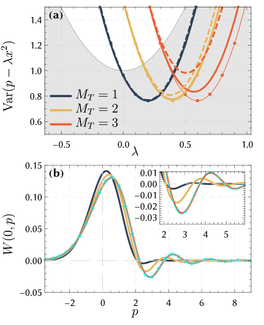
Figure 2: Results of the simulations. Results of stroboscopic application of cubic nonlinear potential $V=\gamma x^{3}/(6\tau)$ to the squeezed thermal state (initial occupation $n_{0}=0.05$, squeezing $s=1.2$) over multiple ($M_{\mathsf{T}}=1,2$ or $3$) halves of mechanical periods. (a) Squeezing of nonlinear quadrature. Thick lines correspond to stroboscopic method with realistic parameters and thermal noise, thin lines, to purely unitary application of the nonlinearity. Dashed lines correspond to the result of evolution driven by the full Hamiltonian $\hat{H}$ (1) from the same initial state over time $\tau,2\tau$ and $3\tau$ respectively. (b) Wigner function of motional states. Solid lines correspond to the same states from (a). Cyan line with markers (overlapping with solid red line) shows the unitary application of nonlinearity. Other parameters are: potential stiffness $\gamma=\gamma_{0}=0.2$, application duration $\tau\Omega_{\mathsf{m}}=\Theta=\Theta_{0}=\pi/100$, environmental thermal heating rate parameter $H_{0}=4\pi H_{\mathsf{m}}/\Omega_{\mathsf{m}}=0.002$.

Motivated by the role of cubic nonlinearity for the universal continuous-variable quantum processing, we illustrate the devised method by numerically evaluating the evolution of a levitated particle under a stroboscopic application of a cubic potential $V(x)\propto x^{3}$. The nonlinear phase gate $\mathrm{e}^{-\mathrm{i}V(x)}$ is a limit case of motion, it modifies only momentum of the object without any change of its position. This nondemolition aspect is crucial for use in universal quantum processing. A nonlinear phase state (particularly, the cubic phase state introduced in [3]) as the outcome of evolution of the momentum eigenstate $\left|p=0\right\rangle$ in a nonlinear potential $V(x)$ is defined as

$$\left|\gamma_{V}\right\rangle\propto\int\mathrm{d}x\>\mathrm{e}^{\mathrm{i}V(x)\tau}\left|x\right\rangle,$$ (7)

where $V(x)$, is a highly nonlinear potential, and $\left|x\right\rangle$ the position eigenstate $\hat{x}\left|x\right\rangle=x$. The state (7) requires an infinite squeezing possessed by the ideal momentum eigenstate before the nonlinear potential is applied. More physical is an approximation of this state obtained from a finitely squeezed thermal state $\rho_{0}(r,n_{0})$, ideally, vacuum, by the application of $V$:

$$\rho(V,r,n_{0})=\mathrm{e}^{\mathrm{i}V(\hat{x})\tau}\rho_{0}(r,n_{0})\mathrm{e}^{-\mathrm{i}V(\hat{x})\tau}.$$ (8)

The initial state $\rho_{0}$ is the result of squeezing a thermal state with initial occupation $n_{0}$

$$\rho_{0}(r,n_{0})=\hat{S}(r)\rho_{0}(0,n_{0})\hat{S}^{\dagger}(r)$$ (9)

where $\hat{S}(r)=\exp[\tfrac{1}{2}r^{*}(\hat{a})^{2}-\tfrac{1}{2}r(\hat{a}^{\dagger})^{2}]$ is a squeezing operator ($\hat{a}=(\hat{x}+\mathrm{i}\hat{p})/2$), and the initial state $\rho_{0}$ is thermal with mean occupation $n_{0}$. Phase of the squeezing parameter $r=|r|\mathrm{e}^{\mathrm{i}\theta}$ determines the squeezing direction. When $n_{0}=0$, $|r|\to+\infty$, and $\theta=\pi$, the initial state is infinitely squeezed in $p$, and  Eq. 8 approaches the ideal cubic state (7).

The quantum state obtained as a result of the considered sequence of interactions approximates the ideal state given by Eq. 7. The quality of the approximation can be assessed by evaluating the variance of a nonlinear quadrature $p-\lambda x^{2}$, or the cuts of the Wigner functions of the states. A reduction in nonlinear quadrature variance below the vacuum is a necessary condition for application of these states in nonlinear circuits [51, 52]. On the other hand, the phase-space interference fringes of the Wigner function reaching negative values are a very sensitive witness of quantum non-Gaussianity of the states used in the recent experiments [61, 62, 63, 64]. Fidelity happens to be an improper measure of the success of the preparation of the quantum resource state [65] because it does not predict either applicability of these states as resources or their highly nonclassical aspects.

A noise reduction in the cubic phase gate can be a relevant first experimental test of the quality of our method. The approximate cubic state obtained from a squeezed thermal state (that is, the state (8) with $V(x)=\gamma x^{3}/(6\tau)$) should possess arbitrary high squeezing in the variable $p-\lambda x^{2}$ for $n_{0}=0$ given sufficient squeezing of the initial mechanical state. The state (8) obtained from a squeezed in momentum state, has the following variance of the nonlinear quadrature

$$\sigma_{3}^{\rho}(\lambda)\equiv\operatorname*{\operatorname{Tr}}(\rho(\hat{p}-\lambda\hat{x}^{2})^{2})-\left(\operatorname*{\operatorname{Tr}}\rho(\hat{p}-\lambda\hat{x}^{2})\right)^{2}=\frac{v_{\mathsf{th}}}{s^{2}}+2(\lambda-\gamma)^{2}(s^{2}v_{\mathsf{th}})^{2},$$ (10)

where $v_{\mathsf{th}}=2n_{0}+1$ is the variance of each canonical quadrature in the initial thermal state before squeezing, and $s=\mathrm{e}^{r}$ is the magnitude of squeezing. An important threshold is the variance of the nonlinear quadrature attained at the vacuum state ($n_{0}=0$, $s=1$)

$$\sigma_{3}^{\text{vac}}(\lambda)=1+2\lambda^{2}.$$ (11)

Application of a unitary cubic evolution to the initial vacuum state displaces this curve along the $\lambda$ axis by $\gamma$. Further, as follows from Eq. 10, squeezing the initial state allows reducing the minimal value of $\sigma_{3}$, and increase of the initial occupation $n_{0}$ causes also increase of $\sigma_{3}$. Suppression of fluctuations in the nonlinear quadrature is a convenient figure of merit because it is a direct witness of the applicability of the quantum state as a resource for measurement-based quantum information processing [51, 52] and a witness of non-classicallity [66]. It can be evaluated in an optomechanical systems with feasible parameters using pulsed optomechanical interaction [66] without a full quantum state tomography.

In Fig. 2 (a) we show the variance $\sigma_{3}$ at the instants $t=M_{\mathsf{T}}T_{\mathsf{m}}/2$. Each of the curves takes into account also the interaction with the thermal environment lasting $T_{\mathsf{m}}/2$ after each application of the nonlinearity. The heating rate parameter $H_{0}=4\pi H_{\mathsf{m}}/\Omega_{\mathsf{m}}$ assumes value $H_{0}=2\times 10^{-3}$. For an oscillator of eigenfrequency $\Omega_{\mathsf{m}}=2\pi\times$100\text{\,}\mathrm{kHz}$$ and $Q=10^{6}$ is equivalent to occupation of the environment equal to $n_{\mathsf{th}}\approx 10^{7}$ phonons. This is the equilibrium occupation of such an oscillator at the temperature of $50\text{\,}\mathrm{K}$. A recent experiment of ground state cooling of a levitated nanoparticle [37] reported the heating rate corresponding to $H\approx 10^{2}H_{0}$. A proof of robustness of the method against such heating is in the Supplementary Note 3.

Thin lines with markers show the analytic curves defined by Eq. 10 for the corresponding values of $\gamma$. The good quantitative correspondence between the approximate states resulting from the realistic stroboscopic application of nonlinear potential and the analytic curves again proves the validity of the stroboscopic method. Importantly, each of the curves has an area where it lies below the corresponding ground-state level $\sigma_{3}^{\text{vac}}$. This means each of the corresponding states gives advantage over vacuum if used as ancilla for the cubic gate. The dashed lines show the simulated quantum states obtained from the same initial state by longer unitary evolution according to the full Hamiltonian from Eq. 1, that is $\mathrm{e}^{-\mathrm{i}\hat{H}n\tau}\rho\mathrm{e}^{\mathrm{i}\hat{H}n\tau}$ where $n=1,2,3$ for blue, yellow and red correspondingly. Further divergence from ideal than that of the ones corresponding to the stroboscopic method witnesses an advantage of the latter in generation of the resource for the measurement-based computation.

The stroboscopic application of a fixed limited gain nonlinearity, therefore, indeed allows amplification of nonlinearity in accordance with Eq. 4. Importantly, even despite requiring longer evolution in a noisy environment, the stroboscopic method allows better amplification than a unitary longer application of the nonlinearity in presence of the free evolution ($\propto\hat{p}^{2}$) and harmonic ($\propto\hat{x}^{2}$) terms in the Hamiltonian.

The non-Gaussian character of the prepared quantum state can be witnessed via its Wigner function $W(x,p)$ which for a quantum state $\rho$ reads [67]

$$W(x,p)=\frac{1}{2\pi}\int\limits_{-\infty}^{\infty}\mathrm{d}y\>\mathrm{e}^{-\mathrm{i}py}\left\langle x+y\middle|\rho\middle|x-y\right\rangle.$$ (12)

Wigner function (WF) shows a quasiprobability distribution over the phase space spanned by position $x$ and momentum $p$ and its negativity is a prerequisite of the non-classicallity of a quantum state. In Fig. 2 (b) are Wigner functions $W(0,p)$ of the mechanical oscillator computed for the same approximate states as in the panel (a). The Wigner function of an ideal cubic phase state, i.e. the state given by Eq. 7 for $V(x)=x^{3}\gamma/(6\tau)$, reads [3, 50]

$$W_{\mathsf{CPS}}(x,p)\propto\operatorname*{Ai}\left[\left(\frac{4}{\gamma}\right)^{1/3}\left(\gamma x^{2}-p\right)\right],$$ (13)

where $\operatorname*{Ai}(x)$ is the Airy function. This function with apparent non-Gaussian shape in the phase space exhibits fast oscillations reaching negative values in the positive momentum for any $\gamma>0$. The Wigner functions of the states obtained by application of the stroboscopic protocol approach the one of Eq. 8. Each of them exhibits areas with negative values which proves quantum non-Gaussian character of the resulting state. Moreover, with increased number of stroboscopic applications involved, the resulting approximate state corresponds to stronger nonlinearity. For the last curve where $M_{\mathsf{T}}=3$ we also show the result of an idealized instantaneous unitary application of an equal total nonlinearity by a cyan line with markers which is indistinguishable from the line for the approximate evolution. For this pair of curves we also have an estimate for the overlap $\operatorname*{\operatorname{Tr}}[\rho_{\mathsf{red}}\rho_{\mathsf{cyan}}]/\operatorname*{\operatorname{Tr}}[\rho_{\mathsf{cyan}}^{2}]=0.9877$. Despite an excellent overlap of the ideal and approximate Wigner functions, the important resource, squeezing $\sigma_{3}$ shows a noticeable deviation from the ideal scenario. It is for this reason that we choose the squeezing $\sigma_{3}$ as the main figure of merit for the protocol.

3 Discussion

In this article we have proposed and theoretically analyzed a protocol to create a nonlinear motional state of the mechanical mode of an optomechanical system with controllable nonlinear mechanical potential. The method uses the possibility to apply the nonlinear potential to the motion of mechanical object in a stroboscopic way, twice per a period of oscillations. This way of application allows reducing the deteriorative effect of the free oscillations and approach the effect of pure action of nonlinear potential. In contrast to other methods of creating non-classical states by a continuous evolution in presence of nonlinear terms in the Hamiltonian [68, 69, 70], our method allows approaching the states that approximate evolution according to the unitary $\mathrm{e}^{\mathrm{i}V(x)}$ where $V(x)$ is the nonlinear potential profile. We tested our method on a cubic nonlinearity $\propto\hat{x}^{3}$ though the method is applicable to a wide variety of nonlinearities. Our simulations prove that application of the protocol allows one to obtain the squeezing in the nonlinear quadrature below the shot-noise level even if the initial state of the particle is not pure. The nonlinear state created in a stroboscopic protocol clearly outperforms as a resource the vacuum for which the bound (11) holds. Moreover, the stroboscopic states approximate the one defined by Eq. 8 obtained in absence of the free rotation and thermal decoherence. We also verify that the stroboscopic application of the cubic nonlinear potential generates nonclassical states under conditions that are further from optimal than the ones of Fig. 2. In particular, we find that the heating rate $H_{\mathsf{m}}$ can be increased approximately 100-fold until the curve $\sigma_{3}(\lambda)$ fails to overcome the vacuum boundary $1+2\lambda^{2}$. We are able to prove that when the duration of the application $\tau$ is increased tenfold such that the corresponding product $V(x)\tau$ remains constant, (that is, a less stiff potential is applied stroboscopically for proportionally longer time intervals), the resulting nonlinear state as well shows squeezing in $\sigma_{3}$. This proves robustness of the method to the two major imperfections.

We have shown the method to work for the parameters inspired by recent results demonstrated by the levitated optomechanical systems [71, 72]. The optical trap with a cubic potential has been already used in the experiments [43, 44]. Levitated systems [22], including electromechanical systems [73], have recently shown significant progress in the motional state cooling [35, 36, 37] and feedback-enhanced operation [34] which lays solid groundwork of the success of the proposed protocol. The authors of Ref. [44] report the experimental realisation of the potential $V(X)=\mu X^{3}/6$ with $\mu\approx 8k_{\mathsf{B}}T$\text{\,}\mathrm{\SIUnitSymbolMicro}\mathrm{m}^{-3}$$, where $X=x\sqrt{\hbar/(2m\Omega_{\mathsf{m}})}$ is the dimensional displacement of the oscillator, $m$ is its mass, $k_{\mathsf{B}}$ is the Boltzmann constant and $T$ temperature. From this value we can make a very approximate estimate for the nonlinear gain $\gamma=\mu(\hbar/(2m\Omega_{\mathsf{m}}))^{3/2}\tau\approx 1.2\times 10^{-3}$ assuming duration $\tau=\pi/(50\Omega_{\mathsf{m}})$, temperature $T=$300\text{\,}\mathrm{K}$$, frequency $\Omega_{\mathsf{m}}=2\pi\times$1\text{\,}\mathrm{kHz}$$, and a mass $m=$4\text{\times}{10}^{-15}\text{\,}\mathrm{g}$$ of a silica nanoparticle of $70\text{\,}\mathrm{nm}$ radius.

Experimental implementation of the proposed method can guarantee preparation of a strongly nongaussian quantum motional state. Further analysis of such a state will require either a full state tomography or better suited well-tailored methods to prove the nonclassicality [74]. An analysis of the estimation of the non-linear mechanical quadrature variance via pulsed optomechanical interaction can be found in [66]. The optical read out can be improved using squeezed states of light [75]. This experimental step will open applications of the proposed method to other nonlinear potentials relevant for quantum computation [4, 76, 51, 52], quantum thermodynamics [77, 78] and quantum force sensing [79, 80].

In our simulations we focused solely on the dynamics of the mechanical mode and assumed the conventional optomechanical interaction absent. This interaction, well developed in recent years, provides a sufficiently rich toolbox that allows incorporation of the mechanical mode into the optical circuits of choice [9]. As an option, a prepared nonlinear state can be transferred to traveling light pulse [75] using optomechanical driving. In a more complicated scenario, one can add optomechanical interaction to the stroboscopic evolution to obtain even richer dynamics. A complete investigation of such dynamics, however, goes beyond the scope of the present research focused on the preparation of nonlinear motional states.

In parallel with the experimental verification, the stroboscopic method can be used to analyse other higher-order mechanical nonlinearities such as $V(x)\propto x^{4}$ or tilted double-well potentials required for tests of recently disputed quantum Landauer principle [81], counter-intuitive Fock state preparation [82] and approaching macroscopic superpositions [83].

4 Methods

4.1 Tools of numerical simulations

The Eq. 6 approximates the damped evolution of an oscillator in a nonlinear potential by a sequence of individual stages of harmonic, nonlinear and damped harmonic evolution (see Fig. 1). Below we elaborate on how it is possible to simulate such dynamics using Wigner function in the phase space, density matrix in position, momentum and Fock basis.

First, we evaluate the action of the nonlinearity during the stroboscopic pulse. While the nonlinearity is on, the Hamiltonian of the system reads

$$\hat{H}=\hat{H}_{\mathsf{HO}}+V(\hat{x})=\hat{H}_{p}+\hat{H}_{x},$$ (14)

where $\hat{H}_{p}=\frac{\Omega_{\mathsf{m}}}{4}\hat{p}^{2},$ and $\hat{H}_{x}=\frac{\Omega_{\mathsf{m}}}{4}\hat{x}^{2}+\frac{\gamma}{6}\hat{x}^{3}.$

Our important simulation tool is the Suzuki-Trotter simulation (STS, see Ref. [48]) for $\hat{U}$

$$\hat{U}(t+\tau,t)=\Big{[}\exp[-\mathrm{i}(\hat{H}_{\mathsf{HO}}+V(\hat{x}))\tfrac{\tau}{N}]\Big{]}^{N}=\Big{[}\hat{U}_{\mathsf{HO}}(\tfrac{\tau}{N})\hat{U}_{\mathsf{NL}}(\tfrac{\tau}{N})+O\left(\left(\tfrac{\tau}{N}\right)^{2}\right)\Big{]}^{N},$$ (15)

where $\hat{U}_{\mathsf{HO}}(\delta t)\equiv\exp(-\mathrm{i}H_{\mathsf{HO}}\delta t)$, $\hat{U}_{\mathsf{NL}}(\delta t)\equiv\exp(-\mathrm{i}V(x)\delta t)$, $N$ is called the Trotter number. The accuracy of the approximation is, thereby, increasing with decreasing $\tau/N$. Despite $\tau$ being now sufficiently large to take into account noticeable free rotation through an angle $\Omega_{\mathsf{m}}\tau$ in the phase space, we still assume that $\tau$ is much shorter than the mechanical decoherence timescale, set by the heating rate $H_{\mathsf{m}}$. This is well justified for the current experiments [33, 36, 37], also see Supplementary Note 2. The STS requires the summands forming the Hamiltonian to be self-adjoint which is not always the case of $V(x)$, in particular $V(x)\propto x^{3}$. We take the necessary precautions by considering such nonlinearities over only short time in a finite region of the phase space. Thus we cautiously take care of the quantum motional state being limited to this finite region. To further verify the correctness of numerics via STS, we cross-check it using numerical simulations in Fock-state basis.

Eq. 14 shows the two possibilities to split the full Hamiltonian into summands to use the STS. We use these two possibilities to compute independently the mechanical state in order to verify the correctness of the STS in Supplementary Note 1.

First, we start from a squeezed thermal state $\rho(0)$, which has a representation by the Wigner function in the phase space

$$W_{\mathsf{th}}(x,p;n_{0},s)=\frac{\exp\left(-\frac{1}{2}\left[\frac{(x/s)^{2}+(ps)^{2}}{2n_{0}+1}\right]\right)}{2\pi(2n_{0}+1)}.$$ (16)

The Wigner function corresponding to a quantum state $\rho$ is defined [67] as

$$W(x,p)=\frac{1}{2\pi}\int\limits_{-\infty}^{\infty}\mathrm{d}y\>\mathrm{e}^{-\mathrm{i}py}\left\langle x+y\middle|\rho\middle|x-y\right\rangle,$$ (17)

and the corresponding density matrix element can be obtained from the Wigner function by an inverse Fourier transform. It is therefore possible to extend this approach to any $W(x,p)$ beyond the Gaussian states.

The evolution of a state $\rho$ under action of a Hamiltonian proportional to a quadrature $\hat{q}$ can be straightforwardly computed in the basis of this quadrature, where it amounts to multiplication of density matrix elements with $c$-numbers:

$$\left\langle q\right|\mathrm{e}^{-\mathrm{i}\hat{H}_{q}(\hat{q})t}\rho\mathrm{e}^{\mathrm{i}\hat{H}_{q}(\hat{q})t}\left|q^{\prime}\right\rangle=\left\langle q\middle|\rho\middle|q^{\prime}\right\rangle\mathrm{e}^{-\mathrm{i}(H_{q}(q)-H_{q^{\prime}}(q^{\prime}))t}.$$ (18)

In particular, the nonlinear evolution reads

$$\left\langle x\right|\hat{U}_{\mathsf{NL}}(\delta t)\rho\hat{U}^{\dagger}_{\mathsf{NL}}(\delta t)\left|x^{\prime}\right\rangle=\left\langle x\right|\rho\left|x^{\prime}\right\rangle\mathrm{e}^{-\mathrm{i}[V(x)-V(x^{\prime})]\delta t}.$$ (19)

The undamped harmonic evolution driven by $\hat{H}_{\mathsf{HO}}$ can be represented by the rotation of Wigner function (WF) in the phase space. A unitary rotation through an angle $\theta=\Omega_{\mathsf{m}}\delta t$ in the phase space maps the initial WF $W(x,p;t)$ onto the final $W(x,p;t+\delta t)$ as

$$W(x,p;t+\delta t)=W(x\cos\theta-p\sin\theta,p\cos\theta+x\sin\theta;t).$$ (20)

The unitary transformation of the density matrix can be as well computed in the Fock state basis.

Finally, damped harmonic evolution of a high-Q harmonic oscillator over one half of an oscillation can also be evaluated in the phase space as a convolution of the initial Wigner function $W(x,p;t)$ with a thermal kernel

$$W(x,p;t+\frac{\pi}{\Omega})=\iint\limits_{-\infty}^{\infty}\mathrm{d}u\>\mathrm{d}v\>W_{i}(x-u,p-v;t)W_{\mathsf{B}}(u,v),$$ (21)

where the expression for the kernel reads

$$W_{\mathsf{B}}(u,v)=\frac{1}{2\pi\sigma_{\mathsf{th}}}\exp\left[-\frac{u^{2}+v^{2}}{2\sigma_{\mathsf{th}}}\right],$$ (22)

with $\sigma_{\mathsf{th}}=(2n_{\mathsf{th}}+1){2\pi\eta_{\mathsf{m}}}/{\Omega_{\mathsf{m}}}$, where $n_{\mathsf{th}}\approx k_{\mathsf{B}}T/(\hbar\Omega_{\mathsf{m}})$ is the thermal occupation of the bath set by its temperature $T$. In terms of the heating rate $H_{\mathsf{m}}$, $\sigma_{\mathsf{th}}=4\pi H_{\mathsf{m}}/\Omega_{\mathsf{m}}$. Eq. 21 is obtained by solving the joint dynamics of the oscillator and bath followed by tracing out the latter. The detailed derivation of Eq. 21 can be found in Supplementary Note 2.

Using these techniques, one can evaluate the action of the map $\mathcal{N}$ defined by Eq. 6 on the state of the quantum oscillator. This yields the quantum state of the particle after one half of a mechanical oscillation. Repeatedly applying the same operations, one can obtain the state after multiple periods of the mechanical oscillations. Our purpose is then to explore the limits of the achievable nonlinearities in optomechanical systems that are accessible now or are within reach.

Data Availability

The datasets generated and analyzed during the current study are available from the corresponding author on reasonable request.

Author Contributions

R.F. conceived the theoretical idea. A.A.R. performed the numerical computations. Both authors participated in writing the manuscript.

Competing Interests

The authors declare no competing interests.

Supplementary Information: Stroboscopic high-order nonlinearity for quantum optomechanics

Supplementary Note 5-4 Convergence of the Suzuki-Trotter approximation

In this section we numerically demonstrate that the Suzuki-Trotter approximation that we use to simulate the combined dynamics, indeed converges. For this purpose we provide the plots of the variance of nonlinear variable $\operatorname*{\operatorname{Var}}(p-\lambda x^{2})$ computed in the approximate nonlinear state

$$\rho(\tau)=\hat{U}(\tau,0)\rho(0)\hat{U}^{\dagger}(\tau,0),$$ (S23-22)

where $\hat{U}(\tau,0)=\exp[-\mathrm{i}\hat{H}\tau]$ using different methods.

For the first two, we use the Suzuki-Trotter expansion of the unitary operator $\hat{U}$

$$\exp[-\mathrm{i}(\hat{H}_{1}+\hat{H}_{2})N\delta\tau]\approx\left(\exp[-\mathrm{i}\hat{H}_{1}\delta\tau]\times\exp[-\mathrm{i}\hat{H}_{2}\delta\tau]\right)^{N},$$ (S24-22)

where, depending on the method, we choose either

$$\text{Method 1:}\quad\hat{H}_{1}=\hat{H}_{p},\quad\hat{H}_{2}=\hat{H}_{x},$$ (S25-22)

or

$$\text{Method 2:}\quad\hat{H}_{1}=\hat{H}_{\mathsf{HO}},\quad\hat{H}_{2}=V(\hat{x}),$$ (S26-22)

with notations of Eq. 14. The action of individual unitary operators in Method 1 is computed in the corresponding quadrature basis according to Eq. 18. In Method 2 the action of $\hat{H}_{1}$ is simulated by rotation of the Wigner function in the phase space according to Eq. 20, and the action of $\hat{H}_{2}$ in the position basis as in Eq. 18. In the main text, Method 1 is used to produce the results.

For the Method 3, we write the Hamiltonian $\hat{H}$ in the Fock state basis. This allows to directly compute matrix elements of $\hat{U}(\tau,0)$ in the Fock basis as well, without the need to use STS, and directly obtain the approximate nonlinear state. This method, unfortunately, does not allow to obtain Wigner function directly.

Comparison of the nonlinear variances from different methods is in Supplementary Fig. S3-2. We show that as the Trotter number $N$ increases, the simulation using Method 1 converges. The similarly converging simulation using Method 2 is not shown to avoid cluttering of the figure. Both methods approximately converge to the simulations in the Fock basis. Method 2 shows larger deviation since the operation of rotation of the Wigner function in the phase space involves interpolation and is therefore less accurate. This is the reason to choose Method 1 for the main text. Good numerical coincidence of the results of all the three different methods proves convergence of the STS.

As an experiment, we also simulate the regime of operation that is accessible only to the levitated nanoparticles. In such systems, one has in principle full control over the potential that the particle is exposed to, and can, therefore alternate between the quadratic trapping potential and the higher-order nonlinear one. Formally this corresponds to having a Hamiltonian that, instead of Eq. 1, reads

$$\hat{H}=\frac{\Omega_{\mathsf{m}}}{4}\Big{[}\hat{p}^{2}+(1-\alpha(t))\hat{x}^{2}\Big{]}+\alpha(t)V(\hat{x}).$$ (S27-22)

We also simulate the action of the nonlinear stage of this Hamiltonian, that is the action of $\hat{H}=\Omega_{\mathsf{m}}\hat{p}^{2}/4+\gamma\hat{x}^{3}/6$, using Methods 1 and 3. That is we simulate this regime using STS and Fock-state expansion. The results of simulation show good agreement what again proves the STS convergence. The nonlinear quadrature is squeezed stronger in this regime, which suggests that the strategy to switch between the potentials can be advantageous for the levitated nanoparticles, or other systems where a full control over the potential is available.

Supplementary Note 6-4 Impact of the thermal noise

Owing to recent progress in design and manufacturing of the nanomechanical devices, the thermal noise is strongly suppressed. In this section we check the robustness of our scheme to the thermal noise from the environment and show that for the state-of-the art systems it is not hampering the quantum performance.

The thermal noise can be included by writing the standard Langevin equations:

$$\dot{x}=\Omega_{\mathsf{m}}p;\quad\dot{p}=-\Omega_{\mathsf{m}}x-\eta_{\mathsf{m}}p+\sqrt{2\eta_{\mathsf{m}}}\xi,$$ (S28-22)

where $\xi$ is the quantum Langevin force, obeying the commutation relation $\left[\xi(t),x(t)\right]=\mathrm{i}\sqrt{2\eta_{\mathsf{m}}}$ and markovian autocorrelation $\frac{1}{2}\left\langle\left\{\xi(t),\xi(t^{\prime})\right\}\right\rangle=2n_{\mathsf{th}}+1$.

The solution of these equations corresponding to one half of a period of the mechanical oscillations ($\tau_{\mathsf{m}}=\pi/\Omega_{\mathsf{m}}$) for the experimentally relevant regime of high-Q mechanical oscillator ($Q\equiv\Omega_{\mathsf{m}}/\eta_{\mathsf{m}}\gg 1$) reads

$$x^{\prime} =\mathrm{e}^{-\eta_{\mathsf{m}}\tau_{\mathsf{m}}/2}\Big{[}(\cos\zeta+\epsilon\sin\zeta)x(0)+\frac{1}{\sigma}\sin\zeta p(0)+\delta x(\tau_{\mathsf{m}})\Big{]},$$ (S29-22)

$$p^{\prime} =\mathrm{e}^{-\eta_{\mathsf{m}}\tau_{\mathsf{m}}/2}\Big{[}(\cos\zeta-\epsilon\sin\zeta)p(0)+\frac{1}{\sigma}\sin\zeta x(0)+\delta p(\tau_{\mathsf{m}})\Big{]},$$ (S30-22)

with $\zeta=\Omega_{\mathsf{m}}\tau_{\mathsf{m}}\sigma$, $\sigma=\sqrt{1-(\eta_{\mathsf{m}}/2\Omega_{\mathsf{m}})}$ and $\epsilon=\eta_{\mathsf{m}}/(2\Omega_{\mathsf{m}}\sigma)$. The definitions for the noise operators $\delta x,\delta p$ read

$$\delta x(\tau_{\mathsf{m}}) =\sqrt{2\eta_{\mathsf{m}}}\int_{0}^{\tau_{\mathsf{m}}}\mathrm{d}t\>\mathrm{e}^{\eta_{\mathsf{m}}t/2}\sin\Omega_{\mathsf{m}}\sigma(\tau_{\mathsf{m}}-t)\xi(t),$$ (S31-22)

$$\delta p(\tau_{\mathsf{m}}) =\sqrt{2\eta_{\mathsf{m}}}\int_{0}^{\tau_{\mathsf{m}}}\mathrm{d}t\>\mathrm{e}^{\eta_{\mathsf{m}}t/2}\Big{[}\cos\Omega_{\mathsf{m}}\sigma(\tau_{\mathsf{m}}-t)-\epsilon\sin\Omega_{\mathsf{m}}\sigma(\tau_{\mathsf{m}}-t)\Big{]}\xi(t).$$ (S32-22)

These are the canonical quadratures of a mode in a thermal state with variance $\sigma_{\mathsf{th}}=2n_{\mathsf{th}}+1$.

The transformation of the Wigner function can be found as follows. Consider that at instant $t=0$ the mechanical oscillator has WF $W_{\mathsf{m}}(x(0),p(0))$. The mode of the bath is in a thermal state with WF

$$W_{\mathsf{B}}(\delta x,\delta p;\sigma_{\mathsf{th}})=\frac{1}{2\pi\sigma_{\mathsf{th}}}\exp\left[-\frac{\delta x^{2}+\delta p^{2}}{2\sigma_{\mathsf{th}}}\right].$$ (S33-22)

Assuming the joint evolution of the mechanical oscillator and bath to be unitary, one can write the WF of the composite system (mechanical oscillator+bath)

$$W(x^{\prime},p^{\prime},\delta x,\delta p)=W_{\mathsf{m}}(x[x^{\prime},p^{\prime},\delta x,\delta p],p[x^{\prime},p^{\prime},\delta x,\delta p])\times W_{\mathsf{B}}(\delta x,\delta p).$$ (S34-22)

Here the first argument of $W_{\mathsf{m}}$, $x[\dots]$, means the solution of Eqs. S29-22 and S30-22 for $x$ etc. Since in the contemporary experiments the quality-factors of the mechanical oscillators can exceed $Q=10^{6}$ (see e.g. [57, 35, 36]), one can approximate $\sigma\approx 1$, $\epsilon=0$, $\zeta=\pi$ with accuracy $o(Q^{-1})$. Moreover, $\exp[-\eta_{\mathsf{m}}\tau_{\mathsf{m}}/2]\approx 1$. Therefore

$$x\approx x^{\prime}-\sqrt{\frac{2\pi\eta_{\mathsf{m}}}{\Omega_{\mathsf{m}}}}\delta x\equiv x^{\prime}-\theta\delta x,\quad p\approx p^{\prime}-\theta\delta p,\quad\theta\equiv\sqrt{\frac{2\pi\eta_{\mathsf{m}}}{\Omega_{\mathsf{m}}}}.$$ (S35-22)

To obtain the WF of the mechanical oscillator after this evolution, one has to trace out the degrees of freedom of the environment

$$W^{\prime}(x^{\prime},p^{\prime})=\iint\mathrm{d}(\>\delta x)\mathrm{d}(\>\delta p)W_{\mathsf{m}}(x^{\prime}-\theta\delta x,p^{\prime}-\theta\delta p)W_{\mathsf{B}}(\delta x,\delta p;\sigma_{\mathsf{th}}).$$ (S36-22)

Making a substitution $(u,v)=\theta\cdot(\delta x,\delta p)$ we arrive to the simple expression

$$W^{\prime}(x^{\prime},p^{\prime})=\iint\mathrm{d}u\>\mathrm{d}v\>W_{\mathsf{m}}(x^{\prime}-u,p^{\prime}-v)W^{\prime}_{\mathsf{B}}(u,v),$$ (S37-22)

where $W^{\prime}_{\mathsf{B}}(u,v)=W_{\mathsf{B}}(u,v,\sigma_{\mathsf{th}}\theta^{2})$. The Eq. S37-22 describes a convolution of the initial Wigner function $W_{\mathsf{m}}$ with a WF of a thermal state, whose variance is reduced by the mechanical $Q$-factor. Due to this rescaling, $W^{\prime}_{\mathsf{B}}$ is a very narrow Gaussian distribution, with variance much below $1$. In this manuscript we use primarily the value $\sigma_{\mathsf{th}}\theta^{2}=4\pi\frac{H_{\mathsf{m}}}{\Omega_{\mathsf{m}}}\equiv H_{0}=0.002$ which, for an oscillator of eigenfrequency $\Omega_{\mathsf{m}}=2\pi\times$100\text{\,}\mathrm{kHz}$$ and $Q=10^{6}$ is equivalent to occupation of the environment equal to $n_{\mathsf{th}}\approx 10^{7}$ phonons. This is the equilibrium occupation of such an oscillator at the temperature of $50\text{\,}\mathrm{K}$.

Supplementary Note 7-4 Robustness of the stroboscopic method

In this section, to prove the feasibility of the stroboscopic method, we evaluate the robustness of our method against the finiteness (non-instantaneousness) of the duration of the nonlinearity and the impact of the thermal noise. It is convenient to measure the temporal extent $\tau$ of the nonlinear potential application in units of the mechanical motion period $\Theta=\Omega_{\mathsf{m}}\tau$, so that $\Theta=2\pi$ corresponds to a full mechanical oscillation. In Supplementary Fig. S4-2 (a) we plot the variance of nonlinear quadrature as a function of the free parameter for different values of the phase rotation $\Theta$. The plots illustrate that as the phase gain $\Theta$ from the quadratic evolution decreases, the result of the combined dynamics approaches the action of the pure nonlinearity. In particular, for the value in the figure, difference in the minimal value of the nonlinear variance is less than 10%. As the strength of the applied nonlinear potential increases, the nonlinear squeezing becomes more sensitive to the free rotation. The reason is apparently because the state with stronger nonlinearity is further from the classical domain and hence more fragile to perturbations.

In Supplementary Fig. S4-2 (b) we show the nonlinear variance from Supplementary Fig. S4-2 for the value $\Theta=\pi/20$ after one half of mechanical period in the thermal environment. We can see that in the setup of the present experiment with levitated nanoparticles [37], for which $H=10^{2}H_{0}$ most of the nonlinear squeezing is lost, however for a narrow region of the parameter values the mechanical state can still be used as a resource of the nonlinear squeezing. In case of the heating rate being suppressed tenfold, the nonlinear squeezing persists in the thermal environment. It has to be noted that in electromechanical or optomechanical experiments with bulk oscillators, typical heating rates are much smaller. For instance, in electromechanical experiment [85], $H_{\mathsf{m}}=1.4\times 10^{-3}\Omega_{\mathsf{m}}$, and in the experiment with optomechanical crystal reported in Ref. [17], $H_{\mathsf{m}}<0.1\times 10^{-3}\Omega_{\mathsf{m}}$.

Supplementary Note 8-4 On duration of the nonlinear potential application

One possibility to use the nonlinear potential that seems straightforward, is to apply it simultaneously with the quadratic one and investigate the steady state. This strategy, unfortunately does not allow seeing coherent effects of nonlinearity. In this section we explore application of nonlinear potential for durations comparable to the mechanical period and show that the stroboscopic application is optimal.

First, we have to note that a mechanical oscillator in a sum of quadratic and an odd-order potentials will have a steady state only in the case of weak cubic nonlinearity when there exists a local minimum. Then the oscillator is going to be trapped in its vicinity where the effective potential is a displaced quadratic one. Therefore, we only have to consider finite-time action of the cubic potential and show that increasing the duration of nonlinear potential’s action decreases its effect.

The unitary dynamics of an oscillator in presence of both quadratic and polynomial potential is described by the operator which in our notations for the nonlinear gain $\gamma$ can be written as

$$\hat{U}(\tau)=\exp\left(-\mathrm{i}\left[\frac{\Omega}{4}(p^{2}+x^{2})+\frac{\gamma}{2k\tau}x^{k}\right]\tau\right).$$ (S38-22)

The resulting action of this unitary is determined by two parameters: total phase rotation $\Omega\tau$ and nonlinear gain $\gamma$. In the experiment, however, the parameters that are defined by the external control (e.g., optical driving) are the stiffnesses of quadratic and polynomial potentials, respectively, $\Omega$ and $\varkappa=\gamma/\tau$.

In this light, there are two different ways to compare longer interactions:

• Assuming constant stiffnesses but longer duration

  $$\hat{U}(\tau^{\prime})=\exp\left(-i\left[\frac{\Omega}{4}(p^{2}+x^{2})+\frac{\gamma}{2k\tau}x^{k}\right]\tau^{\prime}\right).$$ (S39-22)

  One could expect improvement in nonclassicality generation from this strategy as longer durations here cause larger gains of nonlinearity. Surprisingly, after a certain value of the gain, stronger nonlinearities are cancelled by the quadratures mixing caused by free rotation. Moreover, in an experiment, too high gain can cause the partice to escape the trap, or damage to the setup in case of a bulk system. Indeed, the original stroboscopic application assumed very short strong nonlinearity that, if applied for significantly longer durations, can exceed reasonable bounds.

• Assuming longer interaction but with proportionally reduced nonlinear stiffness, that causes equal nonlinear gain

  $$\hat{U}(\tau^{\prime})=\exp\left(-\mathrm{i}\left[\frac{\Omega}{4}(p^{2}+x^{2})+\frac{\gamma}{2k\tau^{\prime}}x^{k}\right]\tau^{\prime}\right).$$ (S40-22)

  This way, equal nonlinearity faces larger rotation in the phase space, so no improvement is expected.

These findings are summarized at Supplementary Fig. S5-2 where squeezing of the nonlinear quadrature is plotted against the parameter $\lambda$. The nonlinear quadrature is computed with respect to the state obtained from the initial squeezed thermal state, same as in the main text, by application one of the unitaries given by (S39-22) or (S40-22) assuming cubic nonlinearity ($k=3$).

Rather expectedly, if the duration of the nonlinearity is increased while preserving the total gain, increase of duration does not increase the nonlinear squeezing. Eventually the nonclassical effects as negative Wigner function and nonlinear squeezing from nonlinearity become insignificant.

If the nonlinearity of constant stiffness is applied for longer times, one could, in principle, expect stronger nonclassical effects. Unfortunately, this is not the case, and longer joint application of quadratic and cubic potential results in the mechanical mode being driven to the thermal state with increased occupation. Importantly, increasing the stiffness of the nonlinearity keeping the duration intact only increases the occupation of the resuting noisy state. That is, the dephasing action of the free rotation causes the nonlinearity to produce only noise in mechanics even for stiff nonlinear potentials. In conclusion, our simulations show that the presence of even a weak quadratic term in the potential makes the effect of the cubic nonlinearity vanish entirely.

Supplementary Note 9-4 Expectations of quadrature products $\left\langle\hat{x}^{n}\hat{p}^{m}\right\rangle$

In this section we describe a way to compute the expectation of an operator $\hat{x}^{n}\hat{p}^{m}$. This material can as well be found in textbooks such as [67, 84].

Following Weyl quantization rules [86], one can connect the classical expectation $\left\langle x^{n}y^{m}\right\rangle_{\mathsf{cl}}$ with the expectation of a combination of the operators $\hat{x}^{r}\hat{p}^{m}\hat{x}^{n-r}$:

$$2^{n}\left\langle x^{n}y^{m}\right\rangle_{\mathsf{cl}}=\sum\limits_{r=0}^{n}\begin{pmatrix}n\\ r\end{pmatrix}\left\langle\hat{x}^{r}\hat{p}^{m}\hat{x}^{n-r}\right\rangle.$$ (S41-22)

In this equation the classical and quantum expectations $\left\langle\bullet\right\rangle_{\mathsf{cl}}$ and $\left\langle\bullet\right\rangle$, respectively, are computed as

$$\left\langle f(x,y)\right\rangle_{\mathsf{cl}}=\iint\mathrm{d}x\>\mathrm{d}y\>W(x,y)f(x,y),$$ (S42-22)

$$\left\langle\hat{f}\right\rangle=\operatorname*{\operatorname{Tr}}[\rho\hat{f}],$$ (S43-22)

where $W$ is the Wigner function corresponding to the state $\rho$.

Eq. S41-22 is not particularly useful when one requires to compute a product of the form $\left\langle\hat{x}^{n}\hat{p}^{m}\right\rangle$, e.g., $\left\langle\hat{x}^{2}\hat{p}\right\rangle$. The efficient computation can be done recurrently.

First, note that

$$\hat{x}^{r}\hat{p}^{m}\hat{x}^{n-r}=\hat{x}^{n}\hat{p}^{m}+\hat{x}^{r}\left[\hat{p}^{m},\hat{x}^{n-r}\right],$$ (S44-22)

therefore

$$\sum\limits_{r=0}^{n}\begin{pmatrix}n\\ r\end{pmatrix}\left\langle\hat{x}^{r}\hat{p}^{m}\hat{x}^{n-r}\right\rangle=\sum\limits_{r=0}^{n}\begin{pmatrix}n\\ r\end{pmatrix}\left(\hat{x}^{n}\hat{p}^{m}+\hat{x}^{r}\left[\hat{p}^{m},\hat{x}^{n-r}\right]\right)=2^{n}\hat{x}^{n}\hat{p}^{m}+\sum\limits_{r=0}^{n}\begin{pmatrix}n\\ r\end{pmatrix}\hat{x}^{r}\left[\hat{p}^{m},\hat{x}^{n-r}\right].$$ (S45-22)

Importantly, all the terms with commutators in this expression simplify to expressions whose total power is smaller than $n+m$. This allows to write a recurrent relation

$$\left\langle\hat{x}^{n}\hat{p}^{m}\right\rangle=\left\langle x^{n}p^{m}\right\rangle_{\mathsf{cl}}-\frac{1}{2^{n}}\sum\limits_{r=0}^{n-1}\begin{pmatrix}n\\ r\end{pmatrix}\left\langle\hat{x}^{r}\left[\hat{p}^{m},\hat{x}^{n-r}\right]\right\rangle.$$ (S46-22)

The upper limit of the sum is decreased because for $r=n$, $\left[\hat{p}^{m},\hat{x}^{n-r}\right]=\left[\hat{p}^{m},\mathds{1}\right]=0$.

The equation above connects the expectation of the quantum operator $\hat{x}^{n}\hat{p}^{m}$ with a classical value $\left\langle x^{n}p^{m}\right\rangle_{\mathsf{cl}}$ and a combination of expectations of operators of lower total power. Substituting Eq. S46-22 into the right part of itself one at the end arrives to an expression that consists entirely of classical expectations.

To illustrate this method, let us compute the variance of the nonlinear quadrature $\hat{p}-\lambda\hat{x}^{2}$ in the quantum state $\rho$, which involves computing the quantum expectation of $\hat{x}^{2}\hat{p}$.

First, we write the expression for the variance of the nonlinear quadrature

$$\operatorname*{\operatorname{Var}}(\hat{p}-\lambda\hat{x}^{2})=\left\langle\left(\hat{p}-\lambda\hat{x}^{2}\right)^{2}\right\rangle-\left\langle\hat{p}-\lambda\hat{x}^{2}\right\rangle^{2}=\left\langle\hat{p}^{2}\right\rangle-\lambda\left(\left\langle\hat{p}\hat{x}^{2}\right\rangle+\left\langle\hat{x}^{2}\hat{p}\right\rangle\right)+\lambda^{2}\left\langle\hat{x}^{4}\right\rangle\\ -\left\langle\hat{p}\right\rangle^{2}+2\lambda\left\langle\hat{p}\right\rangle\left\langle\hat{x}^{2}\right\rangle-\lambda^{2}\left\langle\hat{x}^{2}\right\rangle^{2}.$$ (S47-22)

The expectations of the powers of individual quadratures directly map to the classical expectations

$$\left\langle\hat{p}^{n}\right\rangle=\left\langle p^{n}\right\rangle_{\mathsf{cl}},\quad\left\langle\hat{x}^{n}\right\rangle=\left\langle x^{n}\right\rangle_{\mathsf{cl}}.$$ (S48-22)

For the cross-terms, on the one hand, one can write a simple chain of equations

$$\left\langle\hat{x}^{2}\hat{p}+\hat{p}\hat{x}^{2}\right\rangle=\frac{1}{2}\left(\hat{x}^{2}\hat{p}+2\hat{x}\hat{p}\hat{x}+\hat{p}\hat{x}^{2}\right)=2\left\langle xp^{2}\right\rangle_{\mathsf{cl}}.$$ (S49-22)

For the purpose of illustrating Eq. S46-22 we first reorder the cross-term to have the powers of $\hat{x}$ on the left

$$\hat{x}^{2}\hat{p}+\hat{p}\hat{x}^{2}=2\hat{x}^{2}\hat{p}-2\hat{x}\left[\hat{x},\hat{p}\right].$$ (S50-22)

The first term can be evaluated as

$$\left\langle\hat{x}^{2}\hat{p}\right\rangle=\left\langle x^{2}p\right\rangle_{\mathsf{cl}}-\frac{1}{4}\left(\left\langle\left[\hat{p},\hat{x}^{2}\right]+2\hat{x}\left[\hat{p},\hat{x}\right]\right\rangle\right)=\left\langle x^{2}p\right\rangle_{\mathsf{cl}}-\frac{1}{4}\left(-4\left\langle\hat{x}\left[\hat{x},\hat{p}\right]\right\rangle\right)=\left\langle x^{2}p\right\rangle_{\mathsf{cl}}+\left\langle\hat{x}\right\rangle\left[\hat{x},\hat{p}\right].$$ (S51-22)

Combining Eqs. S50-22 and S51-22 yields

$$\left\langle\hat{x}^{2}\hat{p}+\hat{p}\hat{x}^{2}\right\rangle=2\left\langle xp^{2}\right\rangle_{\mathsf{cl}}.$$ (S52-22)

Supplementary Figures

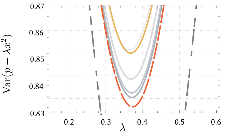
Supplementary Figure S3-2: Convergence of the Suzuki-Trotter approximation. Gray dot-dashed line represents the ideal unitary nonlinearity. Red dashed line comes from simulation in Fock space. Yellow is Method 2 with Trotter number $N=36$. Different shades of gray is Method 1 with Trotter number $N=6,12,24,36$. As $N$ increases, the color becomes darker.

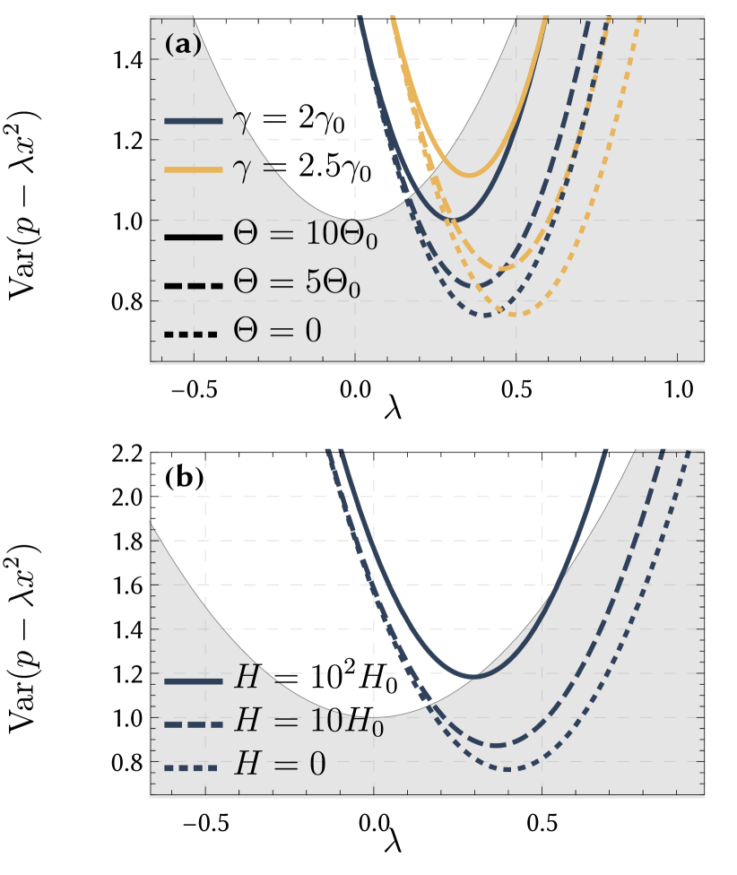
Supplementary Figure S4-2: Robustness of the nonlinear squeezing against main imperfections for the cubic potential $V(x)\propto\gamma x^{3}$. (a) Robustness against the duration $\Theta$ of quadratic evolution for different values of nonlinear gain $\gamma$. The mechanical oscillator is initialized in a squeezed thermal state (mean occupation $n_{0}=0.05$, squeezing $s=1.2$) and evolves according to (15) where $\Omega_{\mathsf{m}}\tau=\Theta$. Parameters same as in Fig. 2 $\gamma_{0}=0.2$, $\Theta_{0}=\pi/100$. (b) Robustness against thermal noise for different values of heating rate $H_{\mathsf{m}}$. After the evolution illustrated in (a), the mechanics is subject to thermal environment for a half of oscillation period. The parameters are $H_{0}=0.002$, $\gamma=2\gamma_{0}$, $\Theta=5\Theta_{0}$. Thin gray line shows variance computed at vacuum state, values below (filled area) provide advantage over vacuum as a resource for implementation of a measurement-based gate [52].

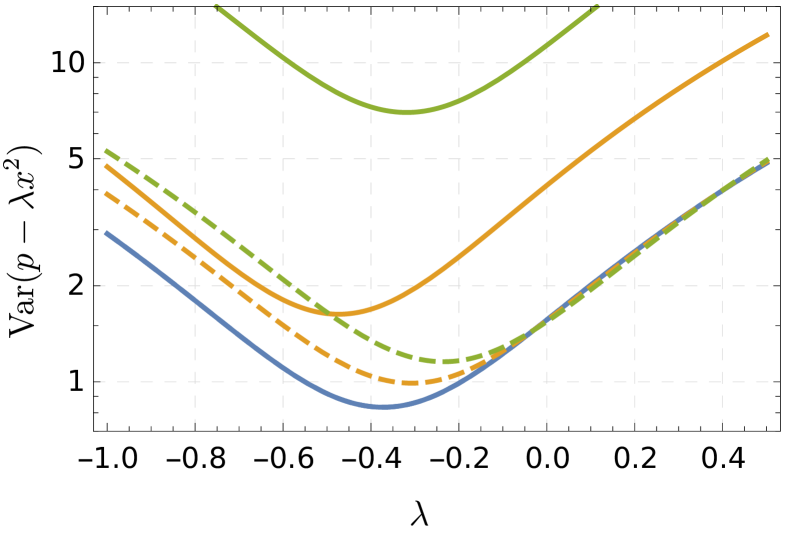
Supplementary Figure S5-2: Nonlinear squeezing for increased duration of the nonlinearity following different approaches. Solid lines, following Eq. S39-22: duration increases preserving the stiffness of nonlinearity. Dashed lines, following Eq. S40-22: duration increases keeping the nonlinear gain intact. Different colors correspond to duration $\tau^{\prime}$ proportionally increased compared to the value $\tau_{0}$ from main text. Blue lines $\tau^{\prime}=\tau_{0}$, yellow: $\tau^{\prime}=2\tau_{0}$, green: $\tau^{\prime}=3\tau_{0}$. As $\tau^{\prime}$ increases further, both methods approach the result of a noisy thermal mechanical state.

References

- [1] Samuel Braunstein and Peter van Loock “Quantum Information with Continuous Variables” In Rev. Mod. Phys. 77.2, 2005, pp. 513–577 DOI: 10.1103/RevModPhys.77.513
- [2] Seth Lloyd and Samuel L. Braunstein “Quantum Computation over Continuous Variables” In Phys. Rev. Lett. 82.8, 1999, pp. 1784–1787 DOI: 10.1103/PhysRevLett.82.1784
- [3] Daniel Gottesman, Alexei Kitaev and John Preskill “Encoding a Qubit in an Oscillator” In Phys. Rev. A 64.1, 2001, pp. 012310 DOI: 10.1103/PhysRevA.64.012310
- [4] Seckin Sefi and Peter van Loock “How to Decompose Arbitrary Continuous-Variable Quantum Operations” In Phys. Rev. Lett. 107.17, 2011, pp. 170501 DOI: 10.1103/PhysRevLett.107.170501
- [5] Jacob Hastrup et al. “Unsuitability of Cubic Phase Gates for Non-Clifford Operations on Gottesman-Kitaev-Preskill States” In Phys. Rev. A 103.3 American Physical Society, 2021, pp. 032409 DOI: 10.1103/PhysRevA.103.032409
- [6] Nadine Meyer et al. “Resolved-Sideband Cooling of a Levitated Nanoparticle in the Presence of Laser Phase Noise” In Phys. Rev. Lett. 123.15, 2019, pp. 153601 DOI: 10.1103/PhysRevLett.123.153601
- [7] Daniel Goldwater et al. “Levitated Electromechanics: All-Electrical Cooling of Charged Nano- and Micro-Particles” In Quantum Sci. Technol. 4.2, 2019, pp. 024003 DOI: 10.1088/2058-9565/aaf5f3
- [8] A. Vinante et al. “Ultralow Mechanical Damping with Meissner-Levitated Ferromagnetic Microparticles” In Phys. Rev. Applied 13.6 American Physical Society, 2020, pp. 064027 DOI: 10.1103/PhysRevApplied.13.064027
- [9] Markus Aspelmeyer, Tobias J. Kippenberg and Florian Marquardt “Cavity Optomechanics” In Rev. Mod. Phys. 86.4, 2014, pp. 1391–1452 DOI: 10.1103/RevModPhys.86.1391
- [10] “Cavity Optomechanics (Book)” Springer, 2014
- [11] Warwick P. Bowen and Gerard J. Milburn “Quantum Optomechanics” CRC Press, 2015
- [12] Farid Ya. Khalili and Stefan L. Danilishin “Quantum Optomechanics” In Progress in Optics 61 Elsevier, 2016, pp. 113–236
- [13] J.. Teufel et al. “Sideband Cooling of Micromechanical Motion to the Quantum Ground State” In Nature 475.7356, 2011, pp. 359–363 DOI: 10.1038/nature10261
- [14] Jasper Chan et al. “Laser Cooling of a Nanomechanical Oscillator into Its Quantum Ground State” In Nature 478.7367, 2011, pp. 89–92 DOI: 10.1038/nature10461
- [15] E.. Wollman et al. “Quantum Squeezing of Motion in a Mechanical Resonator” In Science 349.6251, 2015, pp. 952–955 DOI: 10.1126/science.aac5138
- [16] J.-M. Pirkkalainen et al. “Squeezing of Quantum Noise of Motion in a Micromechanical Resonator” In Phys. Rev. Lett. 115.24, 2015, pp. 243601 DOI: 10.1103/PhysRevLett.115.243601
- [17] Ralf Riedinger et al. “Remote Quantum Entanglement between Two Micromechanical Oscillators” In Nature 556.7702, 2018, pp. 473–477 DOI: 10.1038/s41586-018-0036-z
- [18] C.. Ockeloen-Korppi et al. “Stabilized Entanglement of Massive Mechanical Oscillators” In Nature 556.7702, 2018, pp. 478–482 DOI: 10.1038/s41586-018-0038-x
- [19] P.. Barker and M.. Shneider “Cavity Cooling of an Optically Trapped Nanoparticle” In Phys. Rev. A 81.2, 2010, pp. 023826 DOI: 10.1103/PhysRevA.81.023826
- [20] D.. Chang et al. “Cavity Opto-Mechanics Using an Optically Levitated Nanosphere” In Proc. Natl. Acad. Sci. 107.3, 2010, pp. 1005–1010 DOI: 10.1073/pnas.0912969107
- [21] O. Romero-Isart et al. “Optically Levitating Dielectrics in the Quantum Regime: Theory and Protocols” In Phys. Rev. A 83.1, 2011, pp. 013803 DOI: 10.1103/PhysRevA.83.013803
- [22] James Millen and Benjamin A. Stickler “Quantum Experiments with Microscale Particles” In Contemp. Phys. 61.3 Taylor & Francis, 2020, pp. 155–168 DOI: 10.1080/00107514.2020.1854497
- [23] David C. Moore, Alexander D. Rider and Giorgio Gratta “Search for Millicharged Particles Using Optically Levitated Microspheres” In Phys. Rev. Lett. 113.25, 2014, pp. 251801 DOI: 10.1103/PhysRevLett.113.251801
- [24] Gambhir Ranjit, Mark Cunningham, Kirsten Casey and Andrew A. Geraci “Zeptonewton Force Sensing with Nanospheres in an Optical Lattice” In Phys. Rev. A 93.5, 2016, pp. 053801 DOI: 10.1103/PhysRevA.93.053801
- [25] Jan Gieseler, Lukas Novotny and Romain Quidant “Thermal Nonlinearities in a Nanomechanical Oscillator” In Nat. Phys. 9.12, 2013, pp. 806–810 DOI: 10.1038/nphys2798
- [26] F. Ricci et al. “Optically Levitated Nanoparticle as a Model System for Stochastic Bistable Dynamics” In Nat Commun 8, 2017, pp. 15141 DOI: 10.1038/ncomms15141
- [27] Jan Gieseler and James Millen “Levitated Nanoparticles for Microscopic Thermodynamics - A Review” In Entropy 20.5, 2018, pp. 326 DOI: 10.3390/e20050326
- [28] Oriol Romero-Isart “Quantum Superposition of Massive Objects and Collapse Models” In Phys. Rev. A 84.5, 2011, pp. 052121 DOI: 10.1103/PhysRevA.84.052121
- [29] James Bateman, Stefan Nimmrichter, Klaus Hornberger and Hendrik Ulbricht “Near-Field Interferometry of a Free-Falling Nanoparticle from a Point-like Source” In Nat Commun 5, 2014, pp. 4788 DOI: 10.1038/ncomms5788
- [30] Daniel Goldwater, Mauro Paternostro and P.. Barker “Testing Wave-Function-Collapse Models Using Parametric Heating of a Trapped Nanosphere” In Phys. Rev. A 94.1, 2016, pp. 010104 DOI: 10.1103/PhysRevA.94.010104
- [31] Sougato Bose et al. “Spin Entanglement Witness for Quantum Gravity” In Phys. Rev. Lett. 119.24, 2017, pp. 240401 DOI: 10.1103/PhysRevLett.119.240401
- [32] C. Marletto and V. Vedral “Gravitationally Induced Entanglement between Two Massive Particles Is Sufficient Evidence of Quantum Effects in Gravity” In Phys. Rev. Lett. 119.24, 2017, pp. 240402 DOI: 10.1103/PhysRevLett.119.240402
- [33] Vijay Jain et al. “Direct Measurement of Photon Recoil from a Levitated Nanoparticle” In Phys. Rev. Lett. 116.24, 2016, pp. 243601 DOI: 10.1103/PhysRevLett.116.243601
- [34] Jamie Vovrosh et al. “Parametric Feedback Cooling of Levitated Optomechanics in a Parabolic Mirror Trap” In JOSA B 34.7, 2017, pp. 1421–1428 DOI: 10.1364/JOSAB.34.001421
- [35] Dominik Windey et al. “Cavity-Based 3D Cooling of a Levitated Nanoparticle via Coherent Scattering” In Phys. Rev. Lett. 122.12, 2019, pp. 123601 DOI: 10.1103/PhysRevLett.122.123601
- [36] Uroš Delić et al. “Cavity Cooling of a Levitated Nanosphere by Coherent Scattering” In Phys. Rev. Lett. 122.12, 2019, pp. 123602 DOI: 10.1103/PhysRevLett.122.123602
- [37] Uroš Delić et al. “Cooling of a Levitated Nanoparticle to the Motional Quantum Ground State” In Science 367.6480, 2020, pp. 892–895 DOI: 10.1126/science.aba3993
- [38] Henning Rudolph, Klaus Hornberger and Benjamin A. Stickler “Entangling Levitated Nanoparticles by Coherent Scattering” In Phys. Rev. A 101.1, 2020, pp. 011804 DOI: 10.1103/PhysRevA.101.011804
- [39] Andrey A. Rakhubovsky et al. “Detecting Nonclassical Correlations in Levitated Cavity Optomechanics” In Phys. Rev. Applied 14.5, 2020, pp. 054052 DOI: 10.1103/PhysRevApplied.14.054052
- [40] Antoine Bérut et al. “Experimental Verification of Landauer’s Principle Linking Information and Thermodynamics” In Nature 483.7388, 2012, pp. 187–189 DOI: 10.1038/nature10872
- [41] Artem Ryabov, Pavel Zemánek and Radim Filip “Thermally Induced Passage and Current of Particles in a Highly Unstable Optical Potential” In Phys. Rev. E 94.4, 2016, pp. 042108 DOI: 10.1103/PhysRevE.94.042108
- [42] Luca Ornigotti, Artem Ryabov, Viktor Holubec and Radim Filip “Brownian Motion Surviving in the Unstable Cubic Potential and the Role of Maxwell’s Demon” In Phys. Rev. E 97.3, 2018, pp. 032127 DOI: 10.1103/PhysRevE.97.032127
- [43] Martin Šiler et al. “Thermally Induced Micro-Motion by Inflection in Optical Potential” In Sci. Rep. 7.1, 2017, pp. 1697 DOI: 10.1038/s41598-017-01848-4
- [44] Martin Šiler et al. “Diffusing up the Hill: Dynamics and Equipartition in Highly Unstable Systems” In Phys. Rev. Lett. 121.23, 2018, pp. 230601 DOI: 10.1103/PhysRevLett.121.230601
- [45] M. Konopik, A. Friedenberger, N. Kiesel and E. Lutz “Nonequilibrium Information Erasure below kTln2” In EPL (Europhys. Lett.) 131.6, 2020, pp. 60004 DOI: 10.1209/0295-5075/131/60004
- [46] V.. Braginsky, Yu.. Vorontsov and F.. Khalili “Optimal Quantum Measurements in Detectors of Gravitation Radiation” In JETP Lett. 27, 1978, pp. 276
- [47] Carlton M. Caves et al. “On the Measurement of a Weak Classical Force Coupled to a Quantum-Mechanical Oscillator. I. Issues of Principle” In Rev. Mod. Phys. 52.2, 1980, pp. 341–392 DOI: 10.1103/RevModPhys.52.341
- [48] Masuo Suzuki “Generalized Trotter’s Formula and Systematic Approximants of Exponential Operators and Inner Derivations with Applications to Many-Body Problems” In Comm. Math. Phys. 51.2, 1976, pp. 183–190 DOI: 10.1007/BF01609348
- [49] Stephen D. Bartlett and Barry C. Sanders “Universal Continuous-Variable Quantum Computation: Requirement of Optical Nonlinearity for Photon Counting” In Phys. Rev. A 65.4, 2002, pp. 042304 DOI: 10.1103/PhysRevA.65.042304
- [50] Shohini Ghose and Barry C. Sanders “Non-Gaussian Ancilla States for Continuous Variable Quantum Computation via Gaussian Maps” In J. Modern Opt. 54.6, 2007, pp. 855–869 DOI: 10.1080/09500340601101575
- [51] Kazunori Miyata et al. “Implementation of a Quantum Cubic Gate by an Adaptive Non-Gaussian Measurement” In Phys. Rev. A 93.2, 2016, pp. 022301 DOI: 10.1103/PhysRevA.93.022301
- [52] Petr Marek et al. “General Implementation of Arbitrary Nonlinear Quadrature Phase Gates” In Phys. Rev. A 97.2, 2018, pp. 022329 DOI: 10.1103/PhysRevA.97.022329
- [53] V.V. Sivak et al. “Kerr-Free Three-Wave Mixing in Superconducting Quantum Circuits” In Phys. Rev. Applied 11.5 American Physical Society, 2019, pp. 054060 DOI: 10.1103/PhysRevApplied.11.054060
- [54] Matteo Brunelli, Daniel Malz, Albert Schliesser and Andreas Nunnenkamp “Stroboscopic Quantum Optomechanics” In Phys. Rev. Research 2.2, 2020, pp. 023241 DOI: 10.1103/PhysRevResearch.2.023241
- [55] Thomas Corbitt et al. “An All-Optical Trap for a Gram-Scale Mirror” In Phys. Rev. Lett. 98.15, 2007, pp. 150802 DOI: 10.1103/PhysRevLett.98.150802
- [56] Suresh Sridaran and Sunil A. Bhave “Electrostatic Actuation of Silicon Optomechanical Resonators” In Opt. Express 19.10, 2011, pp. 9020–9026 DOI: 10.1364/OE.19.009020
- [57] David Mason et al. “Continuous Force and Displacement Measurement below the Standard Quantum Limit” In Nat. Phys., 2019, pp. 1 DOI: 10.1038/s41567-019-0533-5
- [58] Lucas Lamata, Adrian Parra-Rodriguez, Mikel Sanz and Enrique Solano “Digital-Analog Quantum Simulations with Superconducting Circuits” In Adv. Phys. X 3.1, 2018, pp. 1457981 DOI: 10.1080/23746149.2018.1457981
- [59] Pavel Lougovski et al. “Digital-Analog Quantum Computation” In Phys. Rev. A 101.2 American Physical Society, 2020, pp. 022305 DOI: 10.1103/PhysRevA.101.022305
- [60] J. Weinbub and D.. Ferry “Recent Advances in Wigner Function Approaches” In Appl. Phys. Rev. 5.4 American Institute of Physics, 2018, pp. 041104 DOI: 10.1063/1.5046663
- [61] Jun-ichi Yoshikawa et al. “Creation, Storage, and On-Demand Release of Optical Quantum States with a Negative Wigner Function” In Phys. Rev. X 3.4, 2013, pp. 041028 DOI: 10.1103/PhysRevX.3.041028
- [62] D. Kienzler et al. “Observation of Quantum Interference between Separated Mechanical Oscillator Wave Packets” In Phys. Rev. Lett. 116.14, 2016, pp. 140402 DOI: 10.1103/PhysRevLett.116.140402
- [63] Chen Wang et al. “A Schrödinger Cat Living in Two Boxes” In Science 352.6289, 2016, pp. 1087–1091 DOI: 10.1126/science.aaf2941
- [64] K.. Johnson et al. “Ultrafast Creation of Large Schrödinger Cat States of an Atom” In Nat Commun 8.1, 2017, pp. 697 DOI: 10.1038/s41467-017-00682-6
- [65] Mitsuyoshi Yukawa et al. “Emulating Quantum Cubic Nonlinearity” In Phys. Rev. A 88.5, 2013, pp. 053816 DOI: 10.1103/PhysRevA.88.053816
- [66] Darren W. Moore, Andrey A. Rakhubovsky and Radim Filip “Estimation of Squeezing in a Nonlinear Quadrature of a Mechanical Oscillator” In New J. Phys. 21.11, 2019, pp. 113050 DOI: 10.1088/1367-2630/ab5690
- [67] Wolfgang P. Schleich “Quantum Optics in Phase Space” John Wiley & Sons, 2011
- [68] L.. Ballentine and S.. McRae “Moment Equations for Probability Distributions in Classical and Quantum Mechanics” In Phys. Rev. A 58.3 American Physical Society, 1998, pp. 1799–1809 DOI: 10.1103/PhysRevA.58.1799
- [69] David Brizuela “Classical and Quantum Behavior of the Harmonic and the Quartic Oscillators” In Phys. Rev. D 90.12 American Physical Society, 2014, pp. 125018 DOI: 10.1103/PhysRevD.90.125018
- [70] David Brizuela “Statistical Moments for Classical and Quantum Dynamics: Formalism and Generalized Uncertainty Relations” In Phys. Rev. D 90.8 American Physical Society, 2014, pp. 085027 DOI: 10.1103/PhysRevD.90.085027
- [71] Nikolai Kiesel et al. “Cavity Cooling of an Optically Levitated Submicron Particle” In Proc. Natl. Acad. Sci. 110.35, 2013, pp. 14180–14185 DOI: 10.1073/pnas.1309167110
- [72] Lorenzo Magrini et al. “Near-Field Coupling of a Levitated Nanoparticle to a Photonic Crystal Cavity” In Optica 5.12, 2018, pp. 1597–1602 DOI: 10.1364/OPTICA.5.001597
- [73] Lukas Martinetz et al. “Quantum Electromechanics with Levitated Nanoparticles” In npj Quantum Inf. 6.1 Nature Publishing Group, 2020, pp. 1–8 DOI: 10.1038/s41534-020-00333-7
- [74] M.. Vanner, I. Pikovski and M.. Kim “Towards Optomechanical Quantum State Reconstruction of Mechanical Motion” In Ann. Phys. 527.1-2, 2015, pp. 15–26 DOI: 10.1002/andp.201400124
- [75] Radim Filip and Andrey A. Rakhubovsky “Transfer of Non-Gaussian Quantum States of Mechanical Oscillator to Light” In Phys. Rev. A 92.5, 2015, pp. 053804 DOI: 10.1103/PhysRevA.92.053804
- [76] Petr Marek, Radim Filip and Akira Furusawa “Deterministic Implementation of Weak Quantum Cubic Nonlinearity” In Phys. Rev. A 84.5, 2011, pp. 053802 DOI: 10.1103/PhysRevA.84.053802
- [77] Keye Zhang, Francesco Bariani and Pierre Meystre “Quantum Optomechanical Heat Engine” In Phys. Rev. Lett. 112.15, 2014, pp. 150602 DOI: 10.1103/PhysRevLett.112.150602
- [78] Andreas Dechant, Nikolai Kiesel and Eric Lutz “All-Optical Nanomechanical Heat Engine” In Phys. Rev. Lett. 114.18, 2015, pp. 183602 DOI: 10.1103/PhysRevLett.114.183602
- [79] D. Rugar, R. Budakian, H.. Mamin and B.. Chui “Single Spin Detection by Magnetic Resonance Force Microscopy” In Nature 430.6997, 2004, pp. 329–332 DOI: 10.1038/nature02658
- [80] C.. Degen et al. “Nanoscale Magnetic Resonance Imaging” In Proc. Natl. Acad. Sci. 106.5, 2009, pp. 1313–1317 DOI: 10.1073/pnas.0812068106
- [81] Harry J.. Miller, Giacomo Guarnieri, Mark T. Mitchison and John Goold “Quantum Fluctuations Hinder Finite-Time Information Erasure near the Landauer Limit” In Phys. Rev. Lett. 125.16 American Physical Society, 2020, pp. 160602 DOI: 10.1103/PhysRevLett.125.160602
- [82] M.. Simón, M. Palmero, S. Martinez-Garaot and J.. Muga “Trapped-Ion Fock-State Preparation by Potential Deformation” In Phys. Rev. Research 2.2, 2020, pp. 023372 DOI: 10.1103/PhysRevResearch.2.023372
- [83] M. Abdi et al. “Dissipative Optomechanical Preparation of Macroscopic Quantum Superposition States” In Phys. Rev. Lett. 116.23 American Physical Society, 2016, pp. 233604 DOI: 10.1103/PhysRevLett.116.233604
- [84] Christopher Gerry and Peter Knight “Introductory Quantum Optics” Cambridge: Cambridge University Press, 2004 DOI: 10.1017/CBO9780511791239
- [85] T.. Palomaki, J.. Teufel, R.. Simmonds and K.. Lehnert “Entangling Mechanical Motion with Microwave Fields” In Science 342.6159, 2013, pp. 710–713 DOI: 10.1126/science.1244563
- [86] Brian C. Hall “Quantum Theory for Mathematicians” Springer Science & Business Media, 2013