Laser induced plasma expansion in quantum plasma

Abstract

Interaction of ultera-short laser pulses with a dense cold plasma is investigated. Due to high density, of plasma, quantum effects such that Bohm potential and quantum pressure should be considered. The results reveal that electron density function modulated by laser light in the propagation direction. This modulation can be controlled by amplitude of laser intensity and plasma effective parameters. For some special values of involved parameters electron density become localized in quenches spatially. Increasing the quantum coefficient tends to rarefy the high electron density regions, since the total number of electrons are constant. Hence, our theory predicts plasma expansion in the direction of laser light due to quantum effects.

I Introduction

Recently, there has been a growing interest in investigating new aspects of dense quantum plasmas Ref1 . Quantum plasmas have been achieved in nano-scale objects such as nano-wires, quantum dots, quantum wells, and semiconductor devices, as well as in laser plasma interaction Ref2 and wide interest due to their applications to astrophysical and cosmological environments Ref3 . Usually, the quantum plasma is characterized by a low-temperature and high-density plasma Ref4 , when mean inter-particle distance is comparable with the deBorglie thermal wavelength of plasma. Dense quantum plasma could be described by quantum hydrodynmics eqs.Ref5 ; Ref6 and quantum kinetic Eqs., including quantum forces which are associated by Bohm potential Ref5 and quantum pressure (due to degenerate electrons) which can be derived from Dirac’s equation Ref7 ; Ref8 ; Ref9 . On the other hand, Jung et.al show that when a laser pulse interacts with a cold dense quantum plasma, new quantum feature appears Ref10 . This new quantum feature is magnetization of plasma by photons which can be derived by considering a fiction time-dependent ponderomotive force. Considering this new quantum aspect we obtain an electron density distribution function for a cold isothermal dense quantum plasma illuminated by an ultra-short intense laser pulse. The result reveal that density bunching effects occurs in high laser intensities and for higher amount of quantum parameters. Our results predict plasma expansion due to quantum effects. This paper is organized in four sections. In section 2, we have explained the models of interaction of laser pulse with isothermal plasma. The basic equations and fundamental assumptions are given for this model. In section 3, the profiles of the electric field and variation of electron density are derived. Finally, section 4 is devoted to conclusion.

II Model description

In this section we are going to analyze propagation of an intense laser pulse through underdense collosionless quantum plasma in the non-relativistic regime. The temperature of electrons is held constant during the evolution. In this model, we consider a linearly x-polarized Gaussian laser pulse with time duration, $\tau$, propagation in +z direction in vacuum. The electron field of laser is written as:

$$E(z,t)=\hat{x}E(z)e^{-i\omega t}=\hat{x}E_{0}(z)e^{-\frac{t^{2}}{\tau^{2}}}e^{-i\omega t}$$ (1)

where $\omega$ is central angular frequency of the pulse. The $z>0$ region is taken to be filled with a homogeneous density profile of plasma with a plasma-vacuum interface placed at z=0. The electromagnetic incident the plasma region normally. Propagation of laser light in quantum plasma is governed by Maxwell’s equations:

$$\overrightarrow{\nabla}\times\overrightarrow{E}=-\frac{1}{c}\frac{\partial\overrightarrow{B}}{\partial t},$$ (2)

$$\overrightarrow{\nabla}\times\overrightarrow{B}=-\frac{1}{c}\frac{\partial\overrightarrow{E}}{\partial t}+\frac{4\pi}{c}\overrightarrow{J},$$ (3)

$$\overrightarrow{\nabla}.\overrightarrow{E}=4\pi\rho,$$ (4)

$$\overrightarrow{\nabla}.\overrightarrow{B}=0.$$ (5)

Here, $\overrightarrow{J}=-n_{e}e\overrightarrow{\vartheta_{e}}$ is the electron current density. By taking into account Eqs. (2-5), and defining function $\Omega(t)=\omega+\frac{2t}{i\tau^{2}}$, for further simplicity we have:

$$\frac{-\partial E_{x}}{\partial z}=-i\frac{(\Omega(t)+\dot{\Omega}(t)t)^{2}+2i\dot{\Omega}(t)}{c}B_{y},$$ (6)

$$\frac{-\partial B_{y}}{\partial z}=-i\frac{(\Omega(t)+\dot{\Omega}(t)t)^{2}+2i\dot{\Omega}(t)}{c}E_{x}-\frac{4\pi}{c}n_{e}e\vartheta_{x}.$$ (7)

Where, $E_{x}$, $B_{y}$ and $\vartheta_{x}$ are the component of electric field in x-direction, the component of magnetic field in y-direction and electron velocity in x-direction. Differentiating Eq. (6) with respect to z and substituting it into Eq. (7), we obtain a reduced (Helmholtz) differential equation for electric field in plasma:

$$\frac{d^{2}}{dz^{2}}E_{x}+[\frac{(\Omega(t)+\dot{\Omega}(t)t)^{2}+2i\dot{\Omega}(t)}{c^{2}}]\epsilon E_{x}=0.$$ (8)

On the other hand the electron’s equation of motion in collisionless quantum plasma can be expressed as Ref11 :

$$m_{e}n_{e}[\frac{\partial\overrightarrow{\vartheta_{e}}}{\partial t}+(\overrightarrow{\vartheta_{e}}.\overrightarrow{\nabla})\overrightarrow{\vartheta_{e}}]=-en_{e}\overrightarrow{E}-en_{e}\frac{\overrightarrow{\vartheta_{e}}\times\overrightarrow{B}}{c}-n_{e}e\overrightarrow{\nabla}\phi-\overrightarrow{\nabla}P_{e}-\overrightarrow{\nabla}P_{q}$$ (9)

where, $m_{e}$ and $P_{e}=n_{e}T_{e}$ are electron mass and pressure of electron respectively. $\phi=\frac{eE_{x}^{2}}{m_{e}\omega^{2}}$ is the average ponderomotive potential defined by the laser pulse envelope, with its corresponding ponderomotive force:

$$\overrightarrow{f_{P}}=-n_{e}e\overrightarrow{\nabla}\phi.$$ (10)

Moreover, $P_{q}$ is quantum pressure including Bohm potential and pressure resulted from electron degeneracy. Electron degeneracy pressure stems to Heisenberg’s uncertainty relation. Uncertainty of position and momentum implies that electron momentum is ill-defined and hence electron continuesly move around its occupied position. This phenomenon exerts pressure on surrounding medium which called electron degeneracy pressure. According to Ref12 ; Ref13 we can write:

$$\overrightarrow{\nabla}P_{q}=\frac{\hbar^{2}}{2m_{e}}\overrightarrow{\nabla}(\frac{\overrightarrow{\nabla^{2}}\sqrt{n_{e}}}{\sqrt{n_{e}}})-m\overrightarrow{\vartheta_{F}^{2}}\overrightarrow{\nabla}n^{(1)},$$

where $n_{e}=n_{e}^{(0)}+n^{(1)}$, here $\overrightarrow{\vartheta_{F}}$ is Fermi’s velocity. In the following the motion in different direction can be written in the $1^{ST}$ order approximation as:

$$m_{e}(\frac{\partial\vartheta_{x}}{\partial t})=-eE_{x},$$ (11)

$$-\frac{eB_{0}\vartheta_{x}}{c}-\frac{e\partial\phi}{\partial z}-\frac{1}{n_{e}}\frac{dP_{e}}{dz}-\frac{1}{n_{e}}\frac{dP_{q}}{dz}=0.$$ (12)

Where $B_{0}$ and $n_{0e}$ are refereed to external magnetic field (which is considered in the direction of laser field) and the maximum electron density respectively. By using Eqs. (8-12) we have:

$$\frac{\partial}{\partial z}[\frac{-e^{2}E^{2}_{x}-B_{0}B_{y}}{2m_{e}^{2}(\Omega(t))^{2}\Omega_{q}}]=\frac{\overrightarrow{\nabla}n_{e}}{n_{e}}$$ (13)

And hence:

$$n_{e}=n_{0e}exp[\frac{-e^{2}(E^{2}_{x}-B_{0}B_{y})}{2m_{e}^{2}(\Omega(t))^{2}\Omega_{q}}].$$ (14)

This equation shows that the electron density distribution depends on the laser electric field $E^{2}_{x}$, laser magnetic field $B_{y}$ and external magnetic field $B_{0}$. When the electric and magnetic fields are zero in the Eq. (14), $n_{e}$ represents the maximum electron density as we expected. Also we defined $\Omega_{q}$ as:

$$\Omega_{q}=\frac{T_{e}}{m_{e}}+\overrightarrow{\vartheta_{F}^{2}}+\frac{\hbar^{2}K^{2}}{4m_{e}^{2}}.$$

The quantum mechanical effects are encapsulated in the last two terms of this equation. In the classical limit ($\hbar\rightarrow 0)$ the results of non-quantum plasma is achieved Ref14 . On the other hand, non-magnetized plasma $(B_{0}=0)$, Eq. (14) turned to:

$$n_{e}=n_{0e}exp[\frac{-e^{2}E^{2}_{x}}{2m_{e}^{2}(\Omega(t))^{2}\Omega_{q}}]$$ (15)

The results is in agreement with the results of ref Ref15 for non-magnetized case in the absence of quantum effects. In literature of this field, it is convent to start from $P_{e}=n_{e}T_{e}$ and $\overrightarrow{f_{P}}=\overrightarrow{\nabla}P_{e}$, to extract the electron density $n_{e}$ Ref16 ; Ref17 . Reversing this procedure and starting from $n_{e}$ from Eq. (15), and $P_{total}=P_{e}+P_{q}$ we can write:

$$\overrightarrow{f_{P}}=\overrightarrow{\nabla}P_{e}+\overrightarrow{\nabla}P_{q}$$ (16)

for quantum plasma. Is this Eq. (16) includes all important quantum effects? The answer is actually No! For example, the quantum mechanic predict an induced magnetic field due to considering quantum feature of plasma dielectric constant. Such induced magnetic fields are introduced in Ref10 . In this paper, firstly we show that this purely quantum mechanical induced magnetic field can be derived by considering a fiction time-dependent pondromotive force. In the following we try to associate a electron density function to the plasma which describes the interaction of laser with quantum plasma.

$$f_{P}^{(t)}=\frac{-e^{2}E^{2}_{x}}{2m_{e}^{2}(\Omega(t))^{2}\Omega_{q}}\frac{2k\omega_{p}^{2}}{(\Omega(t))^{3}}\frac{\partial|E|^{2}}{\partial t}$$ (17)

This ponderomotive force relates to the electron density $n_{e}$ via $\omega_{p}$, this fact increases complexity of calculation. In order to overcome to this problem we replace $\omega_{p}$ by $\omega_{p0}$ in the last equation. Considering this new type of ponderomotive force modifies Eqs. (13) and (16) as follow:

$$\frac{\partial}{\partial z}[\frac{-e^{2}E^{2}_{x}}{2m_{e}^{2}(\Omega(t))^{2}\Omega_{q}}]+\frac{\partial}{\partial t}[\frac{-e^{2}E^{2}_{x}}{2m_{e}^{2}(\Omega(t))^{2}\Omega_{q}}\frac{2k\omega_{p}^{2}}{(\Omega(t))^{3}}|E|^{2}]=\frac{\overrightarrow{\nabla}n_{e}}{n_{e}},$$ (18)

$$\overrightarrow{f}_{P}^{(s)}+\overrightarrow{f}_{P}^{(t)}=\overrightarrow{\nabla}P_{total}=\overrightarrow{\nabla}P_{e}+\overrightarrow{\nabla}P_{q}.$$ (19)

For unmagnetized quantum plasma ($B_{0}=0$), and for Gaussian laser pulse this equation leads to the following formula:

$$\frac{-e^{2}E^{2}_{x}}{2m_{e}^{2}(\Omega(t))^{2}\Omega_{q}}+\frac{2ie^{2}k_{z}\frac{\omega_{p}^{2}}{(\Omega(t))^{2}}}{2m_{e}^{2}(\Omega(t))^{2}\Omega_{q}}\int_{0}^{L}E^{2}_{x}|E|^{2}dz=ln\frac{n_{e}}{n_{0e}},$$ (20)

$$n_{e}=n_{0e}\hskip 0.56917ptexp(\frac{-a^{2}}{2}+2ib^{2}k_{z}\frac{c}{\Omega(t)}\int_{0}^{L\frac{\Omega(t)}{c}}\frac{-a^{2}}{2}|E|^{2}d\xi).$$ (21)

Where

$$a^{2}=\frac{e^{2}E_{x}^{2}}{m_{e}^{2}(\Omega(t))^{2}\Omega_{q}},\hskip 11.38109pt\xi=\frac{z\Omega(t)}{c},\hskip 11.38109ptand\hskip 11.38109ptb=\frac{\omega_{p}}{\Omega(t)}$$

are dimensionless variables. Starting from Eq. (1) for a exponentially descending field i.e. $E(z)=E_{0}e^{-\alpha z}(\alpha>0)$, ($\alpha$ is absorption coefficient of the medium with the dimension of $L^{-1}$), we have $\overrightarrow{E}=\hat{x}E_{0}e^{-i\beta Z}e^{-i\Omega(t)t}$, where $\beta=-i\alpha+k_{z}$ is complex-valued wave number. Hence,

$$|E|^{2}=exp(-\frac{2c\beta\xi}{\Omega(t)})I(0)$$

$$n_{e}=n_{0e}exp(\frac{-a^{2}}{2}+2ik_{z}\frac{\omega_{p}^{2}}{(\Omega(t))^{2}}I(0)\frac{c}{\Omega(t)}\int_{0}^{L\frac{\Omega(t)}{c}}\frac{-a^{2}}{2}exp(-\frac{2c\beta\xi}{\Omega(t)})d\xi).$$ (22)

By considering Eq. (8) and (22) dielectric constant of quantum plasma is derived as:

$$\varepsilon=1-\frac{\omega_{p0e}^{2}}{(\Omega(t))^{2}}exp(\frac{-a^{2}}{2}+2ik_{z}\frac{\omega_{p}^{2}}{(\Omega(t))^{2}}I(0)\frac{c}{\Omega(t)}\int_{0}^{L\frac{\Omega(t)}{c}}\frac{-a^{2}}{2}exp(-\frac{2c\beta\xi}{\Omega(t)})d\xi),$$ (23)

and ultimately Eqs. (8) and (22) yield governing differential equation of propagation as:

$$\frac{d^{2}a}{d\xi^{2}}+\frac{(\Omega(t)+\dot{\Omega}(t)t)^{2}+2i\dot{\Omega}(t)}{(\Omega(t))^{2}}\times$$

$$[1-\frac{\omega_{p0e}^{2}}{(\Omega(t))^{2}}exp(\frac{-a^{2}}{2}+2ik_{z}\frac{\omega_{p}^{2}}{(\Omega(t))^{2}}I(0)\frac{c}{\Omega(t)}\int_{0}^{L\frac{\Omega(t)}{c}}\frac{-a^{2}}{2}exp(-\frac{2c\beta\xi}{\Omega(t)})d\xi)]a=0.$$ (24)

Starting from Eq. (22) and by some algebra we can write:

$$n_{e}=n_{0e}exp[\frac{-a^{2}}{2}-(1+i(1+\pi))|W|exp(-2i\Omega(t)t)exp(i\pi)exp(-2|\beta|L(1+i)-1)]$$ (25)

Where $W=\frac{e^{2}E_{0}^{2}}{4m_{e}^{2}c\Omega_{q}}\frac{bd}{\beta}$ with $d=\frac{K_{z}I(0)c}{\Omega(t)}$. The quantum effect is encapsulated in W so we call W as quantum factor.

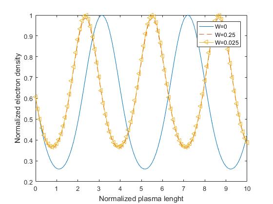
Figure 1: Vriations of normalized electrons density $\frac{n_{e}}{ne0}$ as a function of normalized plasma length $\frac{\Omega z}{c}$ inside isothermal plasma for different quantum coefficients W=0 (solid line), W=0.25 (dotted line), and W=0.025 (dashed line) for $a_{0}=1,b=0.1$.

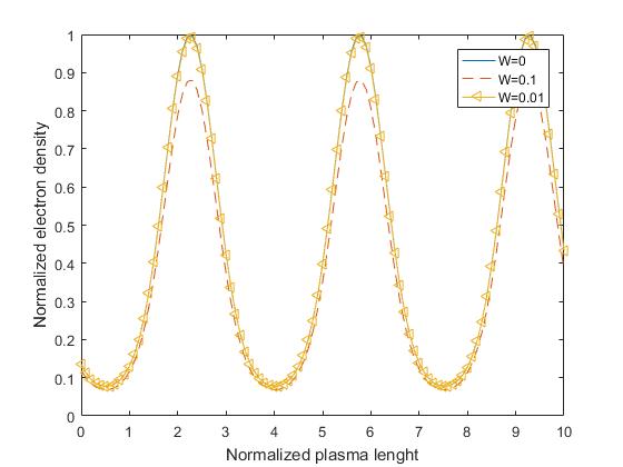
Figure 2: Vriations of normalized electrons density $\frac{n_{e}}{ne0}$ as a function of normalized plasma length $\frac{\Omega z}{c}$ inside isothermal plasma for different quantum coefficients W=0 (solid line), W=0.1 (dotted line), and W=0.01 (dashed line) for $a_{0}=2,b=0.1$.

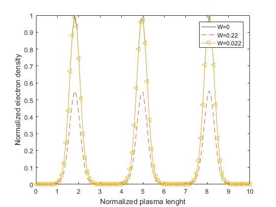
Figure 3: Vriations of normalized electrons density $\frac{n_{e}}{ne0}$ as a function of normalized plasma length $\frac{\Omega z}{c}$ inside isothermal plasma for different quantum coefficients W=0 (solid line), W=0.22 (dotted line), and W=0.022 (dashed line) for $a_{0}=3,b=0.1$.

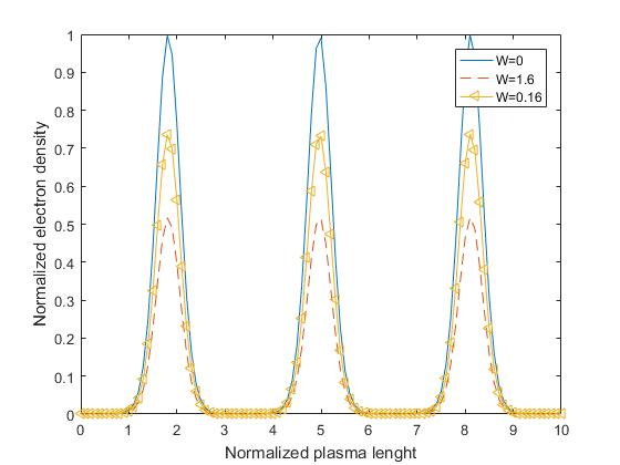
Figure 4: Vriations of normalized electrons density $\frac{n_{e}}{ne0}$ as a function of normalized plasma length $\frac{\Omega z}{c}$ inside isothermal plasma for different quantum coefficients W=0 (solid line), W=1.6 (dotted line), and W=0.16 (dashed line) for $a_{0}=4,b=0.4$.

III Results

Due to nonlinearity of governing Eq. (25), analytical trace of calculation is impossible. The results of numerical solution of Eq. (25) is illustrated in Fig. (1-4). In these figures we focus on the variation of electron density through the plasma. Figure are plotted for some values of laser intensity amplitude, size of quantum factor and b=$\frac{\omega_{p}}{\Omega(t)}$. These parameters are not independent (see definition of W), so changing one parameters affect the value of others. All of the figures, show that electrons accumulate in some region and hence some regions deplete from free electrons. The loci of these regions and their electron number can be altered by introducing quantum effects. This phenomenon intensively affects the transport process of the plasma (such as electrical conductivity and thermal conductivity). Figure (1) depicts that electron density function oscillates through the plasma in the direction of laser light. Quantum effects decreases the wavelength of this oscillation. Variation of normalized electron density versus normalized plasma length is illustrated in figure (2) for intermediate laser intensity. In this regime departure from classical plasma is not considerable. Increasing the intensity of laser light reveal quantum effects. Figures (3) and (4) show this fact. Further increasing of W, cause to decrease peak of $n_{e}$. Since the total electron number of plasma is constant, decreasing in $n_{e}$ is accombined by increasing the volume (length) of plasma. Also, for high intensities of laser light, similar to classical plasma $n_{e}$ completely localized in some regions in the direction of laser light. This fact my be is due to solitary solution of non-linear Eq. (24).

IV Conclusion

A new phenomenon is observed in the process of laser-plasma interaction. We claim that when an ultra-short Gaussian laser pulse interact with a quantum plasma. The size of plasma in the laser direction is changed. This phenomenon has various applications. For example it can be used in performance of Acousto-optical modulators (AOM).

References

• (1) D. Kremp, M. Schlanges, W.-D. Kraeft, Quantum statistics of Nonideal plasma, Springer-verlag, Berlin, 2005.
• (2) S. Son, Phys. Plasmas 21(3), 0345020 (2014).
• (3) A. K. Harding, and D. Lai, Rep. Prog. Phys. 69, 2631 (2006).
• (4) S. Ali, P. K. Shukla, Phys. Plasmas 13, 102112 (2006).
• (5) G. Manfredi, Fields Inst. Commun. 46, 263 (2005).
• (6) C. L. Gardner and C. Ringhofer, Phys. Rev. E 53, 157 (1996).
• (7) W. D. Kraeft, D. Kremp, W. Ebeling and G. Ropke, 1986 Quantum statistics of charge particle systems (Berlin: Akademie-verlag)
• (8) D. Kremp, M. Schlanges and W. D. Kraft 2005 Quantum Statistics of Nonideal plasmas (Berlin: Springer)
• (9) N. L. Tsintsadze and L. N. Tsintsadze EPL 88, 35001 (2009).
• (10) Y.-D. Jung, I. Murakami, Physics Letters A 373, 969-971 (2009).
• (11) H. Fernando, Quantum plasmas: An hydrodynamic approach (Springer Science and Business Media 2011)
• (12) P. K. Shukla, and B. Eliasson, Phys.-Usp 53, 51-76 (2010).
• (13) A. k. Singh, and S. Chandra, Laser and Particle Beams, 35(2), 252-258 (2017).
• (14) R. Sadighi-Bonabi, and M. Ettehadi-Abari Physics of Plasma 17, 032101 (2010).
• (15) M. Ettehadi-Abari et al 2015 Plasma Phys. Control. Fusion. 57, 085001 (2015).
• (16) V. Godyak, R. Piejak, B. Alexandrovich, and A. Smolyakov, Plasma Sources Sci. Technol. 10, 459 (2001).
• (17) V. Godyak, Plasma Phys. Control. Fusion. 45, A399 (2003).