Origin and evolution of long-period comets

Abstract

We develop an evolutionary model of the long-period comet (LPC) population, starting from their birthplace in a massive trans-Neptunian disk that was dispersed by migrating giant planets. Most comets that remain bound to the Solar system are stored in the Oort cloud. Galactic tides and passing stars make some of these bodies evolve into observable comets in the inner Solar system. Our approach models each step in a full-fledged numerical framework. Subsequent analysis consists of applying plausible fading models and computing the original orbits to compare with observations. Our results match the observed semimajor axis distribution of LPCs when Whipple’s power-law fading scheme with an exponent $\kappa=0.6^{+0.1}_{-0.2}$ is adopted. The cumulative perihelion ($q$) distribution is fit well by a linear increase plus a weak quadratic term. Beyond $q=15$ au, however, the population increases steeply and the isotropy of LPC orbital planes breaks. We find tentative evidence from the perihelion distribution of LPCs that the returning comets are depleted in supervolatiles and become active due to water ice sublimation for $q\leq 3$ au. Using an independent calibration of the population of the initial disk, our predicted LPC flux is smaller than observations suggest by a factor of $\simeq 2$. Current data only characterize comets from the outer Oort cloud (semimajor axes $\gtrsim 10^{4}$ au). A true boost in understanding the Oort cloud’s structure should result from future surveys when they detect LPCs with perihelia beyond $15$ au. Our results provide observational predictions of what can be expected from these new data.

1 Introduction

Comets are primitive bodies born mostly in a massive trans-Neptunian disk, though some might have formed in the region in between giant planets too. They share a birthplace with several other populations of small bodies in the outer Solar system, such as Jupiter and Neptune Trojans, the irregular satellites of giant planets, the resonant and hot components of the Kuiper belt, and objects in the scattering disk. Out of all these categories of small bodies, comets underwent the most spectacular orbital evolution before being observed. Except for those in the Jupiter family, comets were scattered by the giant planets to the very outskirts of the Solar system to form a storage zone called the Oort cloud. There, barely gravitationally bound to the Sun, comets wait eons for their chance to return to the inner regions of the Solar system. Assisted by galactic tides and tugs from passing stars, they eventually set on their journeys. They plunge into the planetary zone on highly eccentric orbits before disappearing forever (e.g. Dones et al., 2004). Obviously, their activity – namely, the production of gas and dust comae as they become heated by solar radiation when they get close enough to the Sun – makes them classified as comets in the first place and constitutes the glory of their deadly run.

Cometary precursors in the Oort cloud cannot be observed in situ. This holds even for the largest expected members in this population, which may be Pluto-sized, or even larger. Therefore, unraveling properties of the Oort cloud remains one of the great challenges in planetary science. They can only be inferred thus far from observations of comets that once visited the Oort cloud region. Halley-type comets (HTC) are less useful in this respect. This is because before being observed, HTCs underwent significant orbital evolution after leaving their source zone. Therefore, the long-period comets (LPCs) are a better tracer population of the Oort cloud. Using the commonly adopted definition, we define LPCs as comets with orbital periods longer than $200$ yr (thus heliocentric semimajor axis $a\gtrsim 35$ au). However, most LPCs reside on much more extreme orbits having $a$ equal to thousands or even tens of thousands of au. The equivalent orbital periods are as large as several million years. With these orbital parameters, LPCs can tell us a great deal about the Oort cloud architecture.

The fundamental facts about LPC orbits have been pinned down already by Oort (1950): (i) a preponderance of comets on nearly parabolic orbits, constituting what is now called the Oort peak, with the implication of strong fading during subsequent returns (see Section 3.6), (ii) near isotropy of the orbital planes in space, and (iii) nearly equal numbers of LPCs in equal bins of perihelia for $q<1.5$ au. It is somewhat surprising how little has been added to this broad picture on the observational side over the past decades, especially if compared with the vast increase of data about other populations of small bodies in the Solar system. The additions include (i) a more complete characterization of the returning population of LPCs on orbits more strongly bound to the Sun, and (ii) extension of the data set to larger perihelia. The paucity of new data is due, in part, because, until the late 1990s, only about a dozen or fewer new LPCs were discovered annually, many by amateurs, rather than by well-characterized surveys (http://comethunter.de/). The situation has improved in the past two decades, but a significant boost of new LPC discoveries by surveys is still in the future.

The theory side of LPC studies has evolved somewhat more. It has been understood that the inner edge of the Oort peak at about $10000$ au is simply an apparent structure due to a bias related to observing only comets with small perihelion distances (e.g., Hills, 1981). The inner Oort cloud is expected to extend to $\approx$ 3000 au from the Sun (e.g., Duncan et al., 1987), but comets from the inner cloud should only reach the inner Solar system during rare comet showers (e.g., Heisler et al., 1987; Heisler, 1990). The role of the Sun’s likely birth cluster, the Sun’s migration in the Galaxy, and planetary migration were all investigated. The dynamics of bodies stored in the Oort cloud was also understood by analyzing the effects of galactic tides and stellar short-range perturbations. Finally, other studies shed a detailed light on the transfer dynamics of comets into the heliocentric zone where they become observable. Reviews may be found in Dones et al. (2004), Rickman (2010) and Dones et al. (2015).

In spite of all these improvements, and partially because of lack of data, fewer studies were devoted to a direct comparison of theoretical predictions with LPC observations. An outstanding achievement in this respect was obtained by Wiegert & Tremaine (1999), who compared the available data to the state of the art in modeling of LPC dynamics. Still, this work adopted a number of simplifications. For instance, all available data were compressed into three measures which the authors confronted with model predictions: (i) the number of comets in the Oort peak vs. all LPCs, (ii) the number of comets in the small-semimajor axis tail (34.5 au$\lesssim a\lesssim 69$ au) vs. all LPCs, and (iii) the number of comets with retrograde orbits vs. all LPCs. These data constrain the model in its important aspects, yet they remain rather coarse. The numerical model used in Wiegert & Tremaine (1999) was obviously restricted by computer capabilities at that time, but it also neglected some important effects. For instance, prevailing opinion in the 1990s highlighted the effects of galactic tides over the perturbations due to passing stars. However, further analyses found about equal importance – or even a synergistic role – of both effects (e.g., Rickman et al., 2008).

Our goal in this work is to extend the effort of Wiegert & Tremaine (1999) in both aspects, namely orbital data and numerical model. As for the data side, we have now more complete information. Significant improvements especially concern the class of LPCs on near-parabolic orbits (Sec. 2.2). There have been new estimates of the annual flux of LPCs, though uncertainties still remain about the sizes of cometary nuclei (e.g., Francis, 2005; Brasser & Morbidelli, 2013). There has been again more improvement on the modeling side. Most importantly, today’s computer capabilities allow us to propagate (i) the orbits of millions of test particles from their ultimate birthplaces to the moments they become observable as comets some $4.5$ Gyr later, and (ii) use a single framework of a full-fledged N-body integrator (without switching between a secular approximation and an N-body calculation). A unique aspect of our approach consists of using initial orbital data for comets that reflect their true birth zone, which has been calibrated by other, independent applications of the model. Finally, our work complements the model presented in Nesvorný et al. (2017), where the origin and dynamical evolution of short-period comets was analyzed and confronted with observations. Therefore, it is for the first time – to our knowledge – that the same model is used to explain the properties of all comets.

In Section 2, we summarize observational data about LPCs. This has two facets: (i) orbital architecture, principally the semimajor axis distribution, complemented with information about perihelia and inclinations, and (ii) the observed flux of LPCs. We focus principally on orbits. This is because the flux information suffers uncertainty in the magnitude-size relation of these comets. In Section 3, we present our model. We highlight our beginning-to-end approach, following comets from their birth environment in a dynamically cold, trans-Neptunian disk of planetesimals to the Oort cloud and back to the observable zone. In Section 4, we describe results from our simulations. First, we characterize the orbits of new and returning comets in a chosen heliocentric target zone. We use heliocentric distances $r\leq 5$ au, relevant for the population of the currently observed LPCs, and $r\leq 20$ au, in anticipation of future surveys. Next, we compare simulations to the observations. Finally, in Section 5 we use our model to highlight a few predictions relevant for future surveys that should be able to detect LPCs with distant perihelia.

2 Properties of known LPCs

As we await powerful, well-characterized surveys that will provide accurate and homogeneous information on the orbital distribution and flux of LPCs, we are left with a sample obtained by many different sources and different observational circumstances, often analyzed by different computational methods. This inevitably implies biases which cannot be entirely removed. Cometary activity, especially at small heliocentric distances, does not help the situation. It not only necessitates including complicated nongravitational effects in the orbit determination, and thus characterization of the orbital binding energy with which the comet approached the inner Solar system, but it also makes it hard to determine the size of the nucleus.

With that gloomy preamble it is, however, true that tremendous steps forward have been taken over the past decades. These efforts started in the 1960s and resulted in the first population-wide orbital information about LPCs in the 1970s (e.g., Marsden & Sekanina, 1973; Marsden et al., 1978). Since then, Marsden and collaborators carried out continuous improvements in orbital characterization of LPCs, maintaining and periodically updating their catalog. The latest, 17th edition from 2008 (Marsden & Williams, 2008, MWC08) still represents the current state-of-the-art. In Sec. 2.1 we describe a subset of MWC08 that will be used for comparison with our modeled LPC population.

An effort specific to LPCs on nearly parabolic orbits, roughly speaking, those in the Oort peak with $a\gtrsim 15000$ au, has been conducted by a group of Polish astronomers since 1970. This work culminated with the publication of a catalog of their orbits by Królikowska et al. (2014) and Królikowska (2014), later complemented by an analysis of large-perihelion LPCs in Królikowska & Dybczyński (2017). A large fraction, between 20 to 50% (depending on perihelion distance), of entries in the catalog are comets with accurate orbits for which nongravitational effects were included in the orbit determination from the observations. Importantly, each orbital element, including those with which comets approached the Solar system, is provided with a statistical uncertainty (reflecting the specific orbital determination accuracy). The catalog is accompanied by a series of papers (e.g., Królikowska & Dybczyński, 2010; Dybczyński & Królikowska, 2011; Królikowska & Dybczyński, 2013; Dybczyński & Królikowska, 2015) which thoroughly describe various aspects of the past and future motion of very weakly-bound LPCs. Finally, this source contains comets observed through 2013, five years past the release of MWC08. In the case of comets on nearly parabolic orbits, we thus consider the Polish catalog as a superior source and describe its characteristics in Sec. 2.2.

The orbital catalogs mentioned above do not contain information about physical parameters of the comets (such as the absolute brightness and size), nor do they directly describe their flux to the inner parts of the Solar system. These data have to be inferred from other sources, some of which are recalled in Sec. 2.3.

2.1 Orbital characteristics of all LPCs

The MWC08 catalog contains information about the original orbits for 499 LPCs. Their orbital elements are (i) referred to the barycenter of the Solar system, and (ii) computed from state vectors (position and velocity) at a sufficiently large distance along the orbit prior to each comet’s passage through the planetary region (in MWC08 a distance of 60 au is used). This definition requires backward propagation of the osculating solution, determined from observations at small heliocentric distances, for at least the nominal orbit (ideally, though, also with mapping its uncertainty). The transformation between osculating (heliocentric) and original (barycentric) elements has the most profound effect on the orbital semimajor axis $a$: often a formally hyperbolic heliocentric orbit becomes elliptical. Other elements, such as perihelion distance $q$ and inclination $i$, are less affected. Since the source of LPCs is very distant from the inner parts of the Solar system, the barycentric orbital elements are the most relevant for their study. As a result, in what follows we shall always use the original orbital elements, including the semimajor axis, in our discussion (unless specifically mentioned otherwise).

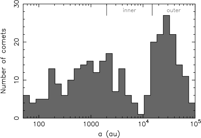
Figure 1: Distribution of semimajor axes $a$ of LPCs in the MWC08 catalog. Data for $318$ 1A and 1B orbits are used and plotted using equal size bins in ${\rm log}\,a$. The comets on nearly parabolic orbits, $a\gtrsim 15000$ au, have a source in the outer part of the Oort cloud. Comets having orbits with $a\lesssim 15000$ au generally are returning to the inner Solar system after they passed through the planetary zone at least once in the recent past.

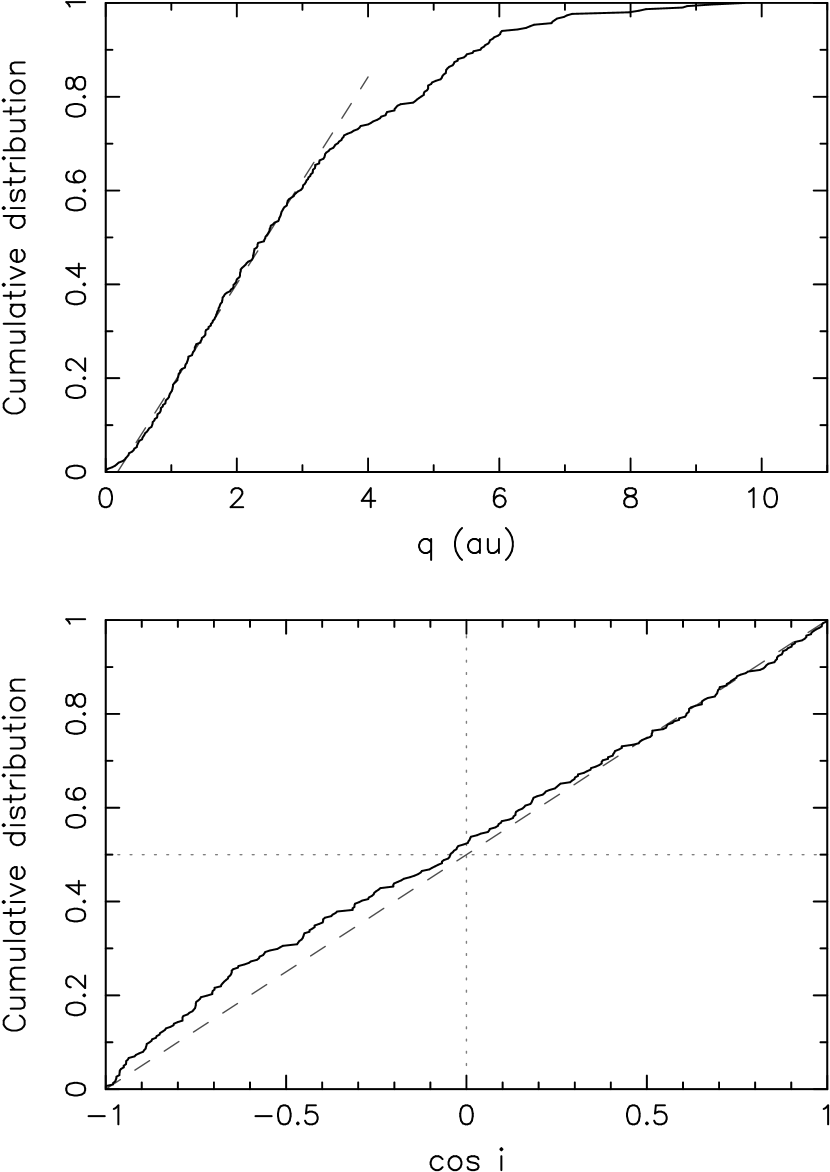
Figure 2: Cumulative distribution of perihelion distance $q$ (top) and cosine of inclination $\cos i$ with respect to the ecliptic plane (bottom) for the selected sample of $318$ 1A and 1B orbits in MWC08. The gray dashed line in the upper panel shows a linear approximation for $q\leq 3$ au for reference. The dashed gray line in the bottom panel corresponds to an isotropic distribution (dotted lines indicate polar orbits, $\cos i=0$, the median value for an isotropic distribution).

Given the wealth of data in MWC08, and being cautious about the biases mentioned above, we opted to analyze only the 1A- and 1B-flagged orbits (see, e.g., Marsden et al., 1978). This is a subset of 318 comets with the most accurately determined orbits in the catalog. Figure 1 shows the distribution of semimajor axis $a$ of this sample of MWC08 comets. Here we use ${\rm log}\,a$ as the abscissa instead of $1/a$, which is more suitable to study the sub-class of comets on nearly parabolic orbits (Sec. 2.2). This choice allows us to distinguish the population of returning comets with $a\lesssim 15000$ au from those from the canonical Oort peak with $a\gtrsim 15000$ au. We shall also occasionally denote the latter group as new comets, although both previous work (e.g., Kaib & Quinn, 2009; Dybczyński & Królikowska, 2011; Królikowska & Dybczyński, 2013; Dybczyński & Królikowska, 2015; Królikowska & Dybczyński, 2017) and our integrations show that a number of observed LPCs with $a\gtrsim 15000$ au have visited the planetary zone before. The fraction of observed LPCs in the Oort spike is $\simeq 37$% (also see Wiegert & Tremaine, 1999, who used the 1993 edition of the Marsden-Williams catalog of LPCs).

Figure 2 shows the cumulative distribution of perihelion distance $q$ and cosine of inclination $\cos i$ for the sample of $318$ new and returning comets from MWC08. The perihelion distribution is fairly well-matched by a linear fit up to $q\simeq 3$ au, with perhaps only a slight deficiency of the lowest-$q$ orbits ($\leq 0.2$ au, say). Beyond $3$ au, the distribution diverges from the linear trend and becomes shallower, likely due to biases in the data set (i.e., comets with larger perihelion distances are typically fainter and thus harder to discover). However, if we were to restrict ourselves to the subset of about 130 comets in the Oort peak ($a>12500$ au, say), the $q$- and $\cos i$-distributions would be consistent with those given in Fig. 4. In particular, the linear part of the $q$-distribution would extend to nearly $q\simeq 6$ au. We thus interpret the missing population of comets beyond $q\simeq 3$ au in the upper panel of Fig. 2 primarily as a deficiency of returning comets, perhaps due to fading of their brightness in subsequent returns. On a physically deeper level, such a fading pattern may result because the returning comets already exhausted their content of supervolatiles, which might have driven their huge activity on their first appearance. When these comets return, it may be primarily the water sublimation below $\simeq 3$ au which triggers their activity. Beyond Jupiter’s orbit, even new comets may be too faint to be detected by available surveys; only a small fraction of the known population of LPCs has $q>5$ au. There are also biases subtler than the obvious lack of large-perihelion comets. Note, for instance, that the linear progression of the cumulative $q$-distribution is expected at the crudest approximation (e.g., Fernández, 2005, pp. 127-130). Nevertheless, numerical models that take planetary perturbations into account (e.g., Wiegert & Tremaine, 1999; Fouchard et al., 2017a, and Sec. 4.2 below) predict a slightly nonlinear progression. This is not seen in the upper panel of Fig. 2, possibly because: (i) some comets are missing in the MWC08 sample even below $q\simeq 3$ au, and/or (ii) the sample is not homogenized to a common absolute brightness limit, such that a certain number of smaller (and intrinsically less bright) comets contribute at small $q$ values. We do not feel comfortable removing either of these possible effects.

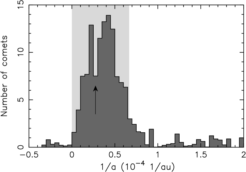
Figure 3: Distribution of binding energy for LPCs on nearly parabolic orbits expressed as $1/a$ values (positive for elliptic orbits, negative for hyperbolic orbits). We use 134 entries in the Królikowska et al. catalogs for which the stated uncertainty in $1/a$ is smaller that $10^{-5}$ au^-1 (this limiting value is twice as large as the bin size used). Each comet is represented by a Gaussian distribution with mean equal to the nominal value of $1/a$ and standard deviation of the uncertainty in $1/a$. The gray rectangle highlights what is traditionally described as the Oort peak ($a\gtrsim 15000$ au here).

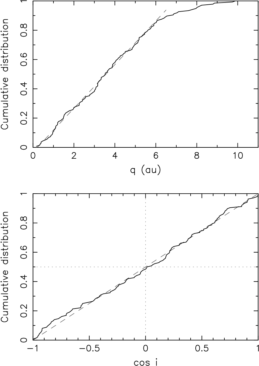
Figure 4: Cumulative distribution of perihelion distance $q$ (top) and cosine of inclination $\cos i$ with respect to the ecliptic plane (bottom) for the selected sample of $134$ accurate orbits in the Królikowska et al. catalogs of LPCs on nearly parabolic orbits. The dashed gray line in the upper panel shows a linear approximation for $q\leq 6$ au for reference. The dashed and gray line in the bottom panel correspond to an ideally isotropic distribution (dotted lines indicate polar orbits, $\cos i=0$, the median value for an isotropic distribution).

The inclination distribution seen in the lower panel of Fig. 2 is basically isotropic with only a slight excess of retrograde cases. Again, when only the Oort peak comets of the LPCs in MWC08 are used, the inclination distribution becomes closer to that of an isotropic population. We thus believe that the small excess of retrograde orbits originates primarily from the returning population of LPCs.

2.2 Orbital characteristics of nearly parabolic comets

As mentioned above, in order to describe comets on nearly parabolic orbits in the Oort peak, we use data collected by a group of Polish astronomers led by Królikowska. This represents a union of data published in Królikowska (2014), Królikowska et al. (2014) and Królikowska & Dybczyński (2017), altogether 186 comets. Each entry in this catalog, as used here, represents the orbital parameters of the original orbit together with the estimated uncertainty.

Figure 3 shows the distribution of semimajor axis $a$ as a function of $1/a$. Given a sufficiently large number of entries in the catalog, we again restricted ourselves to a set of the most accurately determined orbits. Here we only use those for which the uncertainty in $1/a$ does not exceed $10^{-5}$ au^-1, thus reducing the sample to 134 comets. According to methods in Królikowska (2014), and the following papers in their series, we represent each comet with a Gaussian having the mean and standard deviation from the catalog. These data were then represented as a histogram with bin size $5\times 10^{-6}$ au^-1, about the median uncertainty of the cometary data. The data show the structure of the Oort peak in a great deal of detail. Królikowska & Dybczyński (2017) note the division of the distribution by a dip at about $a\simeq 40000$ au (see the arrow in Fig. 3), and associate it with a separation of dynamically new and old orbits (see also Section 4.4.1).

Figure 4 shows the cumulative distribution of perihelion distance $q$ (top) and cosine of inclination $\cos i$ (bottom) for the selected sample of 134 nearly parabolic comets from the Królikowska et al. catalogs. When compared with Fig. 2, the behavior is now simpler: (i) the linear trend in $q$ continues to nearly $6$ au, before falling below the line, and (ii) the inclination distribution closely matches an isotropic population, with only small fluctuations. However, more subtle biases, such as the missing expected nonlinear contribution in the $q$-distribution discussed in the previous section, may still be present.

2.3 Cometary flux and size distribution

Unlike asteroids, comets hide the sizes of their nuclei with a huge range of activity when they become observable. This brings large difficulties in understanding their population parameters, in particular their size distribution and/or size-limited flux.

Comets’ intrinsic brightness is usually expressed in terms of the absolute total magnitude $H$, which is related to the apparent magnitude $m$ using a relation $H=m-5\,{\rm log}_{10}\,d-2.5\,n\,{\rm log}_{10}\,r$ (e.g., Fernández, 2005). (Cometary absolute magnitude determinations sometimes include a term that accounts for non-zero solar phase angle; we ignore this correction.) Here $d$ and $r$ are the geocentric and heliocentric distances, respectively, and $n$ is the photometric index, which strongly depends on the strength and nature of a given comet’s activity. For an inactive (asteroidal) body, $n=2$. Often $n=4$ is assumed for comets, leading to the conventional absolute magnitude $H_{\rm 10}$. However, comets show a great diversity in their activity and $n$ indexes ranging from $1$ to $10$ have been reported for different comets (with even more extreme values on occasion, e.g., Whipple, 1978). Additionally, in many cases photometric observations are not available for a large enough interval of heliocentric distances $r$, so that the $n$ value of a given comet is unknown. In this situation, $H_{\rm 10}$ is canonically considered as the cometary absolute magnitude and taken as a proxy for a physically more justified value of $H$. One should then understand that such values may cause significant biases.

Yet another difficulty stems from the relation between the absolute magnitude $H$ and the nucleus diameter $D$. This is because in nearly all situations the observed brightness of a long-period comet results from sunlight reflected by its large coma with basically no, or very little, contribution from the nucleus. Subtraction of the coma is a tricky business (see, e.g., Hui & Li, 2018).

To circumvent these troubles, Sosa & Fernández (2011) used a determination of non-gravitational forces in the motion of a sample of LPCs with $q<2$ au to infer their nuclear masses. By assuming a mean bulk density of $0.4$ g cm^-3, they were able to estimate the effective sizes of the nuclei. Running this analysis for a sample of $15$ well-observed LPCs, Sosa & Fernández (2011) were able to find an approximate relation between $H$ and $D$ for this class of comets: $\log_{10}D\simeq 1.2-0.13\,H$ [Note, however, that other authors have obtained similar relationships with different constants on the right hand side; see the review in Fernández (2005). If the light reflected by a comet is proportional to $D^{n}$, where $n$ is a constant, the coefficient of $H$ is $-0.4/n$. Thus the relation found by Sosa & Fernández (2011) implies $n\approx 3$, i.e., the reflected light is proportional to the volume of the nucleus, not its surface area. Weissman (1990) finds, based on 1P/Halley, that $\log_{10}D\simeq 1.9-0.13\,H$ (for a density of $0.4$ g cm^-3), which implies that comets are $\approx 5$ times bigger than one obtains using the Sosa & Fernández (2011) relation.] As an example, an $H=11$ magnitude comet would have, using the relation of Sosa & Fernández (2011), $D\simeq 600$ m. Fernández & Sosa (2012) used this analysis to infer that the size distribution of active LPCs may be shallow for $D\gtrsim 4.8$ km, steep between $\simeq 2.8$ km and $\simeq 4.8$ km, and shallow again between 1.2 and 2.8 km [for 1.2–2.8 km, $N(>D)\propto D^{-1.54\pm 0.15}$, where $N(D)$ is the cumulative number of nuclei with diameter larger than $D$], and even shallower for smaller nuclei. A possible caveat, not accounted for in the uncertainty budget, is that the analysis of Sosa & Fernández (2011) depends on the shape and location of active areas on the cometary nucleus. These factors are highly uncertain, especially for LPCs, and might affect their results.

Another, in principle more accurate, method would be to observe comets at very large heliocentric distances in both visible and infrared bands. Assuming no, or very small, activity, one could run traditional analysis known from asteroidal studies to determine nuclear size. Alternatively, if observations are performed at smaller heliocentric distances, one may hope to characterize the cometary activity well enough to be able to subtract it from the total fluxes. With that method the signal of the nucleus would be obtained. Such an approach was conducted by Bauer et al. (2017), who used NEOWISE observations of a sample of 20 LPCs to infer their sizes. They found a shallow [$N(>D)\propto D^{-1.0\pm 0.1}$] cumulative size distribution for LPCs between $\approx 1$ and 20 km in diameter.

The differences mentioned above show that issues regarding the size distribution of LPCs are still far from being resolved. In this situation, we will not try to match details of the size distribution of our studied sample of comets. Rather, we shall satisfy ourselves with grossly matching the flux of LPCs above some size limit and below some perihelion distance with our model. Based on observations by the Lincoln Near-Earth Asteroid Survey (LINEAR), Francis (2005) estimated an annual flux of about $11$ LPCs (dynamically new and old) with $q<4$ au and absolute magnitude $H<10.9$. (This range of absolute magnitudes corresponds to cometary diameters $\gtrsim 1.0$ km and 2.4 km, respectively, for the magnitude-mass relationships of Bailey & Stagg (1988) and Weissman (1990) and nucleus density of $0.6$ g cm^-3 that Francis (2005) uses.) This result is sometimes also expressed as a flux of 4 dynamically new comets with $q<5$ au and absolute magnitude $H\lesssim 11$ per year (e.g., Fouchard et al., 2017a, where dynamically new comets are roughly characterized with $a>10000$ au). This correspondence stems from (i) the approximately linear cumulative distribution of LPCs with perihelion distance $q$ (Secs. 2.1 and 2.2), and (ii) the assumption that dynamically new comets represent about 1/3 of all LPCs (Sec. 2.2 and Fernández & Sosa, 2012).

To show that even the LPC flux estimate is not known accurately, we note that the analysis of NEOWISE data by Bauer et al. (2017) obtained $\simeq 7$ LPCs larger than $1$ km passing annually within $1.5$ au from the Sun, which they stated to be about $2.6$ times larger than the result of Francis (2005). This indicates that systematic errors are still present in studies of LPCs. At present, obtaining a rough correspondence (within a factor of a few) should be considered as a satisfactory result.

3 Numerical model of LPCs

The initial orbital distribution for comets in our model is tightly linked to the formation of the giant planets and their orbital evolution in the early Solar system. The planets are assumed to emerge from the gas-dominated infancy phase of the nebula in a compact, most likely resonant, configuration, and further evolve orbitally due to interactions with leftover planetesimals. The solids which are roaming on planet-crossing orbits are quickly removed, causing (initially slow) orbital evolution of the planets. However, a huge reservoir of planetesimals exterior to the orbit of Neptune remains mostly intact for some time. The outer planetesimal disk, with an estimated total mass of $\simeq 20$ Earth masses, is at first slowly eroded at its inner edge, providing fuel for the planets’ continuous, slow migration. According to current knowledge, though, the tightly-packed planet configuration became unstable and underwent reconfiguration (a modern version of this scenario is often called the Nice model; e.g., Tsiganis et al., 2005). As a consequence of this chaotic and violent phase, Neptune entered the outer planetesimal disk, proceeded to the outer edge of the dense part of the disk at $\simeq 30$ au, and within $\simeq 100$ caused its entire dispersal. Most of the planetesimals were ejected from the Solar system, some impacted the Sun and planets, and some ended up in various long-lived reservoirs of small bodies in the Solar system. With about $\simeq(4-6)$% probability, the Oort cloud is by far the largest surviving population of planetesimals (see Dones et al., 2004; Brasser & Morbidelli, 2013; Nesvorný et al., 2017, and Sec. 4.1 below). The other end states have much smaller probabilities, such as: (i) $\simeq 1.5\times 10^{-4}$ for Plutinos in the exterior 3:2 mean motion resonance with Neptune, $\simeq 5\times 10^{-4}$ for the hot population of the classical Kuiper belt (e.g., Nesvorný, 2015a; Nesvorný & Vokrouhlický, 2016), (ii) $\simeq 3\times 10^{-3}$ for scattering disk objects (e.g., Nesvorný et al., 2016, 2017), (iii) $\simeq(5-8)\times 10^{-6}$ for the asteroid belt (e.g., Levison et al., 2009; Vokrouhlický et al., 2016), (iv) $\simeq(2-3)\times 10^{-8}$ for irregular satellites around Jupiter, Uranus and Neptune and about twice as large for those about Saturn (e.g., Nesvorný et al., 2014), and (v) $\simeq(5-7)\times 10^{-7}$ for Hilda and Trojan populations in the 3:2 and 1:1 mean motion resonances with Jupiter (e.g., Nesvorný et al., 2013; Vokrouhlický et al., 2016).

Unlike in the case of the Oort cloud, bodies in these other populations of small bodies are directly observable. These successful applications of the model represent justification of its consistency, but – most importantly – they allow us to calibrate it in a quantitative way. This is because the population of Jupiter Trojans, in particular, is very well observationally characterized from the size of its largest members of $\simeq 200$ km down to a size of $\simeq 2-5$ km (e.g., Gardner et al., 2011; Wong & Brown, 2015; Yoshida & Terai, 2017). Because Trojans underwent little collisional evolution after their implantation, at least for the observed sizes (e.g., Rozehnal et al., 2016), their current population, together with the known implantation probability, allows us to quantitatively calibrate the original planetesimal disk population. Other, slightly more uncertain, quantitative constraints are summarized in Nesvorný & Vokrouhlický (2016). For the model to be self-consistent, we thus use the previously determined quantitative calibration and apply it to other populations of small bodies for which the implantation probabilities were determined.

Before we comment on several particular modeling details in the following sections, we summarize the primary strengths of our beginning-to-end approach:

• our starting initial orbits for comets are arguably consistent with their original birth configuration;

• our model builds all structures of the Oort cloud as a response to the adopted planetary evolution scenario;

• the population in the Oort cloud, acting as a source for LPCs, is independently calibrated by constraints from the original planetesimal disk.

Note that we successfully used this method to study Jupiter-family and Halley-type comets in Nesvorný et al. (2017). Here we apply it to the case of LPCs. All that said, we admit that our model is far from being perfect. Some of its main caveats are summarized in Sec. 3.7.

3.1 Integration method

While the work of Tsiganis et al. (2005) represents now an archetype, inaccurate in several aspects, the Nice family of scenarios for early planet migration has undergone further development in the past decade. Here we use the class of five-planet models presented and tested in Nesvorný & Morbidelli (2012) (also see Batygin et al., 2012). It would have been ideal to repeat some of their successful simulations with myriads of disk particles, but this approach is not possible computationally. Instead, we adopt the approximation of planet migration introduced in Nesvorný (2015b, a) and Nesvorný & Vokrouhlický (2016). It is important to point out that our runs here, except for issues of exporting information about particle orbits and slightly different stellar encounter files, are essentially identical with those in Nesvorný et al. (2017). This makes a common basis for modeling orbits of all comets, both short- and long-period, in our approach.

Jupiter and Saturn are placed on their current orbits (assumed fixed at all times; terrestrial planets are not included in our simulations). Uranus and Neptune start initially on orbits interior to their current values and both are migrated outwards. In particular, Uranus’s and Neptune’s initial orbits were circular with semimajor axes $17$ au and $24$ au, both located in the Laplace plane defined by Jupiter and Saturn. We use the swift_rmvs4 code, part of the Swift N-body package (e.g., Levison & Duncan, 1994), in which fictitious forces were introduced to mimic radial migration, eccentricity and inclination damping of the orbits of Uranus and Neptune. These forces are parametrized by exponential timescales, as discussed in Nesvorný & Vokrouhlický (2016). For instance, Neptune’s semimajor axis asymptotically approaches its current value of $30.11$ au, while its eccentricity and inclination are driven to zero. Similarly, Uranus is forced to approach its current orbit. We assume a characteristic timescale $\tau$ for these dynamical effects, common to all three elements (we found no need to distinguish the effects on semimajor axis, eccentricity, and inclination). Motivated by the full-fledged simulations in Nesvorný & Morbidelli (2012), we distinguish two phases of planetary migration, separated by an instability when Neptune’s orbit reaches a heliocentric distance of roughly $27.8$ au. At that moment, Neptune’s orbit is assumed to undergo a slight discontinuity in its semimajor axis due to encounters with the fifth giant planet (this helps to explain existence of the kernel in the Kuiper belt; see Nesvorný, 2015b). Nesvorný & Morbidelli (2012) also found that the migration timescales differ slightly before and after the instability, typically being shorter before and longer after. As discussed in Nesvorný & Vokrouhlický (2016), $\tau_{1}=10$ Myr and $\tau_{1}=30$ Myr roughly bracket the range before the instability, while $\tau_{2}=30$ Myr and $\tau_{2}=100$ Myr represent the range after the instability (lower values correlate with an initially more massive planetesimal disk and vice versa). The longer timescales, especially $\tau_{2}$ after the instability, provide somewhat better results. For example, they help to explain the inclination distribution of the hot population in the Kuiper belt (e.g., Nesvorný, 2015a; Nesvorný & Vokrouhlický, 2016) and facilitate capture of Saturn’s spin axis into the $s_{8}$ secular resonance (e.g., Vokrouhlický & Nesvorný, 2015). While these details may not be crucial for our study here, we run two sets of simulations: (i) case 1 (C1) with $\tau_{1}=30$ Myr and $\tau_{2}=100$ Myr, and (ii) case 2 (C2) with $\tau_{1}=10$ Myr and $\tau_{2}=30$ Myr. This is the same approach chosen in Nesvorný et al. (2017).

The initial phase of planetary evolution, with their migration implemented as above, is carried to $500$ Myr from the beginning. Both Uranus and Neptune are at that moment very close to their current orbits. From then on, we continue the integration without the fictitious accelerations, taking into account only mutual gravitational effects between the Sun and planets. This second phase continues for $4$ Gyr. Therefore, at the end of our simulation its timescale reaches $4.5$ Gyr, the approximate age of the Solar system. This is important for correctly reproducing the extent, and comet density, of all structures of the Oort cloud.

All integrations were performed with a time step of $0.5$ yr, but, as explained in Nesvorný et al. (2017), we compared with limited runs using shorter time steps to make sure the results were satisfactory. Only in the last Gyr, between $3.5$ Gyr and $4.5$ Gyr, did we use a shorter time step of $0.2$ yr. This is because we wanted to make sure the integration allowed us to precisely determine the cometary state near perihelion passage, as explained in Sec. 3.5.

3.2 Initial data: planetesimal disk

Aside from the planets, our simulations propagate the orbits of a large number of planetesimals in the initially trans-Neptunian disk. These particles are assumed massless. In spite of their collective mass of $\simeq(15-20)$ Earth masses, we thus neglect their direct effect on the motion of the planets. Nevertheless, since the orbits of the planets are made to behave as in the more complete simulations in Nesvorný & Morbidelli (2012), which do include this feedback, this is not a problem. We also neglect the self-gravity effects of the disk particles with each other.

The planetesimal disk is assumed to have two parts: (i) a high-mass part, initially extending from the orbit of Neptune to a heliocentric distance of $\simeq 30$ au, and (ii) a low-mass extension to a heliocentric distance of $\simeq 45$ au. In this work, as in Nesvorný et al. (2017), we include only the massive part (i). This is because only bodies from this part of the disk have a chance of undergoing close encounters with the migrating Neptune and the other giant planets, and thus to be efficiently transferred to various small-body populations in the outer Solar system, such as the scattered disk and the Oort cloud (also see Dones et al., 2004, 2015). Planetesimals from the outer part of the disk, beyond $30$ au, may also contribute via subtle dynamical effects (such as resonances), but the probability is low and the outer disk has a small mass. Both indicate that the importance of the outer disk is minimal.

Each of our simulations initially included one million disk particles distributed from Neptune’s orbit to a heliocentric distance of $30$ au. The disk is assumed axisymmetric with a radial surface density $\propto 1/r$. Initial eccentricities and inclinations of the disk particles are assumed to be very small, satisfying Rayleigh distributions with standard deviations of $0.05$ and $2^{\circ}$, respectively. Planetesimals are propagated in our simulations until the final epoch of $4.5$ Gyr unless one of several elimination conditions is satisfied: impact with the Sun or a planet, impact with a passing star, or ejection from the Solar system. The latter is assumed to happen when the heliocentric distance of the particle exceeds $500000$ au.

3.3 Galactic tide model

Modeling the source regions of long-period comets, located in the outskirts of the Solar system, requires including gravitational effects from the Galaxy. These have two components: (i) the collective effect of the global mass distribution in the Galaxy, resulting in a smooth potential, and (ii) the impulsive, short-range effect of stars passing very close to, or even through, the Oort cloud. We start with the former, leaving description of the latter to the next Section.

We consider the simplest model of the galactic potential (see further comments in Sec. 3.7). The Sun is assumed to move about the center of the Galaxy on a constant circular orbit located in the galactic midplane. The galactic potential is approximated with an axisymmetric model, and in the solar neighborhood we approximate it as a quadrupole. With this crude approach we can describe the associated acceleration ${\bf f}$ in the motion of all bodies in our simulations as follows. Assume a Sun-centered, slowly rotating orthonormal reference frame $({\bf e}_{x},{\bf e}_{y},{\bf e}_{z})$, such that ${\bf e}_{x}$ is oriented in a radial direction away from the center of the Galaxy, ${\bf e}_{y}$ is transverse along the direction of solar motion in the Galaxy, and ${\bf e}_{z}$ is normal to the galactic midplane. In the quadrupole approximation ${\bf f}$ is a linear function of the coordinates $(x,y,z)$. Traditionally, these are expressed in the form (e.g., Heisler & Tremaine, 1986; Binney & Tremaine, 2008)

$${\bf f}=\Omega_{0}^{2}\left[\left(1-2\delta\right)x\,{\bf e}_{x}-y\,{\bf e}_{y}-\left(\frac{4\pi G\rho_{0}}{\Omega_{0}^{2}}-2\delta\right)z\,{\bf e}_{z}\right]\,,$$ (1)

where $\delta=-(A+B)/(A-B)\simeq-0.09$, $\Omega_{0}=A-B\simeq 2.78\times 10^{-8}$ yr^-1 and $\rho_{0}\simeq 0.15$ M_⊙ pc^-3. Here we adopted $A\simeq 14.82$ km s^-1 kpc^-1 and $B\simeq-12.37$ km s^-1 kpc^-1 based on Hipparcos satellite measurements of galactic Cepheids (Feast & Whitelock, 1997); $A$ and $B$ are the Oort constants and $\rho_{0}$ is the mass density in the solar neighborhood. Recent re-evaluations of local galactic dynamics may indicate a slightly larger $\delta$ value (and small deviations from axisymmetry, e.g., Bovy, 2017), but this is of minor importance. The right hand side in Eq. (1) is dominated by an order of magnitude by the third term, which is proportional to $\rho_{0}$. Visible matter contributes $\simeq 0.10$ M_⊙ pc^-3 (e.g., Binney & Tremaine, 2008; Weber & de Boer, 2010). The contribution of dark matter is quite uncertain (e.g., Weber & de Boer, 2010; Bovy & Tremaine, 2012). Our assumed increase to $0.15$ M_⊙ pc^-3 is rather conservative and may even overestimate the effective, long-term value of $\rho_{0}$. This may have interesting implications, as we discuss in Sec. 6.

Stationarity and axisymmetry of the local galactic potential are certainly large simplifications. Even if both applied to the total potential of the Galaxy, the stationarity may be broken locally by the Sun’s oscillations about its roughly circular orbit. For instance, the shorter of the radial ($x$) and vertical ($z$) periods is that of the vertical oscillations $\sqrt{\pi/G\rho_{0}}$. The effective density of matter felt by the solar neighborhood should oscillate with half of this period, some $30$ Myr. Since the Sun is currently very close to the galactic midplane, where density is maximum, the long-term average $\rho_{0}$ may again be slightly smaller than assumed in our simulations. Detailed analysis of such effects is, however, beyond the scope of this paper (see, e.g., Gardner et al., 2011).

Our simulations use an inertial reference system with the $(x,y)$ plane defined by the invariant plane of the Solar system. Therefore, we need to apply an appropriate transformation of ${\bf f}$ in (1). This is simply achieved in two steps: (i) a slow rotation about the $z$ direction with frequency $\Omega_{0}$, and (ii) a fixed $\simeq 62.5^{\circ}$ tilt between the galactic and invariant planes.

3.4 Perturbations from stellar encounters

Since the work of Oort (1950), the role of perturbations from individual stellar encounters has been discussed in the context of cometary origin, in particular for LPCs. While opinion on the prevailing driver (tides or stellar encounters) to bring comets into the observable zone has varied, the present view highlights a synergistic effect of both (see, e.g., Rickman et al., 2008; Fouchard et al., 2011b, a). We thus include the effects of stellar fly-bys in our simulations, though – as in the case of the tides – we make important simplifications.

Results from the Gaia project will determine, no doubt, the state of the art in defining the rate at which different stellar types/classes presently encounter the Solar system. Data from the first and second releases have begun to flow (e.g., Berski & Dybczyński, 2016; Bailer-Jones, 2018; Bailer-Jones et al., 2018). However, up to this moment no comprehensive compilation and debiasing of the data has been published. For that reason, our primary source is the work of García-Sánchez et al. (2001), who analyzed data from the Hipparcos mission. While more limited than the Gaia data, we believe that the Hipparcos data are adequate for our purposes.

Table 1: Parameters of our four simulations

Designation	$\tau_{1}$	$\tau_{2}$	Reference
	(Myr)	(Myr)
C1V1	30	100	1
C1V2	30	100	2
C2V1	10	30	1
C2V2	10	30	2

Note. — The second and third columns give the assumed parameters of planetary migration timescale before ($\tau_{1}$) and after ($\tau_{2}$) the instability. The last column provides a reference for the stellar encounter model: 1 stands for Rickman et al. (2008), 2 stands for Martínez-Barbosa et al. (2017).

We implemented the scheme developed and described in detail in Sec. 2 of Rickman et al. (2008). Choosing an interval of time, $4.5$ Gyr in our case, their method allows us to create a sequence of stellar encounters with the Solar system whose statistical properties match those determined in the work of García-Sánchez et al. (2001). In particular, for thirteen stellar categories of a given specific mass, from low-mass $0.21$ M_⊙ M-dwarfs to high-mass $9$ M_⊙ B-giants, one obtains: (i) the flux into a region of 1 parsec (206265 au) distance from the Sun, (ii) the mean stellar velocity with respect to the local standard of rest, and (iii) the parameters of the velocity dispersion with respect to the local standard of rest. With this information, we create a random sequence of initial conditions of stellar entries into the $1$ pc heliocentric zone. Each data point specifies (i) where and when the star enters, (ii) its heliocentric velocity, and (iii) its mass. Since the relative motion of the Sun and the star is very nearly hyperbolic, we may also determine the closest approach to the Solar system. The model based on the original recipe of Rickman et al. (2008) is denoted V1. In order to ensure that fixed masses of the objects in stellar classes do not create artifacts, we also developed a second model V2, where, for each of the thirteen stellar categories, we use a range of masses with a given power-law distribution. These data are taken from Martínez-Barbosa et al. (2017).

Ideally, we would run a large number of simulations, where in the V1 and V2 series of models, a random, and each time different, sequence of stellar encounters would be taken into account. However, each of our runs begins with one million particles and is quite demanding of CPU time. As a result, we only performed one of the V1 and V2 variants and combined them with cases 1 and 2 for planet migration described in Sec. 3.1. The complete set of simulations is listed in Table 1. While less than we would wish, we note that we do not see any significant differences in the results of our jobs (see Sec. 4). This in part justifies our limited number of simulations.

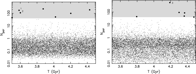
Figure 5: An estimate of the number of comets $N_{\rm par}$ injected into the tidally active zone as a consequence of a stellar encounter (see Eqs. (1) and (2) in Fouchard et al., 2017b): (i) left panel for V1 simulations, (ii) right panel for V2 simulations. Only the values in the last Gyr of the simulations are shown. The strong encounters with $N_{\rm par}\gtrsim 40$ in the gray box are highlighted by large symbols. Details on the comet showers associated with the encounters labeled 1, 2 and 3 are shown in Fig. 10. Most of the stellar encounters constitute a background with $N_{\rm par}\lesssim 2-3$.

For sake of illustration, we find it useful to fold the multi-dimensional information on the stellar encounters, such as their mass, encounter velocity, and the closest approach, into a single-parameter proxy. To that end we use $N_{\rm par}$ defined in Fouchard et al. (2017b) (their Eqs. (1) and (2)). According to this source, $N_{\rm par}$ approximates the number of comets injected into the observable region, and thus shows the importance of a given encounter. We note that $N_{\rm par}$ is similar to a simpler $g$ parameter used in Feng & Bailer-Jones (2015). The difference between the two parameters occurs primarily for high-velocity encounters with low-mass stars. However, since we use $N_{\rm par}$ only as an auxiliary parameter to identify particularly important encounters, these differences are not important. The real importance of the encounter is further studied in Sec. 4 by tracing truly detectable comets in our model.

Figure 5 shows $N_{\rm par}$ values in our single realizations of the V1 and V2 encounter series in the last Gyr of the simulation. Most of the values are $\lesssim 2-3$ and those constitute a background signal. Occasionally, a star passes close enough to surpass this background. The values are slightly more spread in the V2 model because of the considered range of stellar masses. The highest values of $N_{\rm par}$ range between $100$ and $\simeq 550$ in our simulations. Most often, these correspond to subsolar-mass stars passing very close to the Solar system and having small encounter velocities. Only one of these cases, labeled 2 on the left panel of Fig. 5, corresponds to the encounter of a $9$ M_⊙ giant star. We found that the encounters with $N_{\rm par}\gtrsim 40$ (red symbols) produce observable comet showers in our simulations (Sec. 4).

The combined frequency, over all stellar types, of encounters within $1$ pc of the Sun is $\simeq 11$ per Myr. This value seems realistic, even slightly smaller than preliminarily inferred from the Gaia data ($19.7\pm 2.2$ per Myr, Bailer-Jones et al., 2018). Obviously, this flux is dominated by encounters with the lowest-mass dwarfs. The closest generated approaches to the Sun over the $4.5$ Gyr time span were $\simeq 1700$ au. These anomalous encounters penetrate not only the outer, but also the inner, parts of the Oort cloud. However, because the cumulative number of stellar encounters with perihelion smaller than $q_{\star}$ scales as $\propto q_{\star}^{2}$, most of the encounters are much more distant. For instance, their number with $q_{\star}\lesssim 40000$ au is only $\simeq 4$% of the total. It is also interesting to note that these statistics fit the parameters of the closest known stellar approach within the $\pm 10$ Myr interval of time from the present: the dwarf star Gliese 710 is predicted to approach within 10000–20000 au of the Sun about $1.3$ Myr from now (90% confidence interval for distance, e.g., Berski & Dybczyński, 2016; Bailer-Jones, 2018; Bailer-Jones et al., 2018).

Having prepared a look-up table of the initial conditions of stars at the $1$ pc sphere about the Solar system, the effect of stellar encounters was incorporated in our simulations by adding the stars as new massive bodies into the integrations. Because some of the stars may spend up to a few hundred thousand years within $1$ pc of the Sun, at moments the simulation may account for several passing stars. The stars were followed throughout their encounters until they again reached a distance of $1$ pc from the Sun.

3.5 Comet production runs

The observational information about LPCs, summarized in Sec. 2, is based on data collected over the past two centuries (although more than 80% of them are even more recent, and represent discoveries over the past two to three decades only). Ideally, one would wish to compare this data set to modeled comets during a comparably short interval of time. For this to work, however, one would need to include many more planetesimals in our simulations ($\simeq 10^{12}-10^{13}$ instead of $10^{6}$; Sec. 4). This is obviously impossible for computational reasons.

In this situation, we need to trade the smaller number of integrated planetesimals for a longer interval of time over which data are collected (also see Nesvorný et al., 2017, where a similar approach was used). To compensate for the “missing” six to seven orders of magnitude, we need a time interval of at least several tens of Myr. In fact, to have enough statistics, we used the last Gyr in our simulations for this purpose. We find this method adequate, because the comet flux within this interval of time is approximately steady (see, e.g., Figs. 9 and 11). In particular, the very slow decline due to late erosion of the Oort cloud represents an effect of only $\simeq 10-15$% (most of the population dynamics of the Oort cloud is completed by $0.5-1$ Gyr after the beginning; e.g., Dones et al., 2004). As a result, the underlying assumption of a steady state of our model is only very weakly violated. Following methods in Fouchard et al. (2017b) and Fouchard et al. (2017a), we only discard periods adjacent to the strongest comet showers (roughly indicated by encounters having $N_{\rm par}\geq 40$; Fig. 5). Collectively, these cover only about $\simeq 20-30$ Myr from the target Gyr interval of time. This is because our analysis of the comet showers in Sec. 4 indicates that their signal fades away within $2-5$ Myr (the analysis in Bailer-Jones (2018) or Bailer-Jones et al. (2018) showed no stellar encounter within the past $\simeq 10$ Myr that could produce a noticeable comet shower).

Following these considerations, we modified the output from our numerical code between the epochs $3.5$ Gyr and $4.5$ Gyr since the beginning (the last Gyr). We monitored the heliocentric distances $r$ of all particles in our simulations. When, for a given particle, $r$ became smaller than 20 au, we followed its evolution and output the planetary and particle state vectors near its perihelion. Because we focus on LPCs in this paper, the output was performed only when the heliocentric semimajor axis satisfied $a\geq 35$ au (i.e., orbital period longer than $\approx 200$ yr). After completing the primary simulation, we used these data specific to LPCs in the last Gyr to compute the particles’ original orbits before they entered the planetary region. In particular, we performed a sequence of short integrations backward in time from each of the data files and followed the orbit until it reached a heliocentric distance of $250$ au. If the motion reached aphelion before this limit, we used the aphelion state vectors. The dynamical state of the comet was then transformed into the Solar system barycentric frame and the barycentric orbital elements were computed. These are to be compared with the data outlined in Sec. 2. Note that we aligned the 250 au limit with the practice used in the Królikowska et al. catalogs (e.g., Królikowska et al., 2014; Królikowska, 2014; Królikowska & Dybczyński, 2017). The original orbits in MWC08 were computed at a smaller heliocentric distance, but the difference is insignificant.

With the parameters described above, we have full control of the LPC orbital evolution when their perihelia decrease below $20$ au. The choice of this limit resulted from a compromise between several factors. First, it allows us to learn about the orbital evolution even before the comet becomes observable with current surveys (heliocentric distances $\lesssim 10$ au; Sec. 2). Second, it also allows us to theoretically characterize a putative population of LPCs with perihelia between the orbits of Saturn and Uranus. This is interesting because this population may be in reach of forthcoming surveys (note that today’s catalogs contain only four well-observed long-period comets with perihelia beyond Saturn’s semi-major axis of $9.54$ au, with C/2003 A2 (Gleason) ($q\simeq 11.43$ au) being the record holder). Both reasons may motivate us to push the limit even further than $20$ au, but this is problematic at the moment. The population of LPCs steeply increases beyond the perihelion limit of $\simeq 15$ au (see Figs. 12 and 14). Therefore, extending the target zone where comets are being monitored towards the orbit of Neptune (i.e., $30$ au) would (i) produce increasing demands on disk storage, and (ii) slow down the simulations.

3.6 Fading problem for LPCs

Oort (1950) noted that the observed energy distribution of LPCs, which is sharply peaked for $1/a\leq 10^{-4}$ au^-1 (e.g., Fig. 3), is only compatible with model predictions if comets are allowed to remain observable only for a certain number of returns to the inner Solar system. In particular, Oort postulated an average disruption probability of $1.4$% per perihelion passage. But even with this assumption, he was unable to explain the sharp concentration of comets on nearly parabolic orbits. Therefore he assumed that most LPCs (some 80%) are overly active when first arriving in the observable region with small perihelion distances and, therefore, exhaust most of their volatiles that feed the observable comae. When the comets arrive again, they are much fainter and supposedly escape detection. Whether they actually do arrive again, or disrupt (e.g., Levison et al., 2002), is not really relevant to our work. Both constitute what is called the comets’ fading.

Comets are followed in our simulations as unbreakable point particles and may suffer elimination only for dynamical reasons. Because it would be inconvenient to implement the physical lifetime (fading) effects in the numerical simulation of the orbital evolution, we save it for post-processing of the results. This is possible because we have information about the returns of the given comet before it was dynamically eliminated (obviously, only within the target heliocentric region of $20$ au). Cometary fading may be approached as a physical process with all its complexity. This is, however, quite beyond the scope of this paper. Rather, we shall adopt a simple, empirical description of the fading process primarily as a function of the number of returns to the Solar system. A very nice overview of possible choices is given in Sec. 5.5 of Wiegert & Tremaine (1999).

We first tried the simplest possible choice, namely to allow a certain number of perihelion ($q$) returns below a $q$ limit $N_{\rm p}(q)$: this option was used by Nesvorný et al. (2017) for short-period comets with a choice $q=2.5$ au. However, we found that this provides unsuitable results for LPCs, even when changing the $q$ limit. In particular, the ratio of the number of new comets in the Oort peak to the number of returning comets was never well satisfied (this is in agreement with results in Wiegert & Tremaine, 1999). This failure is because such a simple fading law does not fit Oort’s original suggestion that LPCs fade more at their first appearance, and much less later on. One could try ad hoc assumptions about different fading probabilities at different returns. At this point it is actually easier to assume some simple smooth function of the return number. This parametrization was introduced by Whipple (1962) and successfully used by Wiegert & Tremaine (1999). For those reasons, we shall adopt the same approach here.

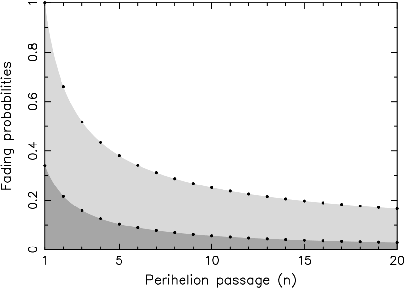
Figure 6: An example of a one-parameter fading law used in our analysis: a power-law probability $\Phi_{n}=n^{-\kappa}$ that a dynamically new comet survives fading for at least $n$ perihelion passages ($n=1$ means its first appearance; see Whipple, 1962; Wiegert & Tremaine, 1999). The upper curve, enclosing the light gray area, shows $\Phi_{n}$ for $\kappa=0.6$ ($\Phi_{1}=1$ implies the comet has been observed). The bottom curve, enclosing the dark gray area, shows the conditional probability $\psi_{n}=1-(\frac{n}{n+1})^{k}$ that a comet which survived $n$ perihelion passages will fade before returning for the $(n+1)$th time.

Whipple (1962) assumed the probability $\Phi_{n}$ for a comet to survive at least $n$ perihelion returns is a simple power-law function: $\Phi_{n}=n^{-\kappa}$, where $\kappa$ is a constant. Both Whipple (1962) and Wiegert & Tremaine (1999) found that $\kappa\simeq 0.6$ provides a good ratio between new and returning LPCs. Figure 6 shows the properties of this choice. We note that some 35% of comets survive only one return and some 60% of comets survive only 5 returns. Beyond that, however, the survivability significantly improves, nearly as if there were two categories of objects: some which die very quickly and some which have very good chances of survival even after many returns. This is the reason for the success of the empirical fading law suggested by Whipple. At the same time, one should admit the limitations of this single-parameter law. Its applicability up to now perhaps means that the comets (i) are observed in a still rather limited region of perihelion distances (note that Wiegert & Tremaine (1999) limited their study to $q<2.5$ au), and (ii) are mostly of a typical size $D$. In principle, the fading must depend on both $q$ and $D$, such that larger comets, and those passing at larger perihelia, should live significantly longer. Some aspects of the size dependence in cometary fading have been quantitatively documented, for instance, for long-period comets with $q<0.5$ au by Bortle (1991) and LPCs with $q<1$ au by Sekanina (2019) (also see discussion in Whipple, 1992). More, and especially well understood, observations will be needed to test the complex parameter dependence of cometary fading. In this paper, we stick with the original simple formulation of Whipple (1962).

3.7 Features not included in our model

Even though we made efforts to present a complete and consistent model for the origin and evolution of LPCs, we neglect several important elements. Here we briefly recall these caveats which will need to be considered in future work.

Effects of the solar birth cluster.– In all likelihood, the Solar system was initially formed within an embedded cluster of stars (see the reviews by Adams, 2010; Pfalzner et al., 2015). Various constraints imply that this birth environment contained hundreds to perhaps a few thousand stars, all located within a few parsec zone. Depending on the cluster parameters, a typical solar analog could have left its natal cluster in a couple of tens of Myr. Before reaching a more friendly environment characterized by the current galactic tidal field and the current frequency of stellar encounters (both outlined above), the early Solar system thus experienced much more fierce conditions.

In terms of small body deposition in the trans-Neptunian zone, most studies focused on two aspects: (i) formation of a fossilized inner Oort cloud, possibly extending inward to a few hundred au from the Sun, and (ii) implantation vs. erosion of the classical Oort cloud. The first line of investigation was motivated by the discovery of a population of extremely detached trans-Neptunian objects, such as Sedna ($q\simeq 76$ au). Indeed, various simulations (see, e.g., Fernández & Brunini, 2000; Brasser et al., 2006; Kaib & Quinn, 2008; Brasser et al., 2012) have shown that stellar encounters at very small distances, typical in the initial phases of the cluster evolution, allow the Oort cloud to extend inward enough to comfortably explain the existence of Sedna and similar bodies. This structure would be unaffected by currently acting galactic tides and thus would remain a fossil relic of the natal stage of the Solar system. It would not contribute significantly to the currently observable population of LPCs. It may become a relevant source of a population of LPCs with more distant perihelia, beyond the orbit of Saturn, if observed in the future. However, some studies suggest that the fossilized inner extension of the Oort cloud may actually be depleted in small bodies (diameters less than $\simeq 4$ km). This is because gas drag in the primordial solar nebula might have prevented transport of such small bodies to this source zone (e.g., Brasser et al., 2007).

As for the second aspect, survival of comets in the classical zone of the Oort cloud, the results depend on cluster parameters and details of the modeling. Levison et al. (2010), assuming very low-mass clusters, showed that the Oort cloud may capture extra-solar planetesimals quite efficiently. It was not clear, though, whether the same model could emplace the right number of objects into the fossilized inner zone of the Oort cloud and thus explain the Sednoid population. Other studies of more massive clusters generally did not reach the same level of sophistication as the work of Levison et al. The investigations of more massive clusters focus on the disruptive role of stellar encounters with the classical Oort cloud (e.g., Kaib & Quinn, 2008; Nordlander et al., 2017)

We neglect the effects of the birth cluster on the formation of the Oort cloud. Formation of the Oort cloud might have been a two-stage process (also see Brasser et al., 2008; Brasser & Morbidelli, 2013; Nordlander et al., 2017). The first phase involved dynamics in the birth cluster. This might have stored bodies in the fossilized inner Oort cloud and left some population of comets in the classical Oort cloud zone. Assuming that the Sun left the cluster prior to the planetary instability, our model describes what happened later on.

Solar migration in the Galaxy.– Another badly constrained issue of Oort cloud formation has to do with the solar orbit in the Galaxy. This is because the Oort cloud was principally built some $4$ Gyr ago (e.g., Dones et al., 2004). However, there is no exact constraint on the Sun’s location in the Galaxy at that epoch. Our model assumes the current orbit at all times, but very likely the Sun performed a more complicated journey in our Galaxy throughout its history. The most interesting aspect is its possible radial migration (see, e.g., Roškar et al., 2008; Martínez-Barbosa et al., 2015; Frankel et al., 2018). Migration would have directly affected both galactic tide parameters and the frequency of stellar encounters.

Several groups have studied Oort cloud formation in different galactic environments (e.g., Brasser et al., 2010; Kaib et al., 2011; Martínez-Barbosa et al., 2017; Hanse et al., 2018), indicating that if the Sun was at a small galactocentric distance during its early history, the effects would be somewhat similar to the birth cluster. In particular, stronger tides and fiercer stellar encounters would lead to the formation of the Oort cloud closer to the Sun, extending its innermost zone perhaps near the Sednoid region. For that to work, one should prefer models in which the Sun spent its infancy at a rather small distance from the center of the Galaxy. Additionally, a later solar excursion into this zone may cause stronger erosion of the outer Oort cloud region which currently provides observable LPCs. These accelerated losses may be somewhat compensated by transfer from the inner regions of the Oort cloud (e.g., Kaib et al., 2011).

With this perspective, we should consider our model a baseline before we consider more complex possibilities. If future observations of large-perihelion LPCs indicate a large mismatch with our predictions, more careful studies involving models of the birth cluster and/or solar radial migration in the Galaxy will be needed.

Massive perturbers in the outer Solar system (planet 9).– Several groups of researchers have recently suggested the existence of a massive ($\approx 5$–20 Earth mass) body (planet 9) roaming in the region beyond the classical Kuiper belt (e.g., Trujillo & Sheppard, 2014; Batygin & Brown, 2016a; Batygin et al., 2019). This body was needed, according to them, to explain the non-uniform distributions of secular angles (node and perihelion longitudes) of about a dozen trans-Neptunian objects with extremely distant orbits (i.e., $a>150$ au, $q>35$ au). Planet 9 may also act as a perturber that tilted the giant planets’ invariant plane from the solar spin direction (e.g., Bailey et al., 2016; Lai, 2016; Gomes et al., 2017) and produce high-inclination, large-semimajor axis Centaurs (e.g., Gomes et al., 2015; Batygin & Brown, 2016b; Batygin et al., 2019). While intriguing in many respects, the hypothesis of the distant planet 9 is still debated. For instance, analysis of observations by the Outer Solar System Origins Survey (OSSOS), currently the most prolific survey of the trans-Neptunian region, are still compatible with a uniform distribution of orbital angles of distant objects when biases are properly accounted for (e.g., Shankman et al., 2017; Bannister et al., 2018), although the originators of the planet 9 hypothesis find that the clustering is highly significant (Brown & Batygin, 2019). The solar tilt may have been produced in an earlier phase of Solar system evolution (e.g., Heller, 1993; Thies et al., 2005; Batygin et al., 2019), and in spite of search campaigns, planet 9 still escapes direct detection.

As for the relation to cometary studies, Nesvorný et al. (2017) examined the role of planet 9 with the parameters originally suggested by Batygin & Brown (2016a) for orbital and population characteristics of short-period comets. They found that existence of planet 9 on this orbit, with a mass of 15 Earth masses, makes it difficult to explain the tight inclination distribution of Jupiter-family comets. This is because planet 9 directly affects the properties of planetesimals in the scattered disk, which acts as an immediate source for these comets. As to the Halley-type comets, which are generally thought to originate for the most part from the Oort cloud, Nesvorný et al. (2017) did not find any improvements to the model. In fact, when planet 9 was taken into account, the match of the orbital elements of Halley-type comets was not as good. Also, perturbations from planet 9 were not found to significantly increase the flux of Halley-type comets when compared to the model where only the galactic forces were taken into account. Since LPCs originate from the Oort cloud, it is hard to imagine that planet 9 would significantly improve the modeling of the currently observed population of these comets. Future work may test the effect of planet 9 on a putative population of LPCs with distant perihelia.

With this experience, and because the current situation of planet 9 is rather confused, we opted not to include it in the present study.

Nongravitational accelerations in cometary dynamics.– The original orbital elements inferred for comets, in particular their original semimajor axes, depend on their levels of activity. So whenever enough astrometric observations are available, orbit fitters typically include nongravitational effects. This procedure was started and tested by the founders of MWC08 (e.g., Marsden et al., 1973; Marsden & Sekanina, 1973; Marsden et al., 1978), and later on verified and incorporated into the Królikowska et al. catalogs (e.g., Dybczyński & Królikowska, 2011; Królikowska & Dybczyński, 2013; Królikowska et al., 2014). As a rule of thumb, these authors found that many apparently hyperbolic solutions among the original orbits are moved to the category of very weakly-bound, but elliptical solutions (often in the Oort peak). This is a very interesting result, pointing to the importance of nongravitational accelerations in cometary dynamics.

Wiegert & Tremaine (1999) (see their Fig. 20) also noted that the predicted distribution of the original semimajor axis changed when nongravitational effects were included. They found that (i) the dynamical effects correlate with the fading law, and (ii) simple parametrization of the nongravitational effects worsens agreement with the observations for comets on returning orbits with small semimajor axes (perhaps because modeling of the recoil effects due to comet activity is too simplistic). As a result, while admitting their importance, we also neglect nongravitational effects in our work.

4 Results

4.1 Properties of the Oort cloud

First, we take a brief look at the Oort cloud structure at the end of our simulations, namely at $4.5$ Gyr. Since all our runs provide very similar results, we use C1V1 as an example. We also note that the situation becomes nearly stationary during the last Gyr, so our analysis is representative of any moment, except for rare comet showers, during that interval of time. As mentioned above, the Oort cloud population declined in the C1V1 run by only $\simeq 12$% from $3.5$ Gyr to $4.5$ Gyr.

Figure 7 shows the orbits of slightly more than $51000$ particles remaining in the C1V1 simulation at $4.5$ Gyr. The innermost structures, with $a\lesssim 1000$ au, are of lesser importance for our current work. They include the dynamically hot classical Kuiper belt, resonant populations (including Plutinos), and objects stored in the scattering disk, most with $q<35$ au. Only objects interacting with high-order exterior resonances with Neptune may become detached beyond this perihelion distance by processes described in Nesvorný et al. (2016) and Kaib & Sheppard (2016). The scattering population is relevant to our study by constituting a pathway which objects take to reach larger heliocentric distances. There is also a population of a few objects with $q<30$ au and $a<1000$ au seen in Fig. 7. One would classify them as an extreme Centaur population, which will further evolve toward short-period comets. Some of these objects may also be considered in our analysis below as returning long-period comets (unless they already performed so many returns that they would be classified as faded objects). Large surviving comets in this region continue their evolution towards the class of Halley-type comets (e.g., Nesvorný et al., 2017).

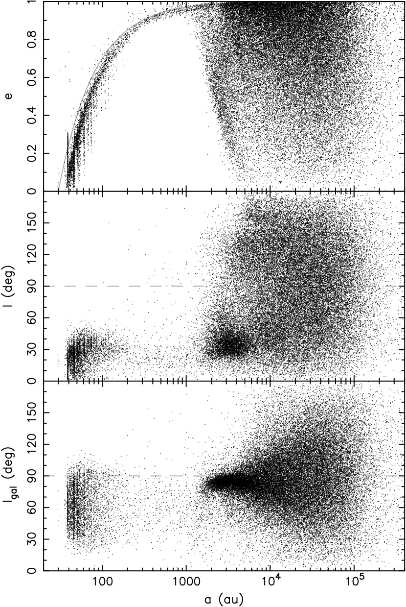
Figure 7: Orbits of all $\simeq 51000$ particles remaining in the simulation C1V1 at $4.5$ Gyr: (i) semimajor axis vs. eccentricity (top), (ii) semimajor axis vs. inclination with respect to the ecliptic plane (middle), and (iii) semimajor axis vs. inclination with respect to the galactic plane (bottom). The gray line at the top denotes $q=30$ au (Neptune’s heliocentric distance); the dashed lines in the middle and bottom panels denote polar orbits with $i=90^{\circ}$ (or $i_{\rm gal}=90^{\circ}$). The scattering disk (active, detached and the outer resonant populations) contains some $4600$ particles up to semimajor axis $a\simeq 1500$ au (with a majority of $\simeq 85$% with $a<200$ au. The inner and outer parts of the Oort cloud contain $\simeq 21500$ and $\simeq 24300$ particles with $a<15000$ au and $a>15000$ au, respectively; 15000 au approximately represents the division between the non-isotropic and isotropic portions of the populations.

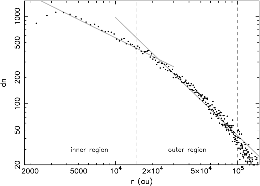
Figure 8: Radial distribution of particles remaining in the simulation C1V1 at $4.5$ Gyr: the symbols give the number of particles $dn$ in bins $dr=500$ au (for the distribution law $dn=n(r)\,dr$). The dashed vertical lines roughly delimit the inner and outer parts of the cloud, where the power-law approximations $n(r)\propto r^{-\alpha}$ have different exponents: (i) $\alpha\simeq 0.72$ in the inner part, and (ii) $\alpha\simeq 1.35$ in the outer part. Below $r\simeq 2000$ au the population abruptly drops (also see Fig. 7).

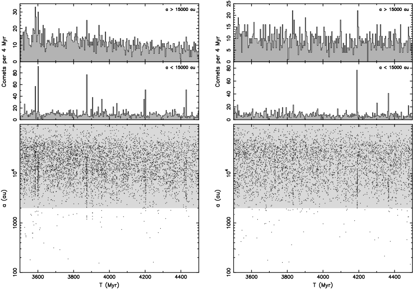
Figure 9: Orbits of comets at their first appearances inside the heliocentric target zone $r\leq 20$ au: left panels for the C1V1 simulation, right panels for the C1V2 simulation. The abscissa is time in the last Gyr of the simulations. The bottom panels show the original semimajor axes $a$ of the orbits (the gray zone approximately delimits the heliocentric distance range of the Oort cloud). The upper panels show the number of new comets in $4$ Myr bins. We separate cases originating from the outer/inner parts of the Oort cloud (with $a>15000$ au and $a<15000$ au, respectively). Cometary showers, associated with particularly strong stellar encounters (Fig. 5), are clearly seen coming from the inner Oort cloud, while their signal is absent in the outer Oort cloud.

Further on, at $a\gtrsim 1500$ au, we reach the realm of the Oort cloud. The lower two panels in Fig. 7, showing the inclination with respect to the ecliptic (middle) and galactic (bottom) planes, best illustrate the two distinct regions, the inner and outer Oort clouds. The anisotropic nature of the inner part, from semimajor axes $\simeq 1500$ au to $\simeq 15000$ au, is readily explained by the orbital evolution due to galactic tides (e.g., Higuchi et al., 2007; Higuchi & Kokubo, 2015; Fouchard et al., 2017b). In this region the tides are too weak, such that orbits pulled from the tail of the scattered disk perform less than one cycle of their secular evolution (see, e.g., Fig. 3 in Fouchard et al., 2017b). The slow evolution towards small eccentricity values produces the visible edge of the inner Oort cloud and also implies that inclinations with respect to the galactic plane are strongly concentrated towards $90^{\circ}$, where the secular evolution spends most of the time (e.g., Higuchi et al., 2007). Because the mean inclination of the scattered disk is $\simeq 60^{\circ}$ in this reference frame, the orbits do not overcome the $90^{\circ}$ limit in the quadrupole tidal model. They may scatter over this limit only by occasional tugs due to passing stars. Transformed to the ecliptic frame, this concentration occurs at $\simeq 35^{\circ}$, with a weaker concentration near $\simeq 150^{\circ}$. In the outer part of the Oort cloud, beyond semimajor axes $\simeq 15000$ au, the inclination distribution becomes nearly isotropic in space. Orbits in this region have performed at least several secular cycles due to the tides, helping in their mixing. More importantly, beyond about $\simeq 40000$ au the purely secular model is not justified, because the strength with which orbits are bound to the Sun becomes similar to the tidal effects. The orbits become essentially chaotic (also see Brasser, 2001). Finally, orbital mixing due to the stellar passages becomes a vigorous process in this zone.

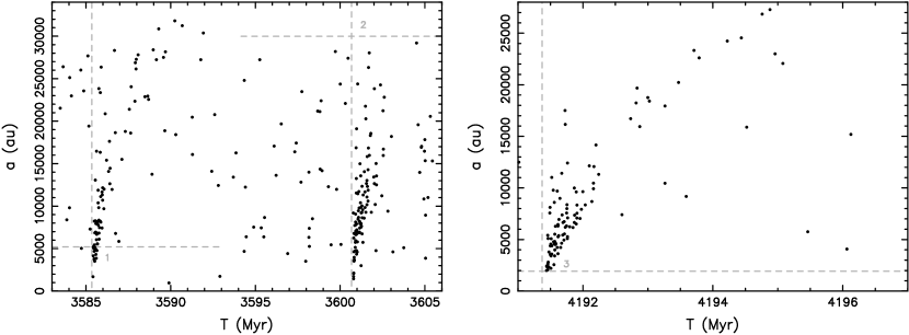
Figure 10: Two examples of comet showers into the heliocentric target zone $r\leq 20$ au (highly time-zoomed data from the bottom panels of Fig. 9). Orbits of comets at their first appearance, with time as abscissa and original semimajor axis as ordinate, for the stellar encounters highlighted by labels 1, 2 and 3 of Fig. 5 are shown. The horizontal dashed lines indicate the smallest distance at which the star encounters the Sun, while the vertical dashed lines indicate the epochs of the closest encounters. Left: Two encounters, fortuitously close in time, from simulation C1V1. The first, labeled 1, represents a star of $0.78$ M_⊙ mass encountering the Solar system with an asymptotic velocity of 24 km s^-1 , while the second, labeled 2, represents a star of $9$ M_⊙ mass encountering the Solar system at $14$ km s^-1. Right: a single encounter in the simulation C1V2 with the largest recorded value $N_{\rm par}\simeq 540$, corresponding to a $0.26$ M_⊙ star encountering the Solar system at $16$ km s^-1 at a minimum distance of $\simeq 1920$ au. The “triangular” shapes of the showers imply that comets from larger-$a$ orbits generally arrive slightly later, as expected.

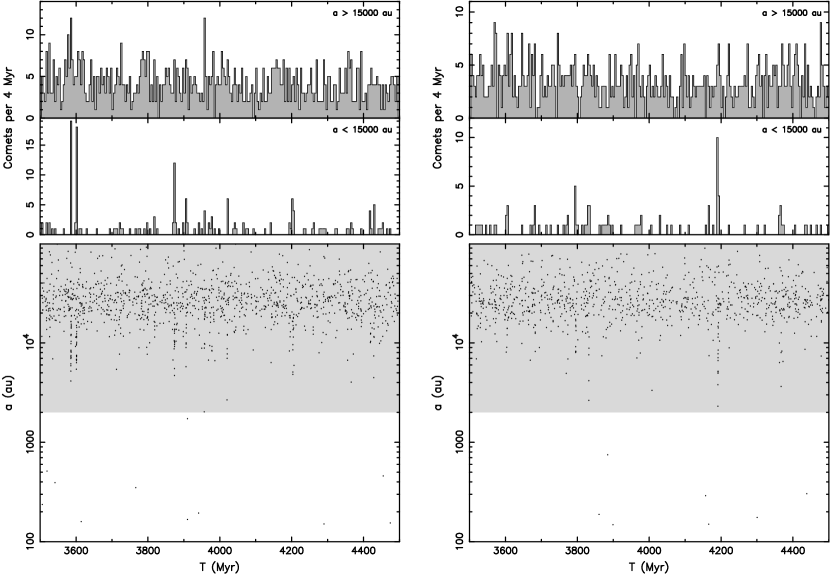
Figure 11: The same as in Fig. 9, but now for the first appearance of comets inside a much more restricted heliocentric target zone $r\leq 5$ au. Now the inner Oort cloud is basically absent as an apparent source of new comets except during strong cometary showers. Most of the flux of new comets now comes from the outer Oort cloud with $a>15000$ au.

Figure 8 shows the radial heliocentric distribution of comets in the Oort cloud at the end of our simulation C1V1. We plot the number of objects $dn$ in uniform radial steps $dr=500$ au. While not exactly a power law, the incremental distribution function $n(r)=dn/dr$ may be in parts approximated with $n(r)\propto r^{-\alpha}$. In the inner cloud, we find $\alpha\simeq 0.72$, while in the outer cloud, we find $\alpha\simeq 1.35$, steepening to a thermalized value of $1.5$ at the very outer edge of the cloud (beyond $\simeq 50000$ au). [Note our $\alpha=1.5$ corresponds to $\alpha=-3.5$ as defined by Duncan et al. (1987)]. The population of the inner region of the cloud is comparable, but actually slightly smaller than, that of the outer region. This is also related to the shallow power-law exponent (inspecting our other simulations, we have $\alpha$ always in the range of $0.68$ to $0.77$ in the inner Oort cloud). The Oort cloud formed in our model therefore has a less populous inner region, if compared to some previous models (often assuming the thermal exponent $1.5$ extending throughout the whole cloud). However, the results here are comparable to several other models such as Dones et al. (2004). Note that the Oort cloud fills in from the outer parts to the inner zone. Therefore, details of the population in the inner cloud depend sensitively on the late deposition of planetesimals in the tail of the scattered disk in the migration scenario. We find that the inner zone starts to fill effectively at $\simeq 250-300$ Myr (compare with Fig. 8 of Dones et al., 2004). This explains why our C1 and C2 models (see Table 1) produce rather comparable results: the assumed timescales $\tau_{1}$ and $\tau_{2}$ are still short, if compared to the inner Oort cloud filling timescale.

4.2 Comets at their first appearance

As discussed by Wiegert & Tremaine (1999, their class V₁), the properties of LPCs at their first appearance in the target zone may be a useful starting point for their analysis as a whole. We start with discussion of the orbital parameters of new comets in the largest target zone monitored during the last Gyr in our simulations, namely the heliocentric sphere of $20$ au (Sec. 3.5). This zone is larger than the currently observable region, but future observations hope to reach this zone. While speaking about new comets here, we point out that we do not know their orbital evolution before appearing in this target zone. In particular, we do not know whether a particular orbit jumped in from a very distant-perihelion state, or whether its perihelion was slowly evolving towards the $20$ au limit.

In Figure 9, the lower panels show the original semimajor axes $a$ of newly-appeared LPCs in the $r\leq 20$ au zone during the last Gyr in the C1 simulations. In the two variants of stellar encounters, V1 and V2, there are about $5500$ and $4350$ data points in the respective runs. Two patterns are seen: (i) randomly distributed data with no strong correlation between time and original semimajor axis, and (ii) occasional sequences of new comets strongly localized in time. The former is a background population, originating from the entire Oort cloud. In each of the two variants, comparable numbers of comets arrive from the inner and outer parts of the Oort cloud, roughly in proportion to their populations (Fig. 8). The second, time-correlated component in the population of new comets constitutes showers after the most important stellar encounters. Their occurrence coincides very well with the events for which $N_{\rm par}\geq 40$ in Fig. 5. Note that cometary orbits in these showers apparently originate only from the inner part of the Oort cloud, for which $a\lesssim 15000$ au. This is again well documented in the upper panels of Fig. 9, where we show the number of comets collected in $4$ Myr wide bins in time. The dominance of the inner Oort cloud in its contribution to the shower periods is well known from previous studies (e.g., Heisler et al., 1987; Heisler, 1990; Fouchard et al., 2011a), though that work often focused on smaller heliocentric target zones. The largest contrast between the number of new comets in the modeled showers and the long-term mean of the background signal is $\simeq 4-5$. This is in accord with results of Fouchard et al. (2011b) and Fouchard et al. (2011a).

Figure 10 provides a zoom of the lower panels in Fig. 9 for three prominent showers: (i) the left panel illustrates the results of the two stellar encounters labeled 1 and 2 in Fig. 5 from the C1V1 simulation, while (ii) the right panel illustrates comets from the strongest stellar encounter, labeled 3 in Fig. 5, from the C1V2 simulation (parameters of the stellar trajectories relative to the Sun are given in the caption). Clearly, comets having smaller-$a$ orbits statistically arrive first, because of their smaller orbital periods. However, because the encounters occur at a random phase of the orbital motion of the comet (i.e., some comets with large semimajor axes are near perihelion), some with larger-$a$ orbits may also arrive nearly instantly. Nevertheless, those which are delayed with respect to the stellar passage must also arrive from very wide orbits. This produces the triangular shape of the region where the shower comets are concentrated. It has been noted in several earlier studies that the strongest showers are not necessarily produced by encounters with the most massive stars. There are very rare and may happen only once or twice in the history of the Solar system (for stars with mass $\gtrsim 10$ M_⊙, say). Statistically more important are very close, and low-velocity, encounters with sub-solar mass stars. These may happen once per $\simeq 100-150$ Myr, on average (e.g., Heisler et al., 1987; Heisler, 1990; Fouchard et al., 2011a).

Figure 11 shows the same information as Fig. 9, but now restricted to the heliocentric target zone $r\leq 5$ au. This range is now compatible with the perihelia of the presently observed comets (Sec. 2). As expected, almost all members in the background population of new comets come only from the outer part of the Oort cloud. With a few outliers, the inner Oort cloud becomes active only during the strongest comet showers (see Hills, 1981; Heisler et al., 1987; Heisler, 1990). This is expected, because tides are efficient enough to fill the phase space region of LPC orbits reaching $q<5$ au (their “loss cone”) only for $a\gtrsim 30000$ au. Comets with $a$ down to about $15000$ au may also contribute, if they creep their perihelia through the planetary zone above the orbit of Saturn and eventually increase their semimajor axes enough by planetary perturbations before the final jump into the observable zone (e.g., Kaib & Quinn, 2009). However, orbits with semimajor axes in the inner Oort cloud undergo changes in perihelion distance in one orbit that are too small, so that Jupiter and Saturn efficiently eliminate them before they can appear with perihelia within Jupiter’s orbit (see also Rickman et al., 2008; Fouchard et al., 2011a, 2014).

Figure 12: Cumulative distribution $N(<q)$ of LPCs’ perihelia $q$ in two different heliocentric target zones: (i) $q\leq 5$ au (left), and (ii) $q\leq 20$ au (right), both in the simulation C1V1 (data during the strongest comet showers with $N_{\rm par}\geq 40$ were eliminated from the distributions shown). The red curves are for comets at their first appearance in the target zone. The gray curves are linear-quadratic fits of the new comet $q$ distributions, namely (i) $N(<q)\propto q+0.09\,q^{2}$ in the left panel, and (ii) $N(<q)\propto q+0.06\,q^{2}$ in the right panel. The latter matches the $N(<q)$ distribution sufficiently well only until $q\simeq 15$ au, beyond which the number of new comets steeply rises. The blue curves show the cumulative distributions $N(<q)$ when all returning comets are included (no physical fading).

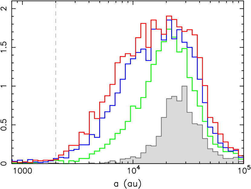
Figure 13: Distribution of semimajor axes of LPCs at their first appearances in heliocentric zones of different radius $r$ in simulation C1V1 (data during the strongest comet showers with $N_{\rm par}\geq 40$ were eliminated from the distributions shown). The gray histogram is for $r\leq 5$ au and roughly corresponds to the currently observed population (see Figs. 1, 3 and 4); this is the “traditional” Oort peak of new comets. The color histograms show the same, but for larger heliocentric target zones: (i) $r\leq 10$ au (green), (ii) $r\leq 15$ au (blue), and (iii) $r\leq 20$ au (red). The ordinate is arbitrarily normalized to unity for the maximum of the $r\leq 5$ au histogram. The total number of new comets in the $r\leq 20/15/10$ au zones is $\simeq 4.5/3.9/2.7$ times larger than the population entering the $r\leq 5$ au zone.

The results discussed above confirm the critical role of the radius $r$ of the target zone around the Sun where new comets are being recorded, especially if crossing the Jupiter-Saturn zone. We repeated our analysis for several choices of $r$. Focusing on the background population of new comets, each time we eliminated comets in the strongest showers (stellar encounters with $N_{\rm par}\geq 40$) from the data. Figure 13 shows the incremental distribution of the original semimajor axes of LPCs as they first arrive in the target zone during the last Gyr of our simulation C1V1 (results for other simulations are very similar). The gray distribution corresponds to the data in Fig. 11, thus $q\leq 5$ au comets. This is the classical Oort peak of nearly parabolic comets seen in the observed population of LPCs (see Fig. 1). When extending the limiting $r$ to larger values (green to red curves in Fig. 13), we note two systematic effects: (i) original orbits with smaller $a$ values start to dominate and the overall distribution of $a$ becomes broader, and (ii) the total population of new comets increases approximately proportionally to $r$. This is because the inner Oort cloud is now able to contribute to the population of new comets (see also Silsbee & Tremaine, 2016; Fouchard et al., 2017a).

We have not yet discussed the distribution of the new comets’ perihelia. This information is shown in Fig. 12 for two heliocentric target zones, $r\leq 5$ au on the left and $r\leq 20$ au on the right. Focusing first on the restricted $5$ au heliocentric zone (left panel), we confirm results from previous studies (e.g. Wiegert & Tremaine, 1999; Fouchard et al., 2017a) that the cumulative perihelion distribution of new comets is very well fitted with a linear term and a small quadratic contribution. Interestingly, if we use the orbits of both new and all returning comets before their dynamical elimination (therefore applying no fading), the perihelion distribution is not changed much (blue curve in the left panel of Fig. 12; therefore, it is to be expected that even when applying some fading law the perihelion distribution would still behave the same). The top two panels in Fig. 15 may offer the explanation: once the orbits happen to decrease their perihelia below Jupiter’s orbit, its value stays approximately constant until elimination. Obviously, a possible caveat of our simulation is the absence of the terrestrial planets. It is yet to be seen whether their gravitational perturbations modify these perihelia distributions.

Extending the heliocentric target zone again to $20$ au, we obtain the results shown in the right panel on Fig. 12. The linear-quadratic trend in the cumulative perihelion distribution of new comets (red curve) continues to about $q\simeq 15$ au. Beyond this point, the population of new comets increases steeply. A similar behavior is also seen in the perihelion distribution of all new and returning comets in this zone (blue curve), though the difference with respect to the statistics of new comets is now a little larger. This is because the returning comets have more space to random-walk their perihelia, especially above the orbit of Saturn.

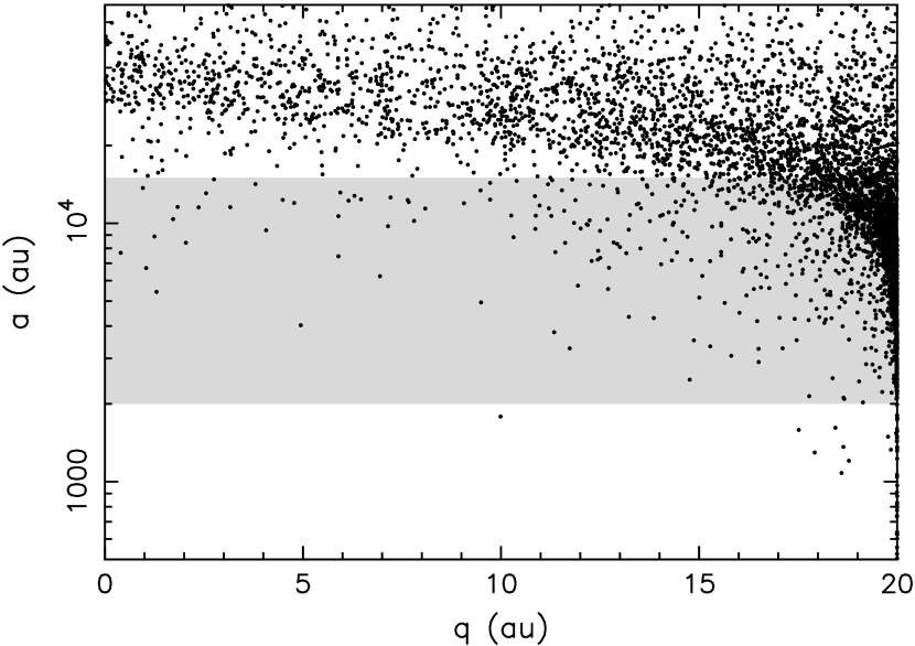
Figure 14: Correlation between the perihelion distance $q$ (abscissa) and the original semimajor axis $a$ (ordinate) for LPCs at their first appearance in the heliocentric target zone $r\leq 20$ au. We used data from the last Gyr of simulation C1V1 used (the signal from the strongest comet showers with $N_{\rm par}\geq 40$ was eliminated from this plot). The gray rectangle shows the approximate location of the inner part of the Oort cloud. At small heliocentric distances, up to $10-12$ au, the apparent source zone of new LPCs is in the outer Oort cloud. Beyond $\simeq 15$ au the inner Oort cloud starts to contribute, and near $20$ au the inner Oort cloud becomes the dominant source zone (also see Figs. 9, 11, 13 and 12).

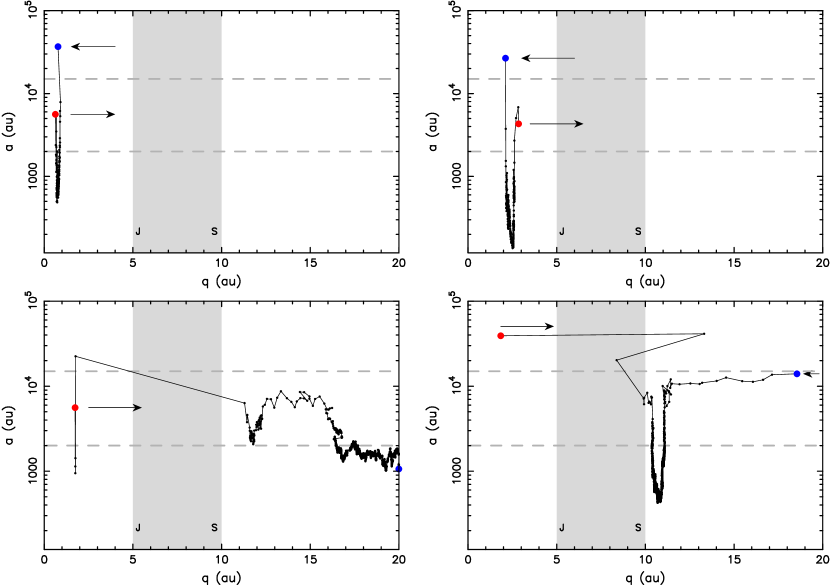
Figure 15: Four examples of LPC orbital evolution in our simulation C1V1: for each return we show the perihelion distance $q$ (abscissa) vs original semimajor axis $a$ (ordinate). Data are collected only when $q\leq 20$ au (the orbital evolution before reaching this limit is not recorded). The first appearance in the $20$ au heliocentric zone is shown by the blue symbol, the last by the red symbol (no physical fading is assumed, so the comet is dynamically eliminated after its last return; arrows indicate the sense in which the orbits are injected or ejected from the monitored zone). Data for the intermediate returns are shown by black symbols and connected by lines to indicate their sequence. The gray rectangle shows the Jupiter-to-Saturn heliocentric zone, and the gray-dashed horizontal lines indicate the inner Oort cloud. The upper panels are examples of “jumpers”, LPCs that appear in the currently observable $q\lesssim 5$ au zone without having a prior perihelion evolution closer than $20$ au. The bottom panels are examples of “creepers”, LPCs that had many tens of returns in the ice-giant region above Saturn’s orbit before first appearing in the currently observable $q\lesssim 5$ au zone. Note that all these cases appear to be injected into the $q\lesssim 5$ au zone from the outer Oort cloud (i.e., initially with $a>15000$ au).

The rapid increase in the population of new comets beyond about $15$ au is intriguing. To shed more light on this topic, we plot the correlation between perihelia $q$ and original semimajor axes $a$ of new comets using our outermost target zone of $r\leq 20$ au in Fig. 14. Orbits with $a\gtrsim 30000$ au populate all perihelion distances about equally. This is because the magnitude of the perihelion change $\Delta q$ in one orbit, roughly expressed as $\Delta q\propto\sqrt{q}\,a^{7/2}$ for both tidal effects and stellar perturbations (e.g., Rickman et al., 2008; Rickman, 2010), is large enough to decrease the perihelion distance to arbitrarily small values from $q\geq 30$ au initial orbits. If the orientation of the comet’s orbit is in a certain range, the outer Oort cloud thus may contribute by injecting comets to perihelia below Jupiter’s orbit. As the target zone slightly increases, the outer Oort cloud may contribute from slightly lower-$a$ initial orbits and this produces the small quadratic term in the cumulative distributions in Fig. 12. Beyond $q\simeq 15$ au, the population of the inner Oort cloud also contributes. This time a variety of orbital evolutions before entering the target zone are possible. Either a direct jump or, more often, a gradual decrease of perihelion in small steps (creeping) can occur. Neptune, with its smaller mass than Jupiter or Saturn, is not a big obstacle to this process. In this way, a significant number of comets may gradually evolve to perihelia between 15 and 20 au from the inner Oort cloud. This also implies that these distant-perihelia comets have orbits that are not isotropic. Instead, their inclination distribution approximately reflects the source zone, with an overabundance of orbits with $\simeq 40^{\circ}$ inclination to the ecliptic plane.

In order to illustrate some of the principles mentioned above, and bridge into the next section, in Fig. 15 we present a few examples of orbital evolutions from our simulations (no physical fading was included in these illustrations). The upper two panels show a typical jumper evolution: the original semimajor axis in the outer part of the Oort cloud allows a very large change in perihelion distance, landing at $q\simeq 1$ au or $2$ au. Next, the perihelion distance stays approximately constant, while the semimajor axis drifts. This is the classical characteristic dynamics of the returning population of LPCs, as we discuss in the next section. The two bottom panels describe what has been characterized as creeping evolution (e.g., Kaib & Quinn, 2009; Fouchard et al., 2014). Thinking about currently observable comets, both cases shown in the lower panels enter the $q<5$ au zone from the outer Oort cloud (at least in terms of the original semimajor axis). Yet, they experienced a significant perihelion evolution in the Saturn–Uranus zone. At least the bottom left case might have initially walked in from the inner Oort cloud. Prerequisite to this evolution is a sufficient increase in semimajor axis before jumping into the observable zone (to perform the necessary $\Delta q$ relative to its instantaneous value). Related to our previous discussion of the data shown in Fig. 14, both of the orbits in the lower panel enter the $20$ au target zone as new comets with very large perihelion values ($\geq 18$ au), both representative of the inner Oort cloud source.

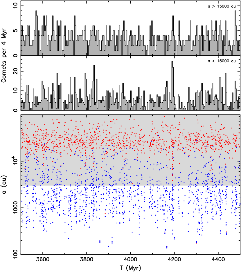
Figure 16: The same as in the right panels of Fig. 11, but now new comets in the heliocentric target zone $r\leq 5$ au are also allowed to contribute by their subsequent returns (up to four of them). Data from the last Gyr of the simulation C1V2 are used here. The bottom panel shows the original semimajor axis $a$, with red symbols for new comets and blue symbols for returning comets. The upper panels show the number of comets in 4 Myr bins. We separate cases originating in the outer/inner parts of the Oort cloud (with $a>15000$ au and $a<15000$ au), respectively.

4.3 Returning population of comets

We now briefly demonstrate the effect of subsequent returns of LPCs. Previous experience showed (see, e.g., Sec. 3.6) that many observed LPCs do not survive a large number of returns. So, while in our simulations some particles underwent hundreds of perihelion passages before experiencing dynamical elimination, our preferred fading law allows only a few returns before the typical comet experiences physical elimination.

For the sake of illustration, we thus extended the data about new comets in the C1V2 simulation from Fig. 11 (right panels) by allowing up to an additional four returns. We also maintain $5$ au as the radius of the target zone, in which these comets are assumed to be observed. The result is shown in Fig. 16: the bottom part shows the original semimajor axes of recorded comets, with red symbols for their first appearances and blue symbols for their subsequent returns. We note the following.

First, while occasionally the returning orbits have semimajor axes in the outer Oort cloud, most often they are shifted to much smaller values. These changes in semimajor axis are produced by planetary perturbations. New comets, after first visiting the inner Solar system, typically suffer a change in the inverse of their original semimajor axis of order $\delta(1/a)\simeq(0.5-1)\times 10^{-3}$ au^-1 due to interactions with the giant planets (e.g., Everhart, 1968; Rickman, 2010). About half of them are lost to interstellar space, while the other half is stabilized to much more strongly bound orbits out of the Oort peak. They populate the hump of returning orbits with semimajor axis values between a few hundred and a few thousand au seen in the data compiled by MWC08 (Fig. 1). This is satisfactorily indicated by the set of blue symbols in Fig. 16.

The second observation concerns the significance of comet showers. The top panel indicates that their visibility is further diminished if the population of returning comets is added. In the case of new comets, those with $a\leq 15000$ au were basically only shower members (Fig. 11); now the returning component from the outer Oort cloud feeds the background signal in this category of orbits. Additionally, even the shower signal may get spread over a longer interval of time when returns of their members are included in the data. This is because the initial shower orbits may have orbital periods ranging from a little less than $100$ kyr to several Myr and this defocuses the narrow signal of the shower.

Finally, data in the top panels of Fig. 16 indicate that the long-term mean flux of LPCs in this simulation, new and returning comets with up to 4 returns, is $\simeq 1.5-2$ Myr^-1 from the initially integrated million particles in the source zone. In the next Section we shall elaborate on the expected flux. We shall also use the calibration of the planetesimal disk population to express these data in terms of the mean size of the observed long-period comets in our model.

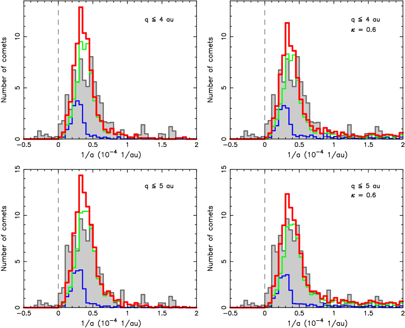
Figure 17: Comparison between data (gray histogram) and simulations for LPCs on nearly parabolic orbits: incremental distribution of the inverse values $1/a$ of the original semimajor axis. The top panels are comets with $q\leq 4$ au, while the bottom panels are comets with $q\leq 5$ au. The panels on the left use only simulated new comets in the target zone, while the panels on the right also include returning comets with Whipple’s power-law parametrization of the fading law and exponent $\kappa=0.6$ (Section 3.6). The red histogram is the total population predicted by our C1V1 simulation normalized to the same number of comets as the data ($78$ in the upper panels, and $95$ in the bottom panels). The blue histogram indicates the jumper component and the green histogram shows the creeper component in all simulated comets.

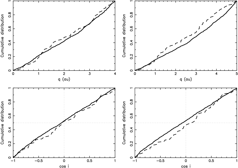
Figure 18: Comparison between data (dashed curve) and simulations (solid curve) for LPCs on nearly parabolic orbits: cumulative distribution of the perihelion distance $q$ (top panels) and cosine of inclination $\cos i$ with respect to the ecliptic plane (bottom panels). Panels on the left are for a population of LPCs with perihelia $q\leq 4$ au, while panels on the right are for a population of LPCs with perihelia $q\leq 5$ au. Simulations use our C1V1 run and also include returning comets with Whipple’s power-law parametrization of the fading law and exponent $\kappa=0.6$. Both data and simulated orbits assume $1/a\leq 2\times 10^{-4}$ au^-1, i.e., $a>5000$ au (Fig. 17) to correspond to the nearly parabolic class.

4.4 Comparison with observations

We now compare our simulations with the available data summarized in Sec. 2. We first consider comets on nearly parabolic orbits, i.e., those in the traditional Oort peak, and then continue with discussion of all LPCs.

4.4.1 Nearly parabolic comets

Our reference data set for this class of orbits comes from the Królikowska et al. catalogs described in Section 2.2. We selected $134$ high-quality orbital solutions with uncertainty in $1/a$ smaller than $10^{-5}$ au^-1. However, the perihelion distribution of this sample includes few orbits beyond $\simeq 6$ au, or even less (Fig. 4). Therefore, in order to minimize this bias, we restrict ourselves to a sub-sample corresponding to a smaller perihelion cutoff. To see the sensitivity to the cutoff limit, we chose two values: (i) $q\leq 4$ au, and (ii) $q\leq 5$ au, the first being a more conservative choice. In what follows, we keep using data from our simulation C1V1, but we checked that the other simulations produce basically identical results. When handling the orbits from the last Gyr of the simulations (Section 3.5), we avoided the $4$ Myr intervals following the strongest stellar encounters. This prevents confusion with periods of cometary showers.

Figure 17 shows data for the distribution of the original semimajor axis using the appropriate binding energy $1/a$ instead of $a$. The upper panels are for the heliocentric target zone of $r=4$ au, while the bottom panels assume $r=5$ au. The cometary orbits contributing to the Oort peak are often approximated with a population of new comets only (e.g., Fouchard et al., 2017a). Therefore, the left panels on Fig. 17 use only our simulated LPCs when they first appear in the target zone. However, Fig. 16 showed that orbits of some returning comets may also occasionally contribute to the population of nearly parabolic orbits. For that reason, in the right panels of Fig. 17 we show results from a more complete, and also more realistic, model where returning comets were added. We used the Whipple fading power-law model with exponent $\kappa=0.6$. This was found to be the best value in Wiegert & Tremaine (1999) and also below in Sec. 4.4.2. As expected, the modification is not dramatic when the returning component is added (because most of the returning orbits have $1/a\geq 2\times 10^{-4}$ au^-1, not shown in this figure), but it does improve the comparison with the data. Each time we normalized the total simulated population of LPCs to the number of observed data in the same range of $1/a$ and having the appropriate perihelion cutoff. This leaves us with $78$ comets for $q\leq 4$ au and $95$ comets for $q\leq 5$ au, representing $58$% and $71$% of the total sample (see Fig. 4). Finally, we divided the simulated orbits into two classes: (i) those which appeared in the target region when first recorded on an LPC orbit in our simulations (these are the jumpers), and (ii) those whose perihelia were recorded to evolve in our simulation before they entered the target zone (these are the creepers). Recall that examples of jumpers are in the top panels of Fig. 15, while examples of creepers are in the bottom panels. The distribution of $1/a$ values for jumpers is shown with a blue histogram, while the creepers are shown with a green histogram in Fig. 17. For both cutoff values, jumpers represent about 23% of the whole population. Jumpers represent the old view of how Oort Cloud comets became observable, but most observed comets originate as creepers. This is in accord with results in Fouchard et al. (2017a), and previous studies of this group, and with analyses of previous orbits of directly observed comets (e.g., Dybczyński & Królikowska, 2015; Królikowska & Dybczyński, 2017). As expected, jumpers arrive from the outermost part of the Oort cloud, for which $a\gtrsim 30000$ au.

Assuming the few hyperbolic orbits among the observed comets are either interstellar or, rather, solutions where the nongravitational effects have not yet been accurately modeled, the comparison between data and model is encouraging. There are two small points of mismatch both stemming from the fact that the width of the simulated Oort peak is slightly smaller than the width of the Oort peak of the observed comets (a similar problem has been reported in Fouchard et al., 2017a). Apparently, a small fraction of the observed comets in the Oort peak have too large, or too small, values of the original semimajor axis. There are several possible reasons for this problem.

Recall that the original semimajor axes of the observed comets are not a simple and direct product of the observations. Rather, they have to be determined by fitting the observations and propagating the orbit backward in time. This requires that a particular dynamical model be used. Especially for orbits with nearly zero binding energy to the Solar system, details play an important role. So, some of the most extreme orbits of the observed comets in the Oort peak may still have unrecognized systematic errors. On the other hand, changes in the parameters of our model might bring better agreement with the data. For instance, the outer edge of the modeled Oort cloud depends on the galactic tidal model and especially the assumed value of the local mass density $\rho_{0}$. We used $\rho_{0}=0.15$ M_⊙ pc^-3, but if the value was smaller, at least during the first $0.5-1$ Gyr of Solar system evolution, the simulated outer edge of the Oort cloud would expand. This may, for instance, happen if the Sun was further from the center of the Galaxy or when solar vertical oscillations with respect to the galactic plane are included in our model. Our model also did not include non-gravitational perturbations in the cometary dynamics. Their absence may explain why our simulated Oort peak is too narrow on the side of small semimajor axes.

Figure 18 shows a comparison between the data, observed comets, and the model for perihelia and inclinations. Here we show the cumulative distributions of the respective elements and the simulations include the returning population of comets with the fading model as above. Only data for comets with nearly parabolic orbits are used, namely $1/a\leq 2\times 10^{-4}$ au^-1. In the panels on the left side we used a $q\leq 4$ au cutoff, while in the panel on the right side we used a $q\leq 5$ au cutoff. In the case of our smaller cutoff, the comparison is again rather satisfactory. While still noisy, due to the smaller amount of data, the observed distribution of cometary perihelia is slightly nonlinear, as the model predicts. The orbital planes are basically isotropic in space. The model predicts a slight preference for retrograde orbits, in accord with results in Fouchard et al. (2017a). The data do not provide clear evidence for this effect, perhaps due to the still small sample of comets.

When extending the target zone to $5$ au (right-side panels in Fig. 18), the match between data and our model becomes worse. This is especially seen in the distribution of perihelia. It is likely that the observations still missed some comets with perihelia beyond $4$ au, and those on retrograde orbits, but this issue can only be resolved with more data from future surveys.

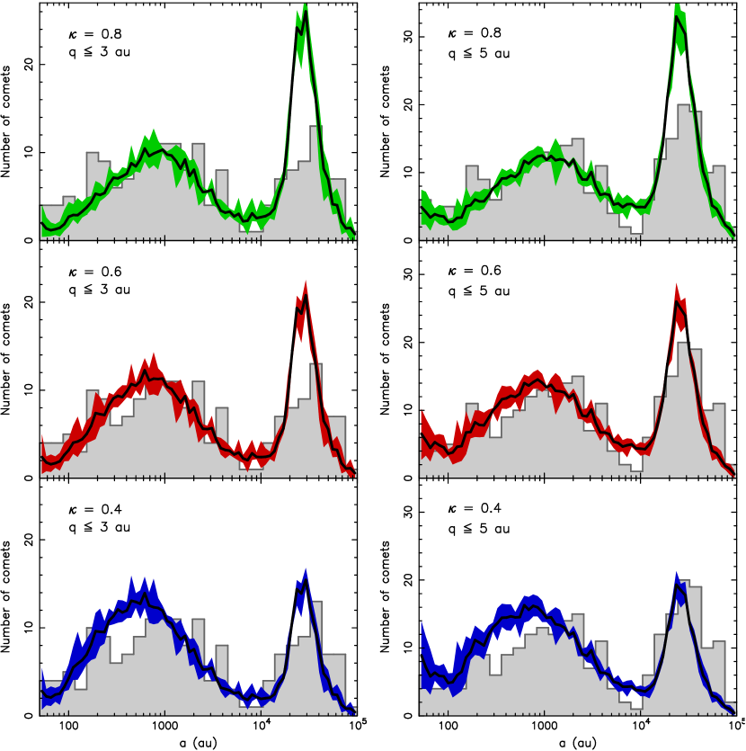
Figure 19: Comparison between data (gray histogram) and simulations for the whole population of LPCs: incremental distribution of the original semimajor axes $a$. Data use class 1 solutions in the MWC08 catalog with two constraints on perihelia: (i) left panels for $q\leq 3$ au (191 orbits), and (ii) right panels for $q\leq 5$ au (267 orbits). Simulations assume Whipple’s fading law with three different values of the power-law exponent $\kappa=0.8$ (top), $\kappa=0.6$ (middle), and $\kappa=0.4$ (bottom). Results from all four of our simulations (see Table 1) are used: the black line is their mean value and the color region is delimited by the minimum and maximum value from the runs. The simulated distributions are normalized to the total number of data points.

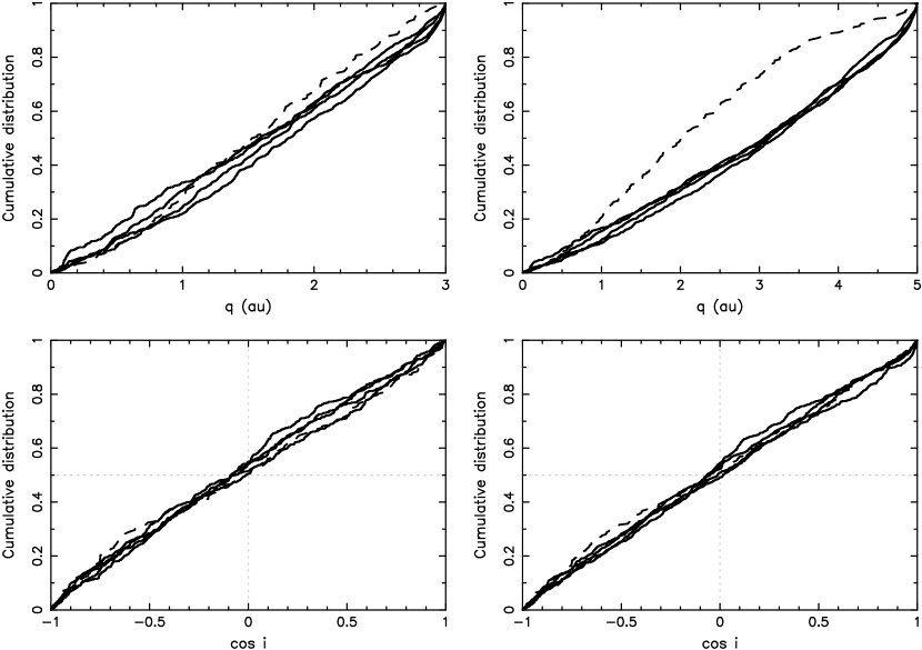
Figure 20: Comparison between data (dashed line) and simulations (solid lines) for the whole population of LPCs: cumulative distributions of perihelia (top) and cosine of ecliptic inclination (bottom). Data use class 1 solutions in the MWC08 catalog: (i) left panels for $q\leq 3$ au orbits, and (ii) right panels for $q\leq 5$ au orbits. Solid lines are results from our four simulations (see Table 1).

4.4.2 All long-period comets

As outlined in Section 2.1, the reference source for the orbits of all LPCs, including the returning ones, is the MWC08 catalog. It contains 318 accurate orbits (classes 1A and 1B), whose distribution of original semimajor axes was shown in Fig. 1. However, the distribution of their perihelia (Fig. 2) suggests the sample is still fairly incomplete beyond $q\simeq 4$ au. In order to minimize the influence of this bias, we consider sub-samples of the whole MWC08 catalog by setting a limit on the perihelion distance. For the sake of comparison, we consider two cases: (i) $q\leq 3$ au, likely less biased, but containing a smaller number of observed comets, and (ii) $q\leq 5$ au, a larger sample, but already seeing the onset of bias. As in the previous Section, we avoid the periods of the strongest comet showers in the output from our simulations in their last Gyr. To see the variance of the results of our four jobs (see Table 1), we now use all these runs. We compute the mean value of the parameter of interest and report its minimum and maximum values among the four jobs. In all cases we use Whipple’s fading law described in Section 3.6 with the only free parameter $\kappa$ being the power exponent of the life expectancy $\Phi_{n}$ through the $n$-th perihelion return. A larger value of $\kappa$ corresponds to a faster fading of new comets, while a smaller value of $\kappa$ emphasizes the role of the returning population of comets.

Figure 19 illustrates the match between the MWC08 data and our suite of simulations for comets with $q\leq 3$ au (left panels) and $q\leq 5$ au (right panels). Each time, we show results for three values of the $\kappa$ exponent: (i) $\kappa=0.8$ (top), (ii) $\kappa=0.6$ (middle), and (iii) $\kappa=0.4$ (bottom). Note that Wiegert & Tremaine (1999) obtained $\kappa=0.6\pm 0.1$ from their analysis. Clearly, the choice $\kappa=0.8$ unsuitably increases the signal in the Oort peak over the continuum of returning LPCs with semimajor axes $\leq 10000$ au for either choice of the perihelion cutoff. For the $5$ au perihelion limit, the middle value $\kappa=0.6$ appears to do the best job, and decreasing $\kappa$ to $0.4$ would already give too much weight to the population of the returning comets if compared to the Oort peak comets. Restricting the perihelion limit to $3$ au only, even $\kappa=0.4$ provides an acceptable result. So values $\kappa$ in the range $0.4$ to $0.6$ seem promising. In fact, assuming that the comet incompleteness beyond perihelia $\simeq 4$ au is dominated by the lack of observed returning comets, $\kappa=0.4$ may also satisfy the observations if some returning orbits are added.

We tried to complement such a qualitative analysis with a more rigorous, quantitative treatment of fitting the model predictions to the data. We used the MWC08 observations distributed in 27 equal-size bins in $\log a$, as shown in Fig. 19. We formally assumed $\sqrt{N}$ uncertainty statistics. We then ran the traditional least-squares fit of the fading law exponent $\kappa$ using results from our simulations. After performing this effort, we indeed obtained best values of this formal $\chi^{2}$ at $\kappa\simeq 0.6$ for $q\leq 5$ au orbits, but we noticed that the minimum normalized $\chi^{2}$ value was larger than unity (between $1.2$ and $1.4$, depending on our simulation). Restricting the orbits to $q\leq 3$ au, the formal best fit value shifted to $\kappa\simeq 0.5$, and the minimum normalized $\chi^{2}$ values were between $1.15$ and $1.25$. At face value, this should imply rejection of the model. We admit that the model is imperfect in many aspects. First, the determination of cometary orbits may have its problems, but perhaps more importantly, the fading model may be just too simple. On the other hand, we also believe that the data still suffer unrecognized systematic errors and incompleteness. As we are not able to remove these issues with the available data set, the least-squares model is plainly a formal procedure that confirms the qualitative analysis from above, but cannot improve it in a more objective way. If anything, the formal $\chi^{2}$ suggests $\kappa=0.6^{+0.1}_{-0.2}$ is the best fit to the data. This is the same result as Wiegert & Tremaine (1999) obtained, although we have a slightly larger error bar. Our allowance for slightly smaller values of $\kappa$ follows from our feeling that the population of returning comets is observationally underrepresented.

Figure 20 shows a comparison between data and simulations for the cumulative distributions of perihelion and cosine of orbital inclination with respect to the ecliptic. The left panels are for the cutoff limit $q\leq 3$ au, while the right panels are for the cutoff limit $q\leq 5$ au. In this case, we use only the simulation with $\kappa=0.6$, since inspection of other choices shows these results are not sensitive to the $\kappa$ value. The conservative restriction on perihelia, $q\leq 3$ au, leads to a fairly satisfactory match between data and model predictions. This is not surprising. Even if the suspected systematic errors bias the original values of the semimajor axes in the MWC08 catalog, the values of perihelia and inclination are much less dependent on the model uncertainty. Incompleteness may play some role beyond $q\simeq 2$ au, as may be suggested by the top left panel in Fig. 20. Obviously, things get much worse when the looser cutoff limit of $q\leq 5$ au is adopted. Here, the lack of observed comets with perihelia beyond $q\simeq 2-3$ au is obvious. In all cases, though, the isotropy of the orbital planes in space seems to match the available data.

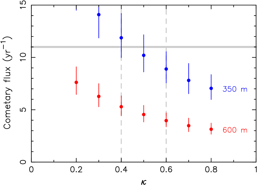
Figure 21: Predicted annual flux of LPCs with $q\leq 4$ au (ordinate) as a function of the power-law exponent $\kappa$ of Whipple’s fading law (abscissa). Results from all our four simulations (see Table 1) are used: circles give their mean value and the interval indicates minimum to maximum values in the runs. Output from the simulations was calibrated for two size values of comets: (i) $D=600$ m in red, and (ii) $D=350$ m in blue. The horizontal gray line, $11$ comets per year, is the flux for $H\leq 10.9$ LPCs reported by Francis (2005). The interval of $\kappa$ values between $0.4$ and $0.6$, vertical gray dashed lines, is our preferred range from analysis of the original semimajor axis distribution.

4.4.3 Flux of long-period comets

Finally, we confront the observed flux of LPCs with predictions from our model. We remind the reader that an obstacle to an exact comparison is that (i) the observed flux is magnitude-limited, while (ii) our model predictions are size-limited. The trouble arises because the size vs. magnitude relation for comets is uncertain.

We first focus on the model predictions. Previous applications of our framework allowed us to calibrate the trans-Neptunian planetesimal disk, namely the population of particles constituting the initial conditions of our simulations. There were about $8\times 10^{11}$ planetesimals with $D\geq 1$ km in this region, a value that may be about $50$% uncertain (Nesvorný et al., 2017). The cumulative size distribution between $1$ and nearly $100$ km may be approximated by a power law with an exponent $\simeq-2$, while the cumulative size distribution below $1$ km is uncertain, but may follow a power law with a shallower exponent $\simeq-1.5$ (see Fig. 14 in Nesvorný et al., 2017). Note that the extrapolation to sub-kilometer sizes is not as well-constrained as the size distribution for bodies with diameters $\geq 1$ km.

Next, we consider the population of simulated LPCs in the last Gyr of our runs whose orbits have a certain perihelion cutoff. In what follows, we take $q\leq 4$ au. Running analysis with different power-law exponents $\kappa$ of the Whipple fading scheme, we determine how many comets our simulations predict. We again avoid the $4$ Myr periods following the strongest stellar encounters. Having this information, we can readily predict an unbiased number of LPCs with a given size $D$ reaching, on average, their perihelia each year. Choosing two sizes $D=350$ m and $D=600$ m, we obtained the fluxes shown in Fig. 21: symbols give the mean value over our four simulations, while the associated interval indicates the minimum and maximum fluxes from these jobs. The predicted flux is correlated with $\kappa$: smaller values of this parameter lead to larger fluxes, and vice versa. This result makes sense, because a smaller $\kappa$ value lets comets live longer by surviving more perihelion returns. Our preferred values $\kappa\simeq 0.4-0.6$ imply a flux of $\simeq 3-6$ LPCs per year with $D\geq 600$ m and $q<4$ au. Note that the indicated range of the fluxes formally follows from predictions given by our four runs. In each case, we used a mean value of comet flux over a long time span of 1 Gyr. Additionally, the flux fluctuates about this mean value by up to $25$%; see the upper panels in Figs. 9, 11 and 16. Data in those figures used large bins in time, $4$ Myr, but these simulations also had a limited number of comets integrated, $10^{6}$ initially. Assuming the product of these two parameters is roughly constant, the estimated fluctuations apply to kilometer-sized comets over time period of a decade or few.

Having the fading law calibrated by the majority of observed LPCs, we also predict that the largest comet observable in two centuries should have a diameter of $\simeq(16-20)$ km. However, this is certainly an underestimate, because large comets fade much less than small comets. Consider, for instance, that HTCs, which evolve from LPCs, have been shown to typically fade only after about $3000-5000$ returns (e.g., Nesvorný et al., 2017). Therefore, the flux of large comets like Hale-Bopp (C/1995 O1) is underestimated by our analysis. For the sake of a test, we completely disregarded fading and analyzed the statistics of the observed LPCs. From this we would predict the largest LPCs seen over two centuries should have a size between $32$ and $38$ km, still somewhat smaller than the estimated sizes of the largest LPCs such as Hale-Bopp (see review in Fernández (2002); cf. Hui & Li (2018)). However, we deal with the statistics of a few objects, which may be subject to larger fluctuations.

On the side of the observed population of LPCs we recall that Francis (2005) estimated a flux of about $11$ LPCs with $q\leq 4$ au and $H\leq 10.9$ annually. Assuming the magnitude-size relation from Sosa & Fernández (2011), this magnitude limit would correspond to a size of about $600$ m. (Note, however, that the magnitude-size relations used by Francis (2005)) imply larger nuclei, with diameters $\approx 1-2$ km; see Section 2.3.) Data in Fig. 21 show that our model prediction falls short of predicting this flux by a factor of about two or three. In order to align the results with observations, the common LPCs should have a size of $\simeq 350$ m (see the blue symbols). Given the hyperactivity of LPCs, this may not be unreasonable. To check whether the flux-prediction problem could be caused by the simplicity of the fading law we used, we also computed the annual flux of new comets with $q\leq 5$ au. Assuming a typical size $D=350$ m, we obtained $4.1\pm 0.9$ (sampling again results from our four simulations). This would favorably compare with the stated $4$ new comets in this region annually (e.g. Fouchard et al., 2017a). Therefore, the fading law is likely not a problem for the flux determination. If, however, the comet flux should be higher, as indicated by the analysis of Bauer et al. (2017), or the magnitude vs. size relation should require a larger size than assumed here, the model prediction would be below the observed population of LPCs.

We thus find once again that modeling the LPC flux is the most problematic issue of their analysis. Most often researchers infer the Oort cloud population from the LPC flux. This is obviously a circular argument as far as the predictive power is concerned. Whenever previous studies attempted to use independent calibrations of the Oort cloud population, the estimates ran short of explaining the LPC flux. For instance, Brasser & Morbidelli (2013) considered model-predicted constraints on the ratio between the populations of the scattering disk and the Oort cloud. To reconcile the observed fluxes of Jupiter-family comets (JFCs) and LPCs, Brasser & Morbidelli (2013) concluded that LPCs must be systematically smaller at the same absolute magnitude than JFCs. Nonetheless, their remaining mismatch was still a bit larger than our factor of $\simeq 2-3$. Until nuclear sizes of LPCs are accurately determined from observations, most likely from future surveys of comets at large heliocentric distances, we are left with a couple of speculations.

Either LPCs are typically small, as suggested above, or the Oort cloud population is larger than we obtained. One possibility is that our assumed population of kilometer-sized planetesimals in the original trans-Neptunian disk was underestimated. In fact, their number is not constrained directly by any of the implantation processes into reservoirs of small bodies (such as Jupiter Trojans), but is set by the assumption of a shallow size distribution of the disk particles at small sizes. This is suggested by the paucity of small craters on Pluto and Charon, compared with a collisional distribution (e.g., Robbins et al., 2017; Singer et al., 2019). If those craters formed, but were then erased, however, the initial size distribution of small planetesimals might be steeper than we assumed. Another possibility is to deliver more comets into the Oort cloud than expected from our model. This could happen during the early phase when the Solar system was still in the birth cluster, or by considering a larger planetesimal source zone than we did here. Recall that our initial disk was limited to the region from Neptune’s orbit to about $30$ au. If planetesimals on initial orbits that are closer to or further from the Sun can also contribute, the Oort cloud population might be somewhat larger. Analysis of these possibilities is left for future studies.

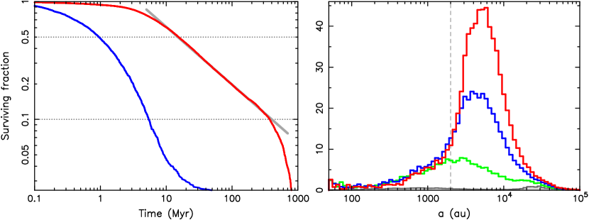
Figure 22: Left panel: Distribution of the number of comets that remained in the monitored target zone longer than time $t$. Data from the last Gyr from all our simulations combined are used, and two heliocentric radii $r$ of the target zone are plotted: (i) $r=5$ au (blue curve), and (ii) $r=20$ au (red curve). No fading is imposed, so particles are only eliminated dynamically. The gray line shows the $\propto t^{-1/2}$ power-law which matches the $r=20$ au data between $10$ and $200$ Myr well. Right panel: The same as in Fig. 13, but now with all returning particles. The distribution of original semimajor axis values for all comets in the last Gyr of our simulation C1V1 whose perihelia are in heliocentric target zones with four radii are shown: (i) $r=5$ au (gray histogram), (ii) $r=10$ au (green line), (iii) $r=15$ au (blue line), and (iv) $r=20$ au (red line). Cometary fading is applied only when the perihelion gets smaller than $5$ au (Whipple power-law scheme with $\kappa=0.6$). The ordinate is arbitrarily normalized to the maximum of the $r=5$ au plot. The total number of comets in $r\leq 20/15/10$ au zones is $\simeq 29.2/19.9/9.0$ times larger than the population entering the $r\leq 5$ au zone. The dashed vertical line points out the edge of the inner Oort cloud in our simulation.

5 Predictions for future surveys

Looking ahead to the future, perhaps the most interesting result in this paper is the prediction of a significant increase of the LPC population beyond perihelion distance $\simeq 15$ au (Fig. 12). This is not a shocking conclusion. It has already been discussed in some previous studies (e.g., Silsbee & Tremaine, 2016; Fouchard et al., 2017a), which were, however, based on simpler dynamical models. Here we present the most important features as they are predicted by our simulations. These results are mainly relevant for future well-characterized surveys such as with the Large Synoptic Survey Telescope (LSST). Unlike Silsbee & Tremaine (2016), who implemented basic features of a magnitude- and time-limited survey with a specific sky coverage, we present only the model, unbiased prediction. Constraints imposed by biases of a specific survey are not considered here.

Silsbee & Tremaine (2016) noted that LPCs with distant perihelia can roam in the trans-Saturnian region for a very long time. We find the same result. The red line in the left panel of Fig. 22 shows the distribution of time spent by comets on orbits with $q\leq 20$ au during the last Gyr of our simulations (we combined results from all runs). From about $10$ Myr, the surviving fraction of comets in this wide target zone falls-off only very slowly and is well approximated with a $t^{-1/2}$ power-law. The longest survival times, beyond about $600$ Myr, are missing in our data, but this is a result of the restricted time interval in which we monitor the cometary orbits. Very likely, the tail of the distribution will reach beyond a billion years. The exponent $-1/2$ of the time dependence is characteristic of a random walk of the orbital perihelia beyond $15$ au, at a safe distance from both Saturn and Jupiter (also see Yabushita, 1979; Silsbee & Tremaine, 2016). At the same time, the inner part of the Oort cloud can inject LPCs onto these distant-perihelion orbits with small semimajor axes, thus strongly gravitationally bound to the Solar system. Galactic tides and tugs from passing stars then feed the random walk diffusion with small steps persisting for a very long period of time. In contrast, LPCs whose perihelia reach the currently observable zone with $q\leq 5$ au, say, have the dynamical survivibility distribution shown by a blue line in the left panel of Fig. 22. These times are much shorter, a result of the typically larger semimajor axes of these comets. They are thus more weakly bound to the planetary system and are at high risk of being ejected by perturbations due to the gas giants (either direct or indirect, reflected in the motion of the Solar system barycenter).

The above-described surviving fraction distribution uses all visits of LPCs into the specified target zone within the last Gyr of our simulations. If we were to ask how much time the population of LPCs observed within the last century, say, have already spent wandering in the $q\leq 20$ au zone, the distribution would still be skewed to longer times. This is because only a fraction of short times (say $\leq 10$ Myr) would be relevant to that task as we now fix the position of the interval in time. We find that more than $50$% of LPCs with distant perihelia observed “now” have already spent more than $100$ Myr cruising the target zone, and some $15$% were injected into the planet-crossing zone more than half a billion years ago. This is in accord with conclusions in Silsbee & Tremaine (2016).

The right panel in Fig. 22 shows similar information as Fig. 13, but now extended by a population of returning comets. We use the results from the C1V1 simulation and plot a distribution of original semimajor axis values for the predicted steady-state population of LPCs reaching heliocentric zones with different perihelion cutoffs of $5/10/15/20$ au. Following methods in Silsbee & Tremaine (2016), we assume fading for comets with small perihelia only, in our case $q\leq 5$ au, certainly an approximation which needs to be refined in future comparison of the model predictions and the observations. The barely-seen gray histogram near the bottom of the plot corresponds to the currently observed population of LPCs with perihelia $q\leq 5$ au; this distribution is identical to that in the middle right panel in Fig. 19. The color-coded lines correspond to LPCs in larger perihelia zones, namely $10$ au (green), $15$ au (blue), and $20$ au (red). Increasing the cutoff limit has two main implications: (i) the number of LPCs increases rapidly beyond $15$ au (e.g., it is nearly $30$ times larger for $q\leq 20$ au, compared to the $q\leq 5$ au population); (ii) for large $q$ cutoffs the semimajor axis peaks in the inner Oort cloud zone, as this region can now efficiently feed these orbits. Our simulations show a steep drop of the distributions at about $1500$ au (blue and red lines), which reflects the edge of the created Oort cloud (see Fig. 7). However, should this edge prove to be closer – for instance, due to the existence of a fossilized inner Oort cloud extension from the birth-cluster phase of Solar system evolution – the distributions shown in the right panel of Fig. 22 would also extend to smaller $a$ values. Here again, only comparison of the model predictions with the observations will help to solve this issue.

We find that the modeled population of LPCs with perihelia $q\leq 5$ au has a slight preference for retrograde orbits (also see Fig. 20). This is in accord with predictions from other models, such as Fouchard et al. (2017a) and Silsbee & Tremaine (2016). However, the population with the largest perihelia in our model, say between $15$ au and $20$ au, shows a preference for prograde orbits (representing about $65$% of the whole sample in this category). This conclusion differs from that in Silsbee & Tremaine (2016). Recall, however, that Silsbee & Tremaine (2016) assumed an isotropic extension of the Oort cloud to its innermost part. As shown in Sec. 4.1, this assumption is not correct. The inner Oort cloud below semimajor axis $\simeq 7000$ au is strongly anisotropic, reflecting its origin in the scattering disk. Comets arriving from this part of the Oort cloud, which is the majority among the distant-perihelia orbits, remember the anisotropy of their source zone in our model.

In order to make our model useful, we prepared software which exports our results in the form of an unbiased population simulator (codes and results are available from the authors upon request). Choosing a heliocentric zone $r\leq 20$ au, it allows the user to create a catalog of LPC orbits with perihelia $q\leq r$ and whose orbits are statistically compatible with the orbital distribution from our simulations, assuming a steady-state situation. Our model also provides the LPC flux for bodies of different sizes following from the assumed initial population in the trans-Neptunian, comet-birth disk. Users can load the catalog and apply the observability efficiency of a specific survey. This way, the unbiased set of orbits from our model can generate a specific set of observable comets which can be compared with the data.

6 Conclusions

With the advent of new all-sky surveys in the forthcoming decade, we constructed a numerical model describing the origin and orbital evolution of comets. The strength of our approach consists of its being a unified scheme for all comets, both short- and long-period. The short-period comet part has been described at length in Nesvorný et al. (2017). Here we dealt with the long-period comets.

The model has several aspects. Its primary justification comes from confrontation with observations. To that end we collected all currently available data about LPCs. Surprisingly, the orbital distribution of the observed comets can still be reasonably well matched with only minimal tuning. The principal phenomenon we solved for is the LPC fading law. With the limited range of perihelion distances for which the observed sample is reasonably complete, the single-parameter model of Whipple (1962) is sufficient. The remaining differences between the data and the model predictions are small and they are plausibly explained by persisting observational biases. That said, certainly the model may also be improved in a number of aspects, but without understanding the data better, we do not see a strong need to make the model more complex. As to the LPC flux, the comparison between the observations and model is less good. While several model simplifications may be responsible for these differences, we believe that they are mainly because of the poorly-understood relationship between the size of a cometary nucleus and its absolute brightness. The model uses the sizes, while the observations provide the magnitudes. Attempts to link the two are still not completely satisfactory. Again, until these problems are resolved, far-reaching modifications of the model seem not to be justified.

Things, however, will change soon when powerful upcoming all-sky surveys will start providing observations. As far as LPCs are concerned, the crucial aspect is the extension of the perihelion range to at least $15-20$ au. Such data will offer a much more complete mapping of the Oort cloud, the source region of the long-period comets. This is because current observations effectively sample only the outermost isotropic tail of this vast source population. Its critical inner zone, still hidden to our data, contains much more information diagnostic of the history of the Solar system (both as far as its natal conditions and also the giant planets’ late migration). These future LPC observations will be able to directly probe the whole Oort cloud. Because of the likely much smaller activity of LPCs at large heliocentric distances, these new observations will also help us to clarify the current uncertainties related to their flux.

Our model allows us to provide a useful first glimpse of the expected number of comets with distant perihelia. At this moment, however, we do not feel safe to turn them into specific quantitative predictions for two reasons. First, we do not have complete information about complex observational biases, such as magnitude limits, exposure times, sky-coverage cadence, etc. In this situation, it makes more sense to provide an unbiased population prediction and work iteratively with a specific survey to fine-tune the model parameters by comparing its predictions with observations. We completed this task, but consider it a zero-order attempt. This is because an unknown aspect, likely also to be inferred from the observations, is the activity and fading of LPCs at large perihelion distances. Therefore, more advanced versions of the LPC population prediction need to be completed in the future.

References

- Adams (2010) Adams, F. C. 2010, ARA&A, 48, 47, doi: 10.1146/annurev-astro-081309-130830
- Bailer-Jones (2018) Bailer-Jones, C. A. L. 2018, A&A, 609, A8, doi: 10.1051/0004-6361/201731453
- Bailer-Jones et al. (2018) Bailer-Jones, C. A. L., Rybizki, J., Andrae, R., & Fouesneau, M. 2018, A&A, 616, A37, doi: 10.1051/0004-6361/201833456
- Bailey & Stagg (1988) Bailey, M. E., & Stagg, C. R. 1988, MNRAS, 235, 1, doi: 10.1093/mnras/235.1.1
- Bailey et al. (2016) Bailey, E., Batygin, K., & Brown, M. E. 2016, AJ, 152, 126, doi: 10.3847/0004-6256/152/5/126
- Bannister et al. (2018) Bannister, M. T., Gladman, B. J., Kavelaars, J. J., et al. 2018, ApJS, 236, 18, doi: 10.3847/1538-4365/aab77a
- Batygin et al. (2019) Batygin, K., Adams, F. C., Brown, M. E., & Becker, J. C. 2019, Phys. Rep., in the press, doi: 10.1016/j.physrep.2019.01.009
- Batygin & Brown (2016a) Batygin, K., & Brown, M. E. 2016a, AJ, 151, 22, doi: 10.3847/0004-6256/151/2/22
- Batygin & Brown (2016b) —. 2016b, ApJ, 833, L3, doi: 10.3847/2041-8205/833/1/L3
- Batygin et al. (2012) Batygin, K., Brown, M. E., & Betts, H. 2012, ApJ, 744, L3, doi: 10.1088/2041-8205/744/1/L3
- Bauer et al. (2017) Bauer, J. M., Grav, T., Fernández, Y. R., et al. 2017, AJ, 154, 53, doi: 10.3847/1538-3881/aa72df
- Berski & Dybczyński (2016) Berski, F., & Dybczyński, P. A. 2016, A&A, 595, L10, doi: 10.1051/0004-6361/201629835
- Binney & Tremaine (2008) Binney, J., & Tremaine, S. 2008, Galactic Dynamics: Second Edition (Princeton University Press)
- Bortle (1991) Bortle, J. E. 1991, International Comet Quarterly, 13, 89
- Bovy (2017) Bovy, J. 2017, MNRAS, 470, 1360, doi: 10.1093/mnras/stx1277
- Bovy & Tremaine (2012) Bovy, J., & Tremaine, S. 2012, ApJ, 756, 89, doi: 10.1088/0004-637X/756/1/89
- Brasser (2001) Brasser, R. 2001, MNRAS, 324, 1109, doi: 10.1046/j.1365-8711.2001.04400.x
- Brasser et al. (2006) Brasser, R., Duncan, M. J., & Levison, H. F. 2006, Icarus, 184, 59, doi: 10.1016/j.icarus.2006.04.010
- Brasser et al. (2007) —. 2007, Icarus, 191, 413, doi: 10.1016/j.icarus.2007.05.003
- Brasser et al. (2008) —. 2008, Icarus, 196, 274, doi: 10.1016/j.icarus.2008.02.016
- Brasser et al. (2012) Brasser, R., Duncan, M. J., Levison, H. F., Schwamb, M. E., & Brown, M. E. 2012, Icarus, 217, 1, doi: 10.1016/j.icarus.2011.10.012
- Brasser et al. (2010) Brasser, R., Higuchi, A., & Kaib, N. 2010, A&A, 516, A72, doi: 10.1051/0004-6361/201014275
- Brasser & Morbidelli (2013) Brasser, R., & Morbidelli, A. 2013, Icarus, 225, 40, doi: 10.1016/j.icarus.2013.03.012
- Brown & Batygin (2019) Brown, M. E., & Batygin, K. 2019, AJ, 157, 62, doi: 10.3847/1538-3881/aaf051
- Dones et al. (2015) Dones, L., Brasser, R., Kaib, N., & Rickman, H. 2015, Space Sci. Rev., 197, 191, doi: 10.1007/s11214-015-0223-2
- Dones et al. (2004) Dones, L., Weissman, P. R., Levison, H. F., & Duncan, M. J. 2004, Oort cloud formation and dynamics, ed. M. C. Festou, H. U. Keller, & H. A. Weaver, 153–174
- Duncan et al. (1987) Duncan, M., Quinn, T., & Tremaine, S. 1987, AJ, 94, 1330, doi: 10.1086/114571
- Dybczyński & Królikowska (2011) Dybczyński, P. A., & Królikowska, M. 2011, MNRAS, 416, 51, doi: 10.1111/j.1365-2966.2011.19005.x
- Dybczyński & Królikowska (2015) —. 2015, MNRAS, 448, 588, doi: 10.1093/mnras/stv013
- Everhart (1968) Everhart, E. 1968, AJ, 73, 1039, doi: 10.1086/110766
- Feast & Whitelock (1997) Feast, M., & Whitelock, P. 1997, MNRAS, 291, 683, doi: 10.1093/mnras/291.4.683
- Feng & Bailer-Jones (2015) Feng, F., & Bailer-Jones, C. A. L. 2015, MNRAS, 454, 3267, doi: 10.1093/mnras/stv2222
- Fernández (2005) Fernández, J. A. 2005, Comets - Nature, Dynamics, Origin and their Cosmological Relevance (Astrophysics and Space Science Library, Springer, Dordrecht)
- Fernández & Brunini (2000) Fernández, J. A., & Brunini, A. 2000, Icarus, 145, 580, doi: 10.1006/icar.2000.6348
- Fernández & Sosa (2012) Fernández, J. A., & Sosa, A. 2012, MNRAS, 423, 1674, doi: 10.1111/j.1365-2966.2012.20989.x
- Fernández (2002) Fernández, Y. R. 2002, Earth Moon and Planets, 89, 3, doi: 10.1023/A:1021545031431
- Fouchard et al. (2011a) Fouchard, M., Froeschlé, C., Rickman, H., & Valsecchi, G. B. 2011a, Icarus, 214, 334, doi: 10.1016/j.icarus.2011.04.012
- Fouchard et al. (2011b) Fouchard, M., Rickman, H., Froeschlé, C., & Valsecchi, G. B. 2011b, A&A, 535, A86, doi: 10.1051/0004-6361/201116514
- Fouchard et al. (2014) —. 2014, Icarus, 231, 110, doi: 10.1016/j.icarus.2013.11.032
- Fouchard et al. (2017a) —. 2017a, A&A, 604, A24, doi: 10.1051/0004-6361/201630343
- Fouchard et al. (2017b) —. 2017b, Icarus, 292, 218, doi: 10.1016/j.icarus.2017.01.013
- Francis (2005) Francis, P. J. 2005, ApJ, 635, 1348, doi: 10.1086/497684
- Frankel et al. (2018) Frankel, N., Rix, H.-W., Ting, Y.-S., Ness, M., & Hogg, D. W. 2018, ApJ, 865, 96, doi: 10.3847/1538-4357/aadba5
- García-Sánchez et al. (2001) García-Sánchez, J., Weissman, P. R., Preston, R. A., et al. 2001, A&A, 379, 634, doi: 10.1051/0004-6361:20011330
- Gardner et al. (2011) Gardner, E., Nurmi, P., Flynn, C., & Mikkola, S. 2011, MNRAS, 411, 947, doi: 10.1111/j.1365-2966.2010.17729.x
- Gomes et al. (2017) Gomes, R., Deienno, R., & Morbidelli, A. 2017, AJ, 153, 27, doi: 10.3847/1538-3881/153/1/27
- Gomes et al. (2015) Gomes, R. S., Soares, J. S., & Brasser, R. 2015, Icarus, 258, 37, doi: 10.1016/j.icarus.2015.06.020
- Hanse et al. (2018) Hanse, J., Jílková, L., Portegies Zwart, S. F., & Pelupessy, F. I. 2018, MNRAS, 473, 5432, doi: 10.1093/mnras/stx2721
- Heisler (1990) Heisler, J. 1990, Icarus, 88, 104, doi: 10.1016/0019-1035(90)90180-H
- Heisler & Tremaine (1986) Heisler, J., & Tremaine, S. 1986, Icarus, 65, 13, doi: 10.1016/0019-1035(86)90060-6
- Heisler et al. (1987) Heisler, J., Tremaine, S., & Alcock, C. 1987, Icarus, 70, 269, doi: 10.1016/0019-1035(87)90135-7
- Heller (1993) Heller, C. H. 1993, ApJ, 408, 337, doi: 10.1086/172591
- Higuchi & Kokubo (2015) Higuchi, A., & Kokubo, E. 2015, AJ, 150, 26, doi: 10.1088/0004-6256/150/1/26
- Higuchi et al. (2007) Higuchi, A., Kokubo, E., Kinoshita, H., & Mukai, T. 2007, AJ, 134, 1693, doi: 10.1086/521815
- Hills (1981) Hills, J. G. 1981, AJ, 86, 1730, doi: 10.1086/113058
- Hui & Li (2018) Hui, M.-T., & Li, J.-Y. 2018, PASP, 130, 104501, doi: 10.1088/1538-3873/aad538
- Kaib & Quinn (2008) Kaib, N. A., & Quinn, T. 2008, Icarus, 197, 221, doi: 10.1016/j.icarus.2008.03.020
- Kaib & Quinn (2009) —. 2009, Science, 325, 1234, doi: 10.1126/science.1172676
- Kaib et al. (2011) Kaib, N. A., Roškar, R., & Quinn, T. 2011, Icarus, 215, 491, doi: 10.1016/j.icarus.2011.07.037
- Kaib & Sheppard (2016) Kaib, N. A., & Sheppard, S. S. 2016, AJ, 152, 133, doi: 10.3847/0004-6256/152/5/133
- Królikowska (2014) Królikowska, M. 2014, A&A, 567, A126, doi: 10.1051/0004-6361/201323263
- Królikowska & Dybczyński (2010) Królikowska, M., & Dybczyński, P. A. 2010, MNRAS, 404, 1886, doi: 10.1111/j.1365-2966.2010.16403.x
- Królikowska & Dybczyński (2013) —. 2013, MNRAS, 435, 440, doi: 10.1093/mnras/stt1313
- Królikowska & Dybczyński (2017) —. 2017, MNRAS, 472, 4634, doi: 10.1093/mnras/stx2157
- Królikowska et al. (2014) Królikowska, M., Sitarski, G., Pittich, E. M., et al. 2014, A&A, 571, A63, doi: 10.1051/0004-6361/201424329
- Lai (2016) Lai, D. 2016, AJ, 152, 215, doi: 10.3847/0004-6256/152/6/215
- Levison et al. (2009) Levison, H. F., Bottke, W. F., Gounelle, M., et al. 2009, Nature, 460, 364, doi: 10.1038/nature08094
- Levison & Duncan (1994) Levison, H. F., & Duncan, M. J. 1994, Icarus, 108, 18, doi: 10.1006/icar.1994.1039
- Levison et al. (2010) Levison, H. F., Duncan, M. J., Brasser, R., & Kaufmann, D. E. 2010, Science, 329, 187, doi: 10.1126/science.1187535
- Levison et al. (2002) Levison, H. F., Morbidelli, A., Dones, L., et al. 2002, Science, 296, 2212, doi: 10.1126/science.1070226
- Marsden & Sekanina (1973) Marsden, B. G., & Sekanina, Z. 1973, AJ, 78, 1118, doi: 10.1086/111516
- Marsden et al. (1978) Marsden, B. G., Sekanina, Z., & Everhart, E. 1978, AJ, 83, 64, doi: 10.1086/112177
- Marsden et al. (1973) Marsden, B. G., Sekanina, Z., & Yeomans, D. K. 1973, AJ, 78, 211, doi: 10.1086/111402
- Marsden & Williams (2008) Marsden, B. G., & Williams, G. V. 2008, Catalogue of Cometary Orbits 2008, 17th Edition (IAU Minor Planet Center/Central Bureau for Astronomical Telegrams, Cambridge, MA)
- Martínez-Barbosa et al. (2015) Martínez-Barbosa, C. A., Brown, A. G. A., & Portegies Zwart, S. 2015, MNRAS, 446, 823, doi: 10.1093/mnras/stu2094
- Martínez-Barbosa et al. (2017) Martínez-Barbosa, C. A., Jílková, L., Portegies Zwart, S., & Brown, A. G. A. 2017, MNRAS, 464, 2290, doi: 10.1093/mnras/stw2507
- Nesvorný (2015a) Nesvorný, D. 2015a, AJ, 150, 73, doi: 10.1088/0004-6256/150/3/73
- Nesvorný (2015b) —. 2015b, AJ, 150, 68, doi: 10.1088/0004-6256/150/3/68
- Nesvorný & Morbidelli (2012) Nesvorný, D., & Morbidelli, A. 2012, AJ, 144, 117, doi: 10.1088/0004-6256/144/4/117
- Nesvorný & Vokrouhlický (2016) Nesvorný, D., & Vokrouhlický, D. 2016, ApJ, 825, 94, doi: 10.3847/0004-637X/825/2/94
- Nesvorný et al. (2014) Nesvorný, D., Vokrouhlický, D., & Deienno, R. 2014, ApJ, 784, 22, doi: 10.1088/0004-637X/784/1/22
- Nesvorný et al. (2017) Nesvorný, D., Vokrouhlický, D., Dones, L., et al. 2017, ApJ, 845, 27, doi: 10.3847/1538-4357/aa7cf6
- Nesvorný et al. (2013) Nesvorný, D., Vokrouhlický, D., & Morbidelli, A. 2013, ApJ, 768, 45, doi: 10.1088/0004-637X/768/1/45
- Nesvorný et al. (2016) Nesvorný, D., Vokrouhlický, D., & Roig, F. 2016, ApJ, 827, L35, doi: 10.3847/2041-8205/827/2/L35
- Nordlander et al. (2017) Nordlander, T., Rickman, H., & Gustafsson, B. 2017, A&A, 603, A112, doi: 10.1051/0004-6361/201630342
- Oort (1950) Oort, J. H. 1950, Bull. Astron. Inst. Netherlands, 11, 91
- Pfalzner et al. (2015) Pfalzner, S., Davies, M. B., Gounelle, M., et al. 2015, Phys. Scr, 90, 068001, doi: 10.1088/0031-8949/90/6/068001
- Rickman (2010) Rickman, H. 2010, in Lecture Notes in Physics, Berlin Springer Verlag, Vol. 790, Lecture Notes in Physics, Berlin Springer Verlag, ed. J. Souchay & R. Dvorak, 341–399
- Rickman et al. (2008) Rickman, H., Fouchard, M., Froeschlé, C., & Valsecchi, G. B. 2008, Celestial Mechanics and Dynamical Astronomy, 102, 111, doi: 10.1007/s10569-008-9140-y
- Robbins et al. (2017) Robbins, S. J., Singer, K. N., Bray, V. J., et al. 2017, Icarus, 287, 187, doi: 10.1016/j.icarus.2016.09.027
- Roškar et al. (2008) Roškar, R., Debattista, V. P., Quinn, T. R., Stinson, G. S., & Wadsley, J. 2008, ApJ, 684, L79, doi: 10.1086/592231
- Rozehnal et al. (2016) Rozehnal, J., Brož, M., Nesvorný, D., et al. 2016, MNRAS, 462, 2319, doi: 10.1093/mnras/stw1719
- Sekanina (2019) Sekanina, Z. 2019, arXiv:1903.06300
- Shankman et al. (2017) Shankman, C., Kavelaars, J. J., Bannister, M. T., et al. 2017, AJ, 154, 50, doi: 10.3847/1538-3881/aa7aed
- Silsbee & Tremaine (2016) Silsbee, K., & Tremaine, S. 2016, AJ, 152, 103, doi: 10.3847/0004-6256/152/4/103
- Singer et al. (2019) Singer, K. N., McKinnon, W. B., Gladman, B., et al. 2019, Science, 363, 955
- Sosa & Fernández (2011) Sosa, A., & Fernández, J. A. 2011, MNRAS, 416, 767, doi: 10.1111/j.1365-2966.2011.19111.x
- Thies et al. (2005) Thies, I., Kroupa, P., & Theis, C. 2005, MNRAS, 364, 961, doi: 10.1111/j.1365-2966.2005.09644.x
- Trujillo & Sheppard (2014) Trujillo, C. A., & Sheppard, S. S. 2014, Nature, 507, 471, doi: 10.1038/nature13156
- Tsiganis et al. (2005) Tsiganis, K., Gomes, R., Morbidelli, A., & Levison, H. F. 2005, Nature, 435, 459, doi: 10.1038/nature03539
- Vokrouhlický et al. (2016) Vokrouhlický, D., Bottke, W. F., & Nesvorný, D. 2016, AJ, 152, 39, doi: 10.3847/0004-6256/152/2/39
- Vokrouhlický & Nesvorný (2015) Vokrouhlický, D., & Nesvorný, D. 2015, ApJ, 806, 143, doi: 10.1088/0004-637X/806/1/143
- Weber & de Boer (2010) Weber, M., & de Boer, W. 2010, A&A, 509, A25, doi: 10.1051/0004-6361/200913381
- Weissman (1990) Weissman, P. R. 1990, in Global Catastrophes in Earth History; An Interdisciplinary Conference on Impacts, Volcanism, and Mass Mortality, Vol. 247, Geological Society of America, 171–180
- Whipple (1962) Whipple, F. L. 1962, AJ, 67, 1, doi: 10.1086/108596
- Whipple (1978) —. 1978, Moon and Planets, 18, 343, doi: 10.1007/BF00896489
- Whipple (1992) —. 1992, Celestial Mechanics and Dynamical Astronomy, 54, 1, doi: 10.1007/BF00049540
- Wiegert & Tremaine (1999) Wiegert, P., & Tremaine, S. 1999, Icarus, 137, 84, doi: 10.1006/icar.1998.6040
- Wong & Brown (2015) Wong, I., & Brown, M. E. 2015, AJ, 150, 174, doi: 10.1088/0004-6256/150/6/174
- Yabushita (1979) Yabushita, S. 1979, MNRAS, 187, 445, doi: 10.1093/mnras/187.3.445
- Yoshida & Terai (2017) Yoshida, F., & Terai, T. 2017, AJ, 154, 71, doi: 10.3847/1538-3881/aa7d03