Transfer Learning for Clinical Time Series Analysis using Deep Neural Networks

Abstract

Deep neural networks have shown promising results for various clinical prediction tasks such as diagnosis, mortality prediction, predicting duration of stay in hospital, etc. However, training deep networks – such as those based on Recurrent Neural Networks (RNNs) – requires large labeled data, significant hyper-parameter tuning effort and expertise, and high computational resources. In this work, we investigate as to what extent can transfer learning address these issues when using deep RNNs to model multivariate clinical time series. We consider two scenarios for transfer learning using RNNs: i) domain-adaptation, i.e., leveraging a deep RNN – namely, TimeNet – pre-trained for feature extraction on time series from diverse domains, and adapting it for feature extraction and subsequent target tasks in healthcare domain, ii) task-adaptation, i.e., pre-training a deep RNN – namely, HealthNet – on diverse tasks in healthcare domain, and adapting it to new target tasks in the same domain. We evaluate the above approaches on publicly available MIMIC-III benchmark dataset, and demonstrate that (a) computationally-efficient linear models trained using features extracted via pre-trained RNNs outperform or, in the worst case, perform as well as deep RNNs and statistical hand-crafted features based models trained specifically for target task; (b) models obtained by adapting pre-trained models for target tasks are significantly more robust to the size of labeled data compared to task-specific RNNs, while also being computationally efficient. We, therefore, conclude that pre-trained deep models like TimeNet and HealthNet allow leveraging the advantages of deep learning for clinical time series analysis tasks, while also minimize dependence on hand-crafted features, deal robustly with scarce labeled training data scenarios without overfitting, as well as reduce dependence on expertise and resources required to train deep networks from scratch (e.g. neural network architecture selection and hyper-parameter tuning efforts).

1 Introduction

Electronic health records (EHR) consisting of a patient’s medical history can be leveraged for various clinical applications such as diagnosis, recommending medicine, etc. Traditional machine learning techniques often require careful domain-specific feature engineering before building the prediction models. On the other hand, deep learning approaches enable end-to-end learning without the need of hand-crafted and domain-specific features, and have recently produced promising results for various clinical prediction tasks (Lipton et al., 2015; Miotto et al., 2017; Ravì et al., 2017). Given this, there has been a rapid growth in the applications of deep learning to various clinical prediction tasks from Electronic Health Records, e.g. Doctor AI (Choi et al., 2016) for medical diagnosis, Deep Patient (Miotto et al., 2016) to predict future diseases in patients, DeepR (Nguyen et al., 2017) to predict unplanned readmission after discharge, etc. With various medical parameters being recorded over a period of time in EHR databases, Recurrent Neural Networks (RNNs) can be an effective way to model the sequential aspects of EHR data, e.g. diagnoses (Lipton et al., 2015; Che et al., 2016; Choi et al., 2016), mortality prediction and estimating length of stay (Harutyunyan et al., 2017; Purushotham et al., 2017; Rajkomar et al., 2018).

However, RNNs require large labeled data for training like any other deep learning approach and are prone to overfitting when labeled training data is scarce, and often require careful and computationally-expensive hyper-parameter tuning effort. Transfer learning (Pan and Yang, 2010; Bengio, 2012) has been demonstrated to be useful to address some of these challenges. It enables knowledge transfer from neural networks trained on a source task (domain) with sufficient training instances to a related target task (domain) with few training instances. For example, training a deep network on diverse set of images can provide useful features for images from unseen domains (Simonyan and Zisserman, 2014). Moreover, fine-tuning a pre-trained network for target task is often faster and easier than constructing and training a new network from scratch (Bengio, 2012; Malhotra et al., 2017).

It has been shown that pre-trained networks can learn to extract a rich set of generic features that can then be applied to a wide range of other similar tasks (Malhotra et al., 2017). Also, it has been argued that transferring weights even from distant tasks can be better than using random initial weights (Yosinski et al., 2014). Transfer learning via fine-tuning parameters of pre-trained models for end tasks has been recently considered for medical applications as well, e.g. (Choi et al., 2016; Lee et al., 2017). However, fine-tuning a large number of parameters with a small labeled dataset may still result in overfitting, and requires careful regularization (as we show in Section 9 through empirical evaluation).

In this work, we propose two simple yet effective approaches to transfer the knowledge captured in pre-trained deep RNNs for new target tasks in healthcare domain. More specifically, we consider two scenarios: i) extract features from a pre-trained network and use them to build models for target task, ii) initialize deep network for target task using parameters of a pre-trained network and then fine-tune using labeled training data for target task. The key contributions of this work are:

• We propose two approaches for transfer learning using deep RNNs for classification tasks such as patient phenotyping and mortality prediction given the multivariate time series corresponding to physiological parameters of patients. We show effective approaches to adapt: i) general-purpose time series feature extractor based on deep RNNs (TimeNet, Malhotra et al. (2017), detailed in Section 5) while overcoming the need to train a deep neural network from scratch while still leveraging its advantages, ii) a deep RNN trained specifically for healthcare domain (HealthNet, detailed in Section 6) while requiring significantly lesser amount of labeled training data for target task and significantly small hyper-parameter tuning effort.

• Our proposed approaches allow to extract robust features from variable length multivariate time series by using pre-trained deep RNNs, thereby reducing dependence on expert domain-driven feature extraction. We demonstrate that simple linear classification models trained on time series features extracted from our pre-trained models yield significantly better results compared to models trained using carefully extracted statistical features or deep RNN models trained from scratch specifically for the target task.

• We show that carefully regularized fine-tuning of pre-trained RNNs leads to models that are significantly more robust to training data sizes, and yield models that are significantly better compared to task-specific deep as well as shallow classification models trained from scratch, especially when training data is small.

Through empirical evaluation on patient phenotyping and mortality predictions tasks on MIMIC-III benchmark dataset (Johnson et al., 2016) (as described in Section 8 and 9), we demonstrate that our transfer learning approaches yield data- and compute-efficient classification models that require little training effort while yielding performance comparable to models with hand-crafted features or carefully trained domain-specific deep networks benchmarked in (Harutyunyan et al., 2017; Song et al., 2017).

The rest of the paper is organized as follows: In Section 2 we present some related work, and describe details of TimeNet in Section 3. We provide an overview of the proposed approaches in Section 4, and provide their details in Section 5 and Section 6. We provide cohort selection and other details of dataset considered in Section 7. We provide experimental details and observations made in Section 8 and Section 9 respectively, and finally conclude in Section 10.

2 Related Work

Transfer Learning via Feature Extraction TimeNet-based features have been shown to be useful for various tasks including ECG classification (Malhotra et al., 2017). In this work, we consider application of TimeNet to phenotyping and in-hospital mortality tasks for multivariate clinical time series classification. Deep Patient (Miotto et al., 2016) proposes leveraging features from a pre-trained stacked-autoencoder for EHR data. However, it does not leverage the temporal aspect of the data and uses a non-temporal model based on stacked-autoencoders. Our approach extracts temporal features via TimeNet incorporating the sequential nature of EHR data. Doctor AI (Choi et al., 2016) uses discretized medical codes (e.g. diagnosis, medication, procedure) from longitudinal patient visits via a purely supervised setting while we use real-valued time series. While approaches like Doctor AI require training a deep RNN from scratch, our approach leverages a general-purpose RNN for feature extraction.

(Harutyunyan et al., 2017) consider training a deep RNN model for multiple prediction tasks simultaneously including phenotyping and in-hospital mortality to learn a general-purpose deep RNN for clinical time series. They show that it is possible to train a single network for multiple tasks simultaneously by capturing generic features that work across different tasks. We also consider leveraging generic features for clinical time series but using an RNN that is pre-trained on diverse time series across domains, making our approach more efficient. Further, we provide an approach to rank the raw input features in order of their relevance that helps validate the models learned.

Transfer Learning via Fine-tuning Unsupervised pre-training has been shown to be effective in capturing the generic patterns and distribution from EHR data (Miotto et al., 2016). Further, RNNs for time series classification from EHR data have been successfully explored, e.g. in (Lipton et al., 2015; Che et al., 2016). However, these approaches do not address the challenge posed by limited labeled data, which is the focus of this work. Transfer learning using deep neural networks has been recently explored for medical applications: A model learned from one hospital could be adapted to another hospital for same task via recurrent neural networks (Choi et al., 2016). A deep neural network was used to transfer knowledge from one dataset to another while the source and target tasks (named-entity recognition from medical records) are the same in (Lee et al., 2017). However, in both these transfer learning approaches, the source and target tasks are the same while only the dataset changes.

In this work, we provide an approach to transfer the model trained on several healthcare-specific tasks to a different (although related) classification task using RNNs for clinical time series. Training a deep RNN for multiple related tasks simultaneously on clinical time series has been shown to improve the performance for all tasks (Harutyunyan et al., 2017). In this work, we additionally demonstrate that a model trained in this manner serves as a good initializer for building models for new related tasks.

3 Background: TimeNet

Deep (multi-layered) RNNs have been shown to perform hierarchical processing of time series with different layers tackling different time scales (Hermans and Schrauwen, 2013; Malhotra et al., 2015). TimeNet (Malhotra et al., 2017) is a general-purpose multi-layered RNN trained on large number of diverse univariate time series from UCR Time Series Archive (Chen et al., 2015) that has been shown to be useful as off-the-shelf feature extractor for time series. TimeNet has been trained on 18 different datasets simultaneously via an RNN autoencoder in an unsupervised manner for reconstruction task. Features extracted from TimeNet have been found to be useful for classification task on 30 datasets not seen during training of TimeNet, proving its ability to provide meaningful features for unseen datasets.

(a)

(b)

Figure 1: (a) TimeNet trained via RNN Encoder-Decoder with three hidden GRU layers, (b) TimeNet based Feature Extraction. TimeNet is shown unrolled for L = 3.

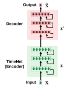
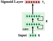
TimeNet contains three recurrent layers having 60 Gated Recurrent Units (GRUs) (Cho et al., 2014) each. TimeNet is an RNN trained via an autoencoder consisting of an encoder RNN and a decoder RNN trained simultaneously using the sequence-to-sequence learning framework (Sutskever et al., 2014; Bahdanau et al., 2014) as shown in Figure 1. RNN autoencoder is trained to obtain the parameters $\mathbf{W}_{E}$ of the encoder RNN $f_{E}$ via reconstruction task such that for input $x_{1\ldots\tau}=x_{1},x_{2},...,x_{\tau}$ ($x_{i}\in\mathbb{R}$), the target output time series $x_{\tau\ldots 1}=x_{\tau},x_{\tau-1},...,x_{1}$ is reverse of the input.

The RNN encoder $f_{E}$ provides a non-linear mapping of the univariate input time series to a fixed-dimensional vector representation $\mathbf{z}_{\tau}$ : $\mathbf{z}_{\tau}=f_{E}(x_{1\ldots\tau};\mathbf{W}_{E})$, followed by an RNN decoder $f_{D}$ based non-linear mapping of $\mathbf{z}_{\tau}$ to univariate time series: $\hat{x}_{\tau\ldots 1}=f_{D}(\mathbf{z}_{\tau};\mathbf{W}_{D})$; where $\mathbf{W}_{E}$ and $\mathbf{W}_{D}$ are the parameters of the encoder and decoder, respectively. The model is trained to minimize the average squared reconstruction error. Training on 18 diverse datasets simultaneously results in robust time series features getting captured in $\mathbf{z}_{\tau}$: the decoder relies on $\mathbf{z}_{\tau}$ as the only input to reconstruct the time series, forcing the encoder to capture all the relevant information in the time series into the fixed-dimensional vector $\mathbf{z}_{\tau}$. This vector $\mathbf{z}_{\tau}$ is used as the feature vector for input $x_{1\ldots\tau}$. This feature vector is then used to train a simpler classifier (e.g. SVM, as used in (Malhotra et al., 2017)) for the end task. TimeNet maps a univariate input time series to 180-dimensional feature vector, where each dimension corresponds to final output of one of the 60 GRUs in the 3 recurrent layers.

4 Approach Overview

Consider sets $\mathcal{D}_{S}$ and $\mathcal{D}_{T}$ of time series instances corresponding to source ($S$) and target ($T$) dataset, respectively. $\mathcal{D}_{S}=\{(\mathbf{x}_{S}^{(i)},\mathbf{y}_{S}^{(i)})\}_{i=1}^{N_{S}}$, where $N_{S}$ is the number of time series instances in the source dataset. Denoting time series $\mathbf{x}^{(i)}_{S}$ by $\mathbf{x}$ and the corresponding target label $\mathbf{y}_{S}^{(i)}$ by $\mathbf{y}$ for simplicity of notation, we have $\mathbf{x}=\mathbf{x}_{1}\mathbf{x}_{2}\ldots\mathbf{x}_{\tau}$ denote a time series of length $\tau$, where $\mathbf{x}_{t}\in\mathbb{R}^{n}$ is an $n$-dimensional vector corresponding to $n$ parameters. Further, $\mathbf{y}=[y_{1},\ldots,y_{K}]\in\{0,1\}^{K}$, where $K$ is the number of binary classification tasks. Similarly, $\mathcal{D}_{T}=\{(\mathbf{x}_{T}^{(i)},y_{T}^{(i)})\}_{i=1}^{N_{T}}$ such that $N_{T}\ll N_{S}$ , and $y_{T}^{(i)}\in\{0,1\}$ such that the target task is a binary classification task. We consider $\mathcal{D}_{S}$ and $\mathcal{D}_{T}$ to be from same (different) domain if the $n$ parameters in $\mathcal{D}_{S}$ and $\mathcal{D}_{T}$ are the same (different). Further, we consider the $tasks$ for $\mathcal{D}_{S}$ and $\mathcal{D}_{T}$ to be the same if number of target classes in $\mathbf{y}_{T}$ and $\mathbf{y}_{S}$ are equal and corresponding classes are semantically same e.g. both $\mathbf{y}_{S}$ and $\mathbf{y}_{T}$ corresponding to two classes {patient survives, patient dies}.

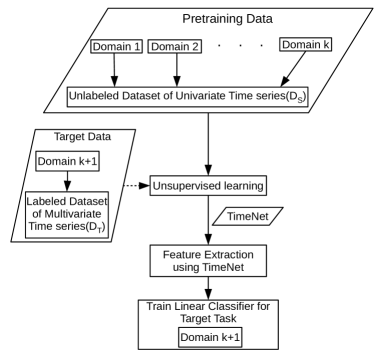
We consider two scenarios for transfer learning using RNNs: i) domain adaptation, $\mathcal{D}_{S}$ contains time series from various domains such as electric devices, motion capture, spectrographs, sensor readings, ECGs, simulated time series, etc taken from publicly available UCR Time Series Classification Archive (Chen et al., 2015), and $\mathcal{D}_{T}$ contains clinical time series from EHR database (set $\mathcal{D}_{T}$ and $\mathcal{D}_{S}$ are from different domain). We consider pre-training RNN model using $\mathcal{D}_{S}$ via unsupervised learning, which can provide useful features for time series from unseen domain (healthcare in our case). We adapt pre-trained model using $\mathcal{D}_{T}$ via supervised learning (Note: As we adapt model trained via unsupervised learning for supervised task, set $\mathcal{D}_{T}$ and $\mathcal{D}_{S}$ are from different task). ii) task adaptation, $\mathcal{D}_{S}$ and $\mathcal{D}_{T}$ contain time series from same domain i.e. healthcare, $\mathbf{x}_{S}$ and $\mathbf{x}_{T}$ corresponding to same $n$ physiological parameters e.g. heart rate, pulse rate, oxygen saturation, etc. Further, $\mathbf{y}_{S}$ corresponds to various tasks, such as presence/absence of phenotypes e.g. acute cerebrovascular disease, diabetes mellitus with complications, gastrointestinal hemorrhage, etc., and $\mathbf{y}_{T}$ corresponds to a related but different task e.g. present/absence of new phenotypes that are not present in $\mathbf{y}_{S}$ and mortality prediction. We consider pre-training an RNN model using $\mathcal{D}_{S}$ via supervised learning on a diverse set of tasks such that the model learns to capture and extract a rich set of generic features from time series that can be useful for other tasks in same domain. We adapt pre-trained model using $\mathcal{D}_{T}$ via supervised learning.

5 Domain-adaptation: adapting universal time series feature extractors to healthcare domain

Figure 2: Domain-adaptation Scenario. A deep RNN (TimeNet) is pre-trained in an unsupervised manner on time series from $k$ diverse domains, and then used for time series feature extraction from $(k+1)$-th domain and subsequent classification.

General-purpose time series feature extractors such as TimeNet and Universal Encoder (Serra et al., 2018) usually constrain the input time series to be univariate as it is difficult to cater to multivariate time series with varying dimensionality in a single neural network. In this scenario, we consider adapting TimeNet to healthcare domain with two key considerations: 1) use TimeNet that caters to univariate time series for multivariate clinical time series which requires simultaneous consideration of various physiological parameters, 2) adapt the features from TimeNet for specific tasks from healthcare such as patient phenotyping and mortality prediction tasks. We show how TimeNet can be adapted to these classification tasks by training computationally efficient traditional linear classifiers on top of features extracted from TimeNet as shown in Figure 2. Further, we propose a simple mechanism to leverage the weights of the trained linear classifier to provide insights into the relevance of each raw input feature (physiological parameter) for a given phenotype (described in Section 5.3).

Consider $\mathcal{D}_{T}$ is set of labeled time series instances from an EHR database: $\mathcal{D}_{T}=\{(\mathbf{x}_{T}^{(i)},y_{T}^{(i)})\}_{i=1}^{N_{T}}$, where $\mathbf{x}_{T}^{(i)}$ is a multivariate time series, $y_{T}^{(i)}\in\{0,1\}$ such that the target task is a binary classification task, $N_{T}$ is the number of time series instances corresponding to patients. We consider presence or absence of a phenotype as a binary classification task, and learn an independent model for each phenotype (unlike Harutyunyan et al. (2017) which consider phenotyping as a multi-label classification problem). This allows us to build simple and compute-efficient linear binary classification models as described next in Section 5.2. In practice, the outputs of these binary classifiers can then be considered together to estimate the set of phenotypes present in a patient. Similarly, mortality prediction is considered to be a binary classification task where the goal is to classify whether the patient will survive (after admission to ICU) or not.

5.1 Feature Extraction for Multivariate Clinical Time Series

Figure 3: TimeNet based Feature Extraction and Classification.

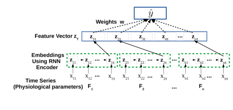
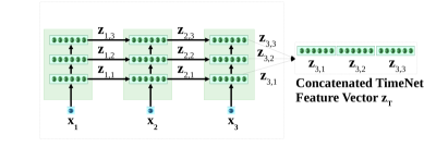
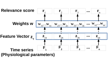
For a multivariate time series $\mathbf{x}=\mathbf{x}_{1}\mathbf{x}_{2}\ldots\mathbf{x}_{\tau}$, where $\mathbf{x}_{t}\in\mathbb{R}^{n}$, we consider time series for each of the $n$ raw input features (physiological parameters, e.g. glucose level, heart rate, etc.) independently, to obtain univariate time series $x_{j}={x}_{j1}{x}_{j2}\ldots{x}_{j\tau}$, $j~{}=1\ldots n$. (Note: We use $\mathbf{x}$ instead of $\mathbf{x}^{(i)}$ and omit superscript $(i)$ for ease of notation). We obtain the vector representation $\mathbf{z}_{j\tau}=f_{E}(x_{j};\mathbf{W}_{E}$) for $x_{j}$, where $\mathbf{z}_{j\tau}\in\mathbb{R}^{c}$ using TimeNet as $f_{E}$ with $c=180$ (as described in Section 3). In general, time series length $\tau$ also depends on $i$, e.g. based on length of stay in hospital. We omit this for sake of clarity without loss of generality. In practice, we convert each time series to have equal length $\tau$ by suitable pre/post-padding with 0s. We concatenate the TimeNet-features $\mathbf{z}_{j\tau}$ for each raw input feature $j$ to get the final feature vector $\mathbf{z}_{\tau}=[\mathbf{z}_{1\tau},\mathbf{z}_{2\tau},\ldots,\mathbf{z}_{n\tau}]$ for time series $\mathbf{x}$, where $\mathbf{z}_{\tau}\in\mathbb{R}^{m}$, $m=n\times c$ as illustrated in Figure 3.

5.2 Using TimeNet-based Features for Classification

The final concatenated feature vector $\mathbf{z}_{\tau}$ is used as input for the phenotyping and mortality prediction classification tasks. We note that since $c=180$ is large, $\mathbf{z}_{\tau}$ has large number of features $m\geq 180$. We consider a linear mapping from input TimeNet features $\mathbf{z}_{\tau}$ to the target label $y$ s.t. the estimate $\hat{y}=\mathbf{w}\cdot\mathbf{z}_{\tau}$, where $\mathbf{w}\in\mathbb{R}^{m}$. We constrain the linear model with weights $\mathbf{w}$ to use only a few of these large number of features. The weights are obtained using LASSO-regularized loss function Tibshirani (1996):

$$\operatorname*{arg\,min}_{\mathbf{w}}\frac{1}{N}\sum_{i=1}^{N}(y^{(i)}-\mathbf{w}\cdot\mathbf{z}_{\tau}^{(i)})^{2}+\alpha||\mathbf{w}||_{1}$$ (1)

where $y^{(i)}\in\{0,1\}$, $||\mathbf{w}||_{1}=\sum_{j=1}^{n}\sum_{k=1}^{c}|w_{jk}|$ is the L₁-norm, where $w_{jk}$ represents the weight assigned to the $k$-th TimeNet-feature for the $j$-th raw feature, and $\alpha$ controls the extent of sparsity – with higher $\alpha$ implying more sparsity, i.e. fewer TimeNet features are selected for the final classifier.

Figure 4: Obtaining relevance scores for raw input features. Here, $\tau$: time series length, $n$: number of raw input features.

5.3 Obtaining Relevance Scores for Raw Features

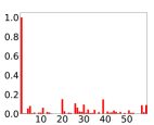
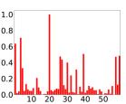
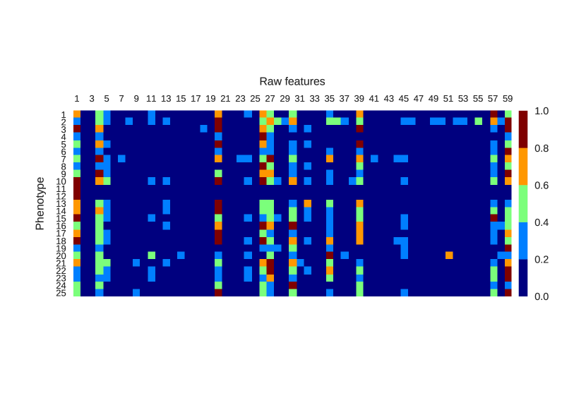
Determining relevance of the $n$ raw input features for a given phenotype is potentially useful to obtain insights into the obtained classification model. The sparse weights $\mathbf{w}$ are easy to interpret and can give interesting insights into relevant features for a classification task (e.g. as used in Micenková et al. (2013)). We obtain the relevance $r_{j}$ of the $j$-th raw input feature as the sum of the absolute values of the weights $w_{jk}$ assigned to the corresponding TimeNet features $\mathbf{z}_{j\tau}$ as shown in Figure 4, s.t.

$$r_{j}=\sum_{k=1}^{c}|w_{jk}|,~{}j=1\ldots n.$$ (2)

Further, $r_{j}$ is normalized using min-max normalization such that $r^{\prime}_{j}=\frac{r_{j}-r_{min}}{r_{max}-r_{min}}\in[0,1]$; $r_{min}$ is minimum of $\{r_{1},\ldots,r_{n}\}$, $r_{max}$ is maximum of $\{r_{1},\ldots,r_{n}\}$. In practice, this kind of relevance scores for the raw features help to interpret and validate the overall model. For example, one would expect blood glucose level feature to have a high relevance score when learning a model to detect diabetes mellitus phenotype (we provide such insights later in Section 8).

6 Task-adaptation: adapting healthcare-specific pre-trained models to a new task

Figure 5: Task-adaptation Scenario. A deep RNN (HealthNet) is pre-trained for $K$ classification tasks from healthcare domain simultaneously via supervised training. Then, it is adapted for target task either via fine-tuning or feature extraction (potentially using only a small amount of labeled training data for target task).

(a)

(b)

Figure 6: (a) HealthNet trained via supervised learning for multiple source tasks simultaneously using final activation as sigmoid, (b) fine-tuning HealthNet for a new target task using final activation as softmax. Here, blue and red arrows corresponds to recurrent and feed forward weights of the recurrent layers respectively. Only feed forward (red) weights are regularized while fine-tuning the HealthNet. RNN with L = 2 hidden layers is shown unrolled over $\tau$ = 3 time steps.

Figure 7: Inference in Task-Adaptation: Using features extracted from HealthNet. RNN with $L=2$ hidden layers is shown unrolled over $\tau=3$ time steps.

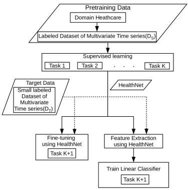
In this scenario, the goal is to transfer the learning from a set of tasks to another related task for clinical time series by means of an RNN. Considering phenotype detection from time series of physiological parameters as a binary classification task, we train HealthNet as an RNN classifier on a diverse set of such binary classification tasks (one task per phenotype) simultaneously using a large labeled dataset. We consider following approaches to adapt it to an unseen target task as shown in Figure 5:

1. We initialize parameters of the target task specific RNN using the parameters of HealthNet previously trained on a large number of source tasks; so that HealthNet provides good initialization of parameters of task-specific RNN and train the model (described in Section 6.2).

2. We extract features using HealthNet and then train an easily trainable non-temporal linear classification model such as a logistic regression model (Hosmer Jr et al., 2013) for target tasks, i.e. identifying a new phenotype and predicting in-hospital mortality, with few labeled instances (described in Section 6.3).

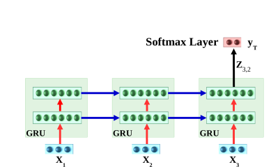
More specifically, consider $\mathcal{D}S$ and $\mathcal{D}_{T}$ are sets of labeled time series instances from an EHR database (i.e. same $domain$): $\mathcal{D}_{S}=\{(\mathbf{x}_{S}^{(i)},\mathbf{y}_{S}^{(i)})\}_{i=1}^{N_{S}}$, where $\mathbf{x}_{S}^{(i)}$ is a multivariate time series, $\mathbf{y}_{S}^{(i)}=\{y_{1},\ldots,y_{K}\}\in\{0,1\}^{K}$, $K$ is the number of binary classification tasks, $N_{S}$ is the number of time series instances corresponding to patients. Similarly, $\mathcal{D}_{T}=\{(\mathbf{x}_{T}^{(i)},y_{T}^{(i)})\}_{i=1}^{N_{T}}$ such that $N_{T}\ll N_{S}$, and $y_{T}^{(i)}\in\{0,1\}$ such that the target task is a binary classification task. We first train HealthNet on $K$ source tasks using $\mathcal{D}_{S}$ (refer Section 6.1 for details), as shown in Figure 6(a), and then consider following two scenarios for adapting to the target tasks using $\mathcal{D}_{T}$:

• fine-tuning the HealthNet with suitable regularization (refer Section 6.2 for details), as shown in Figure 6(b). This allow us to train model that does not require hyper-parameter tuning efforts.

• train the simpler logistic regression (LR) classifier for target task using $\mathcal{D}_{T}$ and the features obtained via HealthNet (refer Section 6.3 for details), as shown in Figure 7, which is compute-efficient.

We next provide details of training RNN and LR models.

6.1 Obtaining HealthNet using Supervised Pre-training of RNN

Training an RNN on $K$ binary classification tasks simultaneously can be considered as a multi-label classification problem. We train a multi-layered RNN with $L$ recurrent layers having Gated Recurrent Units (GRUs) (Cho et al., 2014) to map $\mathbf{x}^{(i)}\in\mathcal{D}_{S}$ to $\mathbf{y}^{(i)}$. Let $\mathbf{z}_{t,l}\in\mathbb{R}^{h}$ denote the output of recurrent units in $l$-th hidden layer at time $t$, and $\mathbf{z}_{t}=[\mathbf{z}_{t,1},\ldots,\mathbf{z}_{t,L}]\in\mathbb{R}^{m}$ denote the hidden state at time $t$ obtained as concatenation of hidden states of all layers, where $h$ is the number of GRU units in a hidden layer and $m=h\times L$. The parameters of the network are obtained by minimizing the cross-entropy loss given by $\mathcal{L}$ via stochastic gradient descent:

$$\mathbf{z}^{(i)}_{\tau} =f_{E}(\mathbf{x}^{(i)};\mathbf{W}^{\prime}_{E}),~{}\mathbf{\hat{y}}^{(i)}=\sigma(\mathbf{W}_{C}\>\mathbf{z}^{(i)}_{\tau,L}+\mathbf{b}_{C})$$ (3)

$$C(y_{k}^{(i)},\hat{y}_{k}^{(i)}) =y_{k}^{(i)}\cdot log(\hat{y}_{k}^{(i)})+(1-y_{k}^{(i)})\cdot log((1-\hat{y}_{k}^{(i)}))$$

$$\mathcal{L} =-\frac{1}{N_{S}\times K}\sum_{i=1}^{N_{S}}\sum_{k=1}^{K}C(y_{k}^{(i)},\hat{y}_{k}^{(i)}).$$

Here $\sigma({x})$ = $({1+e^{-x}})^{-1}$ is the sigmoid activation function, $\mathbf{\hat{y}}^{(i)}$ is the estimate for target $\mathbf{y}^{(i)}$, $\mathbf{W}^{\prime}_{E}$ are parameters of recurrent layers, and $\mathbf{W}_{C}$ and $\mathbf{b}_{C}$ are parameters of the classification layer.

6.2 Task-Adaptation: Fine-tuning of HealthNet

We initialized the target task specific RNN parameters by the pre-trained RNN parameters of recurrent layers ($\mathbf{W}^{\prime}_{E}$) and a new binary classification layer parameters ($\mathbf{W}^{\prime}_{C}$ and $\mathbf{b}^{\prime}_{C}$). We obtain probabilities of two classes for the binary classification task as $\mathbf{\hat{y}}^{(i)}$ = $softmax(\mathbf{W}^{\prime}_{C}\>\mathbf{z}^{\prime(i)}_{\tau,L}+\mathbf{b}^{\prime}_{C})$, where $\mathbf{z}^{\prime(i)}_{\tau,L}$ is the output of recurrent units in last layer (L) at last timestamp (${\tau}$). Let $\mathbf{W}^{\prime}_{EF}$ and $\mathbf{W}^{\prime}_{ER}$ are feed forward and recurrent weights of the recurrent layers. All parameters are trained together by minimizing cross-entropy loss with regularizer. We consider two regularizer techniques to obtain two different fine-tuned models with loss given by $\mathcal{L}_{1}$ and $\mathcal{L}_{2}$ via stochastic gradient descent:

$$\mathcal{L}_{1} =-\frac{1}{N_{T}}\sum_{i=1}^{N_{T}}C(y^{(i)},\hat{y}^{(i)})+\lambda\mathbf{\|{W}^{\prime}}_{EF}\|_{1}$$ (4)

$$\mathcal{L}_{2} =-\frac{1}{N_{T}}\sum_{i=1}^{N_{T}}C(y^{(i)},\hat{y}^{(i)})+\lambda\mathbf{\|{W}^{\prime}}_{EF}\|_{2}$$ (5)

where $\hat{y}^{(i)}$ is the probability of positive class, $||\mathbf{W}^{\prime}_{EF}||_{1}=\sum_{j=1}^{m}|W_{j}|$ is the $L_{1}$ norm with $\lambda$ controlling the extent of sparsity, and $||\mathbf{W}^{\prime}_{EF}||_{2}=\sum_{j=1}^{m}{W_{j}}^{2}$ is the $L_{2}$ norm. As Pascanu et al. (2013) suggest that using an ${L}_{1}$ or ${L}_{2}$ penalty on the recurrent weights compromises the ability of the network to learn and retain information through time, therefore, we apply L1 or L2 regularizer only to the feed forward connections across recurrent layers and not the weights of the recurrent connections.

6.3 Task-Adaptation: Using features extracted from HealthNet

For input $\mathbf{x}^{(i)}\in\mathcal{D}_{T}$, the hidden state $\mathbf{z}^{(i)}_{\tau}$ at last time step $\tau$ is used as input feature vector for training the LR model. We obtain probability of the positive class for the binary classification task as $\hat{y}^{(i)}$ = $\sigma(\mathbf{w}^{\prime}_{C}\>\mathbf{z}^{(i)}_{\tau}+{b}^{\prime}_{C})$, where $\mathbf{w}^{\prime}_{C}$, ${b}^{\prime}_{C}$ are parameters of LR. The parameters are obtained by minimizing the negative log-likelihood loss $\mathcal{L^{\prime}}$:

$$\mathcal{L^{\prime}} =-\frac{1}{N_{T}}\sum_{i=1}^{N_{T}}C(y^{(i)},\hat{y}^{(i)})+\lambda\mathbf{\|{w}^{\prime}}_{C}\|_{1}$$ (6)

where $||\mathbf{w}^{\prime}_{C}||_{1}=\sum_{j=1}^{m}|w_{j}|$ is the L₁ regularizer with $\lambda$ controlling the extent of sparsity – with higher $\lambda$ implying more sparsity, i.e. fewer features from the representation vector are selected for the final classifier. It is to be noted that this way of training the LR model on pre-trained RNN features is equivalent to freezing the parameters of all the hidden layers of the pre-trained RNN while tuning the parameters of a new final classification layer. The sparsity constraint ensures that only a small number of parameters are to be tuned which is useful to avoid overfitting when labeled data is small.

7 Dataset Description

We use MIMIC-III (v1.4) clinical database Johnson et al. (2016) which consists of over 60,000 ICU stays across 40,000 critical care patients. We use same experimental setup as in Harutyunyan et al. (2017), with same splits and features for train, validation and test datasets based on 17 physiological parameters with 12 real-valued (e.g. blood glucose level, systolic blood pressure, etc.) and 5 categorical time series (e.g. Glascow coma scale motor response, Glascow coma scale verbal, etc.), sampled at 1 hour intervals. The categorical variables are converted to one-hot vectors such that final multivariate time series has $n=76$ raw input features (59 actual features and 17 masking features to denote missing values). In all our experiments, we restrict training time series data up to first $48$ hours in ICU stay, such that $\tau=48$ while training all models to imitate practical scenario where early predictions are important, unlike Harutyunyan et al. (2017); Song et al. (2017) which use entire time series for training the classifier for phenotyping task. We consider each episode of hospital stay for a patient as a separate data instance.

The benchmark dataset contains label information for presence/absence of 25 phenotypes common in adult ICUs (e.g. acute cerebrovascular disease, diabetes mellitus with complications, gastrointestinal hemorrhage, etc.), and in-hospital mortality, whether patient survived or not after ICU admission (class 1: patient dies, class 0: patient survives).

8 Experimental Evaluation of TimeNet based Transfer Learning

Table 1: Classification Performance Comparison for Phenotyping Task. Here, LR: Logistic regression, LSTM-Multi: LSTM-based multitask model, SAnD (Simply Attend and Diagnose): Fully attention-based model, SAnD-Multi: SAnD-based multitask model. (Note: For phenotyping, we compare TimeNet-48-Eps with existing benchmarks over TimeNet-All-Eps as it is more applicable in practical scenarios.)

Approach	Micro AUC	Macro AUC	Weighted AUC
LR	0.801	0.741	0.732
LSTM	0.821	0.77	0.757
LSTM-Multi	0.817	0.766	0.753
SAnD	0.816	0.766	0.754
SAnD-Multi	0.819	0.771	0.759
TimeNet-48	0.812	0.761	0.751
TimeNet-All	0.813	0.764	0.754
TimeNet-48-Eps	0.820	0.772	0.765
TimeNet-All-Eps	0.822	0.775	0.768

Table 2: Performance Comparison for In-hospital Mortality Prediction Task. Here, LR: Logistic regression, LSTM-Multi: LSTM-based multitask model, SAnD (Simply Attend and Diagnose): Fully attention-based model, SAnD-Multi: SAnD-based multitask model. (Note: Only TimeNet-48 variant is applicable for in-hospital mortality task.)

Approach	AUROC	AUPRC	min(Se,+P)
LR	0.845	0.472	0.469
LSTM	0.854	0.516	0.491
LSTM-Multi	0.863	0.517	0.499
SAnD	0.857	0.518	0.5
SAnD-Multi	0.859	0.519	0.504
TimeNet-48	0.852	0.519	0.486

We evaluate TimeNet based Transfer Learning approach on binary classification tasks (i) presence/absence of 25 phenotypes, and (ii) in-hospital mortality task.

8.1 Experimental Setup

We have $n=76$ raw input features resulting in $m=13,680$-dimensional ($m=76\times 180$) TimeNet feature vector for each admission. We use $\alpha=0.0001$ for phenotype classifiers and use $\alpha=0.0003$ for in-hospital mortality classifier ($\alpha$ is chosen based on hold-out validation set). Table 1 and Table 2 summarize the results of phenotyping and in-hospital mortality prediction task respectively, and provides comparison with existing benchmarks. Refer Table 4 for detailed phenotype-wise results, and Table 5 for names of raw features used.

We consider two variants of classifier models for phenotyping task: i) TimeNet-x using data from current episode, ii) TimeNet-x-Eps using data from previous episode of a patient as well (whenever available) via an additional input feature related to presence or absence of the phenotype in previous episode. Each classifier is trained using up to first 48 hours of data after ICU admission. However, we consider two classifier variants depending upon hours of data $x$ used to estimate the target class at test time. For $x=48$, data up to first 48 hours after admission is used for determining the phenotype. For $x=All$, the learned classifier is applied to all 48-hours windows (overlapping with shift of 24 hours) over the entire ICU stay period of a patient, and the average phenotype probability across windows is used as the final estimate of the target class. In TimeNet-x-Eps, the additional feature is related to the presence (1) or absence (0) of the phenotype during the previous episode. We use the ground-truth value for this feature during training time, and the probability of presence of phenotype during previous episode (as given via LASSO-based classifier) at test time.

(a) P₁

(b) P₂

Figure 8: Feature relevance after LASSO. x-axis: Feature Number, y-axis: Relevance Score. Here, P₁: Diabetes Mellitus with Complications, P₂: Essential Hypertension.

8.2 Results and Observations

8.2.1 Classification Tasks

For the phenotyping task, we make following observations from Table 1:
1. TimeNet-48 vs LR: TimeNet-based features perform significantly better than hand-crafted features as used in LR (logistic regression), while using first 48 hours of data only unlike the LR approach that uses entire episode’s data. This proves the effectiveness of TimeNet features for MIMIC-III data. Further, it only requires tuning a single hyper-parameter $\alpha$ for LASSO, unlike other approaches like LSTM Harutyunyan et al. (2017) that would involve tuning number of hidden units, layers, learning rate, etc.
2. TimeNet-$x$ vs TimeNet-$x$-Eps: Leveraging previous episode’s time series data for a patient significantly improves the classification performance.
3. TimeNet-48-Eps performs better than existing benchmarks, while still being practically more feasible as it looks at only up to 48 hours of current episode of a patient rather than the entire current episode. For in-hospital mortality task, we observe comparable performance to existing benchmarks.

Training linear models is significantly fast and it took around 30 minutes for obtaining any of the binary classifiers while tuning for $\alpha\in[10^{-5}-10^{-3}]$ (five equally-spaced values) on a 32GB RAM machine with Quad Core i7 2.7GHz processor.

We observe that LASSO leads to $96.2\pm 0.8$ % sparsity (i.e. percentage of weights $w_{jk}\approx 0$) for all classifiers leading to around 550 useful features (out of 13,680) for each phenotype classification.

8.2.2 Relevance Scores for Raw Input Features

We observe intuitive interpretation for relevance of raw input features using the weights assigned to various TimeNet features (refer Equation 2): For example, as shown in Figure 8, we obtain highest relevance scores for Glucose Level (feature 1) and Systolic Blood Pressure (feature 20) for Diabetes Mellitus with Complications (Figure 8(a)), and Essential Hypertension (Figure 8(b)), respectively. Refer Supplementary Material Figure 11 for more details. We conclude that even though TimeNet was never trained on MIMIC-III data, it still provides meaningful general-purpose features from time series of raw input features, and LASSO helps to select the most relevant ones for end-task by using labeled data. Further, extracting features using a deep recurrent neural network model for time series of each raw input feature independently – rather than considering a multivariate time series – eventually allows to easily assign relevance scores to raw features in the input domain, allowing a high-level basic model validation by domain-experts.

9 Experimental Evaluation of HealthNet based Transfer Learning

9.1 Experimental Setup

We evaluate HealthNet based Transfer Learning approach on same tasks as Section 8 but in different setup. Train, validation and test sets for various scenarios considered are subsets of the respective original datasets (as described later). Out of 25, we consider $K=20$ phenotypes to obtain the pre-trained RNN which we refer to as HealthNet (HN), and test the transferability of the features from HN to remaining 5 phenotype (binary) classification tasks with varying labeled data sizes. Since more than one phenotypes may be present in a patient at a time, we remove all patients with any of the 5 test phenotypes from the original train and validate sets (despite of them having one of the 20 train phenotypes also) to avoid any information leakage. We report average results in terms of weighted AUROC (as in Harutyunyan et al. (2017)) on two random splits of 20 train phenotypes and 5 test phenotypes, such that we have 10 test phenotypes (tested one-at-a-time). We also test transferability of HN features to in-hospital mortality prediction task.

We consider number of hidden layers $L=2$, batch size of 128, regularization using dropout factor Pham et al. (2014) of 0.3, and Adam optimizer Kingma and Ba (2014) with initial learning rate $10^{-4}$ for training RNNs. The number of hidden units $h$ with minimum $\mathcal{L}$ (eq. 3) on the validation set is chosen from $\{100,200,300,400\}$. Best HN model was obtained for $h=300$ such that total number of features is $m=600$. For fine-tuning of HN, we use same parameters as used in training HN and regularizer parameter as 0.01. Linear classification model’s L₁ parameter $\lambda$ is tuned on $\{0.1,1.0$,$\ldots$,$10^{4}\}$ (on a logarithmic scale) to minimize $\mathcal{L^{\prime}}$ (eq. 6) on the validation set.

(a) Phenotyping

(b) In-hospital mortality prediction

Figure 9: Classification performance (AUROC with varying labeled data size) of HealthNet based transfer learning models. (a) HR-L1 outperforms for phenotyping task, (b) HN-LR-2 outperforms for in-hospital mortality task.

(a) Phenotyping

(b) In-hospital mortality prediction

Figure 10: Classification performance comparison: HealthNet based transfer learning models v/s baseline models (i.e. LR and RNN-C).

9.2 Results and Observations

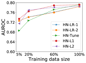
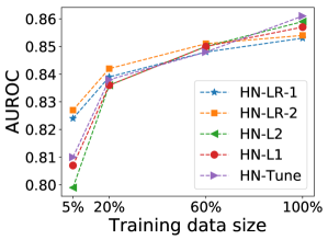
We refer to the fine-tuned model using $L_{1}$ regularizer as HN-L1, $L_{2}$ regularizer as HN-L2, without regularizer as HN-Tune, and LR model learned using HN features as HN-LR, and consider two baselines for comparison: 1) Logistic Regression (LR) using statistical features (including mean, standard deviation, etc.) from raw time series as used in Harutyunyan et al. (2017), 2) RNN classifier (RNN-C) learned using training data for the target task. To test the robustness of the models for small labeled training sets, we consider subsets of training and validation datasets, while the test set remains the same. Further, we also evaluate the relevance of layer-wise features $\mathbf{z}_{\tau,l}$ from the $L=2$ hidden layers of HealthNet. HN-LR-1 and HN-LR-2 refer to models trained using $\mathbf{z}_{\tau,2}$ (the topmost hidden layer only) and $\mathbf{z}_{\tau}=[\mathbf{z}_{\tau,1},\mathbf{z}_{\tau,2}]$ (from both hidden layers), respectively.

Table 3: Fraction of features with weight $\approx$ 0.

Task	LR	HN-LR-1	HN-LR-2
Phenotyping	0.902 $\pm$ 0.023	0.955 $\pm$ 0.020	0.974 $\pm$ 0.011
In-hospital mortality	0.917	0.787	0.867

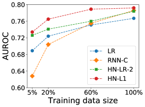
Comparison of HealthNet based transfer learning techniques: Phenotyping results in Figure 9(a) suggests that (i) all our proposed transfer learning approaches perform equally well when using 100% training data. (ii) regularized fine-tuned models (HN-L1 and HN-L2) consistently outperform non-regularized fine-tuned model (HN-Tune) as training dataset is reduced. As the size of labeled training set reduced, non-regularized fine-tuned model is prone to overfitting due to large number of trainable parameters. (iii) HN-L1 and HN-L2 outperform HN-LR model.

From Figure 9(b), we observe that (i) regularized fine-tuned models (HN-Tune, HN-L1, and HN-L2) perform comparable to HN-LR when training data is 100%. (ii) HN-LR consistently outperforms HN-Tune, HN-L1, and HN-L2 models as training dataset is reduced. This can be explained by the fact that the number of trainable parameters in HN-L1 and HN-L2 (of the order of square the number of hidden units) is significantly higher than the number of trianable parameters in HN-LR (of the order of number of hidden units), which is resulting in overfitting when labeled training dataset is very small.

Robustness to training data size: Phenotyping results in Figure 10(a) suggest that: (i) HN-L1 and RNN-C perform equally well when using 100% training data, and are better than LR. This implies that the transfer learning based models are as effective as models trained specifically for the target task on large labeled datasets. (ii) HN-L1 consistently outperforms RNN-C and LR models as training dataset is reduced. As the size of labeled training dataset reduces, the performance of RNN-C as well as HN-L1 degrades. However, importantly, we observe that HN-LR degrades more gracefully and performs better than RNN-C. The performance gains from transfer learning are greater when the training set of the target task is small. Therefore, with transfer learning, fewer labeled instances are needed to achieve the same level of performance as model trained on target data alone. (iii) As labeled training set is reduced, LR performs better than RNN-C confirming that deep networks are prone to overfitting on small datasets.

From Figure 10(b), we interestingly observe that HN-LR-2 results are at least as good as RNN-C and LR on the seemingly unrelated task of mortality prediction, suggesting that the features learned are generic enough and transfer well.

Importance of features from different hidden layers: We observe that HN-LR-1 and HN-LR-2 perform equally well for phenotyping task (Figure 9(a)), suggesting that adding features $\mathbf{z}_{\tau,1}$ from lower hidden layer do not improve the performance given higher layer features $\mathbf{z}_{\tau,2}$. For the mortality prediction task, we observe slight improvement in HN-LR-2 over HN-LR-1, i.e. adding lower layer features helps. A possible explanation for this behavior is as follows: since training was done on phenotyping tasks, features from top-most layer suffice for new phenotypes as well; on the other hand, the more generic features from the lower layer are useful for the unrelated task of mortality prediction.

Number of relevant features for a task: We observe that only a small number of features are actually relevant for a target classification task out of large number of input features to LR models (714 for LR, 300 for HN-LR-1, and 600 for HN-LR-2), As shown in Table 3, $>$95% of features have weight $\approx$ 0 (absolute value $<$ 0.001) for HN-LR models corresponding to phenotyping tasks due to sparsity constraint (eq. 6), i.e. most features do not contribute to the classification decision. The weights of features that are non-zero for at least one of target tasks for HN-LR-1 are shown in Supplementary Material Figure 12. We observe that, for example, for HN-LR-1 model only 130 features (out of 300) are relevant across the 10 phenotype classification tasks and the mortality prediction task. This suggests that HN provides several generic features while LR learns to select the most relevant ones given a small labeled dataset. Table 3 and Figure 12 also suggest that HN-LR models use larger number of features for mortality prediction task, possibly because concise features for mortality prediction are not available in the learned set of features as HN was pre-trained for phenotype identification tasks.

10 Conclusion

Deep neural networks require heavy computational resources for training and are prone to overfitting. Scarce labeled training data, significant hyper-parameter tuning efforts, and scarce computational resources are often a bottleneck in adopting deep learning based solutions to healthcare applications. In this work, we have proposed effective approaches for transfer learning in healthcare domain by using deep recurrent neural networks (RNN). We considered two scenarios for transfer learning: i) adapting a deep RNN-based universal time series feature extractor (TimeNet) to healthcare tasks and applications, and ii) adapting a deep RNN (HealthNet) pre-trained on healthcare tasks to a new related task. Our approach brings the advantage of deep learning such as automated feature extraction and ability to easily deal with variable length time series while still being simple to adapt to the target tasks. We have demonstrated that our transfer learning approaches can lead to significant gains in classification performance compared to traditional models using carefully designed statistical features or task-specific deep models in scarcely labeled training data scenarios. Further, leveraging pre-trained models ensures very little tuning effort, and therefore, fast adaptation. We also found that raw feature-wise handling of time series via TimeNet, and subsequent linear classifier training can provide insights into the importance and relevance of a raw feature (physiological parameter) for a given task while still modeling the temporal aspect. This raw feature relevance scoring can help domain-experts gain at least a high-level insight into the working of otherwise opaque deep RNNs.

In future, evaluating a domain-specific TimeNet-like model for clinical time series (e.g. trained only on MIMIC-III database) will be interesting. Also, transferability and generalization capability of RNNs trained simultaneously on diverse tasks (such as length of stay, mortality prediction, phenotyping, etc. Harutyunyan et al. (2017); Song et al. (2017)) to new tasks is an interesting future direction.

Conflict of interest

On behalf of all authors, the corresponding author states that there is no conflict of interest.

Supplementary Material

Appendix A Multilayered RNN with Gated Recurrent Units

A Gated Recurrent Unit (GRU) Cho et al. (2014) consists of an update gate and a reset gate that control the flow of information by manipulating the hidden state of the unit as in Equation 7.

In an RNN with $L$ hidden layers, the reset gate is used to compute a proposed value $\mathbf{\tilde{z}}_{t}^{l}$ for the hidden state $\mathbf{z}_{t}^{l}$ at time $t$ for the $l$-th hidden layer by using the hidden state $\mathbf{z}_{t-1}^{l}$ and the hidden state $\mathbf{z}_{t}^{l-1}$ of the units in the lower hidden layer at time $t$. The update gate decides as to what fractions of previous hidden state and proposed hidden state to use to obtain the updated hidden state at time $t$. In turn, the values of the reset gate and update gate themselves depend on the $\mathbf{z}_{t-1}^{l}$ and $\mathbf{z}_{t}^{l-1}$

We use dropout variant for RNNs as proposed in Pham et al. (2014) for regularization such that dropout is applied only to the non-recurrent connections, ensuring information flow across time-steps.

The time series goes through the following transformations iteratively for $t=1$ through $T$, where $T$ is length of the time series:

$$reset\,gate:\mathbf{r}_{t}^{l}=\sigma(\mathbf{W}_{r}^{l}\cdot\mathbf{D}(\mathbf{z}_{t}^{l-1}),\mathbf{z}_{t-1}^{l}])$$ (7)

$$update\,gate:\mathbf{u}_{t}^{l}=\sigma(\mathbf{W}_{u}^{l}\cdot[\mathbf{D}(\mathbf{z}_{t}^{l-1}),\mathbf{z}_{t-1}^{l}])$$

$$proposed\,state:\mathbf{\tilde{z}}_{t}^{l}=\tanh(\mathbf{W}_{p}^{l}\cdot[\mathbf{D}(\mathbf{z}_{t}^{l-1}),\mathbf{r}_{t}\odot\mathbf{z}_{t-1}^{l}])$$

$$hidden\,state:\mathbf{z}_{t}^{l}=(1-\mathbf{u}_{t}^{l})\odot\mathbf{z}_{t-1}^{l}+\mathbf{u}_{t}^{l}\odot\mathbf{\tilde{z}}_{t}^{l}$$

where $\odot$ is Hadamard product, $[\mathbf{a},\mathbf{b}]$ is concatenation of vectors $\mathbf{a}$ and $\mathbf{b}$, $\mathbf{D}(\cdot)$ is dropout operator that randomly sets the dimensions of its argument to zero with probability equal to dropout rate, $\mathbf{z}_{t}^{0}$ equals the input at time $t$. $\mathbf{W}_{r}$, $\mathbf{W}_{u}$, and $\mathbf{W}_{p}$ are weight matrices of appropriate dimensions s.t. $\mathbf{r}_{t}^{l},\mathbf{u}_{t}^{l},\mathbf{\tilde{z}}_{t}^{l}$, and $\mathbf{z}_{t}^{l}$ are vectors in $\mathbf{R}^{c^{l}}$, where $c^{l}$ is the number of units in layer $l$. The sigmoid ($\sigma$) and $tanh$ activation functions are applied element-wise.

Figure 11: Feature relevance scores for 25 phenotypes using TimeNet based transfer learning. Refer Table 4 for names of phenotypes, and Table 5 for names of raw features.

Figure 12: Feature weights (absolute) for HN-LR-1. Here P_i ($i=1,\ldots,10$) denotes $i$-th phenotype identification task. x-axis: Feature Number, y-axis: Task.

Table 4: Phenotype-wise Classification Performance in terms of AUROC.

90 S.No. Phenotype LSTM-Multi TimeNet-48 TimeNet-All TimeNet-48-Eps TimeNet-All-Eps 1 Acute and unspecified renal failure 0.8035 0.7861 0.7887 0.7912 0.7941 2 Acute cerebrovascular disease 0.9089 0.8989 0.9031 0.8986 0.9033 3 Acute myocardial infarction 0.7695 0.7501 0.7478 0.7533 0.7509 4 Cardiac dysrhythmias 0.684 0.6853 0.7005 0.7096 0.7239 5 Chronic kidney disease 0.7771 0.7764 0.7888 0.7960 0.8061 6 Chronic obstructive pulmonary disease and bronchiectasis 0.6786 0.7096 0.7236 0.7460 0.7605 7 Complications of surgical procedures or medical care 0.7176 0.7061 0.6998 0.7092 0.7029 8 Conduction disorders 0.726 0.7070 0.7111 0.7286 0.7324 9 Congestive heart failure; nonhypertensive 0.7608 0.7464 0.7541 0.7747 0.7805 10 Coronary atherosclerosis and other heart disease 0.7922 0.7764 0.7760 0.8007 0.8016 11 Diabetes mellitus with complications 0.8738 0.8748 0.8800 0.8856 0.8887 12 Diabetes mellitus without complication 0.7897 0.7749 0.7853 0.7904 0.8000 13 Disorders of lipid metabolism 0.7213 0.7055 0.7119 0.7217 0.7280 14 Essential hypertension 0.6779 0.6591 0.6650 0.6757 0.6825 15 Fluid and electrolyte disorders 0.7405 0.7351 0.7301 0.7377 0.7328 16 Gastrointestinal hemorrhage 0.7413 0.7364 0.7309 0.7386 0.7343 17 Hypertension with complications and secondary hypertension 0.76 0.7606 0.7700 0.7792 0.7871 18 Other liver diseases 0.7659 0.7358 0.7332 0.7573 0.7530 19 Other lower respiratory disease 0.688 0.6847 0.6897 0.6896 0.6922 20 Other upper respiratory disease 0.7599 0.7515 0.7565 0.7595 0.7530 21 Pleurisy; pneumothorax; pulmonary collapse 0.7027 0.6900 0.6882 0.6909 0.6997 22 Pneumonia 0.8082 0.7857 0.7916 0.7890 0.7943 23 Respiratory failure; insufficiency; arrest (adult) 0.9015 0.8815 0.8856 0.8834 0.8876 24 Septicemia (except in labor) 0.8426 0.8276 0.8140 0.8296 0.8165 25 Shock 0.876 0.8764 0.8564 0.8763 0.8562

Table 5: List of raw input features.

90 1 Glucose 31 Glascow coma scale eye opening $\rightarrow$ 3 To speech 2 Glascow coma scale total $\rightarrow$ 7 32 Height 3 Glascow coma scale verbal response $\rightarrow$ Incomprehensible sounds 33 Glascow coma scale motor response $\rightarrow$ 5 Localizes Pain 4 Diastolic blood pressure 34 Glascow coma scale total $\rightarrow$ 14 5 Weight 35 Fraction inspired oxygen 6 Glascow coma scale total $\rightarrow$ 8 36 Glascow coma scale total $\rightarrow$ 12 7 Glascow coma scale motor response $\rightarrow$ Obeys Commands 37 Glascow coma scale verbal response $\rightarrow$ Confused 8 Glascow coma scale eye opening $\rightarrow$ None 38 Glascow coma scale motor response $\rightarrow$ 1 No Response 9 Glascow coma scale eye opening $\rightarrow$ To Pain 39 Mean blood pressure 10 Glascow coma scale total $\rightarrow$ 6 40 Glascow coma scale total $\rightarrow$ 4 11 Glascow coma scale verbal response $\rightarrow$ 1.0 ET/Trach 41 Glascow coma scale eye opening $\rightarrow$ To Speech 12 Glascow coma scale total $\rightarrow$ 5 42 Glascow coma scale total $\rightarrow$ 15 13 Glascow coma scale verbal response $\rightarrow$ 5 Oriented 43 Glascow coma scale motor response $\rightarrow$ 4 Flex-withdraws 14 Glascow coma scale total $\rightarrow$ 3 44 Glascow coma scale motor response $\rightarrow$ No response 15 Glascow coma scale verbal response $\rightarrow$ No Response 45 Glascow coma scale eye opening $\rightarrow$ Spontaneously 16 Glascow coma scale motor response $\rightarrow$ 3 Abnorm flexion 46 Glascow coma scale verbal response $\rightarrow$ 4 Confused 17 Glascow coma scale verbal response $\rightarrow$ 3 Inapprop words 47 Capillary refill rate $\rightarrow$ 0.0 18 Capillary refill rate $\rightarrow$ 1.0 48 Glascow coma scale total $\rightarrow$ 13 19 Glascow coma scale verbal response $\rightarrow$ Inappropriate Words 49 Glascow coma scale eye opening $\rightarrow$ 1 No Response 20 Systolic blood pressure 50 Glascow coma scale motor response $\rightarrow$ Abnormal extension 21 Glascow coma scale motor response $\rightarrow$ Flex-withdraws 51 Glascow coma scale total $\rightarrow$ 11 22 Glascow coma scale total $\rightarrow$ 10 52 Glascow coma scale verbal response $\rightarrow$ 2 Incomp sounds 23 Glascow coma scale motor response $\rightarrow$ Obeys Commands 53 Glascow coma scale total $\rightarrow$ 9 24 Glascow coma scale verbal response $\rightarrow$ No Response-ETT 54 Glascow coma scale motor response $\rightarrow$ Abnormal Flexion 25 Glascow coma scale eye opening $\rightarrow$ 2 To pain 55 Glascow coma scale verbal response $\rightarrow$ 1 No Response 26 Heart Rate 56 Glascow coma scale motor response $\rightarrow$ 2 Abnorm extensn 27 Respiratory rate 57 pH 28 Glascow coma scale verbal response $\rightarrow$ Oriented 58 Glascow coma scale eye opening $\rightarrow$ 4 Spontaneously 29 Glascow coma scale motor response $\rightarrow$ Localizes Pain 59 Oxygen saturation 30 Temperature

References

- Bahdanau et al. (2014) Bahdanau D, Cho K, Bengio Y (2014) Neural machine translation by jointly learning to align and translate. arXiv preprint arXiv:14090473
- Bengio (2012) Bengio Y (2012) Deep learning of representations for unsupervised and transfer learning. In: Proceedings of ICML Workshop on Unsupervised and Transfer Learning, pp 17–36
- Che et al. (2016) Che Z, Purushotham S, Cho K, Sontag D, Liu Y (2016) Recurrent neural networks for multivariate time series with missing values. arXiv preprint arXiv:160601865
- Chen et al. (2015) Chen Y, Keogh E, Hu B, Begum N, et al. (2015) The ucr time series classification archive. www.cs.ucr.edu/~eamonn/time_series_data/
- Cho et al. (2014) Cho K, Van Merriënboer B, Gulcehre C, Bahdanau D, Bougares F, Schwenk H, Bengio Y (2014) Learning phrase representations using RNN encoder-decoder for statistical machine translation. arXiv preprint arXiv:14061078
- Choi et al. (2016) Choi E, Bahadori MT, Schuetz A, Stewart WF, Sun J (2016) Doctor ai: Predicting clinical events via recurrent neural networks. In: Machine Learning for Healthcare Conference, pp 301–318
- Gupta et al. (2018a) Gupta P, Malhotra P, Vig L, Shroff G (2018a) Transfer learning for clinical time series analysis using recurrent neural networks
- Gupta et al. (2018b) Gupta P, Malhotra P, Vig L, Shroff G (2018b) Using features from pre-trained timenet for clinical predictions
- Harutyunyan et al. (2017) Harutyunyan H, Khachatrian H, Kale DC, Galstyan A (2017) Multitask learning and benchmarking with clinical time series data. arXiv preprint arXiv:170307771
- Hermans and Schrauwen (2013) Hermans M, Schrauwen B (2013) Training and analysing deep recurrent neural networks. In: Advances in Neural Information Processing Systems, pp 190–198
- Hosmer Jr et al. (2013) Hosmer Jr DW, Lemeshow S, Sturdivant RX (2013) Applied logistic regression, vol 398. John Wiley & Sons
- Johnson et al. (2016) Johnson AE, Pollard TJ, et al. (2016) Mimic-iii, a freely accessible critical care database. Scientific data 3:160035
- Kingma and Ba (2014) Kingma DP, Ba J (2014) Adam: A method for stochastic optimization. arXiv preprint arXiv:14126980
- Lee et al. (2017) Lee JY, Dernoncourt F, Szolovits P (2017) Transfer learning for named-entity recognition with neural networks. arXiv preprint arXiv:170506273
- Lipton et al. (2015) Lipton ZC, Kale DC, Elkan C, Wetzel R (2015) Learning to diagnose with lstm recurrent neural networks. arXiv preprint arXiv:151103677
- Malhotra et al. (2015) Malhotra P, Vig L, Shroff G, Agarwal P (2015) Long Short Term Memory Networks for Anomaly Detection in Time Series. In: ESANN, 23rd European Symposium on Artificial Neural Networks, Computational Intelligence and Machine Learning, pp 89–94
- Malhotra et al. (2017) Malhotra P, TV V, Vig L, Agarwal P, Shroff G (2017) TimeNet: Pre-trained deep recurrent neural network for time series classification. In: 25th European Symposium on Artificial Neural Networks, Computational Intelligence and Machine Learning, pp 607–612
- Micenková et al. (2013) Micenková B, Dang XH, Assent I, Ng RT (2013) Explaining outliers by subspace separability. In: Data Mining (ICDM), 2013 IEEE 13th International Conference on, IEEE, pp 518–527
- Miotto et al. (2016) Miotto R, Li L, Kidd BA, Dudley JT (2016) Deep patient: an unsupervised representation to predict the future of patients from the electronic health records. Scientific reports 6:26094
- Miotto et al. (2017) Miotto R, Wang F, Wang S, Jiang X, Dudley JT (2017) Deep learning for healthcare: review, opportunities and challenges. Briefings in bioinformatics
- Nguyen et al. (2017) Nguyen P, Tran T, Wickramasinghe N, Venkatesh S (2017) Deepr: A convolutional net for medical records. IEEE journal of biomedical and health informatics 21(1):22–30
- Pan and Yang (2010) Pan SJ, Yang Q (2010) A survey on transfer learning. IEEE Transactions on knowledge and data engineering 22(10):1345–1359
- Pascanu et al. (2013) Pascanu R, Mikolov T, Bengio Y (2013) On the difficulty of training recurrent neural networks. arXiv preprint arXiv:12115063
- Pham et al. (2014) Pham V, Bluche T, Kermorvant C, Louradour J (2014) Dropout improves recurrent neural networks for handwriting recognition. In: Frontiers in Handwriting Recognition (ICFHR), IEEE, pp 285–290
- Purushotham et al. (2017) Purushotham S, Meng C, Che Z, Liu Y (2017) Benchmark of deep learning models on large healthcare mimic datasets. arXiv preprint arXiv:171008531
- Rajkomar et al. (2018) Rajkomar A, Oren E, Chen K, Dai AM, Hajaj N, Liu PJ, Liu X, Sun M, Sundberg P, Yee H, et al. (2018) Scalable and accurate deep learning for electronic health records. arXiv preprint arXiv:180107860
- Ravì et al. (2017) Ravì D, Wong C, Deligianni F, Berthelot M, Andreu-Perez J, Lo B, Yang GZ (2017) Deep learning for health informatics. IEEE journal of biomedical and health informatics 21(1):4–21
- Serra et al. (2018) Serra J, Pascual S, Karatzoglou A (2018) Towards a universal neural network encoder for time series
- Simonyan and Zisserman (2014) Simonyan K, Zisserman A (2014) Very deep convolutional networks for large-scale image recognition. arXiv preprint arXiv:14091556
- Song et al. (2017) Song H, Rajan D, Thiagarajan JJ, Spanias A (2017) Attend and diagnose: Clinical time series analysis using attention models. arXiv preprint arXiv:171103905
- Sutskever et al. (2014) Sutskever I, Vinyals O, Le QV (2014) Sequence to sequence learning with neural networks. In: Advances in Neural Information Processing Systems, pp 3104–3112
- Tibshirani (1996) Tibshirani R (1996) Regression shrinkage and selection via the lasso. Journal of the Royal Statistical Society Series B (Methodological) pp 267–288
- Yosinski et al. (2014) Yosinski J, Clune J, Bengio Y, Lipson H (2014) How transferable are features in deep neural networks? In: Advances in neural information processing systems, pp 3320–3328