Transit least-squares survey

We apply for the first time the Transit Least-Squares (TLS) algorithm to search for new transiting exoplanets. TLS has been developed as a successor to the Box Least-Squares (BLS) algorithm, which has served as a standard tool for the detection of periodic transits. In this proof-of-concept paper, we demonstrate how TLS finds small planets that have previously been missed. We showcase TLS’s capabilities using the K2 EVEREST-detrended light curve of the star K2-32 (EPIC 205071984), which has been known to have three transiting planets. TLS detects these known Neptune-sized planets K2-32 b, d, and c in an iterative search and finds an additional transit signal with a high signal detection efficiency (SDE_TLS) of 26.1 at a period of $4.34882_{-0.00075}^{+0.00069}$ d. We show that this additional signal remains detectable (SDE_TLS = 13.2) with TLS in the K2SFF light curve of K2-32, which includes a less optimal detrending of the systematic trends. The signal is below common detection thresholds, however, if searched with BLS in the K2SFF light curve (SDE_BLS = 8.9) as in previous searches. Markov Chain Monte Carlo sampling with the emcee software shows that the radius of this candidate is ${1.01}_{-0.09}^{+0.10}\,R_{\oplus}$. We analyze its phase-folded transit light curve using the vespa software and calculate a false positive probability ${\rm FPP}=3.1\leavevmode\nobreak\ \times\leavevmode\nobreak\ 10^{-3}$. Taking into account the multiplicity boost of the system, we estimate an ${\rm FPP}<3.1\leavevmode\nobreak\ \times\leavevmode\nobreak\ 10^{-4}$, which formally validates K2-32 e as a planet. K2-32 now hosts at least four planets that are very close to a 1:2:5:7 mean motion resonance chain. The offset of the orbital periods of K2-32 e and b from a 1:2 mean motion resonance is in very good agreement with the sample of transiting multiplanet systems from Kepler, lending further credence to the planetary nature of K2-32 e. We expect that TLS can find many more transits of Earth-sized and even smaller planets in the Kepler and K2 data that have hitherto remained undetected with algorithms that search for box-like signals.

1 Introduction

Figure 1: K2 light curve of K2-32. (a) After correction for systematic effects with EVEREST. The red line shows our running median filter. (b) Detrended light curve obtained by dividing the EVEREST light curve by the running median. Transits detected with TLS are highlighted with green (K2-32 b), magenta (K2-32 c), blue (K2-32 d), and stretched red (K2-32 e) vertical bars.

The data from the Kepler primary mission (K1; Borucki et al., 2010), which operated from 2009 to 2013, and from the repurposed K2 mission (Howell et al., 2014), which worked from 2014 to 2018, have both been subject to extensive transit searches. Most of their confirmed or validated planets (2338 from K1 and 359 from K2) and of the candidates that are yet to be confirmed (2423 from K1 and 536 from K2) have been found using the Box Least-Squares (BLS) transit search algorithm (Kovács et al., 2002) or similar algorithms searching for box-like flux decreases in stellar light curves (Batalha et al., 2013; Vanderburg et al., 2016; Crossfield et al., 2016, 2018; Mayo et al., 2018; Livingston et al., 2018b, a; Yu et al., 2018; van Sluijs & Van Eylen, 2018).

We developed the Transit Least-Squares (TLS) algorithm (Hippke & Heller, 2019) as the successor of BLS in order to be even more sensitive to smaller possibly sub-Earth-sized planets. Instead of searching for box-like flux decreases in the light curve, TLS is based on an analytical transit model with stellar limb darkening (Manduca et al., 1977; Mandel & Agol, 2002). The signal detection efficiency of TLS is consequently improved compared to BLS, while the false-positive rate is also suppressed (Hippke & Heller, 2019). Here we use TLS to search for so far unknown planets in the K2 data of K2-32 (EPIC 205071984), and we present our first discovery from our new data analysis campaign, the TLS Survey.

Three planets have previously been reported around K2-32 by Vanderburg et al. (2016), who formally designated them as candidates, and by Crossfield et al. (2016), who validated them as planets K2-32 b, c, and d using additional high-resolution spectroscopy and independent stellar photometry to feed the statistical vetting software vespa (Morton, 2012, 2015). Mayo et al. (2018), also using vespa and additional adaptive optics observations, again detected the three transiting objects and determined their probabilities of being an eclipsing binary, background eclipsing binary, or hierarchical eclipsing binary each to be $<10^{-4}$. Most important, all these previous detections of K2-32 b, c, and d were achieved in searches for box-like transit signals. Vanderburg et al. (2016) used BLS, Crossfield et al. (2016) used the TERRA software (Petigura et al., 2013a), which includes a search for box-like transit signals very much like BLS, and Mayo et al. (2018) also used BLS. K2-32 b, c, and d have also been confirmed through stellar radial velocity measurements by Dai et al. (2016) and Petigura et al. (2017).

Figure 2: Signal detection efficiencies of our successive transit search after masking out previously detected transits.

Figure 3: Phase-folded transit light curves of all planets. Dots show the K2 data, lines represent our best-fit MCMC models. The ordinates in the top and bottom panels have different scales. In the top panel, the transit dip of K2-32 e is shown together with a sliding mean (dashed line) of 11 cadences in width.

Figure 4: System architecture. Stellar and planetary radii are to scale. Planetary distances to the star are mutually to scale, but not with respect to the radii. The shapes of the transit light curves are to scale as well. Orbital resonances are indicated with respect to the innermost planet K2-32 e. The error bars denote our uncertainties in the transit impact parameter (Table 1).

Figure 5: Iterative transit search using K2SFF data with BLS (left) and TLS (right). Planets K2-32 b, d, and c are successively detected with strong signals (see labels) with both BLS and TLS. Using a common detection threshold value of 9, however, planet e is not detected with BLS (SDE_BLS = 8.9), but it is detected with TLS (SDE_TLS = 13.2). The major peak near $P=0.4$ d with (SDE_BLS = 10.5) in the fourth iteration of BLS is a false positive (blue marker). It overshadows the true transit signal near $P=4.3\,$d with (SDE_BLS = 8.9).

2 Methods

2.1 Target selection

In this paper, we move on from the testing phase of TLS (Hippke & Heller, 2019) and apply TLS to real light curves. In this initial phase of the TLS Survey, we restrict ourselves to multiplanet systems from the Kepler mission because they have been shown to exhibit extremely low false-positive probabilities (FPP) (Lissauer et al., 2012). Among the systems that we studied, K2-32 with its three previously known planets stood out with our detection of a highly significant fourth transit signal, the method of which we describe in the following.

2.2 Transit search

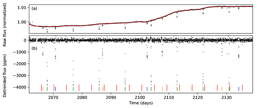
The light curve of K2-32 from campaign 2 contains 77.4 d of almost uninterrupted observations with 3527 useful exposures at a cadence of 30 min. We ignored the first 64 exposures in the light curve because they are affected by strong systematics. We removed outliers, defined as data points $>3\,\sigma$ above the running mean, from the publicly available K2 light curve of K2-32, which has been corrected for instrumental effects with EVEREST (Luger et al., 2016, 2018) (Fig. 1a). We then removed stellar variability and other trends using a median filter with a window size of 1 d. The resulting detrended light curve is shown in Fig. 1(b).

We tested other window sizes and found that a width of 1 d offers the best compromise between both sufficient removal of unwanted variability and preservation of transit signals with durations of up to several hours. Kepler’s third law of motion (Kepler, 1619) predicts that planets with orbital periods $<80\,$ d around sun-like stars have transit durations shorter than about 8 hr (see Fig. 5 in Hippke & Heller, 2019). For K2-32 in particular, the maximum duration of a planet with a single transit in the 80 d K2 light curve on a circular orbit is 5.7 hr, and for a planet to exhibit two transits (hence $P<40$ d) the maximum transit duration is 4.8 hr, suggesting that a 1 d width for our median filter hardly affects physically plausible transit signals.

We applied the publicly available python implementation of TLS (Hippke & Heller, 2019) using the stellar-limb darkening, mass, and radius estimates available from the EPIC catalog (Huber et al., 2016). We used TLS version 1.0.16 in its default parameterization, but set the maximum trial period equal to the length of the light curve in order to search for possible single transits.

2.3 Markov chain Monte Carlo analysis of the transits

To refine the planetary parameters we used the Markov chain Monte Carlo (MCMC) sampler emcee (Foreman-Mackey et al., 2013). As inputs to emcee, we provided the times of the mid-points of the first transit ($T_{0}$) and the orbital period ($P$) obtained with TLS for each planet. $P$, $T_{0}$, the planet-to-star radius ratio ($R_{\rm p}/R_{\rm s}$), and the transit impact parameter ($b$) served as model parameters for each planet, while the stellar density ($\rho_{\rm s}$) and two limb-darkening coefficients for a quadratic limb darkening law (Kipping, 2013) were global parameters for all transits. We ran the MCMC analysis with 100 walkers with each walker performing $200,000$ steps. The first half of each walk was discarded to ensure that we preserved only burned-in MCMC chains.

3 Results

Table 1: Characterization of the new planet K2-32 e from MCMC model fitting to the full set of transits in the EVEREST light curve of K2-32.

	Planet e		Planet b		Planet c		Planet d
	ML	median${}_{-{\rm err.}}^{+{\rm err.}}$	ML	median${}_{-{\rm err.}}^{+{\rm err.}}$	ML	median${}_{-{\rm err.}}^{+{\rm err.}}$	ML	median${}_{-{\rm err.}}^{+{\rm err.}}$
$P$ [d]	4.34911	$4.34882_{-0.00075}^{+0.00069}$	8.991866	$8.991828_{-0.000084}^{+0.000083}$	20.66157	$20.66186_{-0.00098}^{+0.00102}$	31.7145	$31.7142_{-0.0010}^{+0.0011}$
$T_{0}$ [d]	$0.8799$	$0.8860_{-0.0079}^{+0.0085}$	$2.92698$	$2.92713_{-0.00034}^{+0.00035}$	$1.4231$	$1.4227_{-0.0021}^{+0.0021}$	$5.7923$	$5.7913_{-0.0017}^{+0.0014}$
$R_{\rm p}/R_{\rm s}$	0.01080	$0.01090_{-0.00051}^{+0.00052}$	0.05347	$0.05382_{-0.00068}^{+0.00076}$	0.029430	$0.029664_{-0.00053}^{+0.00058}$	0.03534	$0.03551_{-0.00062}^{+0.00064}$
$b$	0.029	$0.22_{-0.15}^{+0.17}$	0.047	$0.15_{-0.10}^{+0.16}$	0.24	$0.28_{-0.08}^{+0.10}$	0.451	$0.463_{-0.030}^{+0.057}$

Table 2: System parameterization of K2-32 and its planets and comparison to literature values.

	Star	Planet e	Planet b	Planet c	Planet d	Ref.
$P$ [d]			$8.99213$	$20.6602$	$31.7154$	C16
			$8.99218_{-0.00020}^{+0.00020}$	$20.65614_{-0.00598}^{+0.00598}$	$31.71922_{-0.00236}^{+0.00236}$	D16
			$8.99213_{-0.00016}^{+0.00016}$	$20.6602_{-0.0017}^{+0.0017}$	$31.7154_{-0.0022}^{+0.0022}$	P17
			$8.99194_{-0.00016}^{+0.00016}$	$20.6616_{-0.0018}^{+0.0017}$	$31.7151_{-0.0026}^{+0.0022}$	M18
		$4.34882_{-0.00075}^{+0.00069}$	$8.991828_{-0.000084}^{+0.000083}$	$20.66186_{-0.00098}^{+0.00102}$	$31.7142_{-0.0010}^{+0.0011}$	H19
$R$			$5.62\,R_{\oplus}$	$3.32\,R_{\oplus}$	$3.77\,R_{\oplus}$	C16
	$0.87_{-0.05}^{+0.05}\,R_{\odot}$		$5.38_{-0.35}^{+0.35}\,R_{\oplus}$	$3.48_{-0.42}^{+0.97}\,R_{\oplus}$	$3.75_{-0.40}^{+0.40}\,R_{\oplus}$	D16
	$0.845_{-0.035}^{+0.044}\,R_{\odot}$		$5.13_{-0.28}^{+0.28}\,R_{\oplus}$	$3.01_{-0.25}^{+0.25}\,R_{\oplus}$	$3.43_{-0.35}^{+0.35}\,R_{\oplus}$	P17
	$0.839_{-0.026}^{+0.021}\,R_{\odot}$		$5.17_{-0.20}^{+0.16}\,R_{\oplus}$	$3.12_{-0.18}^{+0.12}\,R_{\oplus}$	$3.41_{-0.26}^{+0.14}\,R_{\oplus}$	M18
		$1.01_{-0.09}^{+0.10}\,R_{\oplus}$	$4.96_{-0.27}^{+0.33}\,R_{\oplus}$	$2.74_{-0.16}^{+0.20}\,R_{\oplus}$	$3.27_{-0.19}^{+0.23}\,R_{\oplus}$	H19
$M$	$0.87_{-0.04}^{+0.04}\,M_{\odot}$		$21.1_{-5.9}^{+5.9}\,M_{\oplus}$	$<8.1\,M_{\oplus}$ (95 % conf.)	$<35.0\,M_{\oplus}$ (95 % conf.)	D16
	$0.856_{-0.028}^{+0.028}\,M_{\odot}$		$16.5_{-2.7}^{+2.7}\,M_{\oplus}$	$<12.1\,M_{\oplus}$ (95 % conf.)	$10.3_{-4.7}^{+4.7}\,M_{\oplus}$	P17
$a$ [AU]			$0.0811$	$0.14120$	$0.1879$	C16
			$0.08036_{-0.00088}^{+0.00088}$	$0.1399_{-0.0015}^{+0.0015}$	$0.1862_{-0.0020}^{+0.0020}$	P17
		$0.04951_{-0.00055}^{+0.00055}$	$0.08035_{-0.00089}^{+0.00089}$	$0.1399_{-0.0016}^{+0.0016}$	$0.1862_{-0.0021}^{+0.0021}$	H19
FPP			$0$	$5\times 10^{-4}$	$5.4\times 10^{-6}$	C16
			$<1\times 10^{-3}$	$2.2\times 10^{-2}$	$<1\times 10^{-3}$	S16
			$<1\times 10^{-4}$	$<1\times 10^{-4}$	$<1\times 10^{-4}$	M18
		$3.1\times 10^{-3}$	$5.2\times 10^{-3}$	$4.9\times 10^{-3}$	$7.2\times 10^{-3}$	H19

3.1 Transit detection and characterization

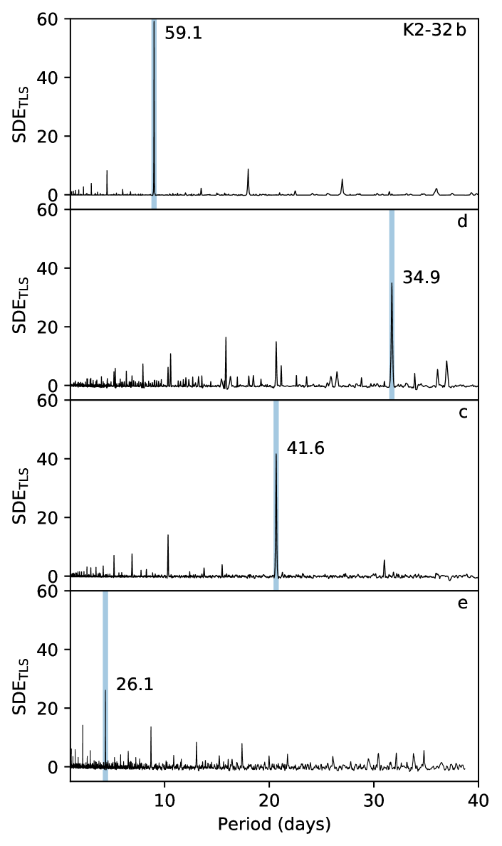
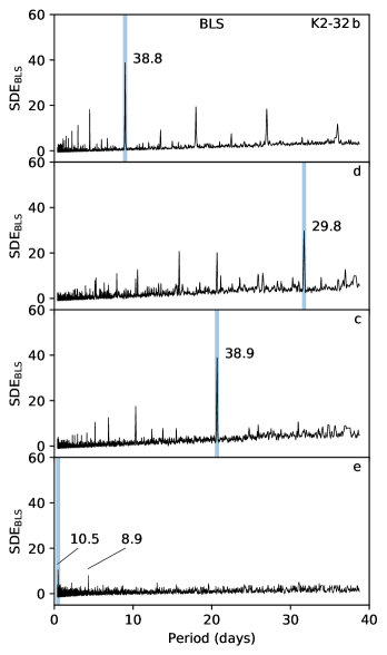
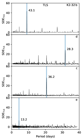
In Fig. 2 we show the signal detection efficiency (SDE_TLS) periodograms of our iterative transit search with TLS in the K2 light curve that has been extracted with EVEREST. Each iteration ignores the in-transit data corresponding to transits detected in previous iterations. TLS first found planet b (top panel) because it is both the largest planet and exhibits more transits than planets c and d in the light curve. Next, TLS found planet d (second panel), which is the second largest planet in the system. Planet c was detected in our third iteration with TLS (third panel). In a fourth run then, we found another strong peak (SDE_TLS = 26.1) at a period of $4.34882_{-0.00075}^{+0.00069}$ d, which we preliminary referred to as a candidate dubbed K2-32 e. We also executed a fifth search after masking out all transits from the four planets, but we did not find any other significant signals.

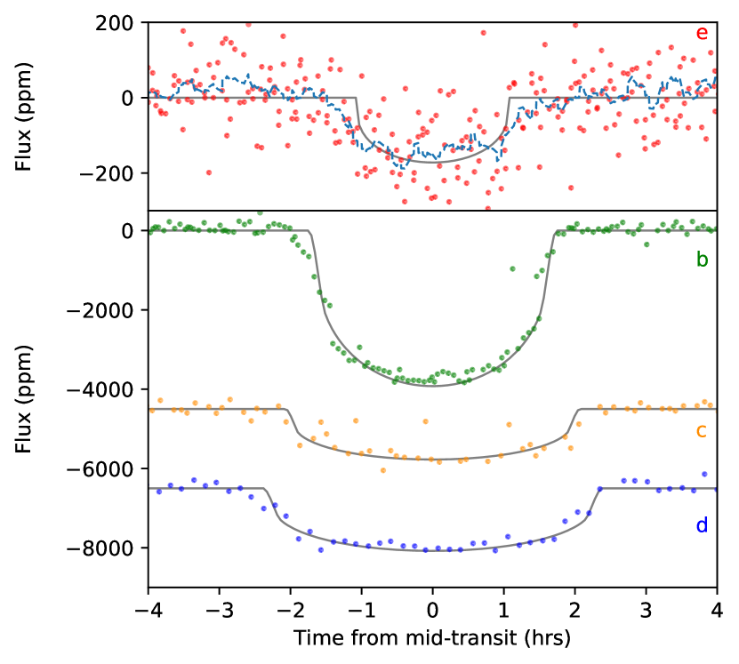
Figure 3 illustrates the phase-folded light curves of K2-32 e (top panel) and of the previously discovered planets b, c, and d from top to bottom. The shallow transit depth of about 200 parts per million (ppm) is immediately suggestive of an Earth-sized planet, given that K2-32 is a somewhat subsolar-sized K dwarf star. We note that the ordinate in the top panel, which shows the transit data of the new object, is an 18-fold zoom compared to the bottom panel, which contains the data of planets b, c, and d.

To further characterize the new planet candidate, we applied the MCMC sampler to the entire light curve. The stellar density was found to be $1.42_{-0.15}^{+0.08}$ times the solar density and the best-fit limb-darkening parameters are $q_{1}=0.57_{-0.18}^{+0.23}$ and $q_{2}=0.47_{-0.11}^{+0.16}$. Our results for K2-32 e are shown in Table 1, and our results from the MCMC sampling for the previously known planets K2-32 b, c, and d are compared to the literature values in Table 2.

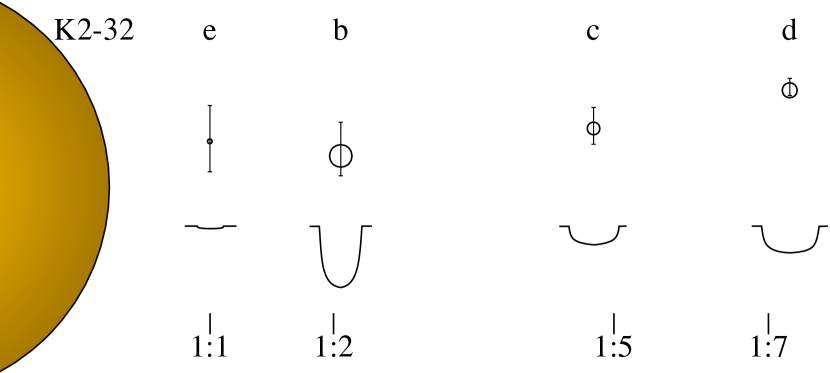
Figure 4 is a visualization of the physical and orbital characteristics. K2-32 is indicated as a cropped orange shaded circle, and its planets are denoted by empty circles with radii to scale with the star. The vertical bars denote the uncertainties in $b$, and the transit curves are to-scale representations of the best-fit transit models shown in Fig. 3. Orbital resonances are indicated at the bottom of this chart, with the 1:1 resonance referring to the innermost planet, K2-32 e. Interestingly, we found that this four-planet system is close to being in a 1:2:5:7 mean motion resonance (MMR) chain. At the same time, however, the system is clearly out of this resonance compared to our measurement uncertainties.

3.2 False-positive vetting and validation

We used the publicly available vespa software (Morton, 2012, 2015) to evaluate the FPP of K2-32 e. In brief, vespa takes the phase-folded transit light curve together with the celestial coordinates and stellar parameters to calculate the probabilities of the data being caused by non-associated blended eclipsing binaries, hierarchical triples, genuine eclipsing binaries, and non-associated stars with transiting planets. We supplied vespa with the celestial coordinates of K2-32, $P$ and $R_{\rm p}/R_{\rm s}$ of our candidate signal (Table 1), the phase-folded transit light curve (Fig 3, top panel), the stellar parameters as determined spectroscopically by Petigura et al. (2017) (Table 2), and the 2MASS broadband photometry ($J\leavevmode\nobreak\ =\leavevmode\nobreak\ 10.404\,\pm\,0.024$, $H=9.993\,\pm\,0.025$, $K=9.821\,\pm\,0.019$; Cutri et al., 2003) following the “Lessons Learned” section in Petigura et al. (2017). As a limiting aperture within which the transits are observed, we referred to adaptive optics and K2 light curve analyses of Sinukoff et al. (2016), who found that the transits are localized within 8 arcseconds of K2-32. vespa returned an FPP of $3.1\leavevmode\nobreak\ \times\leavevmode\nobreak\ 10^{-3}$ for K2-32 e.

Although this number formally validates K2-32 e as a planet already (the commonly used FFP threshold for validation is 1 %), it still does not consider the “multiplicity boost” (reduction in FPP) inherent to planet candidates in multiplanet systems. Planet candidates in systems known to already harbor planets have a much lower FPP than single candidates (Lissauer et al., 2012). We used the values of the homogeneous K2 exoplanet survey by Vanderburg et al. (2016) with $n_{\rm t}=59{,}174$ as the number of target stars (K2 campaigns 0 to 3), $n_{\rm c}=234$ as the number of K2 planet candidates, and $n_{\rm m}=26$ as the number of candidate multiplanet systems and plugged them into Eq. (6) of Lissauer et al. (2012). We found that the total number (the expectation value) of K2 systems like K2-32 with two or more known planets and one additional false positive ranges between 0.01, assuming a true-positive rate (or planet fidelity) of 90 %, and 0.05, assuming a true-positive rate of 50 %. These estimates increased our confidence that K2-32 e is a true planet because both values are much lower than 1. Sinukoff et al. (2016) showed that based on the statistical framework of Lissauer et al. (2012), the multiplicity boost is at least an order of magnitude in FPP. As a consequence, a conservative estimate of the FPP for K2-32 e including the multiplicity boost is $<\,3.1\times 10^{-4}$.

With the depth of the secondary transit ($\delta_{2}$) being of the order of $(R_{\rm p}/a)^{2}$, or 0.056 ppm in the case of K2-32 e, we expect this phenomenon to be invisible to K2. Thus, as an additional test for a false positive, for example, caused by an eclipsing binary, we measured $\delta_{2}$ in that part of the light curve where the secondary transit can be expected on a circular orbit. We detected a $8\pm 8\,$ppm dip, that is to say, a $1\,\sigma$ signal that is statistically compatible with noise.

3.3 Comparison of the BLS and TLS performances

One of the most pressing questions is why K2-32 e has not been detected in previous transit searches, for instance, those by Vanderburg et al. (2016) and Crossfield et al. (2016).

For our comparison of the transit search results obtained with BLS and TLS, we have to keep in mind that the definitions of the signal detection efficiency introduced by Kovács et al. (2002) for BLS (SDE_BLS) and by Hippke & Heller (2019) for TLS (SDE_TLS) are different. While SDE_BLS is more closely related to the mean transit depth, SDE_TLS is derived from a $\chi^{2}$ statistic and therefore naturally tends to produce higher values for a given transit-like signal. This principal difference between SDE_BLS and SDE_TLS must also be noted in the context of the heuristically chosen detection thresholds of typically between 8 and 9 in other studies. We have shown in Hippke & Heller (2019), using injected transits of Earth-like planets in the light curves of Sun-like stars with white noise, that a false-positive rate of 1 % is achieved at virtually the same signal detection efficiency value of 7 for both BLS (here SDE${}_{\rm BLS}=7$) and TLS (here SDE${}_{\rm TLS}=7$). Although the statistics of BLS and TLS are different, they produced the same SDE values for this particular set of simulated data. Most important, however, the true-positive rates were $\sim\leavevmode\nobreak\ 76$ % for BLS and $\sim\leavevmode\nobreak\ 93$ % for TLS. The TERRA algorithm uses yet another search statistic, the signal-to-noise ratio (S/N) with a detection threshold set to a nominal value of 12 “by trial and error” (Petigura et al., 2013b).

Vanderburg et al. (2016) and Crossfield et al. (2016) both used the K2 light curve produced with the “K2 self-flat-fielding” (K2SFF) pipeline, which removes most of the instrumental jitter (Vanderburg & Johnson, 2014). This light curve contains a somewhat stronger noise than the light curve extracted with the EVEREST pipeline, and we therefore need to examine whether our discovery of K2-32 e is owing to improvements of the K2 light curve extraction and systematic detrending or due to the use of TLS instead of BLS. We thus repeated our analysis using the K2SFF data and tested both TLS and BLS, the results of which are shown in Fig. 5.

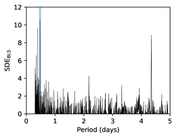
In the left column of Fig. 5, we present an iterative transit search in the K2SFF light of K2-32 with BLS. We successively detected planets b, d, and c with very strong SDE_BLS signals (see labels) whereas planet e produced an SDE_BLS of just 8.9 in the fourth iteration, which is below the widely used detection threshold value of 9 (Vanderburg et al., 2016; Crossfield et al., 2016). We verified that the addition of a smoothing filter to the SDE_BLS spectrum, similar to what is done in TLS to the SDE_TLS spectrum, does not lift this signal above the detection threshold. None of the previous K2 transit surveys by Vanderburg et al. (2016), Crossfield et al. (2016), Petigura et al. (2018), and Mayo et al. (2018) applied such a smoothing filter to their SDE_BLS or S/N spectra.

Moreover, the signature of K2-32 e is only the second strongest signal, while the strongest signal near $P=0.4\,$d with an SDE_BLS of 10.5 is a false positive, as we verified. We found that this false-positive signal is produced by a combination of two characteristics of BLS; the quantification in transit durations in units of cadences and the linear period grid typically used in BLS applications. For example, Petigura et al. (2013b) used “transit durations that are integer numbers of long cadence measurements (…)” with a grid of, for example, “$\Delta T=[3,5,7,10,14,18]$ long cadence measurements.” Aliasing effects of duration and period integer multiples cause additional jitter in the BLS spectrum, an effect that is absent in TLS because it does not apply any binning. In addition, the period grid in TLS is not linear (Ofir, 2014) because the frequency grid is linear, which intrinsically suppresses the possibility of aliasing.

We are therefore able to reproduce the results of previous searches with the traditional BLS algorithm and confirm that K2-32 e remains undetected in the K2SFF light curve.

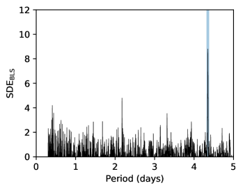
In the right column of Fig. 5, we show the SDE_TLS results for an iterative transit search with TLS in the K2SFF data. We found planets b, d, and c with SDE_TLS values comparable to those obtained with BLS, but most interestingly planet e also passed the detection limit with a significant SDE_TLS of 13.2. This is a fascinating real-world example of the simulation-based findings by Hippke & Heller (2019): the strongest improvement in using TLS instead of BLS occurs for shallow transits or, in this case, for Earth-sized planets.

We also found that planet e can be recovered in the EVEREST data with both BLS (SDE_BLS = 21.3) and TLS (SDE_TLS = 26.1). We conclude that if either the TLS search algorithm or the EVEREST data reduction pipeline would have been available to Vanderburg et al. (2016) and Crossfield et al. (2016), they could have found K2-32 e. Most important, however, the combination of EVEREST and TLS leverages the optimal detrending and signal detection procedures.

We also examined the different methods that were used to remove longer-term stellar trends. Vanderburg et al. (2016) and Crossfield et al. (2016) both used spline fits, while we used a running median by default. When we used a spline fit instead of a running median, the SDE_TLS values obtained with TLS were virtually identical with variations of about 0.1.

4 Discussion

4.1 K2-32 system

Figure 6: Left: Zoom into the bottom left panel of Fig. 5. The major peak near $P=0.4$ d (blue marker) in the SDE_BLS spectrum is a false positive that is caused by an aliasing effect of the discrete cadence-based duration grid employed by most BLS implementations, here using $10,000$ trial periods on a linear grid between 0.3 d and 5 d. Right: Same as in the left panel but now using more than ten times as many trial periods and a nonlinear period grid with the spacing increasing as $P^{1/3}$. Although the false positive peak near $P=0.4$ d has disappeared, the signal of K2-32 e near $P=4.3$ d is still formally a false negative with SDE${}_{\rm BLS}=8.9$.

For now, the mass of K2-32 e remains unconstrained. With one Earth radius in size, a first guess for the mass of K2-32 e is about one Earth mass. Although the densities of planets b, c, and d range between those of Saturn and Neptune, which suggests large and massive gaseous envelopes, it can safely be assumed that K2-32 e does not carry large amounts of gas. If K2-32 e consisted mostly of gas, its low density would imply a sub-Earth-mass planet. Such a very low-mass (and very low-gravity) planet, however, could hardly hold on to a significant gas envelope, in particular under the effects of extreme stellar irradiation. Assuming an Earth-mass ($M_{\oplus}$) for K2-32 e, a nominal stellar mass of $0.856\,M_{\odot}$, and a semimajor axis of 0.04951 AU (Table 2), we estimate a stellar radial velocity (RV) amplitude of $0.44\,{\rm m\,s}^{-1}$, which seems just beyond the reach of modern spectrographs (Dai et al., 2016; Petigura et al., 2017). Even if K2-32 e were made up fully of iron, its mass of then roughly $1.4\,M_{\oplus}$ would imply an RV amplitude of just about $0.6\,{\rm m\,s}^{-1}$ and hardly surpass the RV noise (or RV jitter) of several m s^-1 that is typical for solar-type main-sequence stars (Wright, 2005)

We also studied whether transit timing variations (TTVs) could be an alternative avenue to determine the planetary masses around K2-32 (Holman & Murray, 2005; Agol et al., 2005). Using our MCMC characterization of the system (Table 1), a mass of $16.5\,M_{\oplus}$ for planet K2-32 b (Petigura et al., 2017), and a nominal Earth mass for K2-32 e, we find that Eq. (8) from Lithwick et al. (2012) predicts a TTV amplitude of $\sim 140$ s or 0.04 hr for K2-32 e. This is probably undetectable in the available Kepler data (see top panel of Fig. 3) but could be tested in a detailed follow-up study.

The near 1:2:5:7 MMR chain of K2-32 e that we report is somewhat reminiscent of other MMR chains, such as the 3:4:6:8 MMR chain observed in the Kepler-223 system (Mills et al., 2016). While the Kepler-223 system exhibits a very precise MMR tuning that has been interpreted as a footprint of planet migration, the fact that K2-32 is substantially non-synchronized with the 1:2:5:7 MMR chain suggests that additional processes have been at work. The origin of these deviations from precise commensurability might be in long-term star-planet tidal interaction that was only overruled by the MMR-creating effects of the protoplanetary disk in the very early stages of the system (Papaloizou, 2011; Heller, 2018). K2-32 joins the family of planetary systems from the Kepler mission that are just wide of exact commensurability (Lee et al., 2013), although K2-32 represents a particular case with four rather than just two near-resonant planets. Lissauer et al. (2011) defined a new variable

$$\zeta_{1}=3\left(\frac{1}{\mathcal{P}-1}-{\rm Round}{\Big{(}}\frac{1}{\mathcal{P}-1}{\Big{)}}\right)$$ (1)

as a measure of the difference between an observed first-order MMR period ratio, where $\mathcal{P}=P_{\rm o}/P_{\rm i}$ is the orbital period ratio between the outer and the inner planet. These authors found statistically significant deviations of the observed $\zeta_{1}$ distribution from a random period ratio distribution for about 100 transiting exoplanets from Kepler known at the time. Their results showed that for a randomly drawn pair of Kepler planets, $\zeta$ is most likely to range between -0.1 and -0.2. Taking the median orbital periods from our MCMC sampling for K2-32 e and b (Table 1), which are very close to the 2:1 MMR resonance ($P_{\rm o}/P_{\rm i}=2.0676$), we find $\zeta_{1}=-0.19$. Although this result cannot be used as a means of verification for K2-32 e, it is in very good agreement with a large sample of exoplanets from Kepler (Lissauer et al., 2011) and, therefore serves as an indirect piece of evidence in favor of the planetary nature of K2-32 e.

4.2 Aliasing effects in BLS

Figure 5 shows the results we obtained with the BLS reference implementation in astropy. Nevertheless, the question arises if the occurrence of a false positive near $P=0.4$ d could be avoided with different grids for the trial periods and trial durations. We therefore varied the resolution and spacing of both the duration and the period grids for BLS to determine whether we could remove this alias peak. The results are illustrated in Fig. 6 and are discussed in the following.

First, the grid of trial transit durations used in BLS must be in multiples of a constant cadence. As an intrinsic property of BLS, any given cadence is tested for one of two test flux values that relate to either the out-of-transit flux or to the in-transit flux (Kovács et al., 2002). As a consequence, when BLS is applied with a period grid of constant spacing, short trial periods may happen to be integer multiples of the trial duration. For example, a trial period of 0.416 d is sufficiently close to the $20$-fold multiple of a 30 min trial transit duration (a single long-cadence exposure of a K2 light curve), and a 10-fold multiple of a 60 min transit duration (worth two cadences), etc. As the transit duration grows with the orbital period to the power of one-third (Eq. (10) in Hippke & Heller, 2019), everything else being equal, aliasing becomes less of an issue for longer trial periods. Nevertheless, aliasing cannot be avoided completely by using an infinitely fine period grid. Instead, it can be avoided by using a nonlinear period grid as employed by TLS.

Second, the grid of trial durations tested with BLS is usually the same for all trial periods, see, for example, the BLS implementation in astropy. Although users can define a maximum trial duration of, for example, $\sim 0.21\,$days (or 10 cadences), which is sufficiently long for most long-period planets in K2, this trial duration is as much as half of an orbital period for the most short-period planets that are physically plausible. Again, clustering of data can generate aliases such as those visible near $P=0.3$ d in Fig. 6 (left panel) and eventually lead to false-positive detections. In this example, the most reliable way for us to remove the alias peaks was to use a hyperfine nonlinear grid of $>100,000$ trial periods in combination with a duration grid that uses a maximum trial duration shorter than half of the shortest period. Nevertheless, and maybe most important, the signal of K2-32 e near $P=4.3$ d remained a false negative for the BLS search.

In practice, it could be possible to develop more appropriate trial period and trial duration grids for BLS similar to the grid that is implemented in TLS, but this is beyond the scope of this paper and the disadvantage of the suboptimal detector shape (box versus limb-darkened transit) would remain.

5 Conclusions

We determined with high significance (SDE_TLS = 26.1) a fourth sequence of periodic transits in the light curve of K2-32. Our MCMC simulations suggest that this signal has a period of $4.34882_{-0.00075}^{+0.00069}$ d and the transiting planet has a radius of ${1.01}_{-0.09}^{+0.10}\,R_{\oplus}$, making it one of the smallest planets found with K2 so far. Our false-positive vetting of K2-32 e as an individual transiting object yields ${\rm FPP}=3.1\times 10^{-3}$. Factoring in the planetary multiplicity around K2-32, we find ${\rm FPP}<3.1\times 10^{-4}$. This formally validates K2-32 e as a planet.

This new planet reveals a near 1:2:5:7 MMR chain of now four planets around K2-32. While being very close to this MMR chain, however, the planets are in fact just wide of exact commensurability, thereby joining a growing family of this type of systems from the Kepler mission. We find that the offset from exact commensurability between the new planet and the previously know K2-32 b is in very good agreement with the offsets found in other multiplanet transiting systems, adding more evidence in favor of the planetary nature of K2-32 e. K2-32 also joins the list of K2 systems with four or more transiting planet candidates, about a dozen of which are known as of today. For now, K2-138 is the only system with five (Christiansen et al., 2018) or potentially even six (Hardegree-Ullman & Christiansen, 2019) transiting planets, all of which are in the super-Earth to sub-Neptune radius regime.

Our discovery confirms that TLS can find sub-Earth-sized planets that have previously been missed with search algorithms looking for box-like transit signals such as BLS (Kovács et al., 2002). We verified that there are two reasons why previous searches have missed K2-32 e. First, we used the K2 light curve of K2-32 that was subject to the highly efficient removal of systematic effects with EVEREST (Luger et al., 2016), while previous searches used the light curve detrended with K2SFF that has slightly less favorable noise properties. Second, TLS is intrinsically more efficient in finding shallow transits because the search function is a transit and not a box (Hippke & Heller, 2019). Interestingly, we find that K2-32 e could have been detected in the K2SFF light curve with TLS.