Exclusion in Junction Geometries

Abstract

We investigate the dynamics of the asymmetric exclusion process at a junction. When two input roads are initially fully occupied and a single output road is initially empty, the ensuing rarefaction wave has a rich spatial structure. The density profile also changes dramatically as the initial densities are varied. Related phenomenology arises when one road feeds into two. Finally, we determine the phase diagram of the open system, where particles are fed into two roads at rate $\alpha$ for each road, the two roads merge into one, and particles are extracted from the single output road at rate $\beta$.

I Introduction

In exclusion processes, sites can be occupied by at most one particle and particles hop to empty sites. This paradigmatic model sheds much light on non-equilibrium steady states, large deviations, and other aspects of strongly-interacting infinite-particle systems (see, e.g., Spohn91 ; SZ95 ; D98 ; S00 ; BE07 ; D07 ; book and references therein). The totally asymmetric simple exclusion process (TASEP), where particles can hop to neighboring empty sites in one direction, is a minimalist realization of exclusion processes that is particularly tractable and also has a diverse range of applications MGP68 ; CSS00 ; CMZ11 ; AES15 .

In this work, we investigate the properties of the TASEP at a junction, where a small number of incoming roads, that each carry a TASEP, meet at a single point and particles leave via an outgoing road (or roads) also by the TASEP (Fig. 1). Our initial motivation came from the observation of maddening delays that arise when disembarking from a passenger plane. Here, the aisle(s) get clogged with passengers who are either slow in retrieving their belongings or in walking, leading to a clogging at the exit door of the plane. Our junction TASEP model is a rough caricature for this disembarkment process. We study in detail (Sec. III) the $(2,1)$ junction geometry with two roads that start at $x=-\infty$ and merge at $x=0$ into a single outgoing road that extends to $x=+\infty$. We also analyze the $(1,2)$ junction geometry (Sec. IV) and finite systems (Sec. V). Our analysis can be generalized to other junction geometries.

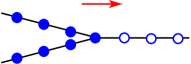
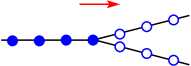
Figure 1: Illustration of the TASEP at: (a) a $(2,1)$ junction and (b) a $(1,2)$ junction. Shown is the downstep initial condition in which sites are fully occupied for $x<0$ (solid circles) and empty otherwise (open circles).

For the $(2,1)$ junction geometry, one might expect a pileup of particles as the junction is approached, reminiscent of what occurs when highway traffic approaches a lane constriction. The role of blockage in the TASEP has been considered previously in a one-dimensional geometry in which the hopping rate of a single bond is reduced from 1 to $r<1$ JL92 ; JL94 ; SPS15 . For the slow bond problem, particles jam upstream from the blockage, as one might anticipate, and the focus of JL92 ; JL94 ; SPS15 was to characterize this jam (see also Refs. K00 ; B06 ; CLST13 for reviews of this problem). A complementary TASEP model, in which particles may fly to any empty site when they reach a single special site was introduced in ABKM13 . All these studies focused on stationary properties. The slow bond problem with the domain wall initial condition was studied in L99 ; BSS14 ; BSS17 . A related line of research has focused on the role of an intersection on the TASEP, with the same number of incoming and outgoing roads at a junction N93 ; IF96 ; FSS04 ; FN07 ; BF08 ; EPK09 ; JA12 ; RPK13 ; Refs. EPK09 ; RPK13 study aspects of the TASEP in the junction geometries similar to those considered in our work.

In what follows, we assume that the hopping rates at each site are the same in all roads, and set them equal to 1. Thus each particle can hop to the right only if its right neighbor is empty. We define the location of the junction as the origin. We employ a hydrodynamic description and use the continuous density $\rho(x,t)$ as the basic dynamical variable in the long-time limit.

For the “downstep” initial condition in the $(2,1)$ junction geometry, in which each site on the two incoming roads are initially occupied while the single outgoing road is empty, the density profile at long times contains both a constant-density jammed segment upstream from the junction, as well as a downstream linear rarefaction wave (Fig. 2). As the initial density in the incoming roads is decreased, the form of the rarefaction wave changes dramatically and a shock wave can even arise. Similarly rich phenomenology arises for the $(1,2)$ junction geometry. Finally, we study the open $(2,1)$ system in which current is fed in to the system at rate $\alpha$ at each upstream road far from the junction and current is extracted at rate $\beta$ in the single road far downstream from the junction. We map out the phase diagram of this system and highlight the differences with the open TASEP system on the line.

II Shock and Rarefaction Waves

As a preliminary, we recapitulate the well-known (see, e.g., book ) density profile that arises in the TASEP on the line for the initial density step

$$\rho=\begin{cases}\rho_{\scriptstyle L}&x<0\,,\\[2.84526pt] \rho_{\scriptstyle R}&x>0\,,\end{cases}$$ (1)

where $\rho_{\scriptstyle L}$ and $\rho_{\scriptstyle R}$ are constant densities to the left and to the right of the step. The hydrodynamic behavior is governed by the continuity equation

$$\frac{\partial\rho}{\partial t}+\frac{\partial j}{\partial x}=0\,,$$ (2)

with the current given by $j=\rho(1-\rho)$. The solution to Eq. (2) subject to (1) has a remarkably simple scaling form

$$\rho(x,t)=f(z),\quad z=x/t\,.$$ (3)

When this scaling form is substituted into (2), two distinct behaviors arise that depend on whether $\rho_{\scriptstyle L}>\rho_{\scriptstyle R}$ or $\rho_{\scriptstyle L}<\rho_{\scriptstyle R}$:

• Rarefaction wave ($\rho_{\scriptstyle L}>\rho_{\scriptstyle R}$). An initial downstep relaxes to the rarefaction wave

  $$\rho(x,t)=\begin{cases}\rho_{\scriptstyle L}&z<1\!-\!2\rho_{\scriptstyle L}\,,\\[4.2679pt] \frac{1}{2}(1-z)&1\!-\!2\rho_{\scriptstyle L}<z<1\!-\!2\rho_{\scriptstyle R}\,,\\[4.2679pt] \rho_{\scriptstyle R}&z>1\!-\!2\rho_{\scriptstyle R}\,.\end{cases}$$ (4a)

• Shock wave ($\rho_{\scriptstyle L}<\rho_{\scriptstyle R}$). An upstep persists as a shock wave and merely translates:

  $$\rho(x,t)=\begin{cases}\rho_{\scriptstyle L}&z<c\,,\\[2.84526pt] \rho_{\scriptstyle R}&z>c\,,\end{cases}$$ (4b)

  with shock speed $c=1-\rho_{\scriptstyle R}-\rho_{\scriptstyle L}$.

III Rarefaction at a (2,1) Junction

We now investigate the evolution of the initial density step (1) at a junction where two roads merge into one. Here, and in the following section, the system is unbounded, with the incoming road(s) extending to $x=-\infty$ and the outgoing road(s) extending to $x=+\infty$. For simplicity, we treat the special case where the outgoing road is empty, $\rho_{\scriptstyle R}=0$, and where the initial densities in the incoming roads are both equal to $\rho_{\scriptstyle L}$. Three distinct behaviors arise for: (a) $\rho_{\scriptstyle L}>\rho_{+}$, (b) $\rho_{+}>\rho_{\scriptstyle L}>\rho_{-}$, and (c) $\rho_{\scriptstyle L}<\rho_{-}$, where $\rho_{+}$ and $\rho_{-}$ are critical densities whose values are given in Eq. (6) below. We discuss these three cases in turn.

III.1 High input density: $\rho_{\scriptstyle L}\geq\rho_{+}$

As in the conventional TASEP, a density downstep develops into a rarefaction wave in the subrange $0<x<t$. However, for $\rho_{\scriptstyle L}\geq\rho_{+}$, a density pileup develops just upstream from the junction, with a sudden density drop at $x=0$ (Fig. 2). This same qualitative behavior occurs as long as the initial input density $\rho_{\scriptstyle L}$ is greater than $\rho_{+}$. Upstream from the pileup, the density profile is again given the the classic rarefaction wave.

This rich behavior can be readily understood in the hydrodynamic limit. Substituting the scaling form (3) into the continuity equation (2) shows that the scaling function satisfies

$$f^{\prime}(z)\big{[}1-2f(z)-z\big{]}=0\,,$$ (5)

where the prime denotes differentiation with respect to $z$. The only solutions to this equation are either:

$$\text{flat\ profile}\quad\qquad f^{\prime}(z)=0,$$

$$\text{linear\ profile}\quad\quad f=\tfrac{1}{2}(1-z).$$

Any solution is a combination of these elemental forms. For the conventional TASEP, the solutions are the aforementioned rarefaction and shock wave solutions, Eqs. (4a)–(4b). To determine the rarefaction wave at a $(2,1)$ junction, note that the current just to the right of the junction cannot exceed the maximum possible value of $j_{\rm max}=\frac{1}{4}$. If one starts at $z=-1$ (equivalently $x=-t$), and increases $z$, the density decays from +1 as $\rho(z)=\frac{1}{2}(1-z)$. Correspondingly, the current increases as $j(z)=2\rho(1-\rho)=2\times\frac{1}{4}(1-z^{2})$, where the prefactor 2 accounts for the two upstream roads. Because the current cannot exceed $\frac{1}{4}$, $j(z)$ must “stick” at this value when first reached, which happens when $z=-1/\sqrt{2}$. Thus for $z$ in the range $-1/\sqrt{2}<z<0$, the density also sticks at a pileup value that corresponds to this maximal current. This maximal current condition is $2\rho(1-\rho)=\frac{1}{4}$, with solutions

$$\rho_{+}=\frac{1}{2}+\frac{1}{\sqrt{8}}\,,\qquad\rho_{-}=\frac{1}{2}-\frac{1}{\sqrt{8}}\,.$$ (6)

It is the larger root $\rho_{+}\approx 0.853553$ that is realized for the downstep initial condition, as shown in Fig. 2.

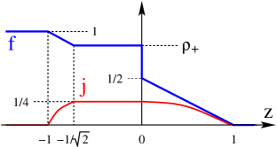
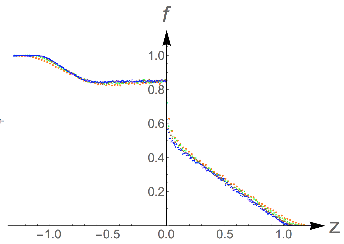
Figure 2: (a) Schematic, but to scale, scaled density profile for a rarefaction wave (blue) at a $(2,1)$ junction for an initial density downstep with $\rho_{\scriptstyle L}=1$. The corresponding current is shown in red. (b) Simulation data for the scaled density profile for this same initial condition for $t=125$ (red), $250$, (green) $500$ (brown), and $1000$ (blue).

For $z=0^{+}$, there is only a single road and the density must suddenly drop to $\frac{1}{2}$, so that the current at $z=0^{+}$ matches the maximal current $j_{\rm max}=\frac{1}{4}$ at $z=0^{-}$. For $0<z<1$, the density decays linearly with $z$ until the density reaches 0 at $z=1$. Thus in the high-density regime defined by $\rho_{\scriptstyle L}\geq\rho_{+}$, we conclude that the scaled density profile consists of five distinct segments:

$$f=\begin{cases}\rho_{\scriptstyle L}&\quad z<1-2\rho_{\scriptstyle L}\\[2.84526pt] \frac{1}{2}(1-z)&\quad 1-2\rho_{\scriptstyle L}<z<-\frac{1}{\sqrt{2}}\\[2.84526pt] \rho_{+}&\quad-\frac{1}{\sqrt{2}}<z<0\\[2.84526pt] \frac{1}{2}(1-z)&\quad 0<z<1\\[2.84526pt] 0&\quad z>1.\end{cases}$$ (7)

Simulation data converge to this five-segment form, with finite-time corrections that systematically vanish as $t$ increases (Fig. 2(b)). For the step initial condition, the system length is effectively infinite because the spatial range over which the density is varying is less than the actual system length.

III.2 Intermediate input density: $\rho_{-}\leq\rho_{\scriptstyle L}\leq\rho_{+}$

Distinct behavior arises when $\rho_{\scriptstyle L}$ lies between the two critical values $\rho_{+}$ and $\rho_{-}$. For $\rho_{\scriptstyle L}$ in this range, the current in each incoming road is less than $j_{\rm max}$, but the sum of the currents in the two roads exceeds $j_{\rm max}$. Thus there again must be a pileup of particles upstream from the junction point, as the maximum current that can be transmitted at the junction is $j_{\rm max}=\frac{1}{4}$. To match the outgoing current at the junction, the pileup density must equal $\rho_{+}$. On the other hand, the asymptotic density for $z\to-\infty$ is $\rho_{\scriptstyle L}$. As a result, a shock wave must arise whose speed is given by $1-\rho_{+}-\rho_{L}$. Thus when $\rho_{-}<\rho_{\scriptstyle L}<\rho_{+}$, the asymptotic density profile consists of four segments:

$$f=\begin{cases}\rho_{\scriptstyle L}&\quad z<1-\rho_{+}-\rho_{\scriptstyle L}\\ \rho_{+}&\quad 1-\rho_{+}-\rho_{\scriptstyle L}<z<0\\ \frac{1}{2}(1-z)&\quad 0<z<1\\ 0&\quad z>1\,.\end{cases}$$ (8)

Even though this initial density downstep leads to a rarefaction wave in the classic TASEP, the road constriction leads to a jam the manifests itself as a left-moving shock wave on the upstream side of the junction. A typical example profile for the case of $\rho_{\scriptstyle L}=2/3$ is shown in Fig. 3.

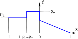
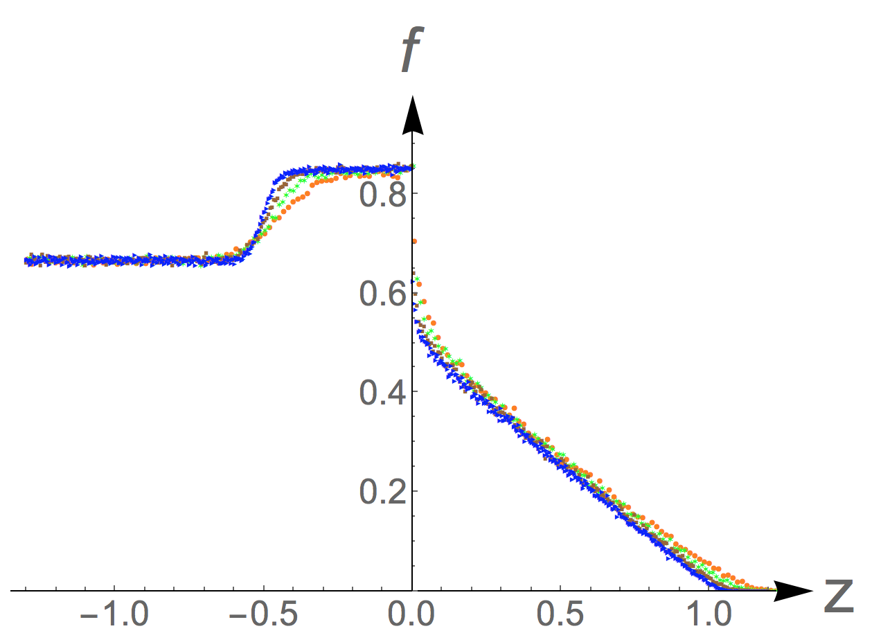
Figure 3: (a) The scaled density profile in Eq. (8) for the $(2,1)$ junction with $\rho_{\scriptstyle L}=2/3$. (b) Simulation data for this same initial condition for $t=125$ (red dots), $250$ (green), $500$ (brown), and $1000$ (blue). The linear rise in the density near $z=1-\rho_{\scriptstyle L}-\rho_{+}$ gradually steepens for increasing $t$, showing that this behavior is a finite-size effect.

III.3 Low input density: $\rho_{\scriptstyle L}\leq\rho_{-}$

Finally, we treat the low input density regime, where the incoming density obeys $\rho_{\scriptstyle L}\leq\rho_{-}$. Now the total current in the two incoming roads is always less than or equal to $j_{\rm max}=\frac{1}{4}$. Consequently, all the incoming current can be accommodated by the single output road. Therefore, there is no pileup at $x=0$ and the density profile in the incoming roads does not change in time.

In the special case of $\rho_{\scriptstyle L}=\rho_{-}$, the total input current to the junction equals $j_{\rm max}=\frac{1}{4}$, corresponding to the maximum current that can be accommodated by the output road. Here, the density profile for $z>0$ is again the classic rarefaction wave. When $\rho_{\scriptstyle L}<\rho_{-}$, the input current to the junction, $2\rho_{\scriptstyle L}(1-\rho_{\scriptstyle L})$, is less than $j_{\rm max}$. To have a consistent scaling solution for $z>0$, there must be a flat profile immediately to the right of the junction, with density $\rho_{\scriptstyle R}$, that eventually joins to the rarefaction wave $\rho(z)=\frac{1}{2}(1-z)$. We determine the density in the flat region to the right of the junction by matching the input and outgoing currents at $z=0$. This yields

$$j_{\rm in}=2\rho_{\scriptstyle L}(1-\rho_{\scriptstyle L})=\rho_{\scriptstyle R}(1-\rho_{\scriptstyle R})$$ (9a)

from which

$$\rho_{\scriptstyle R}=\frac{1-\sqrt{1-8\rho_{\scriptstyle L}(1-\rho_{\scriptstyle L})}}{2}\,.$$ (9b)

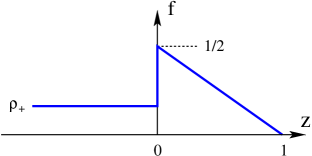
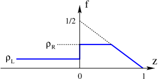
Figure 4: The scaled density profile for: (a) $\rho_{\scriptstyle L}=\rho_{-}\approx 0.146$ and $\rho_{\scriptstyle L}=\frac{1}{10}$.

Assembling these results, the scaled density profile consists of three segments when $\rho_{\scriptstyle L}=\rho_{+}$ (Fig. 4(a)):

$$f=\begin{cases}\rho_{\scriptstyle L}&\quad z<0\\ \frac{1}{2}(1-z)&\quad 0<z<1\\ 0&\quad z>1\,,\end{cases}$$ (10a)

and four segments for $$\rho_{\scriptstyle L}<\rho_{+}$$ (Fig. 4(b)):

$$f=\begin{cases}\rho_{\scriptstyle L}&\quad z<0\\ \rho_{\scriptstyle R}&\quad 0<z<1-2\rho_{\scriptstyle R}\\ \frac{1}{2}(1-z)&\quad 1-2\rho_{\scriptstyle R}<z<1\\ 0&\quad z>1\,.\end{cases}$$ (10b)

IV Rarefaction at a (1,2) Junction

The same type of arguments as those given above can be applied to the $(1,2)$ junction (see Fig. 1(b)). It is again natural to consider the initial condition of $\rho=\rho_{\scriptstyle L}$ for $z<0$ and $\rho=0$ for $z>0$ and study the behavior as a function of $\rho_{\scriptstyle L}$. As in the $(2,1)$ junction, a rich set of behaviors arises for varying $\rho_{\scriptstyle L}$ (Fig. 5).

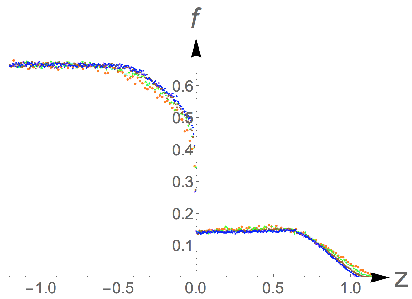
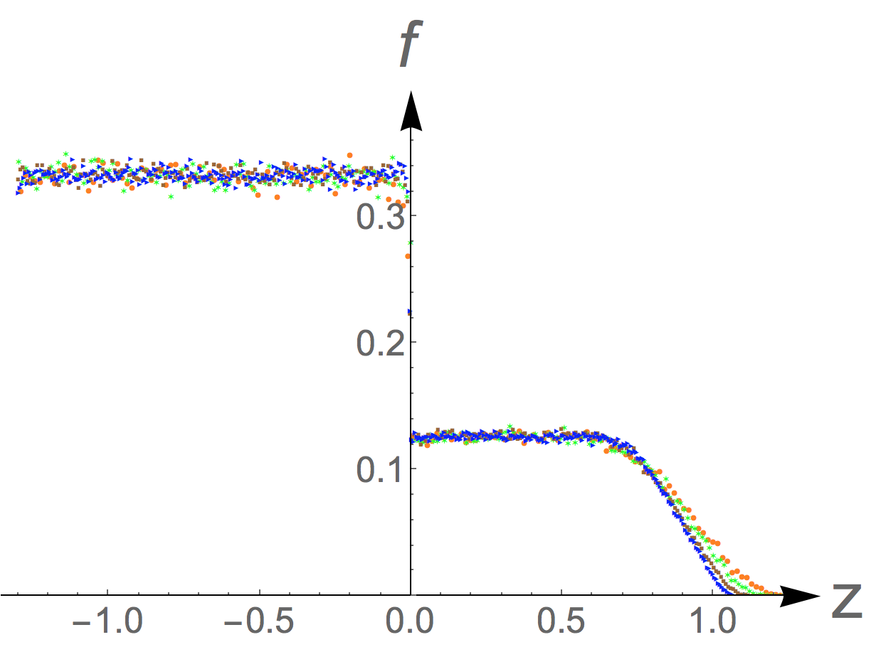
Figure 5: Simulation data for the density profile for the $(1,2)$ junction, for (a) $\rho_{\scriptstyle L}=2/3$ and (b) $\rho_{\scriptstyle L}=1/3$ for $t=125$ (red dots), 250 (green), 500 (brown), and 1000 (blue).

For the initial state where $\rho_{\scriptstyle L}=1$, that is, the input road is fully occupied and the two downstream roads are empty, we can exploit particle-hole duality of the TASEP to immediately infer the density profile. In this duality, a particle moving to the right corresponds to a hole (a vacancy) moving to the left. The density of holes $\rho_{h}$ is related to the particle density $\rho$ by $\rho_{h}=1-\rho$. Thus the dynamics of a right-moving TASEP at a $(1,2)$ junction with the downstep initial state of $\rho=1$ for $z<0$ and $\rho=0$ for $z>0$ is equivalent to the TASEP dynamics of holes that move to the left in the $(2,1)$ junction geometry with $\rho_{h}=1$ for $z>0$ and $\rho_{h}=0$ for $z<0$. The latter is the same as the particle density profile in a right-moving TASEP at a $(2,1)$ junction, after making the replacements $\rho\to 1-\rho$ and $z\to-z$. Simulations show that the density profile in this case is the mirror image of the density profile in Fig. 2(b)

An input density $\rho_{\scriptstyle L}<1$ in the $(1,2)$ junction geometry corresponds to a $(2,1)$ junction with density $\rho=1$ for $z<0$ and $\rho=1-\rho_{\scriptstyle L}$ for $z>0$; this correspondence is obvious after making the replacements $\rho\to 1-\rho$ and $z\to-z$. It is simpler to describe the dynamics in terms of a right-moving TASEP at a $(2,1)$ junction with the initial condition of $\rho=1$ for $z<0$ and $\rho=\rho_{\scriptstyle R}>0$ for $z>0$ and we do so in what follows.

For $t>0$, the density upstream from the junction again exhibits a pileup, in which the scaled profile $f=1$ for $z<-1$, $f=\frac{1}{2}(1-z)$ for $-1<z<-1/\sqrt{2}$, and finally $f=\rho_{+}$ for $-1/\sqrt{2}<z<0$. For $\rho_{\scriptstyle R}<\frac{1}{2}$, the incoming current equals its maximum value of $\frac{1}{4}$. This incoming current can be accommodated by a rarefaction wave for $z>0$ that ends when the density decays to $\rho_{\scriptstyle R}$. On the other hand, for $\rho_{\scriptstyle R}>\frac{1}{2}$, the outgoing current is density limited and, therefore equal to $j_{\scriptstyle R}=\rho_{\scriptstyle R}(1-\rho_{\scriptstyle R})$. This means that the pileup density $\rho_{\scriptstyle L}$ at $z=0^{-}$ is determined by matching the currents at $z=0$. This matching gives $2\rho_{\scriptstyle L}(1-\rho_{\scriptstyle L})=j_{\scriptstyle R}$, or $\rho_{\scriptstyle L}=\frac{1}{2}(1+\sqrt{1-2j_{\scriptstyle R}})$, in agreement with the density profile shown in Fig. 5(b).

V Open (2,1) Junction Geometry

We now study the $(2,1)$ junction with open boundary conditions with input rate $\alpha$ and output rate $\beta$. When the leftmost sites of the system are empty, particles are inserted with rate $\alpha$; one could consider distinct rates $\alpha_{1}$ and $\alpha_{2}$ for the two roads, but we limit ourselves to the symmetric case of $\alpha_{1}=\alpha_{2}=\alpha$. Similarly, when a particle reaches the rightmost site, it is extracted with rate $\beta$. These rates may take arbitrary positive values, but we limit ourselves to the range $0<\alpha<1$ and $0<\beta<1$. This restriction corresponds to the system being coupled to reservoirs with particle density $\alpha$ on the left and density $1-\beta$ on the right.

The behavior of this open system can be analyzed using the so-called domain wall theory Krug91 ; KS2 ; Krug01 ; SA02 ; Sch03 ; the basic predictions of this theory agree with exact analyses (see BE07 ; Sch03 for reviews). To put our results in context, it is helpful to first summarize the properties of an open single-road TASEP. Here, there are three phases (Fig: 6): (i) a low-density (LD) phase, when $\alpha<\frac{1}{2}$ and $\alpha<\beta$; (ii) a high-density (HD) phase, when $\beta>\frac{1}{2}$ and $\alpha>\beta$; (iii) a maximal-current (MC) phase, when $\alpha,\beta>\frac{1}{2}$. For the $(2,1)$ junction, the same three phases arise, but the locations of the phase boundaries are different than in a single-road system. The new feature for the $(2,1)$ junction geometry, which already arose in the closed system, is that current conservation at the junction leads to distinct densities just to the left and to the right of the junction.

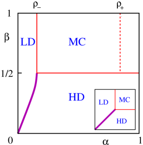
Figure 6: Phase diagram for the open $(2,1)$ junction. Inside the MC phase, $\alpha>\rho_{-}$ and $\beta>\frac{1}{2}$, the dashed vertical line at $\alpha=\rho_{+}$ separates a regime where the incoming road density is low, $\rho_{\scriptstyle L}=\rho_{-}$ when $\alpha<\rho_{+}$, from a high-density regime, $\rho_{\scriptstyle L}=\rho_{+}$ when $\alpha>\rho_{+}$. The inset shows the corresponding phase diagram for the open single-road system.

LD Phase: $\alpha<\rho_{-}$ and $\beta>\rho_{\scriptstyle R}(\alpha)$. In the low-density phase, the exit rate $\beta$ is relatively fast and the particle density is limited by the rate at which particles enter the system. Thus the density for $z<0$ is $\rho_{\scriptstyle L}=\alpha$. This statement holds as long as $\alpha<\rho_{-}$, so that the current is less than $\frac{1}{4}$. In this case, the right-half of the system can support and transmit this incoming current. Using the current conservation statement (9a) across the junction, as well as $\rho_{\scriptstyle L}=\alpha$, we immediately obtain, for the density in the right half of the system,

$$\rho_{\scriptstyle R}(\alpha)=\tfrac{1}{2}\left[1-\sqrt{1-8\alpha(1-\alpha)}\right]\,.$$ (11a)

The current in this LD phase is $$j(\alpha)=2\alpha(1-\alpha)$$.

HD Phase: $\alpha>\rho_{\scriptstyle L}(\beta)$ and $\beta<\frac{1}{2}$. In the high-density phase, the exit rate $\beta$ is relatively slow and the particle density is determined by the rate at which particles enter the system. In this HD phase, the density for $z>0$ is $\rho_{\scriptstyle R}=\beta$. We again invoke the current conservation statement (9a) across the junction and now solve for $\rho_{\scriptstyle L}$ to give

$$\rho_{\scriptstyle L}(\beta)=\tfrac{1}{2}\left[1-\sqrt{1-2\beta(1-\beta)}\right]\,.$$ (11b)

The current in this HD phase is $j(\beta)=\beta(1-\beta)$.

MC phase: $\alpha>\rho_{-}$ and $\beta>\frac{1}{2}$. The density before the junction in the MC phase is

$$\rho_{\scriptstyle L}=\begin{cases}\rho_{-}&\text{when}~{}~{}\rho_{-}<\alpha<\rho_{+}\\ \rho_{+}&\text{when}~{}~{}\rho_{+}<\alpha\end{cases}$$ (12)

The density in the two input roads can be either $\rho_{-}$ or $\rho_{+}$ to ensure that the total incoming current is the maximal possible current in a single road. Interestingly, the density in the left half of the system changes discontinuously when the input rate $\alpha=\rho_{+}$. For both cases the density in the right half of the system is $\rho_{\scriptstyle R}=\frac{1}{2}$ and the current is $j=\frac{1}{4}$ (see Fig. 7).

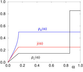
Figure 7: The bulk densities $\rho_{\scriptstyle L}(\alpha),\rho_{\scriptstyle R}(\alpha)$, and the current $j(\alpha)$ when $\beta>\frac{1}{2}$.

Coexistence line: The co-existence line is defined by the condition $\rho_{\scriptstyle R}(\alpha)=\beta$, with $\rho_{\scriptstyle R}(\alpha)$ given by Eq. (11), or equivalently $\rho_{\scriptstyle L}(\beta)=\alpha$, with $\rho_{\scriptstyle L}(\alpha)$ given by Eq. (11b). The additional conditions $\alpha<\rho_{-}$ and $\beta<\frac{1}{2}$ must also hold. This line (magenta in Fig. 6) separates the LD and HD phases. In the case of the single-road TASEP, subtle behaviors occur on the co-existence line $0<\alpha=\beta<\frac{1}{2}$. It is known KS2 that the density profile is a stationary shock wave with $\rho=\alpha$ near the left end and $\rho=1-\alpha$ near the right end. The location of the shock is a uniformly distributed random variable. By averaging over all possible locations of the shock for the open system on the interval $-L<x<L$, the density is given by

$$\rho(x)=\frac{1}{2}+\left(\frac{1}{2}-\alpha\right)\frac{x}{L}\,.$$ (13)

We anticipate a similar behavior on the co-existence line for the $(2,1)$ junction. The density near the entrance is $\alpha$ and the density near the exit is $1-\beta$. In the simplest situation when the shock is located at the junction

$$\rho=\begin{cases}\alpha&\quad-L_{1}<x<0\\ 1-\beta&~{}\qquad 0<x<L_{2}\,.\end{cases}$$ (14)

However, the distribution of the position of the shock front is unknown, and the lengths $L_{1}$ and $L_{2}$ of the incoming and outgoing roads may play a significant role.

VI Discussion

We introduced a simple extension of the totally asymmetric simple exclusion process (TASEP), in which multiple roads meet at a junction. We focused on two simple geometries, namely the $(2,1)$ and the $(1,2)$ junctions, in which either two roads merge into one, or one road splits into two. We first treated the density downstep initial condition, which normally leads to a rarefaction wave. For the $(2,1)$ junction geometry, we found much richer behavior in which there can be a particle pileup upstream from the junction. Additionally a shock wave can arise for a suitable range of initial densities. These phenomena qualitatively resemble what occurs in real traffic that approaches a constriction on a highway.

We also investigated non-equilibrium steady states in the $(2,1)$ junction with open boundaries in which particles are continuously fed in at the left end and removed from the right end. We analyzed this system using domain-wall theory Krug91 ; KS2 ; Krug01 ; SA02 ; Sch03 , which is known to correctly predict the phase diagram for the TASEP and more complicated lattice gases. It would be desirable to study junctions with open boundaries using exact approaches. One possibility is to attempt to extend the matrix product approach DEHP to the junction geometry. If the matrix product formulation can be extended to the junction geometry, then it should be feasible to provide detailed insights into the spatial structure of the non-equilibrium steady states. For example, the matrix product approach should be able to give the behavior of the density profile in the boundary layers near the left and right ends of the system, and in the inner layer near the junction. In the single-lane TASEP, these boundary layers exhibit qualitative changes within the low-density and high-density phases: the LD phase may be subdivided into LD-I and LD-II, and similarly for the HD phase. A more accurate description of the open $(2,1)$ junction phase diagram may perhaps be richer still due to the potentially different behaviors in the inner layer on either side of the junction.

Apart from generalizations to the $(m,n)$ junction geometry and to models with different hopping rates in the incoming and outgoing roads (which could be viewed as different speed limits in the two types of roads), one can probe the influence of the coupling between the parallel lanes in the bulk, in addition to the local interaction at the junction site. Multilane models can exhibit rich behaviors even without junctions (see, e.g., PS04 ; RJ07 ; EKST ; AES15 ). Junction-like geometries have been recently investigated in modeling pedestrian traffic Apper11 ; Apper13 ; however, the movement rules in these pedestrian movement models were significantly different from TASEP dynamics.

It would be also interesting to study the TASEP on more complicated graphs with vertices mimicking junctions. One amusing example is the TASEP on a figure-eight geometry, in which a particle can pass through the junction of the figure eight only when it is clear. This geometry is inspired by the infamous automobile races on the Islip Figure-Eight Speedway islip that were held between 1962 and 1984. The course is in the shape of a figure eight, with a collision point where the two loops of the figure eight meet. In this figure-eight geometry, we anticipate large collision-induced temporal fluctuations in the current passing through the junction.

Finally we emphasize that our analysis of junction geometries relied on hydrodynamic techniques, which yield only average characteristics. Fluctuations in the TASEP have attracted considerable interest. For example, for the density downstep initial condition, the total number of particles $N(t)$ that flow to the initially empty half-line by time $t$ is a random quantity whose fluctuations scale as $t^{1/3}$; that is,

$$N(t)=\tfrac{1}{4}\,t+t^{1/3}\xi\,.$$ (15)

The distribution $P(\xi)$ of the random variable $\xi$ was established by Johansson Johan . Remarkably, the same and related Tracy-Widom distributions were derived earlier in the context of random matrices TW94 , and they arise in a wider range of problems (see spohn ; Ivan_rev and references therein). For the $(2,1)$ junction we anticipate the same functional form (15), but the distribution of the corresponding random variable is unknown. For the $(1,2)$ junction, we expect that the total numbers of particles in each of the the two roads are

$$N_{1}(t)=\tfrac{1}{8}\,t+t^{1/3}\eta_{1},\quad N_{2}(t)=\tfrac{1}{8}\,t+t^{1/3}\eta_{2}\,.$$ (16)

The random variables $\eta_{1}$ and $\eta_{2}$ are correlated, and computing the joint distribution $P(\eta_{1},\eta_{2})$ appears to be challenging.

- (1) H. Spohn, Large Scale Dynamics of Interacting Particles (New York: Springer-Verlag, 1991).
- (2) B. Schmittmann and R. K. P. Zia, in Phase Transitions and Critical Phenomena, Vol. 17, eds. C. Domb and J. L. Lebowitz (Academic Press, London, 1995).
- (3) B. Derrida, Phys. Report 301, 65 (1998).
- (4) G. M. Schütz, “Exactly Solvable Models for Many-Body Systems Far From Equilibrium”, in Phase Transitions and Critical Phenomena, Vol. 19, eds. C. Domb and J. L. Lebowitz (Academic Press, London, 2000).
- (5) R. A. Blythe and M. R. Evans, J. Phys. A 40, R333 (2007).
- (6) B. Derrida, J. Stat. Mech. P07023 (2007).
- (7) P. L. Krapivsky, S. Redner, and E. Ben-Naim, A Kinetic View of Statistical Physics (Cambridge University Press, Cambridge, 2010).
- (8) C. MacDonald, J. Gibbs, and A. Pipkin, Biopolymers 6, 1 (1968).
- (9) D. Chowdhury, L. Santen, and A. Schadschneider, Phys. Repts. 329, 199 (2000).
- (10) T. Chou, K. Mallick, and R. K. P. Zia, Repts. Prog. Phys. 74, 116601 (2011).
- (11) C. Appert-Rolland, M. Ebbinghaus, and L. Santen, Phys. Repts. 593, 1 (2015).
- (12) S. A. Janowsky and J. L. Lebowitz, Phys. Rev. A 45, 618 (1992).
- (13) S. A. Janowsky and J. L. Lebowitz, J. Stat. Phys. 77, 35 (1994).
- (14) J. Schmidt, V. Popkov, and A. Schadschneider, Europhys. Lett. 110, 20008 (2015).
- (15) J. Krug, Braz. J. Phys. 30, 97 (2000).
- (16) M. Barma, Physica A 372, 22 (2006).
- (17) O. Costin, J. L. Lebowitz, E. R. Speer, and A. Troiani, Bull. Inst. Math. Acad. Sin. (N.S.)8, 49 (2013).
- (18) C. Arita, J. Bouttier, P. L. Krapivsky, and K. Mallick, Phys. Rev. E 88, 042120 (2013).
- (19) T. M. Liggett, Stochastic Interacting Systems: Contact, Voter and Exclusion Processes (Springer-Verlag, New York, 1985).
- (20) R. Basu, V. Sidoravicius, and A. Sly, arXiv:1408.3464.
- (21) R. Basu, V. Sidoravicius, and A. Sly, arXiv:1704.07799.
- (22) T. Nagatani, J. Phys. A 26, 6625 (1993).
- (23) Y. Ishibashi and M. Fukui, J. Phys. Soc. Jpn. 65, 2793 (1996).
- (24) M. Foulaadvand, Z. Sadjadi, and M. Shaebani, J. Phys. A 37, 561 (2004).
- (25) M. Foulaadvand and M. Neek-Amal, Europhys. Lett. 80, 60002 (2007).
- (26) S. Belbasi and M. E. Foulaadvand, J. Stat. Mech. P07021 (2008).
- (27) B. Embley, A. Parmeggiani, and N. Kern, Phys. Rev. E 80, 041128 (2009).
- (28) H. J. Hilhorst and C. Appert-Rolland, J. Stat. Mech. P06009 (2012).
- (29) A. Raguin, A. Parmeggiani, and N. Kern, Phys. Rev. E 88, 042104 (2013).
- (30) J. Krug, Phys. Rev. Lett. 67, 1882 (1991).
- (31) A. B. Kolomeisky, G. M. Schütz, E. B. Kolomeisky, and J. P. Straley, J. Phys. A 31, 6911 (1998).
- (32) J. S. Hager, J. Krug, V. Popkov, and G. M. Schütz, Phys. Rev. E 63, 056110 (2001).
- (33) L. Santen and C. Appert, J. Stat. Phys. 106, 187 (2001).
- (34) G. M. Schütz, J. Phys. A 36, R339 (2003).
- (35) B. Derrida, M. R. Evans, V. Hakim, and V. Pasquier, J. Phys. A 26, 1493 (1993).
- (36) V. Popkov and M. Salerno, Phys. Rev. E 69, 046103 (2004).
- (37) R. Juhász, Phys. Rev. E 76, 021117 (2007).
- (38) M. R. Evans, Y. Kafri, K. E. P. Sugden, and J. Tailleur, J. Stat. Mech. P06009 (2011).
- (39) C. Appert-Rolland, J. Cividini, and H. J. Hilhorst, J. Stat. Mech. P10014 (2011).
- (40) J. Cividini, H. J. Hilhorst, and C. Appert-Rolland, J. Phys. A 46, 345002 (2013).
- (41) https://en.wikipedia.org/wiki/Islip_Speedway.
- (42) K. Johansson, Commun. Math. Phys. 209, 437 (2000).
- (43) C. A. Tracy and H. Widom, Commun. Math. Phys. 159, 151 (1994); Commun. Math. Phys. 177, 727 (1996).
- (44) M. Prähofer and H. Spohn, “Current fluctuations for the totally asymmetric exclusion process,” pp. 185–204 in: In and Out of Equilibrium: Probability with a Physics Flavor, ed. by V. Sidoravicius (Birkäuser, Boston, 2006).
- (45) I. Corwin, Random Matrices Theory Appl. 1, 1130001 (2012).