Elaboration Tolerant Representation of Markov Decision Process via Decision-Theoretic Extension of Probabilistic Action Language $p{\cal BC}+$

Abstract

We extend probabilistic action language $p{\cal BC}+$ with the notion of utility in decision theory. The semantics of the extended $p{\cal BC}+$ can be defined as a shorthand notation for a decision-theoretic extension of the probabilistic answer set programming language ${\rm LP}^{\rm{MLN}}$. Alternatively, the semantics of $p{\cal BC}+$ can also be defined in terms of Markov Decision Process (MDP), which in turn allows for representing MDP in a succinct and elaboration tolerant way as well as leveraging an MDP solver to compute a $p{\cal BC}+$ action description. The idea led to the design of the system pbcplus2mdp, which can find an optimal policy of a $p{\cal BC}+$ action description using an MDP solver. This paper is under consideration in Theory and Practice of Logic Programming (TPLP).

1 Introduction

Many problems in Artificial Intelligence are about making decisions on actions to take. The chosen actions should maximize the agent’s utility, which is a quantitative measurement of the value or desirability to the agent. Since actions may also have stochastic effects, the main computational task is, rather than to find a sequence of actions that leads to a goal, to find an optimal policy, that states which actions to execute in each state to achieve the maximum expected utility.

While a few decades of research on action languages has produced several expressive languages, such as ${\cal A}$ [Gelfond and Lifschitz (1993)], ${\cal B}$ [Gelfond and Lifschitz (1998)], ${\cal C}$+ [Giunchiglia et al. (2004)], ${\cal BC}$ [Lee et al. (2013)], and ${\cal BC}$+ [Babb and Lee (2015)], that are able to describe actions and their effects in a succinct and elaboration tolerant way, these languages are not equipped with constructs to represent stochastic actions and the utility of a decision. In this paper, we present an action language that overcomes the limitation. Our method is to equip probabilistic action language $p{\cal BC}+$ [Lee and Wang (2018)] with the notion of utility and define policy optimization problems in that language.

Following the way that $p{\cal BC}+$ is defined as a shorthand notation of probabilistic answer set programming language ${\rm LP}^{\rm{MLN}}$ for describing a probabilistic transition system, we first extend ${\rm LP}^{\rm{MLN}}$ by associating a utility measure to each soft stable model in addition to its already defined probability. We call this extension ${\rm DT}{\mathchar 45\relax}{\rm LP}^{\rm{MLN}}$. Next, we define a decision-theoretic extension of $p{\cal BC}+$ as a shorthand notation for ${\rm DT}{\mathchar 45\relax}{\rm LP}^{\rm{MLN}}$. It turns out that the semantics of $p{\cal BC}+$ can also be directly defined in terms of Markov Decision Process (MDP) [Bellman (1957)], which in turn allows us to define MDP in a succinct and elaboration tolerant way. The result is theoretically interesting as it formally relates action languages to MDP despite their different origins, and furthermore justifies the semantics of the extended $p{\cal BC}+$ in terms of MDP. It is also computationally interesting because it allows for applying a number of algorithms developed for MDP to computing $p{\cal BC}+$. Based on this idea, we design the system pbcplus2mdp [Wang (2020)], which turns a $p{\cal BC}+$ action description into the input language of an MDP solver, and leverages MDP solving to find an optimal policy for the $p{\cal BC}+$ action description.

The extended $p{\cal BC}+$ can thus be viewed as a high-level representation of MDP that allows for compact and elaboration tolerant encodings of sequential decision problems. Compared to other MDP-based planning description languages, such as PPDDL [Younes and Littman (2004)] and RDDL [Sanner (2010)], it inherits the nonmonotonicity of the stable model semantics to be able to compactly represent recursive definitions and indirect effects of actions, which can save the state space significantly. The following action domain is such an example.

Example 1

Robot and Blocks   There are two rooms ${\tt R1}$, ${\tt R2}$, and three blocks ${\tt B1}$, ${\tt B2}$, ${\tt B3}$ that are originally located in ${\tt R1}$. A robot can stack one block on top of another block if the two blocks are in the same room. The robot can also move a block to a different room, resulting in all blocks above it also moving if successful (with probability $p$). Each moving action has a cost of $1$. What is the best way to move all blocks to ${\tt R2}$?

In this example, the effect of moving a block is stochastic. The best way of moving is defined as a moving policy that minimizes the expected total cost. Representing the cost of moving requires a notion of utility. Successfully moving a block has an indirect and recursive effect that the block on top of it is also moved. We show how this example can be represented in $p{\cal BC}+$ in Section 5, and how the query can be answered with system pbcplus2mdp in Section 6.

We summarize our contribution as follows:

• We extended ${\rm LP}^{\rm{MLN}}$ with the notion of utility, resulting in ${\rm DT}{\mathchar 45\relax}{\rm LP}^{\rm{MLN}}$; we developed an approximate algorithm for maximizing expected utility in ${\rm DT}{\mathchar 45\relax}{\rm LP}^{\rm{MLN}}$;

• Based on ${\rm DT}{\mathchar 45\relax}{\rm LP}^{\rm{MLN}}$, we extended $p{\cal BC}+$ with the notion of utility;

• We showed that the semantics of $p{\cal BC}+$ can be alternatively defined in terms of Markov Decision Process;

• We demonstrated how $p{\cal BC}+$ can serve as an elaboration tolerant representation of MDP;

• We developed a prototype system pbcplus2mdp, for finding optimal policies of $p{\cal BC}+$ action descriptions using an MDP solver.

This paper is an extended version of [Wang and Lee (2019)], with the following advancements:

• We developed an algorithm for maximizing expected utility in ${\rm DT}{\mathchar 45\relax}{\rm LP}^{\rm{MLN}}$ and included some experimental result;

• We have extended the preliminary section for a more self-contained presentation;

• We included proofs for our theoretical results;

• More implementation details about system pbcplus2mdp can be found in the appendix.

This paper is organized as follows. After Section 2 reviews preliminaries, Section 3 extends ${\rm LP}^{\rm{MLN}}$ with the notion of utility, through which we define the extension of $p{\cal BC}+$ with utility in Section 4. Section 5 defines $p{\cal BC}+$ as a high-level representation language for MDP, and Section 6 presents the prototype system pbcplus2mdp. We discuss the related work in Section 7.

2 Preliminaries

2.1 Review: The Stable Model Semantics

We first review the definition of a (deterministic) stable model. Given a propositional signature $\sigma$, we consider rules over $\sigma$ of the form

$$\begin{array}[]{l}A_{1};\dots;A_{k}\ \leftarrow\ A_{k+1},\dots,A_{m},\hbox{not\/}\ A_{m+1},\dots,\hbox{not\/}\ A_{n},\hbox{not\/}\ \hbox{not\/}\ A_{n+1},\dots,\hbox{not\/}\ \hbox{not\/}\ A_{p}\end{array}$$ (1)

($0\leq k\leq m\leq n\leq p$) where all $A_{i}$ are atoms of $\sigma$. $A_{1};\dots;A_{k}$ is called the head of the rule and

$$A_{k+1},\dots,A_{m},\hbox{not\/}\ A_{m+1},\dots,\hbox{not\/}\ A_{n},\hbox{not\/}\ \hbox{not\/}\ A_{n+1},\dots,\hbox{not\/}\ \hbox{not\/}\ A_{p}$$

is called the body of the rule. We write $\{A_{1}\}^{\rm ch}\leftarrow\hbox{Body\/}$ to denote the rule $A_{1}\leftarrow\hbox{Body\/},\hbox{not\/}\ \hbox{not\/}\ A_{1}$. This expression is called a “choice rule” in Answer Set Programming.

We will often identify (1) with the implication:

$$\begin{array}[]{l}A_{1}\lor\dots\lor A_{k}\ \leftarrow\ A_{k+1}\!\land\!\dots\!\land\!A_{m}\!\land\!\neg A_{m+1}\!\land\!\dots\!\land\!\neg A_{n}\!\land\!\neg\neg A_{n+1}\!\land\!\dots\!\land\!\neg\neg A_{p}\ .\end{array}$$ (2)

A logic program is a finite set of rules. A logic program is called ground if it contains no variables. For an interpretation $I$ and a formula $F$, we use $I\models F$ to denote “$I$ satisfies $F$”. We say that an Herbrand interpretation $I$ is a model of a ground program $\Pi$ if $I$ satisfies all implications (2) in $\Pi$.

Such models can be divided into two groups: “stable” and “non-stable” models, which are distinguished as follows. The reduct of $\Pi$ relative to $I$, denoted $\Pi^{I}$, consists of “$A_{1}\lor\dots\lor A_{k}\ \leftarrow\ A_{k+1}\land\dots\land A_{m}$” for all rules (2) in $\Pi$ such that $I\models\neg A_{m+1}\land\dots\land\neg A_{n}\land\neg\neg A_{n+1}\land\dots\land\neg\neg A_{p}$.

Definition 1

The Herbrand interpretation $I$ is called a (deterministic) stable model of $\Pi$ (denoted by $I\models_{\text{\rm SM}}\Pi$) if $I$ is a minimal Herbrand model of $\Pi^{I}$. (Minimality is in terms of set inclusion. We identify an Herbrand interpretation with the set of atoms that are true in it.)

For example, the stable models of the program

$$\begin{array}[]{lllllll}P\leftarrow Q&&Q\leftarrow P&&P\leftarrow\hbox{not\/}\ R&&R\leftarrow\hbox{not\/}\ P\end{array}$$ (3)

are $\{P,Q\}$ and $\{R\}$. The reduct relative to $\{P,Q\}$ is $\{P\leftarrow Q.\ \ \ Q\leftarrow P.\ \ \ P.\}$, for which $\{P,Q\}$ is the minimal model; the reduct relative to $\{R\}$ is $\{P\leftarrow Q.\ \ \ Q\leftarrow P.\ \ \ R.\}$, for which $\{R\}$ is the minimal model.

The definition is extended to any non-ground program $\Pi$ by identifying it with $gr_{\sigma}[\Pi]$, the ground program obtained from $\Pi$ by replacing every variable with every ground term of $\sigma$.

The semantics is extended to allow some useful constructs, such as aggregates and abstract constraints (e.g., [Niemelä and Simons (2000), Faber et al. (2004), Ferraris (2005), Son et al. (2006), Pelov et al. (2007)]), which are proved to be useful in many KR domains.

2.2 Review: Language ${\rm LP}^{\rm{MLN}}$

We review the definition of ${\rm LP}^{\rm{MLN}}$ from [Lee and Wang (2016)].

Definition 2

An ${\rm LP}^{\rm{MLN}}$ program is a finite set of weighted rules $w:R$ where $R$ is a rule of the form (1) and $w$ is a real number (in which case, the weighted rule is called soft) or $\alpha$ for denoting the infinite weight (in which case, the weighted rule is called hard).

For any ${\rm LP}^{\rm{MLN}}$ program $\Pi$ and any interpretation $I$, $\overline{\Pi}$ denotes the usual (unweighted) logic program obtained from $\Pi$ by dropping the weights, and ${\Pi}_{I}$ denotes the set of $w:R$ in $\Pi$ such that $I\models R$.

In general, an ${\rm LP}^{\rm{MLN}}$ program may even have stable models that violate some hard rules, which encode definite knowledge. However, throughout the paper, we restrict attention to ${\rm LP}^{\rm{MLN}}$ programs whose stable models do not violate hard rules.

Definition 3

Given a ground ${\rm LP}^{\rm{MLN}}$ program $\Pi$, $\rm SM[\Pi]$ denotes the set

$$\begin{array}[]{l}\{I\mid\text{$I$ is a (deterministic) stable model of $\Pi_{I}$ that satisfies all hard rules in $\Pi$}\}.\end{array}$$

The weight of an interpretation $I$, denoted $W_{\Pi}(I)$, is defined as

$$W_{\Pi}(I)=\begin{cases}exp\Bigg{(}\sum\limits_{w:R\;\in\;{\Pi}_{I}}w\Bigg{)}&\text{if $I\in\rm SM[\Pi]$};\\ 0&\text{otherwise},\end{cases}$$

and the probability of $I$, denoted $P_{\Pi}(I)$, is defined as

$$P_{\Pi}(I)=\frac{W_{\Pi}(I)}{\sum\limits_{J\in{\rm SM}[\Pi]}{W_{\Pi}(J)}}.$$

2.3 Review: Multi-Valued Probabilistic Programs

Multi-valued probabilistic programs [Lee and Wang (2016)] are a simple fragment of ${\rm LP}^{\rm{MLN}}$ that allows us to represent probability more naturally.

We assume that the propositional signature $\sigma$ is constructed from “constants” and their “values.” A constant $c$ is a symbol that is associated with a finite set $\hbox{Dom\/}(c)$, called the domain. The signature $\sigma$ is constructed from a finite set of constants, consisting of atoms $c\!=\!v$  for every constant $c$ and every element $v$ in $\hbox{Dom\/}(c)$.

If the domain of $c$ is $\{\hbox{\sc false},\hbox{\sc true}\}$ then we say that $c$ is Boolean, and abbreviate $c\!=\!\hbox{\sc true}$ as $c$ and $c\!=\!\hbox{\sc false}$ as $\sim\!\!c$.

We assume that constants are divided into probabilistic constants and non-probabilistic constants. A multi-valued probabilistic program ${\bf\Pi}$ is a tuple $\langle\hbox{PF\/},\Pi\rangle$, where

• PF contains probabilistic constant declarations of the following form:

  $$p_{1}::\ c\!=\!v_{1}\mid\dots\mid p_{n}::\ c\!=\!v_{n}$$ (4)

  one for each probabilistic constant $c$, where $\{v_{1},\dots,v_{n}\}=\hbox{Dom\/}(c)$, $v_{i}\neq v_{j}$, $0\leq p_{1},\dots,p_{n}\leq 1$ and $\sum_{i=1}^{n}p_{i}=1$. We use $M_{\bf\Pi}(c=v_{i})$ to denote $p_{i}$. In other words, PF describes the probability distribution over each “random variable” $c$.

• $\Pi$ is a set of rules such that the head contains no probabilistic constants.

Such a program is called a multi-valued probabilistic program. The semantics of such a program ${\bf\Pi}$ is defined as a shorthand for ${\rm LP}^{\rm{MLN}}$ program $T({\bf\Pi})$ of the same signature as follows.

• For each probabilistic constant declaration (4), $T({\bf\Pi})$ contains, for each $i=1,\dots,n$, (i) $ln(p_{i}):c\!=\!v_{i}$ if $0<p_{i}<1$; (ii) $\alpha:\ c\!=\!v_{i}$ if $p_{i}=1$; (iii) $\alpha:\ \bot\leftarrow c\!=\!v_{i}$ if $p_{i}=0$.

• For each rule $\hbox{Head\/}\leftarrow\hbox{Body\/}$ in $\Pi$, $T({\bf\Pi})$ contains $\alpha:\ \ \hbox{Head\/}\leftarrow\hbox{Body\/}.$

• For each constant $c$, $T({\bf\Pi})$ contains the uniqueness of value constraints

  $$\begin{array}[]{rl}\alpha:&\bot\leftarrow c\!=\!v_{1}\land c=v_{2}\end{array}$$ (5)

  for all $v_{1},v_{2}\in\hbox{Dom\/}(c)$ such that $v_{1}\neq v_{2}$, and the existence of value constraint

  $$\begin{array}[]{rl}\alpha:&\bot\leftarrow\neg\bigvee\limits_{v\in{Dom}(c)}c\!=\!v\ .\end{array}$$ (6)

In the presence of the constraints (5) and (6), assuming $T({\bf\Pi})$ has at least one (probabilistic) stable model that satisfies all the hard rules, a (probabilistic) stable model $I$ satisfies $c=v$ for exactly one value $v$, so we may identify $I$ with the value assignment that assigns $v$ to $c$.

2.4 Review: Action Language $p{\cal BC}+$

In this section, we review the syntax and semantics of $p{\cal BC}+$ from [Lee and Wang (2018)].

2.4.1 Syntax of $p\cal{BC}+$

We assume a propositional signature $\sigma$ as defined in Section 2.3. We further assume that the signature of an action description is divided into four groups: fluent constants, action constants, pf (probability fact) constants and initpf (initial probability fact) constants. Fluent constants are further divided into regular and statically determined. The domain of every action constant is Boolean. A fluent formula is a formula such that all constants occurring in it are fluent constants.

The following definition of $p\cal{BC}$+ is based on the definition of ${\cal BC}$+ language from [Babb and Lee (2015)].

A static law is an expression of the form

$$\hbox{\bf caused}\ F\ \hbox{\bf if}\ G$$ (7)

where $F$ and $G$ are fluent formulas.

A fluent dynamic law is an expression of the form

$$\hbox{\bf caused}\ F\ \hbox{\bf if}\ G\ \hbox{\bf after}\ H$$ (8)

where $F$ and $G$ are fluent formulas and $H$ is a formula, provided that $F$ does not contain statically determined constants and $H$ does not contain initpf constants.

A pf constant declaration is an expression of the form

$$\hbox{\bf caused}\ \hbox{c\/}=\{v_{1}:p_{1},\dots,v_{n}:p_{n}\}$$ (9)

where c is a pf constant with domain $\{v_{1},\dots,v_{n}\}$, $0<p_{i}<1$ for each $i\in\{1,\dots,n\}$, and $p_{1}+\cdots+p_{n}=1$. In other words, (9) describes the probability distribution of $c$.

An initpf constant declaration is an expression of the form (9) where $c$ is an initpf constant.

An initial static law is an expression of the form

$$\hbox{\bf initially}\ F\ \hbox{\bf if}\ G$$ (10)

where $F$ is a fluent constant and $G$ is a formula that contains neither action constants nor pf constants.

A causal law is a static law, a fluent dynamic law, a pf constant declaration, an initpf constant declaration, or an initial static law. An action description is a finite set of causal laws.

We use $\sigma^{fl}$ to denote the set of fluent constants, $\sigma^{act}$ to denote the set of action constants, $\sigma^{pf}$ to denote the set of pf constants, and $\sigma^{initpf}$ to denote the set of initpf constants. For any signature $\sigma^{\prime}$ and any $i\in\{0,\dots,m\}$, we use $i:\sigma^{\prime}$ to denote the set $\{i:a\mid a\in\sigma^{\prime}\}$.

By $i:F$ we denote the result of inserting $i:$ in front of every occurrence of every constant in formula $F$. This notation is straightforwardly extended when $F$ is a set of formulas.

2.4.2 Semantics of $p\cal{BC}+$

Given an integer $m\geq 0$ denoting the maximum length of histories, the semantics of an action description $D$ in $p{\cal BC}$+ is defined by a reduction to multi-valued probabilistic program $Tr(D,m)$, which is the union of two subprograms $D_{m}$ and $D_{init}$ as defined below.

For an action description $D$ of a signature $\sigma$, we define a sequence of multi-valued probabilistic program $D_{0},D_{1},\dots,$ so that the stable models of $D_{m}$ can be identified with the paths in the “transition system” described by $D$.

The signature $\sigma_{m}$ of $D_{m}$ consists of atoms of the form $i:c=v$ such that

• for each fluent constant $c$ of $D$, $i\in\{0,\dots,m\}$ and $v\in Dom(c)$,

• for each action constant or pf constant $c$ of $D$, $i\in\{0,\dots,m-1\}$ and $v\in Dom(c)$.

For $x\in\{act,fl,pf\}$, we use $\sigma^{x}_{m}$ to denote the subset of $\sigma_{m}$

$$\{i:c=v\mid\text{$i:c=v\in\sigma_{m}$ and $c\in\sigma^{x}$}\}.$$

For $i\in\{0,\dots,m\}$, we use $i:\sigma^{x}$ to denote the subset of $\sigma_{m}^{x}$

$$\{i:c=v\mid i:c=v\in\sigma_{m}^{x}\}.$$

We define $D_{m}$ to be the multi-valued probabilistic program $\langle PF,\Pi\rangle$, where $\Pi$ is the conjunction of

$$i:F\leftarrow i:G$$ (11)

for every static law (7) in $D$ and every $i\in\{0,\dots,m\}$,

$$i\!+\!1:F\leftarrow(i\!+\!1:G)\wedge(i:H)$$ (12)

for every fluent dynamic law (8) in $D$ and every $i\in\{0,\dots,m-1\}$,

$$\{0\!:\!c=v\}^{\rm ch}$$ (13)

for every regular fluent constant $c$ and every $v\in Dom(c)$,

$$\{i:c=\hbox{\sc true}\}^{\rm ch},\ \ \ \ \{i:c=\hbox{\sc false}\}^{\rm ch}$$ (14)

for every action constant $c$,

and $PF$ consists of

$$p_{1}::\ i:pf=v_{1}\mid\dots\mid p_{n}::\ i:pf=v_{n}$$ (15)

($i=0,\dots,m-1$) for each pf constant declaration (9) in $D$ that describes the probability distribution of pf.

In addition, we define the program $D_{init}$, whose signature is $0\!:\!\sigma^{initpf}\cup 0\!:\!\sigma^{fl}$. $D_{init}$ is the multi-valued probabilistic program

$$D_{init}=\langle PF^{init},\Pi^{init}\rangle$$

where $\Pi^{init}$ consists of the rule

$$\bot\leftarrow\neg(0\!:\!F)\land 0\!:\!G$$

for each initial static law (10), and $PF^{init}$ consists of

$$p_{1}::\ 0\!:\!pf=v_{1}\ \ \mid\ \ \dots\ \ \mid\ \ p_{n}::\ 0\!:\!pf=v_{n}$$

for each initpf constant declaration (9).

We define $Tr(D,m)$ to be the union of the two multi-valued probabilistic program
$\langle PF\cup PF^{init},\Pi\cup\Pi^{init}\rangle.$

For any ${\rm LP}^{\rm{MLN}}$ program $\Pi$ of signature $\sigma$ and a value assignment $I$ to a subset $\sigma^{\prime}$ of $\sigma$, we say $I$ is a residual (probabilistic) stable model of $\Pi$ if there exists a value assignment $J$ to $\sigma\setminus\sigma^{\prime}$ such that $I\cup J$ is a (probabilistic) stable model of $\Pi$.

For any value assignment $I$ to constants in $\sigma$, by $i\!:\!I$ we denote the value assignment to constants in $i\!:\!\sigma$ so that $i\!:\!I\models(i\!:\!c)=v$ iff $I\models c=v$.

We define a state as an interpretation $I^{fl}$ of $\sigma^{fl}$ such that $0\!:\!I^{fl}$ is a residual (probabilistic) stable model of $D_{0}$. A transition of $D$ is a triple $\langle s,e,s^{\prime}\rangle$ where $s$ and $s^{\prime}$ are interpretations of $\sigma^{fl}$ and $e$ is a an interpretation of $\sigma^{act}$ such that $0\!:\!s\cup 0\!:\!e\cup 1:s^{\prime}$ is a residual stable model of $D_{1}$. A pf-transition of $D$ is a pair $(\langle s,e,s^{\prime}\rangle,pf)$, where $pf$ is a value assignment to $\sigma^{pf}$ such that $0\!:\!s\cup 0\!:\!e\cup 1:s^{\prime}\cup 0\!:\!pf$ is a stable model of $D_{1}$.

Definition 4

A (probabilistic) transition system $T(D)$ represented by a probabilistic action description $D$ is a labeled directed graph such that the vertices are the states of $D$, and the edges are obtained from the transitions of $D$: for every transition $\langle s,e,s^{\prime}\rangle$ of $D$, an edge labeled $e:p$ goes from $s$ to $s^{\prime}$, where $p=Pr_{D_{m}}(1\!:\!s^{\prime}\mid 0\!:\!s,0\!:\!e)$. The number $p$ is called the transition probability of $\langle s,e,s^{\prime}\rangle$.

The soundness of the definition of a probabilistic transition system relies on the following proposition.

Proposition 1

For any transition $\langle s,e,s^{\prime}\rangle$, $s$ and $s^{\prime}$ are states.

[Lee and Wang (2018)] make the following simplifying assumptions on action descriptions:

1. No Concurrency: For all transitions $\langle s,e,s^{\prime}\rangle$, we have $e(a)=t$ for at most one $a\in\sigma^{act}$;

2. Nondeterministic Transitions are Controlled by pf constants: For any state $s$, any value assignment $e$ of $\sigma^{act}$ such that at most one action is true, and any value assignment $pf$ of $\sigma^{pf}$, there exists exactly one state $s^{\prime}$ such that $(\langle s,e,s^{\prime}\rangle,pf)$ is a pf-transition;

3. Nondeterminism on Initial States are Controlled by Initpf constants: Given any assignment $pf_{init}$ of $\sigma^{initpf}$, there exists exactly one assignment $fl$ of $\sigma^{fl}$ such that $0\!:\!pf_{init}\cup 0\!:\!fl$ is a stable model of $D_{init}\cup D_{0}$.

For any state $s$, any value assignment $e$ of $\sigma^{act}$ such that at most one action is true, and any value assignment $pf$ of $\sigma^{pf}$, we use $\phi(s,e,pf)$ to denote the state $s^{\prime}$ such that $(\langle s,a,s^{\prime}\rangle,pf)$ is a pf-transition (According to Assumption 2, such $s^{\prime}$ must be unique). For any interpretation $I$, $i\in\{0,\dots,m\}$ and any subset $\sigma^{\prime}$ of $\sigma$, we use $I|_{i:\sigma^{\prime}}$ to denote the value assignment of $I$ to atoms in $i:\sigma^{\prime}$. Given any value assignment $TC$ of $0\!:\!\sigma^{initpf}\cup\sigma^{pf}_{m}$and a value assignment $A$ of $\sigma_{m}^{act}$, we construct an interpretation $I_{TC\cup A}$ of $Tr(D,m)$ that satisfies $TC\cup A$ as follows:

• For all atoms $p$ in $\sigma^{pf}_{m}\cup 0\!:\!\sigma^{initpf}$, we have $I_{TC\cup A}(p)=TC(p)$;

• For all atoms $p$ in $\sigma_{m}^{act}$, we have $I_{TC\cup A}(p)=A(p)$;

• $(I_{TC\cup A})|_{0:\sigma^{fl}}$ is the assignment such that $(I_{TC\cup A})|_{0:\sigma^{fl}\cup 0:\sigma^{initpf}}$ is a stable model of $D_{init}\cup D_{0}$.

• For each $i\in\{1,\dots,m\}$,

  $$(I_{TC\cup A})|_{i:\sigma^{fl}}=\phi((I_{TC\cup A})|_{(i-1):\sigma^{fl}},(I_{TC\cup A})|_{(i-1):\sigma^{act}},(I_{TC\cup A})|_{(i-1):\sigma^{pf}}).$$

By Assumptions 2 and 3, the above construction produces a unique interpretation.

It can be seen that in the multi-valued probabilistic program $Tr(D,m)$ translated from $D$, the probabilistic constants are $0\!:\!\sigma^{initpf}\cup\sigma^{pf}_{m}$. We thus call the value assignment of an interpretation $I$ on $0\!:\!\sigma^{initpf}\cup\sigma^{pf}_{m}$ the total choice of $I$. The following theorem asserts that the probability of a stable model under $Tr(D,m)$ can be computed by simply dividing the probability of the total choice associated with the stable model by the number of choice of actions.

Theorem 1

For any value assignment $TC$ of $0\!:\!\sigma^{initpf}\cup\sigma^{pf}_{m}$ and any value assignment $A$ of $\sigma_{m}^{act}$, there exists exactly one stable model $I_{TC\cup A}$ of $Tr(D,m)$ that satisfies $TC\cup A$, and the probability of $I_{TC\cup A}$ is

$$Pr_{Tr(D,m)}(I_{TC\cup A})=\frac{\underset{c=v\in TC}{\prod}M(c=v)}{(|\sigma^{act}|+1)^{m}}.$$

The following theorem tells us that the conditional probability of transiting from a state $s$ to another state $s^{\prime}$ with action $e$ remains the same for all timesteps, i.e., the conditional probability of $i\!+\!1\!:\!s^{\prime}$ given $i:s$ and $i:e$ correctly represents the transition probability from $s$ to $s^{\prime}$ via $e$ in the transition system.

Theorem 2

For any state $s$ and $s^{\prime}$, and action $e$, we have

$$Pr_{Tr(D,m)}(i\!+\!1\!:\!s^{\prime}\mid i:s,i:e)=Pr_{Tr(D,m)}(j\!+\!1\!:\!s^{\prime}\mid j:s,j:e)$$

for any $i,j\in\{0,\dots,m-1\}$ such that $Pr_{Tr(D,m)}(i:s)>0$ and $Pr_{Tr(D,m)}(j:s)>0$.

For every subset $X_{m}$ of $\sigma_{m}\setminus\sigma^{pf}_{m}$, let $X^{i}(i<m)$ be the triple consisting of

• the set consisting of atoms $A$ such that $i:A$ belongs to $X_{m}$ and $A\in\sigma^{fl}$;

• the set consisting of atoms $A$ such that $i:A$ belongs to $X_{m}$ and $A\in\sigma^{act}$;

• the set consisting of atoms $A$ such that $i\!+\!1\!:\!A$ belongs to $X_{m}$ and $A\in\sigma^{fl}$.

Let $p(X^{i})$ be the transition probability of $X^{i}$, $s_{0}$ is the interpretation of $\sigma^{fl}_{0}$ defined by $X^{0}$, and $e_{i}$ be the interpretations of $i:\sigma^{act}$ defined by $X^{i}$.

Since the transition probability remains the same, the probability of a path given a sequence of actions can be computed from the probabilities of transitions.

Corollary 1

For every $m\geq 1$, $X_{m}$ is a residual (probabilistic) stable model of $Tr(D,m)$ iff $X^{0},\dots,X^{m-1}$ are transitions of $D$ and $0\!:\!s_{0}$ is a residual stable model of $D_{init}$. Furthermore,

$$Pr_{Tr(D,m)}(X_{m}\mid 0\!:\!e_{0},\dots,m-1\!:\!e_{m-1})=p(X^{0})\times\dots\times p(X^{m})\times Pr_{Tr(D,m)}(0\!:\!s_{0}).$$

2.5 Review: Markov Decision Process

Definition 5

A Markov Decision Process (MDP) $M$ is a tuple $\langle S,A,T,R\rangle$ where (i) $S$ is a set of states; (ii) $A$ is a set of actions; (iii) $T:S\times A\times S\rightarrow[0,1]$ defines transition probabilities; (iv) $R:S\times A\times S\rightarrow\mathbb{R}$ is the reward function.

Given a history $\mathbf{h}=\langle s_{0},a_{0},s_{1},\dots,s_{m-1},a_{m-1},s_{m}\rangle$ such that each $s_{i}\in S$ $(i\in\{0,\dots,m\})$ and each $a_{i}\in A$ $(i\in\{0,\dots,m-1\})$, the total reward $R_{M}$ of the history under MDP $M$ is defined as

$$R_{M}(\mathbf{h})=\sum_{i=0}^{m-1}R(s_{i},a_{i},s_{i+1}).$$

The probability $P_{M}$ of $\mathbf{h}$ under MDP is defined as

$$P_{M}(\mathbf{h})=\prod_{i=0}^{m-1}T(s_{i},a_{i},s_{i+1}).$$

A non-stationary policy $\pi:S\times ST\mapsto A$ is a function from $S\times ST$ to $A$, where $ST=\{0,\dots,m-1\}$. The expected total reward of a non-stationary policy $\pi$ starting from the initial state $s_{0}$ under MDP $M$ is

$$\hbox{ER\/}_{M}(\pi,s_{0})=\ \underset{\begin{subarray}{c}\langle s_{1},\dots,s_{m}\rangle:\\ \text{$s_{i}\in S$ for $i\in\{1,\dots,m\}$}\end{subarray}}{E}[R_{M}(\langle s_{0},\pi(s_{0},0),s_{1},\dots,s_{m-1},\pi(s_{m-1},m-1),s_{m}\rangle)]$$

$$=\ \underset{\begin{subarray}{c}\langle s_{1},\dots,s_{m}\rangle:\\ \text{$s_{i}\in S$ for $i\in\{1,\dots,m\}$}\end{subarray}}{\sum}\Big{(}\sum_{i=0}^{m-1}R(s_{i},\pi(s_{i},i),s_{i+1})\Big{)}\times\Big{(}\prod_{i=0}^{m-1}T(s_{i},\pi(s_{i},i),s_{i+1})\Big{)}.$$

The finite horizon policy optimization problem starting from $s_{0}$ is to find a non-stationary policy $\pi$ that maximizes its expected total reward starting from $s_{0}$, i.e., ${\rm argmax}_{\pi}\ \hbox{ER\/}_{M}(\pi,s_{0}).$

Various algorithms for MDP policy optimization have been developed, such as value iteration [Bellman (1957)] for exact solutions, and Q-learning [Watkins (1989)] for approximate solutions.

3 ${\rm DT}{\mathchar 45\relax}{\rm LP}^{\rm{MLN}}$: A Decision Theoretic Extension of ${\rm LP}^{\rm{MLN}}$

We extend the syntax and the semantics of ${\rm LP}^{\rm{MLN}}$ to ${\rm DT}{\mathchar 45\relax}{\rm LP}^{\rm{MLN}}$ by introducing atoms of the form

$${\tt utility}(u,{\bf t})$$ (16)

where $u$ is a real number, and ${\bf t}$ is an arbitrary list of terms. These atoms are called utility atoms, and they can only occur in the head of hard rules of the form

$$\alpha:{\tt utility}(u,{\bf t})\leftarrow\hbox{Body\/}$$ (17)

where Body is a list of literals. We call these rules utility rules. Allowing an arbitrary list of terms as arguments of a utility atom provides control over how to distribute utility value over ground instances of a utility rule. For example, the user can choose to assign utility value only once for all ground instances, by not including any terms occurring in the body, as in

$${\tt utility}(10)\leftarrow{\tt package\_delivered}(package\_id),$$

which specifies that the agent obtains a utility of $10$ if at least one package has been delivered. The user can also choose to assign utility value for each ground instance by including those terms, as in

$${\tt utility}(10,package\_id)\leftarrow{\tt package\_delivered}(package\_id),$$

which specifies that the agent obtains a utility of $10$ for each package delivered.

The weight and the probability of an interpretation are defined the same as in ${\rm LP}^{\rm{MLN}}$.

Definition 6

The utility of an interpretation $I$ under $\Pi$ is defined as

$$U_{\Pi}(I)=\underset{{\tt utility}(u,{\bf t})\in I}{\sum}u.$$

The expected utility of a proposition $A$ is defined as

$$E[U_{\Pi}(A)]=\underset{I\models A}{\sum}\ U_{\Pi}(I)\times P_{\Pi}(I\mid A).$$ (18)

i.e, the sum of the utilities of all interpretations satisfying $A$, weighted by their probability given $A$.

A ${\rm DT}{\mathchar 45\relax}{\rm LP}^{\rm{MLN}}$ program is a pair $(\Pi,Dec)$ where $\Pi$ is an ${\rm LP}^{\rm{MLN}}$ program with a propositional signature $\sigma$ (including utility atoms) and $Dec$ is a subset of $\sigma$ consisting of decision atoms. We consider two reasoning tasks with ${\rm DT}{\mathchar 45\relax}{\rm LP}^{\rm{MLN}}$.

• Evaluating a Decision. Given a propositional formula $e$ (“evidence”) and a truth assignment $dec$ of decision atoms $Dec$, represented as a conjunction of literals over atoms in $Dec$, compute the expected utility of decision $dec$ in the presence of evidence $e$, i.e., compute

  $$E[U_{\Pi}(dec\wedge e)]=\underset{I\models dec\wedge e}{\sum}\ U_{\Pi}(I)\times P_{\Pi}(I\mid dec\wedge e).$$

• Finding a Decision with Maximum Expected Utility (MEU).  Given a propositional formula $e$ (“evidence”), find the truth assignment $dec$ on $Dec$ such that the expected utility of $dec$ in the presence of $e$ is maximized, i.e., compute

  $$\underset{dec\ :\ \text{$dec$ is a truth assignment on $Dec$}}{\rm\rm argmax}E[U_{\Pi}(dec\wedge e)].$$ (19)

Algorithm 1 is an approximate algorithm based on MaxWalkSAT [Kautz and Selman (1998)] for solving the MEU problem. For any truth assignment $X$ on a set $\sigma$ of atoms and an atom $v\in\sigma$, we use $X\!\!\mid_{v}$ to denote the truth assignment on $\sigma$ obtained from $X$ by flipping the truth value of $v$.

Similar to MaxWalkSAT, Algorithm 1 starts with random truth assignments on atoms in $Dec$. At each iteration, the algorithm flips the truth value of an atom in $Dec$. It either chooses to flip a random atom in $Dec$ (with probability $p$), or an atom whose value flipping would result in a largest improvement on the expected utility (with probability $1-p$). The chance of random flipping is a way of getting out of local optima. The algorithm also performs the search process multiple times ($m_{t}$), each time starting from a different random truth assignment on $Dec$.

Input:

1. $(\Pi,A)$: A DT-${\rm LP}^{\rm{MLN}}$ program;

2. $E$: a proposition in constraint form as the evidence;

3. $m_{t}$: the maximum number of tries;

4. $m_{f}$: the maximum number of flips;

5. $p$: probability of taking a random step.

Output: $soln$: a truth assignment on $A$

Process:

1. $soln\leftarrow null$;

2. $utility\leftarrow-\infty$;

3. For $i\leftarrow 1$ to $m_{t}$:

   1. $X\leftarrow$ a random soft stable model of $\Pi\cup E$;

   2. $soln^{\prime}\leftarrow$ truth assignment of $X$ on $A$;

   3. $utility^{\prime}\leftarrow E[U_{\Pi}(soln^{\prime})]$;

   4. For $j\leftarrow 1$ to $m_{f}$:

      1. $flippable\leftarrow\{v\mid\text{$soln\!\!\mid_{v}$ is a partial stable model of $\Pi\cup E$}\}$;

      2. For each atom $v$ in $flippable$:
             $DeltaCost(v)\leftarrow E[U_{\Pi}(soln^{\prime}\wedge E)]-E[U_{\Pi}(soln^{\prime}\!\!\mid_{v}\wedge E)]$;

      3. If $Uniform(0,1)<p$:
                     $v_{f}\leftarrow$ a randomly chosen decision atom in $flippable$;
           else:
                    $v_{f}\leftarrow\underset{v\in flippable}{argmin}\ \ DeltaCost(v)$;

      4. If $DeltaCost(v_{f})<0$:

         1. $soln^{\prime}\leftarrow soln^{\prime}\!\!\mid_{v_{f}}$;

         2. $utility^{\prime}\leftarrow utility^{\prime}-DeltaCost(v_{f})$.

   5. If $utility^{\prime}>utility$:

      1. $utility\leftarrow utility^{\prime}$;

      2. $soln\leftarrow soln^{\prime}$;

4. Return $soln$

Algorithm 1 MaxWalkSAT for Maximizing Expected Utility

Example 2

Consider a directed graph $G$ representing a social network: (i) each vertex $v\in V(G)$ represents a person; each edge $(v_{1},v_{2})$ represents that $v_{1}$ influences $v_{2}$; (ii) each edge $e=(v_{1},v_{2})$ is associated with a probability $p_{e}$ representing the probability of the influence; (iii) each vertex $v$ is associated with a cost $c_{v}$, representing the cost of marketing the product to $v$; (iv) each person who buys the product yields a reward of $r$.

The goal is to choose a subset $U$ of vertices as marketing targets so as to maximize the expected total profit. The problem can be represented as a ${\rm DT}{\mathchar 45\relax}{\rm LP}^{\rm{MLN}}$ program $\Pi^{\rm market}$ as follows:

$$\alpha: \ buy(v)\leftarrow marketTo(v).$$

$$\alpha: \ buy(v_{2})\leftarrow buy(v_{1}),influence(v_{1},v_{2}).$$

$$\alpha: \ utility(r,v)\leftarrow buy(v).$$

with the graph instance represented as follows:

• for each edge $e=(v_{1},v_{2})$, we introduce a probabilistic fact $ln(\frac{p_{e}}{1-p_{e}}):influence(v_{1},v_{2});$

• for each vertex $v\in V(G)$, we introduce the following rule:
  $\alpha:{\tt utility}(-c_{v},v)\leftarrow marketTo(v).$

For simplicity, we assume that marketing to a person guarantees that the person buys the product. This assumption can be removed easily by changing the first rule to a soft rule.

The MEU solution of ${\rm DT}{\mathchar 45\relax}{\rm LP}^{\rm{MLN}}$ program $(\Pi^{\rm market},\{marketTo(v)\mid v\in V(G)\})$ corresponds to the subset $U$ of vertices that maximizes the expected profit.

For example, consider the directed graph on the right, where each edge $e$ is labeled by $p_{e}$ and each vertex $v$ is labeled by $c_{v}$. Suppose the reward for each person buying the product is $10$. There are $2^{6}=64$ different truth assignments on decision atoms, corresponding to $64$ choices of marketing targets. The best decision is to market to Alice only, which yields the expected utility of $17.96$.

We implemented Algorithm 1 and report in Figure 1 its performance on the domain described in Example 2. We generate networks with $10,12,\dots,20$ people and randomly generated edges, and use Algorithm 1 with MC-ASP as the underlying sampling methods for approximating expected utilities, to find the optimal set of marketing targets. We compare the performance of the algorithm with system DT-problog [Broeck et al. (2010)]. We use DT-problog with exact mode and approximate mode respectively for the same task. The graphs contain directed cycles. For Algorithm 1, $50$ stable models are sampled to approximate each expected utility, $p$ is set to be $0.5$, $m_{t}$ is set to be $10$, and $m_{f}$ is set to be $10$. The experiments were performed on a machine powered by 4 Intel(R) Core(TM) i5-2400 CPU with OS Ubuntu 14.04.5 LTS and 8G memory. As can be seen from the result, ${\rm DT}{\mathchar 45\relax}{\rm LP}^{\rm{MLN}}$ outperforms both approximate and exact solving mode of DT-problog on this example. A possible reason is that DT-problog has to convert the input program, combined with the query, into weighted Boolean formulas, which is expensive for non-tight programs.

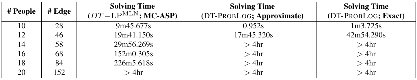
Figure 1: Running Statistics of Algorithm 1 on Marketing Domain

4 $p{\cal BC}+$ with Utility

We extend $p{\cal BC}+$ by introducing the following expression called utility law that assigns a reward to transitions:

$$\hbox{\bf reward}\ v\ {\bf if}\ F\ {\bf after}\ G$$ (20)

where $v$ is a real number representing the reward, $F$ is a formula that contains fluent constants only, and $G$ is a formula that contains fluent constants and action constants only (no pf, no initpf constants). We extend the signature of $Tr(D,m)$ with a set of atoms of the form (16). We turn a utility law of the form (20) into the ${\rm LP}^{\rm{MLN}}$ rule

$$\alpha:{\tt utility}(v,i+1,id)\ \leftarrow\ (i+1:F)\wedge(i:G)$$ (21)

where $id$ is a unique number assigned to the ${\rm LP}^{\rm{MLN}}$ rule and $i\in\{0,\dots,m\!-\!1\}$.

Given a nonnegative integer $m$ denoting the maximum time step, a $p{\cal BC}+$ action description $D$ with utility over multi-valued propositional signature $\sigma$ is defined as a high-level representation of the ${\rm DT}{\mathchar 45\relax}{\rm LP}^{\rm{MLN}}$ program $(Tr(D,m),\sigma^{act}_{m})$.

We extend the definition of a probabilistic transition system as follows.

Definition 7

A probabilistic transition system $T(D)$ represented by a probabilistic action description $D$ is a labeled directed graph such that the vertices are the states of $D$, and the edges are obtained from the transitions of $D$: for every transition $\langle s,e,s^{\prime}\rangle$ of $D$, an edge labeled $e:p,u$ goes from $s$ to $s^{\prime}$, where $p=Pr_{D_{1}}(1\!:\!s^{\prime}\mid 0\!:\!s\wedge 0\!:\!e)$ and $u=E[U_{D_{1}}(0\!:\!s\wedge 0\!:\!e\wedge 1\!:\!s^{\prime})]$. The number $p$ is called the transition probability of $\langle s,e,s^{\prime}\rangle$, denoted by $p(s,e,s^{\prime})$, and the number $u$ is called the transition reward of $\langle s,e,s^{\prime}\rangle$, denoted by $u(s,e,s^{\prime})$.

Example 3

The following action description $D^{simple}$ describes a simple probabilistic action domain with two Boolean fluents $P$, $Q$, and two actions $A$ and $B$. $A$ causes $P$ to be true with probability $0.8$, and if $P$ is true, then $B$ causes $Q$ to be true with probability $0.7$. The agent receives the reward $10$ if $P$ and $Q$ become true for the first time (after that, it remains in the state $\{P,Q\}$ as it is an absorbing state).

$$\begin{array}[]{l}A\ \hbox{\bf causes}\ P\ \hbox{\bf if}\ \hbox{Pf\/}_{1}\\ B\ \hbox{\bf causes}\ Q\ \hbox{\bf if}\ P\wedge\hbox{Pf\/}_{2}\\ \hbox{\bf inertial}\ P,Q\\ \hbox{\bf constraint}\ \neg(Q\wedge\sim\!\!P)\\ \hbox{\bf caused}\ \hbox{Pf\/}_{1}=\{\hbox{\sc true}:0.8,\hbox{\sc false}:0.2\}\\ \hbox{\bf caused}\ \hbox{Pf\/}_{2}=\{\hbox{\sc true}:0.7,\hbox{\sc false}:0.3\}\end{array}$$

$$\begin{array}[]{l}\hbox{\bf reward}\ 10\ \hbox{\bf if}\ P\wedge Q\ \hbox{\bf after}\ \neg(P\wedge Q)\\ \hbox{\bf caused}\ \hbox{InitP\/}=\{\hbox{\sc true}:0.6,\hbox{\sc false}:0.4\}\\ \hbox{\bf initially}\ P=x\ \hbox{\bf if}\ \hbox{InitP\/}=x\\ \hbox{\bf caused}\ \hbox{InitQ\/}=\{\hbox{\sc true}:0.5,\hbox{\sc false}:0.5\}\\ \hbox{\bf initially}\ Q\ \hbox{\bf if}\ \hbox{InitQ\/}\wedge P\\ \hbox{\bf initially}\ \sim\!\!Q\ \hbox{\bf if}\ \sim\!\!P.\end{array}$$

The transition system $T(D^{simple})$ is as follows:

4.1 Policy Optimization

Given a $p{\cal BC}+$ action description $D$, we use ${\bf S}$ to denote the set of states, i.e, the set of interpretations $I^{fl}$ of $\sigma^{fl}$ such that $0\!:\!I^{fl}$ is a residual (probabilistic) stable model of $D_{0}$. We use ${\bf A}$ to denote the set of interpretations $I^{act}$ of $\sigma^{act}$ such that $0\!:\!I^{act}$ is a residual (probabilistic) stable model of $D_{1}$. Since we assume at most one action is executed each time step, each element in ${\bf A}$ makes either only one action or none to be true.

A (non-stationary) policy $\pi$ (in $p{\cal BC}+$) is a function $\pi:{\bf S}\times\{0,\dots,m-1\}\mapsto{\bf A}$ that maps a state and a time step to an action (including doing nothing). By $\langle s_{0},s_{1}\dots,s_{m}\rangle^{t}$ (each $s_{i}\in{\bf S}$) we denote the formula $0\!:\!s_{0}\wedge 1\!:\!s_{1}\wedge\dots\wedge m\!:\!s_{m}$, and by
$\langle s_{0},a_{0},s_{1}\dots,s_{m-1},a_{m-1},s_{m}\rangle^{t}$ (each $s_{i}\in{\bf S}$ and each $a_{i}\in{\bf A}$) the formula

$$0\!:\!s_{0}\wedge 0\!:\!a_{0}\wedge 1\!:\!s_{1}\wedge\dots\wedge m-1\!:\!a_{m-1}\wedge m\!:\!s_{m}.$$

We say a state $s$ is consistent with $D_{init}$ if there exists at least one probabilistic stable model $I$ of $D_{init}$ such that $I\models 0\!:\!s$.

Definition 8

The Policy Optimization problem from the initial state $s_{0}$ is to find a policy $\pi$ that maximizes the expected utility starting from $s_{0}$, i.e., $\pi$ with

$$\underset{\text{$\pi$ is a policy}}{\rm argmax}\ E[U_{Tr(\Pi,m)}(C_{\pi,m}\wedge\langle s_{0}\rangle^{t})]$$

where $C_{\pi,m}$ is the following formula representing policy $\pi$:

$$\underset{s\in{\bf S},\ \pi(s,i)=a,\ i\in\{0,\dots,m-1\}}{\bigwedge}i\!:\!s\rightarrow i\!:\!a\ .$$

We define the total reward of a history $\mathbf{h}=\langle s_{0},a_{0},s_{1},\dots,s_{m}\rangle$ under the action description $D$ as

$$R_{D}(\mathbf{h})=E[U_{Tr(D,m)}(\mathbf{h}^{t})].$$

Although it is defined as an expectation, the following proposition tells us that any stable model $X$ of $Tr(D,m)$ such that $X\models\mathbf{h}$ has the same utility, and consequently, the expected utility of $\mathbf{h}$ is the same as the utility of any single stable model that satisfies the history.

Proposition 2

For any two stable models $X_{1},X_{2}$ of $Tr(D,m)$ that satisfy a history
$\mathbf{h}=\langle s_{0},a_{0},s_{1},a_{1},\dots,a_{m-1},s_{m}\rangle$, we have

$$U_{Tr(D,m)}(X_{1})\ =\ U_{Tr(D,m)}(X_{2})\ =\ E[U_{Tr(D,m)}(\mathbf{h}^{t})].$$

It can be seen that the expected utility of $\pi$ can be computed from the expected utility from all possible state sequences. For any state sequence $\mathbf{s}=\langle s_{0},\dots,s_{m}\rangle$ and any policy $\pi$, we use $\mathbf{h}_{\pi}(\mathbf{s})$ to denote the history obtained by applying $\pi$ on $\mathbf{s}$, i.e.,

$$\mathbf{h}_{\pi}(\mathbf{s})=\langle s_{0},\pi(s_{0},0),s_{1},\dots,\pi(s_{m-1},m-1),s_{m}\rangle.$$

Proposition 3

Given any initial state $s_{0}$ that is consistent with $D_{init}$, for any policy $\pi$, we have

$$\begin{array}[]{l}\small E[U_{Tr(D,m)}(C_{\pi,m}\wedge\langle s_{0}\rangle^{t})]=\\ \underset{\mathbf{s}=\langle s_{1},\dots,s_{m}\rangle:s_{i}\in{\bf S}}{\sum}R_{D}(\mathbf{h}_{\pi}(\mathbf{s})^{t})\times P_{Tr(D,m)}(\mathbf{s}^{t}\wedge C_{\pi,m}).\end{array}$$

Definition 9

For a $p{\cal BC}+$ action description $D$, let $M(D)$ be the MDP $\langle S,A,T,R\rangle$ where (i) the state set $S$ is ${\bf S}$; (ii) the action set $A$ is ${\bf A}$; (iii) transition probability function $T$ is defined as $T(s,a,s^{\prime})=P_{D_{1}}(1:s^{\prime}\mid 0:s\wedge 0:a)$; (iv) reward function $R$ is defined as $R(s,a,s^{\prime})=E[U_{D_{1}}(0:s\wedge 0:a\wedge 1:s^{\prime})]$.

We show that the policy optimization problem for a $p{\cal BC}+$ action description $D$ can be reduced to the policy optimization problem for $M(D)$ for the finite horizon. The following theorem tells us that for any history following a non-stationary policy, its total reward and probability under $D$ defined under the $p{\cal BC}+$ semantics coincide with those under the corresponding MDP $M(D)$.

Theorem 3

Given an initial state $s_{0}\in{\bf S}$ that is consistent with $D_{init}$, for any non-stationary policy $\pi$ and any finite state sequence $\mathbf{s}=\langle s_{0},s_{1},\dots,s_{m-1},s_{m}\rangle$ such that each $s_{i}$ in ${\bf S}\ (i\in\{0,\dots,m\})$, we have

• $R_{D}(\mathbf{h}_{\pi}(\mathbf{s}))=R_{M(D)}(\mathbf{h}_{\pi}(\mathbf{s}))$

• $P_{Tr(D,m)}(\mathbf{s}^{t}\mid\langle s_{0}\rangle^{t}\wedge C_{\pi,m})=P_{M(D)}(\mathbf{h}_{\pi}(\mathbf{s}))$.

It follows that the policy optimization problem for $p{\cal BC}+$ action descriptions coincides with the policy optimization problem for MDP with finite horizon.

Theorem 4

For any nonnegative integer $m$ and an initial state $s_{0}\in{\bf S}$ that is consistent with $D_{init}$, we have

$$\underset{\text{$\pi$ is a non-stationary policy}}{\rm argmax}\ E[U_{Tr(D,m)}(C_{\pi,m}\wedge\langle s_{0}\rangle^{t})]=\underset{\text{$\pi$ is a non-stationary policy}}{\rm argmax}\ \hbox{ER\/}_{M(D)}(\pi,s_{0}).$$

Theorem 4 justifies using an implementation of ${\rm DT}{\mathchar 45\relax}{\rm LP}^{\rm{MLN}}$ to compute optimal policies of MDP $M(D)$ as well as using an MDP solver to compute optimal policies of the $p{\cal BC}+$ descriptions. Furthermore, the theorems above allow us to check the properties of MDP $M(D)$ by using formal properties of ${\rm LP}^{\rm{MLN}}$, such as whether a certain state is reachable in a given number of steps.

5 $p{\cal BC}+$ as a High-Level Representation Language of MDP

An action description consists of causal laws in a human-readable form describing the action domain in a compact and high-level way, whereas it is non-trivial to describe an MDP instance directly from the domain description in English. The result in the previous section shows how to construct an MDP instance $M(D)$ for a $p{\cal BC}+$ action description $D$ so that the solution to the policy optimization problem of $D$ coincides with that of MDP $M(D)$. In that sense, $p{\cal BC}+$ can be viewed as a high-level representation language for MDP.

Since ${\rm LP}^{\rm{MLN}}$ programs are weighted rules under the stable model semantics, and the semantics of $p{\cal BC}+$ is defined in terms of ${\rm LP}^{\rm{MLN}}$, $p{\cal BC}+$ inherits the nonmonotonicity of the stable model semantics to be able to compactly represent recursive definitions or transitive closure [Erdem et al. (2016)]. The static laws in $p{\cal BC}+$ prune out invalid states to ensure that only meaningful value combinations of fluents will be given to MDP as states, thus reducing the size of state space at the MDP level. To demonstrate this, we show how Example 1 (Robot and Blocks) can be represented in $p{\cal BC}+$ as follows.

First we define the signature of the action description: $x,x_{1},x_{2}$ are schematic variables that range over ${\tt B1}$, ${\tt B2}$, ${\tt B3}$; $r,r_{1},r_{2}$ range over ${\tt R1}$, ${\tt R2}$. $\hbox{TopClear\/}(x)$, $\hbox{Above\/}(x_{1},x_{2})$, and GoalNotAchieved are Boolean statically determined fluent constants; $\hbox{In\/}(x)$ is a regular fluent constant with domain $\{{\tt R1},{\tt R2}\}$, and $\hbox{OnTopOf\/}(x_{1},x_{2})$ is a Boolean regular fluent constant. $\hbox{MoveTo\/}(x,r)$ and $\hbox{StackOn\/}(x_{1},x_{2})$ are action constants and Pf_Move is a Boolean pf constant. In this example, we make the goal state absorbing, i.e., when all the blocks are already in R2, then all actions have no effect.

Moving block $x$ to room $r$ causes $x$ to be in $r$ with probability $p$:

$$\begin{array}[]{l}\hbox{MoveTo\/}(x,r)\ \hbox{\bf causes}\ \hbox{In\/}(x)=r\ \hbox{\bf if}\ \hbox{Pf\_Move\/}\wedge\hbox{GoalNotAchieved\/}\\ \hbox{\bf caused}\ \hbox{Pf\_Move\/}=\{\hbox{\sc true}:p,\hbox{\sc false}:1-p\}.\end{array}$$

If a block $x_{1}$ is on top of another block $x_{2}$, then successfully moving $x_{1}$ to a different room $r_{2}$ causes $x_{1}$ to be no longer on top of $x_{2}$:

$$\begin{array}[]{l}\hbox{MoveTo\/}(x_{1},r_{2})\ \hbox{\bf causes}\ \sim\!\hbox{OnTopOf\/}(x_{1},x_{2})\\ \hskip 42.67912pt\hbox{\bf if}\ \hbox{Pf\_Move\/}\wedge\hbox{In\/}(x_{1})=r_{1}\wedge\hbox{OnTopOf\/}(x_{1},x_{2})\wedge\hbox{GoalNotAchieved\/}\ \ \ \ (r_{1}\neq r_{2}).\end{array}$$

Stacking a block $x_{1}$ on another block $x_{2}$ causes $x_{1}$ to be on top of $x_{2}$, if the top of $x_{2}$ is clear, and $x_{1}$ and $x_{2}$ are at the same location:

$$\hbox{StackOn\/}(x_{1},x_{2})\ \hbox{\bf causes}\ \hbox{OnTopOf\/}(x_{1},x_{2})$$

$$\hskip 28.45274pt\hbox{\bf if}\ \hbox{TopClear\/}(x_{2})\wedge\hbox{At\/}(x_{1})=r\wedge\hbox{At\/}(x_{2})=r\wedge\hbox{GoalNotAchieved\/}\hskip 28.45274pt(x_{1}\neq x_{2}).$$

Stacking a block $x_{1}$ on another block $x_{2}$ causes $x_{1}$ to be no longer on top of the block $x$ where $x_{1}$ was originally on top of:

$$\hbox{StackOn\/}(x_{1},x_{2})\ \hbox{\bf causes}\ \sim\!\hbox{OnTopOf\/}(x_{1},x)\ \hbox{\bf if}\ \hbox{TopClear\/}(x_{2})\wedge\hbox{At\/}(x_{1})=r\wedge\hbox{At\/}(x_{2})=r\wedge$$

$$\ \ \ \ \ \ \ \ \ \ \ \ \hbox{OnTopOf\/}(x_{1},x)\wedge\hbox{GoalNotAchieved\/}\ \hskip 99.58464pt(x_{2}\neq x,x_{1}\neq x_{2}).$$

Two different blocks cannot be on top of the same block, and a block cannot be on top of two different blocks:

$$\begin{array}[]{l}\hbox{\bf constraint}\ \neg(\hbox{OnTopOf\/}(x_{1},x)\wedge\hbox{OnTopOf\/}(x_{2},x))\ \hskip 71.13188pt(x_{1}\neq x_{2})\\ \hbox{\bf constraint}\ \neg(\hbox{OnTopOf\/}(x,x_{1})\wedge\hbox{OnTopOf\/}(x,x_{2}))\ \hskip 71.13188pt(x_{1}\neq x_{2}).\end{array}$$

By default, the top of a block $x$ is clear. It is not clear if there is another block $x_{1}$ that is on top of it:

$$\begin{array}[]{l}\hbox{\bf default}\ \hbox{TopClear\/}(x)\\ \hbox{\bf caused}\ \sim\!\hbox{TopClear\/}(x)\ \hbox{\bf if}\ \hbox{OnTopOf\/}(x_{1},x).\end{array}$$

The relation $Above$ between two blocks is the transitive closure of the relation OnTopOf: A block $x_{1}$ is above another block $x_{2}$ if $x_{1}$ is on top of $x_{2}$, or there is another block $x$ such that $x_{1}$ is above $x$ and $x$ is above $x_{2}$:

$$\begin{array}[]{l}\hbox{\bf caused}\ \hbox{Above\/}(x_{1},x_{2})\ \hbox{\bf if}\ \hbox{OnTopOf\/}(x_{1},x_{2})\\ \hbox{\bf caused}\ \hbox{Above\/}(x_{1},x_{2})\ \hbox{\bf if}\ \hbox{Above\/}(x_{1},x)\wedge\hbox{Above\/}(x,x_{2}).\end{array}$$

One block cannot be above itself; two blocks cannot be above each other:

$$\begin{array}[]{l}\hbox{\bf caused}\ \bot\ \hbox{\bf if}\ \hbox{Above\/}(x_{1},x_{2})\wedge\hbox{Above\/}(x_{2},x_{1}).\end{array}$$

If a block $x_{1}$ is above another block $x_{2}$, then $x_{1}$ has the same location as $x_{2}$:

$$\begin{array}[]{l}\hbox{\bf caused}\ \hbox{At\/}(x_{1})=r\ \hbox{\bf if}\ \hbox{Above\/}(x_{1},x_{2})\wedge\hbox{At\/}(x_{2})=r.\end{array}$$ (22)

Each moving action has a cost of $1$:

$$\begin{array}[]{l}\hbox{\bf reward}\ -1\ \hbox{\bf if}\ \top\ \hbox{\bf after}\ \hbox{MoveTo\/}(x,r).\end{array}$$

Achieving the goal when the goal is not previously achieved yields a reward of $10$:

$$\begin{array}[]{l}\hbox{\bf reward}\ 10\ \hbox{\bf if}\ \sim\!\hbox{GoalNotAchieved\/}\ \hbox{\bf after}\ \hbox{GoalNotAchieved\/}.\end{array}$$

The goal is not achieved if there exists a block $x$ that is not at ${\tt R2}$. It is achieved otherwise:

$$\begin{array}[]{l}\hbox{\bf caused}\ \hbox{GoalNotAchieved\/}\ \hbox{\bf if}\ \hbox{At\/}(x)=r\ \ (r\neq{\tt R2})\\ \hbox{\bf default}\ \sim\!\hbox{GoalNotAchieved\/}.\end{array}$$

$\hbox{At\/}(x)$ and $\hbox{OnTopOf\/}(x_{1},x_{2})$ are inertial:

$$\begin{array}[]{l}\hbox{\bf inertial}\ \hbox{At\/}(x),\hbox{OnTopOf\/}(x_{1},x_{2}).\end{array}$$

Finally, we add   $a_{1}\wedge a_{2}\ \hbox{\bf causes}\ \bot$   for each distinct pair of ground action constants $a_{1}$ and $a_{2}$, to ensure that at most one action can occur each time step.

It can be seen that stacking all blocks together and moving them at once would be the best strategy to move them to ${\tt R2}$.

In the robot and blocks example, many value combinations of fluents do not lead to a valid state, such as

$$\{\hbox{OnTopOf\/}({\tt B1},{\tt B2}),\hbox{OnTopOf\/}({\tt B2},{\tt B1}),...\},$$

where the two blocks ${\tt B1}$ and ${\tt B2}$ are on top of each other. Moreover, the fluents $\hbox{TopClear\/}(x)$ and $\hbox{Above\/}(x_{1},x_{2})$ are completely dependent on the value of the other fluents. There would be $2^{3+3\times 3+3+3\times 3}=2^{24}$ states if we define a state as any value combination of fluents. On the other hand, the static laws in the above action description reduce the number of states to only $(13+9)\times 2=44$. To see this, consider all possible configuration with $3$ blocks and $2$ locations. As illustrated in Figure 2, there are $13$ possible configurations with $3$ blocks on the same side, and $9$ possible configurations with one block one one side and two on the other side. Each configureration can be mirrored to yield another configuration, so we have $(13+9)\times 2=44$ in total. This is aligned with the number of MDP states obtained from the $p{\cal BC}+$ action description according to Definition 9.

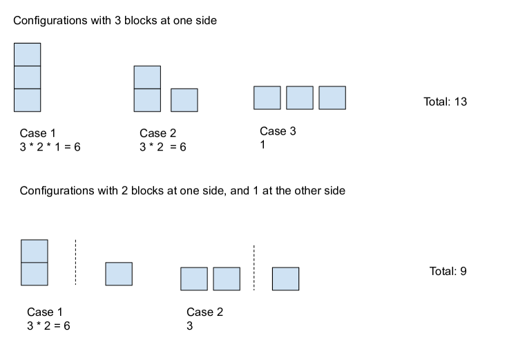
Figure 2: Possible Configurations with $3$ blocks and $2$ locations

Furthermore, in this example, $\hbox{Above\/}(x,y)$ needs to be defined as a transitive closure of $\hbox{OnTopOf\/}(x,y)$, so that the effects of $\hbox{StackOn\/}(x_{1},x_{2})$ can be defined in terms of the (inferred) spatial relation of blocks. Also, the static law (22) defines an indirect effect of $\hbox{MoveTo\/}(x,r)$.

6 System pbcplus2mdp

We implement system pbcplus2mdp, which takes the ${\rm LP}^{\rm{MLN}}$ translation of an action description $D$ and time horizon $m$ as input, and finds the optimal policy by constructing the corresponding MDP $M(D)$ and utilizing MDP policy optimization algorithms as black box. We use mdptoolbox as our underlying MDP solver. The current system uses ${\rm LP}^{\rm{MLN}}$ 1.0 ( http://reasoning.eas.asu.edu/lpmln/index.html) for exact inference to find states, actions, transition probabilities and transition rewards. The system is publically available at https://github.com/ywang485/pbcplus2mdp [Wang (2020)], along with several examples.

We measure the scalability of our system pbcplus2mdp on the robot and blocks example. Figure 3 shows the running statistics of finding the optimal policy for different number of blocks. For all of the running instances, maximum time horizon is set to be $10$, as in all of the instances, the smallest number of steps in a shortest possible action sequence achieving the goal is less than $10$. The discount factor is set to be $0.9$. The experiments are performed on a machine with 4 Intel(R) Core(TM) i5-2400 CPU with OS Ubuntu 14.04.5 LTS and 8 GB memory.

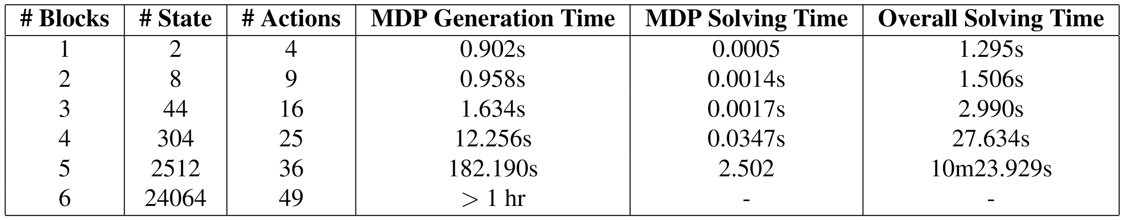
Figure 3: Running Statistics of pbcplus2mdp system

As can be seen from the table, the running time increases exponentially as the number of blocks increases. This is not surprising since the size of the search space increases exponentially as the number of blocks increases. The bottleneck is the ${\rm LP}^{\rm{MLN}}$ inference system, as it needs to enumerate every stable model to generate the set of states, the set of actions, transition probabilities and rewards. Time spent on MDP planning is negligible.

Since the bottleneck is the size of the domain, one potential direction of improving the scalability would be to represent the action description at first-order level, and then utilize planning algorithms for first-order MDPs, such as [Boutilier et al. (2001), Yoon et al. (2002), Wang et al. (2008), Sanner and Boutilier (2009)], to compute domain-independent policies. This method requires a solver for first-order ${\rm LP}^{\rm{MLN}}$. We leave this for future work.

System pbcplus2mdp supports planning with infinite horizon. However, it should be noted that the semantics of an action description with infinite time horizon in terms of $DT-{\rm LP}^{\rm{MLN}}$ is not yet well established. In this case, the action description is only viewed as a high-level representation of an MDP.

7 Related Work

There have been quite a few studies and attempts in defining factored representations of (PO)MDP, with feature-based state descriptions and more compact, human-readable action definitions. PPDDL [Younes and Littman (2004)] extends PDDL with constructs for describing probabilistic effects of actions and reward from state transitions. One limitation of PPDDL is the lack of static causal laws, which prohibits PPDDL from expressing recursive definitions or transitive closure. This may yield a large state space to explore as discussed in Section 5. RDDL (Relational Dynamic Influence Diagram Language) [Sanner (2010)] improves the expressivity of PPDDL in modeling stochastic planning domains by allowing concurrent actions, continuous values of fluents, state constraints, etc. The semantics is defined in terms of lifted dynamic Bayes network extended with influence graph. A lifted planner can utilize the first-order representation and potentially achieve better performance. Still, indirect effects are hard to be represented in RDDL. Compared to PPDDL and RDDL, the advantages of $p\cal{BC}+$ are in its simplicity and expressivity originating from the stable model semantics, which allows for elegant representation of recursive definitions, defeasible behaviors, and indirect effects.

[Poole (2013)] combines the Situation Calculus [McCarthy (1963)] and the Independent Choice Logic (ICL) [Poole (2008)] for probabilistic planning. The situation calculus is used to specify effects of actions, and ICL is used to model randomness in an action domain. The notion of choice alternatives in ICL is similar to pf constant in $p{\cal BC}+$, and an atomic choice resembles a value assignment to a pf constant. While $p{\cal BC}+$ allows uncertainty to be from both probabilities and logic, [Poole (2013)] has the restriction that all the uncertainty comes from probabilities, i.e., the logic program is required to have a unique model once all the independent choices are fixed. Another difference is that [Poole (2013)] considers only acyclic logic program (which is not a restriction in $p{\cal BC}+$), and it is thus not straightforward to represent transitive closure such as “a block being moved causes the block on top of it also being moved”, as in Example 1. It is worth noting that [Poole (2013)] allows a more compact and flexible representation of policies, where conditional expressions can be used to summarize the action to take for a set of states where a certain sensor value is observed.

[Zhang and Stone (2015)] adopt ASP and P-Log [Baral et al. (2009)] which respectively produces a refined set of states and a refined probability distribution over states that are then fed to POMDP solvers for low-level planning. The refined sets of states and probability distribution over states take into account commonsense knowledge about the domain, and thus improve the quality of a plan and reduce computation needed at the POMDP level. [Yang et al. (2018)] adopts the (deterministic) action description language $\cal{BC}$ for high-level representations of the action domain, which defines high-level actions that can be treated as deterministic. Each action in the generated high-level plan is then mapped into more detailed low-level policies, which takes stochastic effects of low-level actions into account. Similarly, [Sridharan et al. (2015)] introduce a framework with planning in a coarse-resolution transition model and a fine-resolution transition model. Action language ${\cal AL}_{d}$ is used for defining the two levels of transition models. The fine-resolution transition model is further turned into a POMDP for detailed planning with stochastic effects of actions and transition rewards. While a $p\cal{BC}+$ action description can fully capture all aspects of (PO)MDP including transition probabilities and rewards, the ${\cal AL}_{d}$ action description only provides states, actions and transitions with no quantitative information. [Leonetti et al. (2016)], on the other hand, use symbolic reasoners such as ASP to reduce the search space for reinforcement learning based planning methods by generating partial policies from planning results generated by the symbolic reasoner. The exploration of the low-level RL module is constrained by actions that satisfy the partial policy.

Another related work is [Ferreira et al. (2017)], which combines ASP and reinforcement learning by using action language $\cal{BC}+$ as a meta-level description of MDP. The $\cal{BC}+$ action descriptions define non-stationary MDPs in the sense that the states and actions can change with new situations occurring in the environment. The algorithm ASP(RL) proposed in this work iteratively calls an ASP solver to obtain states and actions for the RL methods to learn transition probabilities and rewards, and updates the $\cal{BC}+$ action description with changes in the environment found by the RL methods, in this way finding optimal policy for a non-stationary MDP with the search space reduced by ASP. The work is similar to ours in that ASP-based high-level logical description is used to generate states and actions for MDP, but the difference is that we use an extension of ${\cal BC}$+ that expresses transition probabilities and rewards.

8 Conclusion

In this work, we bridge the gap between action language $p{\cal BC}+$ and Markov Decision Process by extending $p{\cal BC}+$ with the notion of utility, which allows $p{\cal BC}+$ to serve as an elaboration tolerant representation of MDP, as well as leveraging an MDP solver to compute a $p{\cal BC}+$ action description. Our main contributions are as follows.

• We extended ${\rm LP}^{\rm{MLN}}$ with the notion of utility, resulting in ${\rm DT}{\mathchar 45\relax}{\rm LP}^{\rm{MLN}}$; we developed an approximate algorithm for maximizing expected utility in ${\rm DT}{\mathchar 45\relax}{\rm LP}^{\rm{MLN}}$;

• Based on ${\rm DT}{\mathchar 45\relax}{\rm LP}^{\rm{MLN}}$, we extended $p{\cal BC}+$ with the notion of utility;

• We showed that the semantics of $p{\cal BC}+$ can be alternatively defined in terms of Markov Decision Process;

• We demonstrated how $p{\cal BC}+$ can serve as an elaboration tolerant representation of MDP;

• We developed a prototype system pbcplus2mdp, for finding optimal policies of $p{\cal BC}+$ action descriptions using an MDP solver.

Formally relating action languages and MDP opens up interesting research to explore. Dynamic programming methods in MDP can be utilized to compute action languages. In turn, action languages may serve as a formal verification tool for MDP as well as a high-level representation language for MDP that describes an MDP instance in a succinct and elaboration tolerant way. As many reinforcement learning tasks use MDP as a modeling language, the work may be related to incorporating symbolic knowledge to reinforcement learning as evidenced by [Zhang and Stone (2015), Yang et al. (2018), Leonetti et al. (2016)].

${\rm DT}{\mathchar 45\relax}{\rm LP}^{\rm{MLN}}$ may deserve attention on its own for static domains. We expect that this extension of ${\rm LP}^{\rm{MLN}}$ system that can handle utility can be a useful tool for verifying properties for MDP.

The theoretical results in this paper limit attention to MDP in the finite horizon case. When the maximum step $m$ is sufficiently large, we may view it as an approximation of the infinite horizon case, in which case, we allow discount factor $\gamma$ by replacing $v$ in (21) with $\gamma^{i+1}v$. While it appears intuitive to extend the theoretical results in this paper to the infinite case, it requires extending the definition of ${\rm LP}^{\rm{MLN}}$ to allow infinitely many rules, which we leave for future work.

Acknowledgements: We are grateful to the anonymous referees for their useful comments and to Siddharth Srivastava, Zhun Yang, and Yu Zhang for helpful discussions. This work was partially supported by the National Science Foundation under Grant IIS-1815337.

Appendix A Proofs

Proofs of Theorem 1, 2 and Corollary 1 can be found in the supplimentary material of [Lee and Wang (2018)].

A.1 Propositions and Lemmas

We write $\langle a_{0},a_{1}\dots,a_{m-1}\rangle^{t}$ (each $a_{i}\in{\bf A}$) to denote the formula $0\!:\!a_{0}\wedge 1\!:\!a_{1}\dots\wedge m-1\!:\!a_{m-1}$. The following lemma tells us that any action sequence has the same probability under $Tr(D,m)$.

For any multi-valued probabilistic program $\Pi$, let $pf_{1},\dots,pf_{m}$ be the probabilistic constants in $\Pi$, and $v_{i,1},\dots,v_{i,k_{i}}$, each associated with probability $p_{i,1},\dots,p_{i,k_{i}}$ resp. be the values of $pf_{i}$ ($i\in\{1,\dots,m\}$). We use $TC_{\Pi}$ be the set of all assignments to probabilistic constants in $\Pi$.

Lemma 1

For any $p\cal{BC}+$ action description $D$ and any action sequence $\mathbf{a}=\langle a_{0},a_{1},\dots,a_{m-1}\rangle$, we have

$$P_{Tr(D,m)}(\mathbf{a}^{t})=\frac{1}{(|\sigma^{act}|+1)^{m}}.$$

Proof A.1.

$$P_{Tr(D,m)}(\mathbf{a}^{t})$$

$$=\ \underset{\begin{subarray}{c}I\vDash\mathbf{a}^{t}\\ \text{$I$ is a stable models of $Tr(D,m)$}\end{subarray}}{\sum}P_{Tr(D,m)}(I)$$

$$=\ Tr(D,m) (|\sigma^{act}|+1)^{m}$$ (In every total choice leads to stable models. By Proposition 2 in [Lee and Wang (2018)], )

$$\underset{\begin{subarray}{c}I\vDash\mathbf{a}^{t}\\ \text{$I$ is a stable models of $Tr(D,m)$}\end{subarray}}{\sum}\frac{W_{Tr(D,m)}(I)}{(|\sigma^{act}|+1)^{m}}$$

$$=\ \frac{\underset{tc\in TC_{Tr(D,m)}}{\sum}\underset{c=v\in tc}{\prod}M_{\Pi}(c=v)}{(|\sigma^{act}|+1)^{m}}$$

$$=\$$ (Derivations same as in the proof of Proposition 2 in [Lee and Wang (2018)])

$$\frac{1}{(|\sigma^{act}|+1)^{m}}$$

The following lemma states that given any action sequence, the probabilities of all possible state sequences sum up to $1$.

Lemma A.2.

For any $p\cal{BC}+$ action description $D$ and any action sequence $\mathbf{a}=\langle a_{0},a_{1},\dots,a_{m-1}\rangle$, we have

$$\underset{s_{0},\dots,s_{m}:s_{i}\in{\bf S}}{\sum}P_{Tr(D,m)}(\langle s_{0},\dots,s_{m}\rangle^{t}\mid\mathbf{a}^{t})=1.$$

Proof A.3.

$$\underset{s_{0},\dots,s_{m}:s_{i}\in{\bf S}}{\sum}P_{Tr(D,m)}(\langle s_{0},\dots,s_{m}\rangle^{t}\mid\mathbf{a}^{t})$$

$$=\$$ (By Corollary 1 in [Lee and Wang (2018)])

$$\underset{s_{0},\dots,s_{m}:s_{i}\in{\bf S}}{\sum}\underset{i\in\{0,\dots,m-1\}}{\prod}p(s_{i},a_{i},s_{i+1})$$

$$=\ \underset{s_{0}\in{\bf S}}{\sum}(p(s_{0})\cdot\underset{s_{1},\dots,s_{m}:s_{i}\in{\bf S}}{\sum}\underset{i\in\{1,\dots,m-1\}}{\prod}p(s_{i},a_{i},s_{i+1}))$$

$$=\ \underset{s_{0}\in{\bf S}}{\sum}(p(s_{0})\cdot\underset{s_{1}\in{\bf S}}{\sum}(p(s_{0},a_{0},s_{1})\cdot\underset{s_{2},\dots,s_{m}:s_{i}\in{\bf S}}{\sum}\underset{i\in\{2,\dots,m-1\}}{\prod}p(s_{i},a_{i},s_{i+1})))$$

$$=\ \underset{s_{0}\in{\bf S}}{\sum}(p(s_{0})\cdot\underset{s_{1}\in{\bf S}}{\sum}(p(s_{0},a_{0},s_{1})\cdot\dots\cdot\underset{s_{m}\in{\bf S}}{\sum}p(s_{m-1},a_{i},s_{m})\dots))$$

$$=\ 1.$$

The following proposition tells us that the probability of any state sequence conditioned on the constraint representation of a policy $\pi$ coincide with the probability of the state sequence conditioned on the action sequence specified by $\pi$ w.r.t. the state sequence.

Proposition 5.

For any $p\cal{BC}+$ action description $D$, state sequence $\mathbf{s}=\langle s_{0},s_{1},\dots,s_{m}\rangle$, and a non-stationary policy $\pi$, we have

$$P_{Tr(D,m)}(\mathbf{s}^{t}\mid C_{\pi,m})=$$

$$P_{Tr(D,m)}(\mathbf{s}^{t}\mid\langle\pi(s_{0},0),\pi(s_{1},1),\dots,\pi(s_{m-1},m-1)\rangle^{t})$$

Proof A.4.

$$P_{Tr(D,m)}(\mathbf{s}^{t}\mid C_{\pi,m})$$

$$=\ \frac{P_{Tr(D,m)}(\langle s_{0},\dots,s_{m}\rangle^{t}\wedge C_{\pi,m})}{P_{Tr(D,m)}(C_{\pi,m})}$$

$$=\ \frac{P_{Tr(D,m)}(\langle s_{0},\pi(s_{0},0)\dots,\pi(s_{m-1},m-1),s_{m}\rangle^{t}}{P_{Tr(D,m)}(C_{\pi,m})}$$

$$=\ \frac{P_{Tr(D,m)}(\langle\pi(s_{0},0)\dots,\pi(s_{m-1},m-1),s_{m}\rangle^{t}\mid 0\!:\!s_{0})\cdot P_{Tr(D,m)}(0\!:\!s_{0})}{\underset{s^{\prime}_{0},\dots,s^{\prime}_{m}:s^{\prime}_{i}\in{\bf S}}{\sum}P_{Tr(D,m)}(\langle s^{\prime}_{0},\pi(s^{\prime}_{0},0)\dots,\pi(s^{\prime}_{m-1},m-1),s^{\prime}_{m}\rangle^{t})}.$$

We use $k(s_{0},\dots,s_{m})$ as an abbreviation of

$$P_{Tr(D,m)}(\langle\pi(s_{0},0),\dots,\pi(s_{m-1},m-1)\rangle^{t}).$$

We have

$$P_{Tr(D,m)}(\mathbf{s}^{t}\mid C_{\pi,m})$$

$$=\ \frac{P_{Tr(D,m)}(\langle s_{1},\dots,s_{m}\rangle^{t}\mid\langle s_{0},\pi(s_{0},0),\dots,\pi(s_{m-1},m-1)\rangle^{t})\cdot P_{Tr(D,m)}(0\!:\!s_{0})\cdot k(s_{0},\dots,s_{m})}{\underset{s^{\prime}_{0},\dots,s^{\prime}_{m}:s^{\prime}_{i}\in{\bf S}}{\sum}P_{Tr(D,m)}(\langle s^{\prime}_{1},\dots,s^{\prime}_{m}\rangle^{t}\mid\langle s^{\prime}_{0},\pi(s^{\prime}_{0},0),\dots,\pi(s^{\prime}_{m-1},m-1)\rangle^{t})\cdot P_{Tr(D,m)}(0\!:\!s^{\prime}_{0})\cdot k(s^{\prime}_{0},\dots,s^{\prime}_{m})}$$

$$=\ s_{0},\dots,s_{m}(s_{i}\in{\bf S}) k(s_{0},\dots,s_{m})=\frac{1}{(\sigma^{act}|+1)^{m}}$$ (By Lemma 1, for any , we have )

$$\frac{P_{Tr(D,m)}(\langle s_{1},\dots,s_{m}\rangle^{t}\mid\langle s_{0},\pi(s_{0},0),\dots,\pi(s_{m-1},m-1)\rangle^{t})\cdot P_{Tr(D,m)}(0:s_{0})\cdot\frac{1}{(|\sigma^{act}|+1)^{m}}}{\underset{s^{\prime}_{0},\dots,s^{\prime}_{m}:s^{\prime}_{i}\in{\bf S}}{\sum}P_{Tr(D,m)}(\langle s^{\prime}_{1},\dots,s^{\prime}_{m}\rangle^{t}\mid\langle s^{\prime}_{0},\pi(s^{\prime}_{0},0),\dots,\pi(s^{\prime}_{m-1},m-1)\rangle^{t})\cdot P_{Tr(D,m)}(0\!:\!s^{\prime}_{0})\cdot\frac{1}{(|\sigma^{act}|+1)^{m}}}$$

$$=\ \frac{P_{Tr(D,m)}(\langle s_{1},\dots,s_{m}\rangle^{t}\mid\langle s_{0},\pi(s_{0},0),\dots,\pi(s_{m-1},m-1)\rangle^{t})\cdot P_{Tr(D,m)}(0:s_{0})}{\underset{s^{\prime}_{0},\dots,s^{\prime}_{m}:s^{\prime}_{i}\in{\bf S}}{\sum}P_{Tr(D,m)}(\langle s^{\prime}_{1},\dots,s^{\prime}_{m}\rangle^{t}\mid\langle s^{\prime}_{0},\pi(s^{\prime}_{0},0),\dots,\pi(s^{\prime}_{m-1},m-1)\rangle^{t})\cdot P_{Tr(D,m)}(0\!:\!s^{\prime}_{0})}$$

$$=\ 1$$ (By Lemma A.2, the denominator equals )

$$P_{Tr(D,m)}(\langle s_{1},\dots,s_{m}\rangle^{t}\mid\langle s_{0},\pi(s_{0},0),\dots,\pi(s_{m-1},m-1)\rangle^{t})\cdot P_{Tr(D,m)}(0:s_{0})$$

$$=\ P_{Tr(D,m)}(\langle s_{0},s_{1},\dots,s_{m}\rangle^{t}\mid\langle\pi(s_{0},0),\dots,\pi(s_{m}-1,m-1)\rangle^{t})$$

A.2 Proofs of Proposition 2, Proposition 3, Theorem 3 and Theorem 4

The following proposition tells us that, for any states and actions sequence, any stable model of $Tr(D,m)$ that satisfies the sequence has the same utility. Consequently, the expected utility of the sequence can be computed by looking at any single stable model that satisfies the sequence.

Proposition 2   For any two stable models $X_{1},X_{2}$ of $Tr(D,m)$ that satisfy a history
$\mathbf{h}=\langle s_{0},a_{0},s_{1},a_{1},\dots,a_{m-1},s_{m}\rangle$, we have

$$U_{Tr(D,m)}(X_{1})\ =\ U_{Tr(D,m)}(X_{2})\ =\ E[U_{Tr(D,m)}(\mathbf{h}^{t})].$$

Proof A.5.

Since both $X_{1}$ and $X_{2}$ both satisfy $\mathbf{h}^{t}$, $X_{1}$ and $X_{2}$ agree on truth assignment on $\sigma^{act}_{m}\cup\sigma^{fl}_{m}$. Notice that atom of the form ${\tt utility}(v,{\bf t})$ in $Tr(D,m)$ occurs only of the form (21), and only atom in $\sigma^{act}_{m}\cup\sigma^{fl}_{m}$ occurs in the body of rules of the form (21).

• Suppose an atom ${\tt utility}(v,{\bf t})$ is in $X_{1}$. Then the body $B$ of at least one rule of the form (21) with ${\tt utility}(v,{\bf t})$ in its head in $Tr(D,m)$ is satisfied by $X_{1}$. $B$ must be satisfied by $X_{2}$ as well, and thus ${\tt utility}(v,{\bf t})$ is in $X_{2}$ as well.

• Suppose an atom ${\tt utility}(v,{\bf t})$, is not in $X_{1}$. Then, assume, to the contrary, that ${\tt utility}(v,{\bf t})$ is in $X_{2}$, then by the same reasoning process above in the first bullet, ${\tt utility}(v,{\bf t})$ should be in $X_{1}$ as well, which is a contradiction. So ${\tt utility}(v,{\bf t})$ is also not in $X_{2}$.

So $X_{1}$ and $X_{2}$ agree on truth assignment on all atoms of the form ${\tt utility}(v,{\bf t})$, and consequently we have $U_{Tr(D,m)}(X_{1})=U_{Tr(D,m)}(X_{2})$, as well as

$$E[U_{Tr(D,m)}(\mathbf{h}^{t})]$$

$$=\ \underset{I\vDash\mathbf{h}^{t}}{\sum}P_{Tr(D,m)}(I\mid\mathbf{h}^{t})\cdot U_{Tr(D,m)}(I)$$

$$=\ U_{Tr(D,m)}(X_{1})\cdot\underset{I\vDash\mathbf{h}^{t}}{\sum}P_{Tr(D,m)}(I\mid\mathbf{h}^{t})$$

$$=\ 1$$ (The second term equals )

$$U_{Tr(D,m)}(X_{1}).$$

The following proposition tells us that the expected utility of an action and state sequence can be computed by summing up the expected utility from each transition.

Proposition 6.

For any $p\cal{BC}+$ action description $D$ and a history $\mathbf{h}=\langle s_{0},a_{0},s_{1},\dots,a_{m-1},s_{m}\rangle$, such that there exists at least one stable model of $Tr(D,m)$ that satisfies $\mathbf{h}$, we have

$$E[U_{Tr(D,m)}(\mathbf{h}^{t})]=\underset{i\in\{0,\dots,m-1\}}{\sum}u(s_{i},a_{i},s_{i+1}).$$

Proof A.6.

Let $X$ be any stable model of $Tr(D,m)$ that satisfies $\mathbf{h}^{t}$. By Proposition 2, we have

$$E[U_{Tr(D,m)}(\mathbf{h}^{t})]$$

$$=\ U_{Tr(D,m)}(X)$$

$$=\ \underset{i\in\{0,\dots,m-1\}}{\sum}(\underset{\begin{subarray}{c}utility(v,i,{\bf x})\leftarrow(i+1:F)\wedge(i:G)\in Tr(D,m)\\ \text{$X$ satisfies $(i+1:F)\wedge(i:G)$}\end{subarray}}{\sum}v)$$

$$=\ \underset{i\in\{0,\dots,m-1\}}{\sum}(\underset{\begin{subarray}{c}utility(v,0,{\bf x})\leftarrow(1:F)\wedge(0:G)\in Tr(D,m)\\ \text{$0\!:\!X^{i}$ satisfies $(1:F)\wedge(0:G)$}\end{subarray}}{\sum}v)$$

$$=\ \underset{i\in\{0,\dots,m-1\}}{\sum}U_{Tr(D,1)}(0\!:\!X^{i})$$

$$=\$$ ( By Proposition 2)

$$\underset{i\in\{0,\dots,m-1\}}{\sum}E[U_{Tr(D,1)}(0:s_{i},0:a_{i},1:s_{i+1})]$$

$$=\ \underset{i\in\{0,\dots,m-1\}}{\sum}u(s_{i},a_{i},s_{i+1}).$$

Proposition 3   Given any initial state $s_{0}$ that is consistent with $D_{init}$, for any policy $\pi$, we have

$$\begin{array}[]{l}\small E[U_{Tr(D,m)}(C_{\pi,m}\wedge\langle s_{0}\rangle^{t})]=\\ \underset{\mathbf{s}=\langle s_{1},\dots,s_{m}\rangle:s_{i}\in{\bf S}}{\sum}R_{D}(\mathbf{h}_{\pi}(\mathbf{s})^{t})\times P_{Tr(D,m)}(\mathbf{s}^{t}\wedge C_{\pi,m}).\end{array}$$

Proof A.7.

We have

$$E[U_{Tr(D,m)}(C_{\pi,m}\wedge\langle s_{0}\rangle^{t})]$$

$$=\ \underset{I\vDash 0:s_{0}\wedge C_{\pi,m}}{\sum}P_{Tr(D,m)}(I\mid 0\!:\!s_{0}\wedge C_{\pi,m})\cdot U_{Tr(D,m)}(I)$$

$$=\ \underset{\begin{subarray}{c}I\vDash 0:s_{0}\wedge C_{\pi,m}\\ \text{$I$ is a stable model of $Tr(D,m)$}\end{subarray}}{\sum}P_{Tr(D,m)}(I\mid 0\!:\!s_{0}\wedge C_{\pi,m})\cdot U_{Tr(D,m)}(I)$$

$$=\ I \sigma^{fl}_{m}$$ (We partition stable models according to their truth assignment on )

$$\underset{\mathbf{s}=\langle s_{1},\dots,s_{m}\rangle:s_{i}\in{\bf S}\ \ }{\sum}\underset{\begin{subarray}{c}I\vDash\mathbf{s}^{t}\wedge C_{\pi,m}\\ \text{$I$ is a stable model of $Tr(D,m)$}\end{subarray}}{\sum}P_{Tr(D,m)}(I\mid 0\!:\!s_{0}\wedge C_{\pi,m})\cdot U_{Tr(D,m)}(I)$$

$$=\ I\vDash\mathbf{s}^{t}\wedge C_{\pi,m} I\vDash\mathbf{h}_{\pi}(\mathbf{s})^{t}$$ (Since implies , by Proposition 2 we have)

$$\underset{\mathbf{s}=\langle s_{1},\dots,s_{m}\rangle:s_{i}\in{\bf S}\ \ }{\sum}\underset{\begin{subarray}{c}I\vDash\mathbf{s}^{t}\wedge C_{\pi,m}\\ \text{$I$ is a stable model of $Tr(D,m)$}\end{subarray}}{\sum}P_{Tr(D,m)}(I\mid 0\!:\!s_{0}\wedge C_{\pi,m})\cdot E[U_{Tr(D,m)}(\mathbf{h}_{\pi}(s)^{t})]$$

$$=\ \underset{\mathbf{s}=\langle s_{1},\dots,s_{m}\rangle:s_{i}\in{\bf S}}{\sum}Pr_{Tr(D,m)}(\mathbf{s}^{t}\mid 0\!:\!s_{0}\wedge C_{\pi,m})\cdot E[U_{Tr(D,m)}(\mathbf{h}_{\pi}(s)^{t})]$$

$$=\ \underset{\mathbf{s}=\langle s_{1},\dots,s_{m}\rangle:s_{i}\in{\bf S}}{\sum}Pr_{Tr(D,m)}(\mathbf{s}^{t}\mid 0\!:\!s_{0}\wedge C_{\pi,m})\cdot E[U_{Tr(D,m)}(\mathbf{s}^{t}\wedge C_{\pi,m})]$$

$$=\ \underset{\mathbf{s}=\langle s_{1},\dots,s_{m}\rangle:s_{i}\in{\bf S}}{\sum}R_{D}(\mathbf{h}_{\pi}(\mathbf{s})^{t})\times P_{Tr(D,m)}(\mathbf{s}^{t}\wedge C_{\pi,m}).$$

Theorem 3   Given an initial state $s_{0}\in{\bf S}$ that is consistent with $D_{init}$, for any non-stationary policy $\pi$ and any finite state sequence $\mathbf{s}=\langle s_{0},s_{1},\dots,s_{m-1},s_{m}\rangle$ such that each $s_{i}$ in ${\bf S}\ (i\in\{0,\dots,m\})$, we have

• $R_{D}(\mathbf{h}_{\pi}(\mathbf{s}))=R_{M(D)}(\mathbf{h}_{\pi}(\mathbf{s}))$

• $P_{Tr(D,m)}(\mathbf{s}^{t}\mid\langle s_{0}\rangle^{t}\wedge C_{\pi,m})=P_{M(D)}(\mathbf{h}_{\pi}(\mathbf{s}))$.

Proof A.8.

We have

$$R_{D}(\mathbf{h}_{\pi}(\mathbf{s}))$$

$$=\ E[U_{Tr(D,m)}(\mathbf{s}^{t}\wedge C_{\pi,m})]$$

$$=\$$ (By Proposition 6)

$$\underset{i\in\{0,\dots,m-1\}}{\sum}u(s_{i},\pi(s_{i},i),s_{i+1})$$

$$=\ \underset{i\in\{0,\dots,m-1\}}{\sum}R(s_{i},\pi(s_{i},i),s_{i+1})$$

$$=\ R_{M(D)}(\mathbf{h}_{\pi}(\mathbf{s}))$$

and

$$P_{Tr(D,m)}(\mathbf{s}^{t}\mid\langle s_{0}\rangle^{t}\wedge C_{\pi,m})$$

$$=\$$ (By Proposition 5)

$$Pr_{Tr(D,m)}(\mathbf{s}^{t}\mid\mathbf{h}_{\pi}(\mathbf{s})^{t})$$

$$=\$$ (By Corollary 1 in [Lee and Wang (2018)])

$$\underset{i\in\{0,\dots,m-1\}}{\prod}p(\langle s_{i},\pi(s_{i},i),s_{i+1}\rangle)$$

$$=\ P_{M(D)}(\mathbf{h}_{\pi}(\mathbf{s}))$$

Theorem 4   For any nonnegative integer $m$ and an initial state $s_{0}\in{\bf S}$ that is consistent with $D_{init}$, we have

$$\underset{\text{$\pi$ is a policy}}{\rm argmax}\ E[U_{Tr(D,m)}(C_{\pi,m}\wedge\langle s_{0}\rangle^{t})]=\underset{\pi}{\rm argmax}\ \hbox{ER\/}_{M(D)}(\pi,s_{0}).$$

Proof A.9.

We show that for any non-stationary policy $\pi$,

$$E[U_{Tr(D,m)}(C_{\pi,m}\wedge\langle s_{0}\rangle^{t})]=\hbox{ER\/}_{M(D)}(\pi,s_{0}).$$

We have

$$E[U_{Tr(D,m)}(C_{\pi,m}\wedge\langle s_{0}\rangle^{t})]$$

$$=\$$ (By Proposition 3)

$$\underset{\mathbf{s}=\langle s_{1},\dots,s_{m}\rangle:s_{i}\in{\bf S}}{\sum}R_{D}(\mathbf{h}_{\pi}(\mathbf{s}))\times P_{Tr(D,m)}(\mathbf{s}^{t}\mid\langle s_{0}\rangle^{t}\wedge C_{\pi,m}).$$

$$=\$$ (By Theorem 3)

$$\underset{\mathbf{s}=\langle s_{1},\dots,s_{m}\rangle:s_{i}\in{\bf S}}{\sum}R_{M(D)}(\mathbf{h}_{\pi}(\mathbf{s}))\cdot P_{M(D)}(\mathbf{h}_{\pi}(\mathbf{s}))$$

$$=\ \hbox{ER\/}_{M(D)}(\pi,s_{0}).$$

Appendix B pbcplus2mdp System Description

We describe the exact procedure performed by pbcplus2mdp in Algorithm 2. pbcplus2mdp uses lpmln2asp, which is component of ${\rm LP}^{\rm{MLN}}$ 1.0 system [Lee et al. (2017)], for exact inference to find states, actions, transition probabilities and transition rewards. pbcplus2mdp uses mdptoolbox for solving the MDP generated from the input action description.

Input:

1. $Tr(D,m)$: A $p{\cal BC}+$ action description translated into ${\rm LP}^{\rm{MLN}}$ program, parameterized with maxstep $m$, with states set ${\bf S}$ and action sets ${\bf A}$

2. $T$: time horizon

3. $\gamma$: discount factor

Output: Optimal policy

Procedure:

1. Execute lpmln2asp on $Tr(D,m)$ with $m=0$ to obtain all stable models of $Tr(D,0)$; project each stable model of $Tr(D,0)$ to only atoms corresponding to fluent constant (marked by fl_ prefix); assign a unique number $idx(s)\in\{0,\dots,|{\bf S}|-1\}$ to each of the projected stable model $s$ of $Tr(D,0)$;

2. Execute lpmln2asp on $Tr(D,m)$ with $m=1$ and the clingo option --project to project stable models to only atoms corresponding to action constant (marked by act_ prefix); assign a unique number $idx(a)\in\{0,\dots,|{\bf A}|-1\}$ to each of the projected stable model $a$ of $Tr(D,1)$;

3. Initialize 3-dimensional matrix $P$ of shape $(|{\bf A}|,|{\bf S}|,|{\bf S}|)$;

4. Initialize 3-dimensional matrix $R$ of shape $(|{\bf A}|,|{\bf S}|,|{\bf S}|)$;

5. For each state $s\in{\bf S}$ and action $a\in{\bf A}$:

   1. execute lpmln2asp on $Tr(D,m)\cup\{0:s\}\cup\{0:a\}\cup ST\_DEF$ with $m=1$ and the option -q "end_state", where $ST\_DEF$ contains the rule

      $$\{{\tt end\_state}(idx(s))\leftarrow 1:s\mid s\in{\bf S}\}.$$

   2. Obtain $P_{Tr(D,1)}(1:s^{\prime}\mid 0:s,0:a)$ by extracting the probability of $P_{Tr(D,1)}({\tt end\_state}(idx(s^{\prime}))\mid 0:s,0:a)$ from the output;

   3. $P(idx(a),idx(s),idx(s^{\prime}))\leftarrow P_{Tr(D,1)}(1:s^{\prime}\mid 0:s,0:a)$;

   4. Obtain $E[U_{Tr(D,1)}(1:s^{\prime},0:s,0:a)]$ from the output by selecting an arbitrary answer set returned that satisfies $1:s^{\prime}\wedge 0:s\wedge 0:a$ and sum up the first arguments of all atoms with predicate name utility (By Proposition 2, this is equivalent to $E[U_{Tr(D,1)}(1:s^{\prime},0:s,0:a)]$).

   5. $R(idx(a),idx(s),idx(s^{\prime}))\leftarrow E[U_{Tr(D,1)}(1:s^{\prime},0:s,0:a)]$;

6. Call finite horizon policy optimization algorithm of pymdptoolbox with transition matrix $P$, reward matrix $R$, time horizon $T$ and discount factor $\gamma$; return the output.

Algorithm 2 pbcplus2mdp system

The input is the ${\rm LP}^{\rm{MLN}}$ translation $Tr(D,m)$ of a $p{\cal BC}+$ action description $D$, a time horizon $T$, and a discount factor $\gamma$. In the input ${\rm LP}^{\rm{MLN}}$ program, we use atoms of the form ${\tt fl\_}x(v_{1},\dots,v_{m},{\tt t},i)$, (and ${\tt fl\_}x(v_{1},\dots,v_{m},{\tt f},i)$) to encode fluent constant $x(v_{1},\dots,v_{m})$ is true, (and false, resp.) at time step $i$. Similarly, action constants and pf constants are encoded with atoms with prefix act_ and pf_, resp. $Tr(D,m)$ is parametrized with maximum step $m$, for executing with different settings of maximum time step. As an example, The ${\rm LP}^{\rm{MLN}}$ translation of the $p{\cal BC}+$ action description in Section 5 (robot and blocks) is listed in C.

To construct the MDP instance $M(D)=\langle S,A,T,R\rangle$ corresponding to $D$, pbcplus2mdp constructs the set $S$ of states, the set $A$ of actions, transition probability function $T$ and reward function $R$ one by one.

By definition, states of $D$ are interpretations $I^{fl}$ of $\sigma^{fl}$ such that $0\!:\!I^{fl}$ are residual stable models of $D_{0}$. Thus, pbcplus2mdp finds the states of $D$ by projecting the stable models of $Tr(D,0)$ to atoms with prefix fl_. lpmln2asp is executed to find the stable models of $Tr(D,0)$. The clingo option --option is used to project stable models to only atoms with fl_ prefix. Similarly, pbcplus2mdp finds the actions of $D$ by projecting the stable models of $Tr(D,1)$ to atoms with prefix act_.

The transition probability function $T$ and the reward function $R$ are represented by three dimensional matrices, specifying the transition probability and transition reward for each transition $\langle s,a,s^{\prime}\rangle$. Transition probabilities are obtained by computing conditional probabilities $P_{Tr(D,1)}(1\!:\!s^{\prime}\mid 0\!:\!s,0\!:\!a)$ for every transition $\langle s,a,s^{\prime}\rangle$, using lpmln2asp. Transition reward of each transition $\langle s,a,s^{\prime}\rangle$ are obtained by computing the utility of any stable model of $Tr(D,1)$ that satisfies $0:s\wedge 0:a\wedge 1:s^{\prime}$. This is justified by Proposition 2.

Finally, the constructed MDP instance $M(D)$, along with time horizon $T$ and discount factor $\gamma$, is used as input to mdptoolbox to find the optimal policy.

The system has the following dependencies:

• Python 2.7

• clingo python library: https://github.com/potassco/clingo/blob/master/INSTALL.md

• lpmln2asp system: http://reasoning.eas.asu.edu/lpmln/index.html

• MDPToolBox: https://pymdptoolbox.readthedocs.io/en/latest/

The system pbcplus2mdp, source code, example instances and outputs can all be found at https://github.com/ywang485/pbcplus2mdp.

Appendix C pbcplus2mdp Input Encoding of the Robot and Block Example

⬇

astep(0..m-1).

step(0..m).

boolean(t; f).

block(b1; b2; b3).

location(l1; l2).

%% UEC

:- fl_Above(X1, X2, t, I), fl_Above(X1, X2, f, I).

:- not fl_Above(X1, X2, t, I), not fl_Above(X1, X2, f, I), block(X1), block(X2), step(I).

:- fl_TopClear(X, t, I), fl_TopClear(X, f, I).

:- not fl_TopClear(X, t, I), not fl_TopClear(X, f, I), block(X), step(I).

:- fl_GoalNotAchieved(t, I), fl_GoalNotAchieved(f, I).

:- not fl_GoalNotAchieved(t, I), not fl_GoalNotAchieved(f, I), step(I).

:- fl_At(X, L1, I), fl_At(X, L2, I), L1 != L2.

:- not fl_At(X, l1, I), not fl_At(X, l2, I), block(X), step(I).

:- fl_OnTopOf(X1, X2, t, I), fl_OnTopOf(X1, X2, f, I).

:- not fl_OnTopOf(X1, X2, t, I), not fl_OnTopOf(X1, X2, f, I), block(X1), block(X2), step(I).

:- act_StackOn(X1, X2, t, I), act_StackOn(X1, X2, f, I).

:- not act_StackOn(X1, X2, t, I), not act_StackOn(X1, X2, f, I), block(X1), block(X2), astep(I).

:- act_MoveTo(X, L, t, I), act_MoveTo(X, L, f, I).

:- not act_MoveTo(X, L, t, I), not act_MoveTo(X, L, f, I), block(X), location(L),astep(I).

:- pf_Move(t, I), pf_Move(f, I).

:- not pf_Move(t, I), not pf_Move(f, I), astep(I).

% ---------- PF(D) ----------

%% Probability Distribution

@log(0.8) pf_Move(t, I) :- astep(I).

@log(0.2) pf_Move(f, I) :- astep(I).

%% Initial State and Actions are Random

{fl_OnTopOf(X1, X2, B, 0)} :- block(X1), block(X2), boolean(B).

{fl_At(X, L, 0)} :- block(X), location(L), boolean(B).

{act_StackOn(X1, X2, B, I)} :- block(X1), block(X2), boolean(B), astep(I).

{act_MoveTo(X, L, B, I)} :- block(X), location(L), boolean(B), astep(I).

%% No Concurrency

:- act_StackOn(X1, X2, t, I), act_StackOn(X3, X4, t, I), astep(I), X1 != X3.

:- act_StackOn(X1, X2, t, I), act_StackOn(X3, X4, t, I), astep(I), X2 != X4.

:- act_MoveTo(X1, L1, t, I), act_MoveTo(X2, L2, t, I), astep(I), X1 != X2.

:- act_MoveTo(X1, L1, t, I), act_MoveTo(X2, L2, t, I), astep(I), L1 != L2.

:- act_StackOn(X1, X2, t, I), act_MoveTo(X3, L, t, I), astep(I).

%% Static Laws

fl_GoalNotAchieved(t, I) :- fl_At(X, L, I), L != l2.

fl_GoalNotAchieved(f, I) :- not fl_GoalNotAchieved(t, I), step(I).

:- fl_OnTopOf(X1, X, t, I), fl_OnTopOf(X2, X, t, I), X1 != X2.

:- fl_OnTopOf(X, X1, t, I), fl_OnTopOf(X, X2, t, I), X1 != X2.

fl_Above(X1, X2, t, I) :- fl_OnTopOf(X1, X2, t, I).

fl_Above(X1, X2, t, I) :- fl_Above(X1, X, t, I), fl_Above(X, X2, t, I).

:- fl_Above(X1, X2, t, I), fl_Above(X2, X1, t, I).

fl_At(X1, L, I) :- fl_Above(X1, X2, t, I), fl_At(X2, L, I).

fl_Above(X1, X2, f, I) :- not fl_Above(X1, X2, t, I), block(X1), block(X2), step(I).

fl_TopClear(X, f, I) :- fl_OnTopOf(X1, X, t, I).

fl_TopClear(X, t, I) :- not fl_TopClear(X, f, I), block(X), step(I).

%% Fluent Dynamic Laws

fl_At(X, L, I+1) :- act_MoveTo(X, L, t, I), pf_Move(t, I), fl_GoalNotAchieved(t, I).

fl_OnTopOf(X1, X2, t, I+1) :- act_StackOn(X1, X2, t, I), X1 != X2, fl_TopClear(X2, t, I), not fl_Above(X2, X1, t, I), fl_At(X1, L, I), fl_At(X2, L, I), fl_GoalNotAchieved(t, I).

fl_OnTopOf(X1, X2, f, I+1) :- act_MoveTo(X1, L2, t, I), pf_Move(t, I), fl_At(X1, L1, I), fl_OnTopOf(X1, X2, t, I), L1 != L2, fl_GoalNotAchieved(t, I).

fl_OnTopOf(X1, X, f, I+1) :- act_StackOn(X1, X2, t, I), X1 != X2, fl_TopClear(X2, t, I), not fl_Above(X2, X1, t, I), fl_At(X1, L, I), fl_At(X2, L, I), fl_OnTopOf(X1, X, t, I), X != X2, fl_GoalNotAchieved(t, I).

{fl_OnTopOf(X1, X2, B, I+1)} :- fl_OnTopOf(X1, X2, B, I), astep(I), boolean(B).

{fl_At(X, L, I+1)} :- fl_At(X, L, I), astep(I), boolean(B).

%% Utility Laws

utility(-1, X, L, I) :- act_MoveTo(X, L, t, I).

utility(10) :- fl_GoalNotAchieved(f, I+1), fl_GoalNotAchieved(t, I).

References

- Babb and Lee (2015) Babb, J. and Lee, J. 2015. Action language +. Journal of Logic and Computation, exv062.
- Baral et al. (2009) Baral, C., Gelfond, M., and Rushton, J. N. 2009. Probabilistic reasoning with answer sets. Theory and Practice of Logic Programming 9, 1, 57–144.
- Bellman (1957) Bellman, R. 1957. A Markovian decision process. Indiana Univ. Math. J. 6, 679–684.
- Boutilier et al. (2001) Boutilier, C., Reiter, R., and Price, B. 2001. Symbolic dynamic programming for first-order MDPs. In Proceedings of the 17th International Joint Conference on Artificial Intelligence - Volume 1. IJCAI’01. 690–697.
- Broeck et al. (2010) Broeck, G. V. d., Thon, I., Otterlo, M. v., and Raedt, L. D. 2010. DTProblog: A decision-theoretic probabilistic prolog. In Proceedings of the Twenty-Fourth AAAI Conference on Artificial Intelligence. AAAI’10. AAAI Press, 1217–1222.
- Erdem et al. (2016) Erdem, E., Gelfond, M., and Leone, N. 2016. Applications of answer set programming. AI Magazine 37, 3 (Oct.), 53–68.
- Faber et al. (2004) Faber, W., Leone, N., and Pfeifer, G. 2004. Recursive aggregates in disjunctive logic programs: Semantics and complexity. In Proceedings of European Conference on Logics in Artificial Intelligence (JELIA).
- Ferraris (2005) Ferraris, P. 2005. Answer sets for propositional theories. In Proceedings of International Conference on Logic Programming and Nonmonotonic Reasoning (LPNMR). 119–131.
- Ferreira et al. (2017) Ferreira, L. A., C. Bianchi, R. A., Santos, P. E., and de Mantaras, R. L. 2017. Answer set programming for non-stationary markov decision processes. Applied Intelligence 47, 4 (Dec), 993–1007.
- Gelfond and Lifschitz (1993) Gelfond, M. and Lifschitz, V. 1993. Representing action and change by logic programs. Journal of Logic Programming 17, 301–322.
- Gelfond and Lifschitz (1998) Gelfond, M. and Lifschitz, V. 1998. Action languages888http://www.ep.liu.se/ea/cis/1998/016/. Electronic Transactions on Artificial Intelligence 3, 195–210.
- Giunchiglia et al. (2004) Giunchiglia, E., Lee, J., Lifschitz, V., McCain, N., and Turner, H. 2004. Nonmonotonic causal theories. Artificial Intelligence 153(1–2), 49–104.
- Kautz and Selman (1998) Kautz, H. and Selman, B. 1998. A general stochastic approach to solving problems with hard and soft constraints. The Satisfiability Problem: Theory and Applications.
- Lee and Lifschitz (2003) Lee, J. and Lifschitz, V. 2003. Loop formulas for disjunctive logic programs. In Proceedings of International Conference on Logic Programming (ICLP). 451–465.
- Lee et al. (2013) Lee, J., Lifschitz, V., and Yang, F. 2013. Action language : Preliminary report. In Proceedings of International Joint Conference on Artificial Intelligence (IJCAI).
- Lee et al. (2017) Lee, J., Talsania, S., and Wang, Y. 2017. Computing LPMLN using ASP and MLN solvers. Theory and Practice of Logic Programming.
- Lee and Wang (2016) Lee, J. and Wang, Y. 2016. Weighted rules under the stable model semantics. In Proceedings of International Conference on Principles of Knowledge Representation and Reasoning (KR). 145–154.
- Lee and Wang (2018) Lee, J. and Wang, Y. 2018. A probabilistic extension of action language +. Theory and Practice of Logic Programming 18(3–4), 607–622.
- Leonetti et al. (2016) Leonetti, M., Iocchi, L., and Stone, P. 2016. A synthesis of automated planning and reinforcement learning for efficient, robust decision-making. Artificial Intelligence 241, 103 – 130.
- McCarthy (1963) McCarthy, J. 1963. Situations, actions, and causal laws. Tech. rep., Stanford University CA Department of Computer Science.
- Niemelä and Simons (2000) Niemelä, I. and Simons, P. 2000. Extending the Smodels system with cardinality and weight constraints. In Logic-Based Artificial Intelligence, J. Minker, Ed. Kluwer, 491–521.
- Pelov et al. (2007) Pelov, N., Denecker, M., and Bruynooghe, M. 2007. Well-founded and stable semantics of logic programs with aggregates. Theory and Practice of Logic Programming 7, 3, 301–353.
- Poole (2008) Poole, D. 2008. The independent choice logic and beyond. In Probabilistic inductive logic programming. Springer, 222–243.
- Poole (2013) Poole, D. 2013. A framework for decision-theoretic planning I: Combining the situation calculus, conditional plans, probability and utility. arXiv preprint arXiv:1302.3597.
- Sanner (2010) Sanner, S. 2010. Relational dynamic influence diagram language (RDDL): Language description. Unpublished ms. Australian National University, 32.
- Sanner and Boutilier (2009) Sanner, S. and Boutilier, C. 2009. Practical solution techniques for first-order MDPs. Artificial Intelligence 173, 5, 748 – 788. Advances in Automated Plan Generation.
- Son et al. (2006) Son, T. C., Pontelli, E., and Tu, P. H. 2006. Answer sets for logic programs with arbitrary abstract constraint atoms. In Proceedings, The Twenty-First National Conference on Artificial Intelligence (AAAI).
- Sridharan et al. (2015) Sridharan, M., Gelfond, M., Zhang, S., and Wyatt, J. 2015. REBA: A refinement-based architecture for knowledge representation and reasoning in robotics. Journal of Artificial Intelligence Research 65.
- Wang et al. (2008) Wang, C., Joshi, S., and Khardon, R. 2008. First order decision diagrams for relational MDPs. Journal of Artificial Intelligence Research 31, 431–472.
- Wang (2020) Wang, Y. 2020. ywang485/pbcplus2mdp: pbcplus2mdp v0.1.
- Wang and Lee (2019) Wang, Y. and Lee, J. 2019. Elaboration tolerant representation of markov decision process via decision theoretic extension of action language pbc+. In Proceedings of the 15th International Conference on Logic Programming and Nonmonotonic Reasoning (LPNMR 2019).
- Watkins (1989) Watkins, C. J. C. H. 1989. Learning from delayed rewards. Ph.D. thesis, King’s College, Cambridge, UK.
- Yang et al. (2018) Yang, F., Lyu, D., Liu, B., and Gustafson, S. 2018. PEORL: Integrating symbolic planning and hierarchical reinforcement learning for robust decision-making. In IJCAI. 4860–4866.
- Yoon et al. (2002) Yoon, S., Fern, A., and Givan, R. 2002. Inductive policy selection for first-order MDPs. In Proceedings of the Eighteenth Conference on Uncertainty in Artificial Intelligence. UAI’02. Morgan Kaufmann Publishers Inc., San Francisco, CA, USA, 568–576.
- Younes and Littman (2004) Younes, H. L. and Littman, M. L. 2004. PPDDL1.0: An extension to PDDL for expressing planning domains with probabilistic effects. Techn. Rep. CMU-CS-04-162.
- Zhang and Stone (2015) Zhang, S. and Stone, P. 2015. CORPP: Commonsense reasoning and probabilistic planning, as applied to dialog with a mobile robot. In Proceedings of the Twenty-Ninth AAAI Conference on Artificial Intelligence. AAAI’15. AAAI Press, 1394–1400.