Introduction to the transverse-momentum-weighted technique in the twist-3 collinear factorization approach

Abstract

The twist-3 collinear factorization framework has drawn much attention in recent decades as a successful approach in describing the data for single spin asymmetries (SSAs). Many SSAs data have been experimentally accumulated in a variety of energies since the first measurement was done in late 70s and it is expected that the future experiments like Electron-Ion collider will provide us with more data. In order to perform a consistent and precise description of the data taken in different kinematic regimes, the scale evolution of the collinear twist-3 functions and the perturbative higher order hard part coefficients are mandatory. In this paper, we introduce the techniques for next-to-leading order (NLO) calculation of transverse-momentum-weighted SSAs, which can be served as a useful tool to derive the QCD evolution equation for twist-3 functions, and to verify the QCD collinear factorization for twist-3 observables at NLO, as well as to obtain the finite NLO hard part coefficients.

I Introduction

The large Single transverse spin asymmetries (SSAs) have been a longstanding problem over 40 years since it was turned out that the conventional perturbative calculation based on the parton model picture failed to describe the large SSAs which were experimentally observed in pion and polarized hyperon productions  Klem:1976ui ; Bunce:1976yb . In the recent several years, two QCD factorization frameworks have been proposed to study phenomenologically the observed SSAs: the transverse momentum dependent factorization approach TMD-fac ; Brodsky ; MulTanBoe ; Boer:1997nt ; Anselmino:2009st and the twist-3 collinear factorization approach Efremov ; qiu ; Kanazawa:2000cx ; koike ; Koike:2011mb ; Yuan:2009dw ; Liang:2012rb . These two frameworks are shown to be equivalent in the common applied kinematic region unify .

The twist-3 collinear factorization framework is a natural extension of the conventional perturbative QCD framework and it could give a reasonable description of the large SSAs. Measurements of SSAs at Relativistic-Heavy-Ion-Collider(RHIC) Adams:2003fx ; Adler:2005in ; Arsene:2008aa have greatly motivated the theoretical work on developing the twist-3 framework, because it is a unique applicable framework for single hadron productions in proton-proton collision. A series of important work have been done in the past a few decades and the SSAs for the hadron production was completed at leading-order (LO) with respect to the QCD strong coupling constant $\alpha_{s}$ Efremov ; qiu ; Kanazawa:2000cx ; koike ; Koike:2011mb ; Yuan:2009dw ; Liang:2012rb . Recent numerical simulations based on the complete LO result confirmed that the twist-3 approach gives a reasonable description of the SSA data provided by RHIC Kanazawa:2014dca ; Gamberg:2017gle .

Electron-Ion-Collider (EIC) is a next-generation hadron collider expected to provide more data in different kinematic regimes for SSAs. In order to extract the fundamental structure of the nucleon from the measurements at a future EIC, comprehensive and precise calculations for SSAs in transversely polarized lepton-proton collision is highly demanded. It’s well known that nonperturbative functions in the perturbative QCD calculation, in general, receive logarithmic radiative corrections and the evolution equation with respect to this logarithmic scale are necessary for a systematic treatment of the cross sections in wide range of energies. Most famous example is the DGLAP evolution equation of the twist-2 parton distribution functions (PDFs). Correct description of the small scale violation of the structure function controlled by the DGLAP equation was an important success of the QCD phenomenology in the early days. The twist-3 function is expected to have similar logarithmic dependence and its evolution equation will play an important role in global fitting of the SSA data accumulated in different energies. Consistent description of the data will be a good evidence that the twist-3 framework, one of major fundamental developments in recent QCD phenomenology, is a feasible theory to solve the 40-years mystery in high energy physics. The evolution equations for the twist-3 functions have been derived in two different methods. The first method is a calculation of the higher-order corrections to the nonperturbative function itself Kang:2008ey ; Zhou:2008mz ; Braun:2009mi ; Schafer:2012ra ; Ma:2012xn ; Kang:2012em ; Kang:2010xv ; Ma:2017upj . Since the nonperturbative function has the operator definition, we can investigate the infrared singularity of the operator through higher-order perturbative calculation. We can read the evolution equation from the infrared structure of the function. This is a standard technique and the evolution equations have been derived for the twist-3 distribution functions for initial state proton Kang:2008ey ; Zhou:2008mz ; Braun:2009mi ; Schafer:2012ra ; Ma:2012xn ; Kang:2012em and the twist-3 fragmentation functions for final state hadron Kang:2010xv ; Ma:2017upj . The second method which we will review in this paper is a transverse-momentum-weighted technique for the SSAs Vogelsang:2009pj ; Kang:2012ns ; Yoshida:2016tfh ; Dai:2014ala ; Chen:2016dnp ; Chen:2017lvx . Except for deriving the QCD evolution equation for twist-3 nonperturbative functions, the transverse-momentum-weighted technique can be also used as a tool to verify the twist-3 collinear factorization at higher orders in strong coupling constant $\alpha_{s}$. There is also phenomenological interest related to this technique. One can use the standard dimensional regularization method to derive the NLO hard part coefficient for transverse momentum weighted SSAs, which can be used for high precision extraction of twist-3 functions from the relevant experimental data. The recent measurement of the transverse-momentum-weighted SSAs at COMPASS  Alexeev:2018zvl strongly motivates the phenomenological application of the results reviewed in this paper. We expect more data will be produced in future COMPASS and EIC measurements.

The rest of the paper is organized as follows. In Sec. II we present the notation and the calculation of transverse-momentum-weighted SSAs at leading order for semi-inclusive deep inelastic scattering (SIDIS). In Sec. III we present the detail of NLO calculation for both real and virtual corrections, we show the cancellation of soft divergence in the sum of real and virtual corrections, and the collinear divergences can be absorbed into the redefinition of twist-3 Qiu-Sterman function and unpolarized leading twist fragmentation function. In Sec. IV we review the application of the transverse-momentum-weighted technique to other processes that have been done in recent years. We conclude our paper in Sec. V.

II Transverse-momentum-weighted SSA at leading order

In this paper, we take the process of SIDIS as an example to show the techniques of perturbative calculation for transverse-momentum-weighted differential cross section at twist-3. We start this section by specifying our notation and the kinematics of SIDIS, and present the calculation for transverse-momentum-weighted SSA at leading order (LO).

II.1 Notation

We consider the scattering of an unpolarized lepton with momentum $l$ on a transversely polarized proton with momentum $p$ and transverse spin $S_{\perp}$, and observe the final state hadron production with momentum $P_{h}$,

$$e(l)+p^{\uparrow}(p,S_{\perp})\to e(l^{\prime})+h(P_{h})+X.$$ (1)

We focus on one-photon exchange process with the momentum of the virtual photon given by $q=l-l^{\prime}$ and its invariant mass $Q^{2}=-q^{2}$. We define all vectors in the so-called hadron frame. We define $p_{c}=P_{h}/z$ to be the momentum for the parton that fragments into the final state hadron. The conventional Lorentz invariant variables in SIDIS are defined as

$$S_{ep}=(p+l)^{2},\hskip 14.22636ptx_{B}={Q^{2}\over 2p\cdot q},\hskip 14.22636ptz_{h}={p\cdot P_{h}\over p\cdot q},\hskip 14.22636pty=\frac{p\cdot q}{p\cdot l}.$$ (2)

For clear understanding, we start with the $P_{h\perp}$-integrated cross section at leading twist in unpolarized lepton-proton scattering

$${d\sigma\over dx_{B}dydz_{h}}=\int d^{2}P_{h\perp}{d\sigma\over dx_{B}dydz_{h}d^{2}P_{h\perp}}.$$ (3)

There is only one hard scale $Q^{2}$ in this case, therefore the differential cross section shown above can be reliably computed by using the standard collinear factorization formalism. The LO contribution is given by $2\to 1$ scattering amplitude $\gamma^{*}+q\to q$. It is trivial that the LO cross section is proportional to the unpolarized PDFs and the unpolarized fragmentation functions (FFs),

$$\frac{d\sigma^{LO}}{dx_{B}dydz_{h}}=\sigma_{0}\sum_{q}f_{q/p}(x_{B},\mu^{2})D_{q\to h}(z_{h},\mu^{2}),$$ (4)

where $\sigma_{0}$ is the LO Born cross section $\sigma_{0}=\frac{2\pi\alpha_{em}^{2}}{Q^{2}}\frac{1+(1-y)^{2}}{y}$ with $\alpha_{em}={e^{2}\over 4\pi}$ is the QED coupling constant. The bare results at $\mathcal{O}(\alpha_{s})$ contain infrared divergences which represent the long-range interaction in hadronic collision process. These divergences are canceled by the renormalization of the PDFs and FFs and the DGLAP evolution equations are derived as the renormalization group equations. The final result at NLO can be written as the convolution of finite hard part coefficient $H$ and nonperturbative functions (PDFs and FFs) Kang:2012ns

$$\frac{d\sigma^{NLO}}{dx_{B}dydz_{h}}=\sum_{i,j}f_{i/p}\otimes H_{\gamma^{*}+i\to j+k}^{NLO}\otimes D_{j\to h}.$$ (5)

where $\otimes$ represents for convolution.

The concept of the transverse-momentum-weighted technique is mostly the same with the twist-2 case. Notice that direct $P_{h\perp}$-integration of the cross section for unpolarized lepton scattering off transversely polarized proton vanishes due to the linear dependence of $P_{h}$. Realize that the SSA is characterized in terms of three vectors: the momentum of the final state hadron, the momentum and the spin of the initial state proton, which can be combined as

$$\epsilon^{\alpha\beta\rho\sigma}P_{h\alpha}S_{\perp\beta}\,p_{\rho}n_{\sigma}=\epsilon^{ij}P_{h\perp i}S_{\perp j}\equiv\epsilon^{P_{h\perp}S_{\perp}pn},$$ (6)

where $\epsilon^{ij}$ is a two-dimensional antisymmetric tensor with $\epsilon^{12}=1$, $n$ is an arbitrary vactor satisfies $p\cdot n=1$ and $n^{2}=0$. We introduce a weight factor $\epsilon^{P_{h\perp}S_{\perp}pn}$ and consider the following transverse momentum weighted differential cross section

$${d\langle P_{h\perp}\Delta\sigma\rangle\over dx_{B}dydz_{h}}\equiv\int d^{2}P_{h\perp}\epsilon^{P_{h\perp}S_{\perp}pn}{d\Delta\sigma\over dx_{B}dydz_{h}d^{2}P_{h\perp}},$$ (7)

which is well defined after $P_{h\perp}$-integration. Since the virtuality $Q^{2}$ is the only hard scale after the $P_{h\perp}$-integration, one can safely use the collinear twist-3 factorization formalism, and the technique in performing NLO calculation will follow those used at leading twist. Same technique has been applied to Drell-Yan dilepton production in proton-proton collisions Vogelsang:2009pj ; Chen:2016dnp and can be extended to polarized electron-positron collisions.

We recall the cross section for SIDIS presented in Yoshida:2016tfh ,

$${d\Delta\sigma\over dx_{B}dydz_{h}d^{2}P_{h\perp}} = {\alpha^{2}_{em}\over 128\pi^{4}z_{h}x_{B}^{2}S^{2}_{ep}Q^{2}}L_{\mu\nu}W^{\mu\nu},$$ (8)

where $L_{\mu\nu}=2(l_{\mu}l^{\prime}_{\nu}+l_{\nu}l^{\prime}_{\mu})-Q^{2}g_{\mu\nu}$ is the leptonic tensor. We focus on the metric contribution $L_{\mu\nu}\to-Q^{2}g_{\mu\nu}$ and the SSA generated by initial state twist-3 distribution functions of the transversely polarized proton. Then we can factorize the nonperturbative part by introducing the usual twist-2 unpolarized fragmentation function

$$W^{\mu\nu} = \sum_{i}\int{{dz\over z^{2}}}w_{i}^{\mu\nu}D_{i\to h}(z).$$ (9)

The hadronic tensor $w_{i}^{\mu\nu}$ describes a scattering of the virtual photon and the transversely polarized proton. We will make the subscript $i$ implicit in the rest part of this paper for simplicity.

II.2 Leading order

We demonstrate how to derive the LO cross section for the transverse-momentum-weighted SSA based on the collinear twist-3 framework and show that the LO cross section is proportional to the first moment of the TMD Sivers function. The twist-3 calculation is well formulated in the diagramatic method.

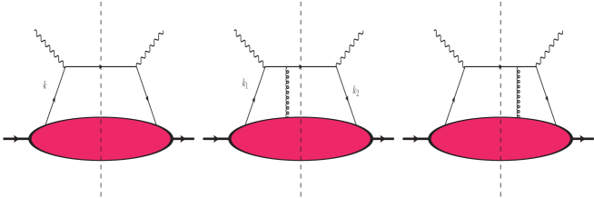
Figure 1: A series of LO diagrams in the diagrammatic method.

We consider a set of the general diagrams shown in Fig. 1 and extract twist-3 contributions from these diagrams. We start from the first diagram in Fig. 1, which can be expressed as

$$w^{\mu\nu}_{1}=\int d^{4}\xi\int{d^{4}k\over(2\pi)^{4}}e^{ik\cdot\xi}\langle pS_{\perp}|\bar{\psi}_{j}(0)\psi_{i}(\xi)|pS_{\perp}\rangle H^{\mu\nu}_{ji}(k)\delta^{2}\left(k_{\perp}-p_{c\perp}\right),$$ (10)

where $k$ and $p_{c}$ are the momenta of the parton from initial state proton and that fragments to the final state observed hadron, respectively, $p_{c\perp}=P_{h\perp}/z$. The hard part at LO is given by

$$H^{\mu\nu}_{ji}(k)=\left[\gamma^{\nu}({\mathchoice{\c@ncel\displaystyle{k}}{\c@ncel\textstyle{k}}{\c@ncel\scriptstyle{k}}{\c@ncel\scriptscriptstyle{k}}}+{\mathchoice{\c@ncel\displaystyle{q}}{\c@ncel\textstyle{q}}{\c@ncel\scriptstyle{q}}{\c@ncel\scriptscriptstyle{q}}})\gamma^{\mu}\right]_{ji}(2\pi)^{4}\delta\left(k^{+}+q^{+}-p_{c}^{+}\right)\delta(k^{-}+q^{-}-p_{c}^{-}).$$ (11)

We perform $P_{h\perp}$-integration before the collinear expansion,

$$\int d^{2}P_{h\perp}\epsilon^{P_{h\perp}S_{\perp}pn}\delta^{2}(k_{\perp}-p_{c\perp})=z^{3}\epsilon^{\alpha S_{\perp}pn}k_{\perp\alpha}.$$ (12)

Because the $P_{h\perp}$-integration gives $O(k_{\perp})$ factor, we can identify the leading term in the collinear expansion as a twist-3 contribution. We perform the collinear expansion of the hard part around $k^{\mu}=(k\cdot n)p^{\mu}\equiv k_{p}^{\mu}$

$$H^{\mu\nu}(k)=H^{\mu\nu}(k_{p})+O(k_{\perp}),$$ (13)

and substitute the above expansion into the hadronic tensor as shown in Eq. (10)

$$\int d^{2}P_{h\perp}\epsilon^{P_{h\perp}S_{\perp}pn}w_{1}^{\mu\nu} = z^{3}\epsilon_{\alpha}^{\ S_{\perp}pn}\int d^{4}\xi\int{d^{4}k\over(2\pi)^{4}}e^{ik\cdot\xi}\langle pS_{\perp}|\bar{\psi}_{j}(0)\psi_{i}(\xi)|pS_{\perp}\rangle k_{\perp}^{\alpha}H^{\mu\nu}_{ji}(k_{p})$$ (14)

$$= iz^{3}\epsilon_{\alpha}^{\ S_{\perp}pn}\int dx\int{d\lambda\over 2\pi}e^{i\lambda x}\langle pS_{\perp}|\bar{\psi}_{j}(0)\partial^{\alpha}\psi_{i}(\lambda)|pS_{\perp}\rangle H^{\mu\nu}_{ji}(xp).$$

Now we turn to the second and the third diagrams in Fig. 1. These two diagrams can be expressed as

$$w_{2}^{\mu\nu} = \int d^{4}\xi_{1}\int d^{4}\xi_{2}\int{d^{4}k_{1}\over(2\pi)^{4}}\int{d^{4}k_{2}\over(2\pi)^{4}}e^{ik_{1}\cdot\xi_{1}}e^{i(k_{2}-k_{1})\cdot\xi_{2}}\langle pS_{\perp}|\bar{\psi}_{j}(0)gA^{\rho}(\xi_{2})\psi_{i}(\xi_{1})|pS_{\perp}\rangle$$ (15)

$$\times\left[H^{\mu\nu}_{L\rho\,ji}(k_{1},k_{2})\delta^{2}(k_{2\perp}-p_{c\perp})+H^{\mu\nu}_{R\rho\,ji}(k_{1},k_{2})\delta^{2}(k_{1\perp}-p_{c\perp})\right],$$

where the hard parts are given by

$$H^{\mu\nu}_{L\rho\,ji}(k_{1},k_{2}) = -\left[\gamma^{\nu}({\mathchoice{\c@ncel\displaystyle{k}}{\c@ncel\textstyle{k}}{\c@ncel\scriptstyle{k}}{\c@ncel\scriptscriptstyle{k}}}_{2}+{\mathchoice{\c@ncel\displaystyle{q}}{\c@ncel\textstyle{q}}{\c@ncel\scriptstyle{q}}{\c@ncel\scriptscriptstyle{q}}})\gamma_{\rho}({\mathchoice{\c@ncel\displaystyle{k}}{\c@ncel\textstyle{k}}{\c@ncel\scriptstyle{k}}{\c@ncel\scriptscriptstyle{k}}}_{1}+{\mathchoice{\c@ncel\displaystyle{q}}{\c@ncel\textstyle{q}}{\c@ncel\scriptstyle{q}}{\c@ncel\scriptscriptstyle{q}}})\gamma^{\mu}\right]_{ji}{1\over(q+k_{1})^{2}+i\epsilon}(2\pi)^{4}\delta(k_{2}^{+}+q^{+}-p_{c}^{+})\delta(k_{2}^{-}+q^{-}-p_{c}^{-}),$$

$$H^{\mu\nu}_{R\rho\,ji}(k_{1},k_{2}) = -\left[\gamma^{\nu}({\mathchoice{\c@ncel\displaystyle{k}}{\c@ncel\textstyle{k}}{\c@ncel\scriptstyle{k}}{\c@ncel\scriptscriptstyle{k}}}_{2}+{\mathchoice{\c@ncel\displaystyle{q}}{\c@ncel\textstyle{q}}{\c@ncel\scriptstyle{q}}{\c@ncel\scriptscriptstyle{q}}})\gamma_{\rho}({\mathchoice{\c@ncel\displaystyle{k}}{\c@ncel\textstyle{k}}{\c@ncel\scriptstyle{k}}{\c@ncel\scriptscriptstyle{k}}}_{1}+{\mathchoice{\c@ncel\displaystyle{q}}{\c@ncel\textstyle{q}}{\c@ncel\scriptstyle{q}}{\c@ncel\scriptscriptstyle{q}}})\gamma^{\mu}\right]_{ji}{1\over(q+k_{2})^{2}-i\epsilon}(2\pi)^{4}\delta(k_{1}^{+}+q^{+}-p_{c}^{+})\delta(k_{1}^{-}+q^{-}-p_{c}^{-}).$$ (16)

The $P_{h\perp}$-integration gives $O(k_{1,2\perp})$ and then the leading term in collinear expansion gives twist-3 contribution again,

$$H^{\mu\nu}_{L(R)\rho\,ji}(k_{1},k_{2})=H^{\mu\nu}_{L(R)\rho\,ji}(k_{1p},k_{2p})+O(k_{1,2\perp}).$$ (17)

For the matrix element, we have to separate the components of the gluon field $A^{\rho}$ into “longitudinal” and “transverse” part as

$$A^{\rho}=A^{n}p^{\rho}+(A^{\rho}-A^{n}p^{\rho}).$$ (18)

The longitudinal part $A^{n}p^{\rho}$ gives the leading contribution. It is straightforward to derive the Ward-Takahashi identities(WTIs) for the hard parts,

$$p^{\rho}H^{\mu\nu}_{L\rho\,ji}(k_{1},k_{2}) = [\gamma^{\nu}(x_{2}{\mathchoice{\c@ncel\displaystyle{p}}{\c@ncel\textstyle{p}}{\c@ncel\scriptstyle{p}}{\c@ncel\scriptscriptstyle{p}}}+{\mathchoice{\c@ncel\displaystyle{q}}{\c@ncel\textstyle{q}}{\c@ncel\scriptstyle{q}}{\c@ncel\scriptscriptstyle{q}}})\gamma^{\mu}]_{ji}{1\over x_{2}-x_{1}-i\epsilon}(2\pi)^{4}{2x_{B}\over Q^{2}}\delta(x_{2}-x_{B})\delta(1-\hat{z})$$

$$= {1\over x_{2}-x_{1}-i\epsilon}H^{\mu\nu}_{ji}(x_{2}p),$$

$$p^{\rho}H^{\mu\nu}_{R\rho\,ji}(k_{1},k_{2}) = -[\gamma^{\nu}(x_{1}{\mathchoice{\c@ncel\displaystyle{p}}{\c@ncel\textstyle{p}}{\c@ncel\scriptstyle{p}}{\c@ncel\scriptscriptstyle{p}}}+{\mathchoice{\c@ncel\displaystyle{q}}{\c@ncel\textstyle{q}}{\c@ncel\scriptstyle{q}}{\c@ncel\scriptscriptstyle{q}}})\gamma^{\mu}]_{ji}{1\over x_{2}-x_{1}-i\epsilon}(2\pi)^{4}{2x_{B}\over Q^{2}}\delta(x_{1}-x_{B})\delta(1-\hat{z})$$ (19)

$$= -{1\over x_{2}-x_{1}-i\epsilon}H^{\mu\nu}_{ji}(x_{1}p).$$

Finally the hadronic tensor shown in Eq. (15) can be expressed as

$$\int d^{2}P_{h\perp}\epsilon^{P_{h\perp}S_{\perp}pn}w_{2}^{\mu\nu}$$ (20)

$$= z^{3}\epsilon_{\alpha}^{\ S_{\perp}pn}\int d^{4}\xi_{1}\int d^{4}\xi_{2}\int{d^{4}k_{1}\over(2\pi)^{4}}\int{d^{4}k_{2}\over(2\pi)^{4}}e^{ik_{1}\cdot\xi_{1}}e^{i(k_{2}-k_{1})\cdot\xi_{2}}\langle pS_{\perp}|\bar{\psi}_{j}(0)gA^{n}(\xi_{2})\psi_{i}(\xi_{1})|pS_{\perp}\rangle$$

$$\times{1\over x_{2}-x_{1}-i\epsilon}\Bigl{[}k^{\alpha}_{2\perp}H^{\mu\nu}_{ji}(x_{2}p)-k^{\alpha}_{1\perp}H^{\mu\nu}_{ji}(x_{1}p)\Bigr{]}$$

$$= z^{3}\epsilon_{\alpha}^{\ S_{\perp}pn}\int d^{4}\xi_{1}\int d^{4}\xi_{2}\int{d^{4}k_{1}\over(2\pi)^{4}}\int{d^{4}k_{2}\over(2\pi)^{4}}e^{ik_{1}\cdot\xi_{1}}e^{i(k_{2}-k_{1})\cdot\xi_{2}}\langle pS_{\perp}|\bar{\psi}_{j}(0)gA^{n}(\xi_{2})\psi_{i}(\xi_{1})|pS_{\perp}\rangle$$

$$\times{1\over x_{2}-x_{1}-i\epsilon}\Bigl{[}(k^{\alpha}_{2\perp}-k^{\alpha}_{1\perp})H^{\mu\nu}_{ji}(x_{2}p)+k^{\alpha}_{1\perp}(H^{\mu\nu}_{ji}(x_{2}p)-H^{\mu\nu}_{ji}(x_{1}p))\Bigr{]}$$

$$= iz^{3}\epsilon_{\alpha}^{\ S_{\perp}pn}\int dx\int{d\lambda\over 2\pi}e^{i\lambda x}\langle pS_{\perp}|\bar{\psi}_{j}(0)ig\int^{\infty}_{\lambda}d\lambda^{\prime}\Bigl{[}\partial^{\alpha}A^{n}(\lambda^{\prime}n)-\partial^{n}A^{\alpha}(\lambda^{\prime}n)\Bigr{]}\psi_{i}(\lambda n)|pS_{\perp}\rangle H^{\mu\nu}_{ji}(xp)$$

$$+iz^{3}\epsilon_{\alpha}^{\ S_{\perp}pn}\int dx\int{d\lambda\over 2\pi}e^{i\lambda x}\langle pS_{\perp}|\bar{\psi}_{j}(0)\Bigl{[}ig\int^{0}_{\lambda}d\lambda^{\prime}A^{n}(\lambda^{\prime}n)\Bigr{]}\partial^{\alpha}\psi_{i}(\lambda n)|pS_{\perp}\rangle H^{\mu\nu}_{ji}(xp)$$

$$-iz^{3}\epsilon_{\alpha}^{\ S_{\perp}pn}\int dx\int{d\lambda\over 2\pi}e^{i\lambda x}\langle pS_{\perp}|\bar{\psi}_{j}(0)igA^{\alpha}(\lambda n)\psi_{i}(\lambda n)|pS_{\perp}\rangle H^{\mu\nu}_{ji}(xp).$$

Combing Eqs. (14) and (20), we can obtain the result

$$\int d^{2}P_{h\perp}\epsilon^{P_{h\perp}S_{\perp}pn}w^{\mu\nu}$$

$$= iz^{3}\epsilon_{\alpha}^{\ S_{\perp}pn}\int dx\int{d\lambda\over 2\pi}e^{i\lambda x}\langle pS_{\perp}|\bar{\psi}_{j}(0)\Bigl{(}D^{\alpha}(\lambda n)\psi_{i}(\lambda n)+ig\int^{0}_{\lambda}d\lambda^{\prime}A^{n}(\lambda^{\prime}n)\partial^{\alpha}\psi_{i}(\lambda n)\Bigl{)}|pS_{\perp}\rangle H^{\mu\nu}_{ji}(xp)$$ (21)

$$+iz^{3}\epsilon_{\alpha}^{\ S_{\perp}pn}\int dx\int{d\lambda\over 2\pi}e^{i\lambda x}\langle pS_{\perp}|\bar{\psi}_{j}(0)ig\int^{\infty}_{\lambda}d\lambda^{\prime}\Bigl{(}\partial^{\alpha}A^{n}(\lambda^{\prime}n)-\partial^{n}A^{\alpha}(\lambda^{\prime}n)\Bigr{)}\psi_{i}(\lambda n)|pS_{\perp}\rangle H^{\mu\nu}_{ji}(xp).$$

We can find that this matrix element corresponds to $O(g)$ term in the first moment of the TMD correlator

$$\int d^{2}p_{T}\,p_{T}^{\alpha}\Bigl{(}\int{d\lambda\over 2\pi}\int{dx_{T}\over 2\pi}e^{i\lambda x}e^{ix_{T}\cdot p_{T}}\langle pS_{\perp}|\bar{\psi}_{j}(0)[0,\infty n][\infty n,\infty n+x_{T}][\infty n+x_{T},\lambda n+x_{T}]\psi_{i}(\lambda n+x_{T})|pS_{\perp}\rangle\Bigr{)}$$ (22)

$$= i\int{d\lambda\over 2\pi}e^{i\lambda x}\langle pS_{\perp}|\bar{\psi}_{j}(0)[0,\lambda n]D^{\alpha}(\lambda n)\psi_{i}(\lambda n)|pS_{\perp}\rangle$$

$$+i\int{d\lambda\over 2\pi}e^{i\lambda x}\int^{\infty}_{\lambda}d\lambda^{\prime}\langle pS_{\perp}|\bar{\psi}_{j}(0)[0,\lambda^{\prime}n]igF^{\alpha n}(\lambda^{\prime}n)[\lambda^{\prime}n,\lambda n]\psi_{i}(\lambda n)|pS_{\perp}\rangle$$

$$= -\pi{M_{N}\over 4}\epsilon^{\alpha pnS_{\perp}}G_{q,F}(x,x)+\cdots,$$

where $[\cdots]$ represents the Wilson line, $M_{N}$ is the nucleon mass and we used the fact that the first moment of the TMD Sivers function gives the Qiu-Sterman function $G_{q,F}(x,x)$. The nonlinear term in the field strength tensor $F^{\alpha+}$ and the higher order terms in the Wilson lines which have to be added to Eq. (21) come from the more gluon-linked diagrams in Fig. 2. Finally we can derive the LO cross section formula as

$${d\langle P_{h\perp}\Delta\sigma\rangle^{\rm LO}\over dx_{B}dydz_{h}}=\tilde{\sigma}_{0}\sum_{q}e^{2}_{q}G_{q,F}(x_{B},x_{B})D_{q\to h}(z_{h}).$$ (23)

where $\tilde{\sigma}_{0}=-\pi M_{N}\sigma_{0}$. As we demonstrated here, the LO cross section for the weighted SSA is proportional to the first moment of the TMD function(also known as the kinematical twist-3 function). We can expect the NLO contribution gives the evolution equation to the twist-3 Qiu-Sterman function, $G_{q,F}(x,x)$ in this case. This technique is quite general so that we can apply the same technique to other TMD functions. When we focus on the twist-3 fragmentation effect, we can derive the evolution equation for the first Moment of the Collins function. When we consider the double spin asymmetry $A_{LT}$ and change the weight factor $\epsilon^{ij}P_{h\perp i}S_{\perp j}\to(P_{h}\cdot S_{\perp})$, we can investigate other TMD distribution functions like the Worm-Gear and the Pretzelosity.

III Transverse-momentum-weighted SSA at NLO

In this section, we review the calculation for transverse-momentum-weighted SSA at NLO including both real and virtual corrections.

III.1 Virtual correction

We first consider the NLO contribution from the virtual correction which is given by the $2\to 1$ scattering amplitude with one gluon loop. When we adopt the dimensional regularization scheme, the gauge-invariance of the cross section is maintained for the loop diagram. Then we can derive the same WTI as shown in Eq. (19) which is the consequence of gauge-invariance of the diagrams. Taking advantage of this fact, we just need to calculate simple diagrams shown in Fig. 2 for the virtual correction.

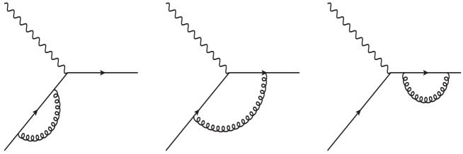
Figure 2: The NLO virtual correction diagrams in SIDIS.

The calculation for this kind of one-loop diagrams have been well established, which is exactly the same as the vertex correction at leading twist. We follow the conventional technique here. All ultraviolet divergences can be canceled by the renormalization of the QCD Lagrangian. Then we can set the ultraviolet and infrared divergences are the same with each other in dimensions regularization approach, $\epsilon_{\rm UV}=\epsilon_{\rm IR}$, and identify all divergences as infrared. In this definition, we don’t have to think about the first and the third amplitudes in Fig. 2 because these are exactly zero in the mass case as we considered here. The hard partonic cross section with the second amplitude is given by

$$\Bigl{(}-{1\over 1-\epsilon}g_{\mu\nu}\Bigr{)}C_{F}g^{2}\mu^{2\epsilon}\int{d^{D}\ell\over(2\pi)^{D}i}{\rm Tr}[x{\mathchoice{\c@ncel\displaystyle{p}}{\c@ncel\textstyle{p}}{\c@ncel\scriptstyle{p}}{\c@ncel\scriptscriptstyle{p}}}\gamma^{\nu}{{\mathchoice{\c@ncel\displaystyle{p}}{\c@ncel\textstyle{p}}{\c@ncel\scriptstyle{p}}{\c@ncel\scriptscriptstyle{p}}}_{c}}\gamma^{\rho}({{\mathchoice{\c@ncel\displaystyle{p}}{\c@ncel\textstyle{p}}{\c@ncel\scriptstyle{p}}{\c@ncel\scriptscriptstyle{p}}}_{c}}-{\mathchoice{\c@ncel\displaystyle{\ell}}{\c@ncel\textstyle{\ell}}{\c@ncel\scriptstyle{\ell}}{\c@ncel\scriptscriptstyle{\ell}}})\gamma^{\mu}(x{\mathchoice{\c@ncel\displaystyle{p}}{\c@ncel\textstyle{p}}{\c@ncel\scriptstyle{p}}{\c@ncel\scriptscriptstyle{p}}}-{\mathchoice{\c@ncel\displaystyle{\ell}}{\c@ncel\textstyle{\ell}}{\c@ncel\scriptstyle{\ell}}{\c@ncel\scriptscriptstyle{\ell}}})\gamma_{\rho}]{1\over\ell^{2}({p_{c}}-\ell)^{2}(xp-\ell)^{2}}$$ (24)

$$= C_{F}g^{2}\mu^{2\epsilon}\int{d^{D}\ell\over(2\pi)^{D}i}\left[-4{1\over({p_{c}}-\ell)^{2}(xp-\ell)^{2}}\left({3\over 2}+\epsilon\right)Q^{2}+{4Q^{2}\over\ell^{2}(p_{c}-\ell)^{2}(xp-\ell)^{2}}\right],$$

where $\epsilon={4-D\over 2}$ in $D$-dimension, we made a change $g_{\mu\nu}\to{1\over 1-\epsilon}g_{\mu\nu}$ for $D$-dimensional calculation, and we used the fact that

$$\int{d^{D}\ell\over(2\pi)^{D}i}{1\over\ell^{2}}=\int{d^{D}\ell\over(2\pi)^{D}i}{1\over(xp-\ell)^{2}}=\int{d^{D}\ell\over(2\pi)^{D}i}{1\over\ell^{2}({p_{c}}-\ell)^{2}}=\int{d^{D}\ell\over(2\pi)^{D}i}{1\over\ell^{2}(xp-\ell)^{2}}=0.$$ (25)

We perform the basic $D$-dimensional calculation for each integration,

$$\int{d^{D}\ell\over(2\pi)^{D}i}{1\over({p_{c}}-\ell)^{2}(xp-\ell)^{2}} = {1\over 16\pi^{2}}\Bigl{(}{4\pi\over Q^{2}}\Bigr{)}^{\epsilon}{1\over\Gamma(1-\epsilon)}\Gamma(1-\epsilon)\Gamma(\epsilon)B(1-\epsilon,1-\epsilon)$$ (26)

$$= {1\over 16\pi^{2}}\Bigl{(}{4\pi\over Q^{2}}\Bigr{)}^{\epsilon}{1\over\Gamma(1-\epsilon)}\Bigl{(}{1\over\epsilon}+2+O(\epsilon)\Bigr{)},$$

$$\int{d^{D}\ell\over(2\pi)^{D}i}{1\over\ell^{2}({p_{c}}-\ell)^{2}(xp-\ell)^{2}} = -{1\over 16\pi^{2}Q^{2}}\Bigl{(}{4\pi\over Q^{2}}\Bigr{)}^{\epsilon}{1\over\Gamma(1-\epsilon)}\Gamma(1-\epsilon)\Gamma(1+\epsilon)B(1,-\epsilon)B(-\epsilon,1-\epsilon)$$ (27)

$$= -{1\over 16\pi^{2}Q^{2}}\Bigl{(}{4\pi\over Q^{2}}\Bigr{)}^{\epsilon}{1\over\Gamma(1-\epsilon)}\Bigl{(}{1\over\epsilon^{2}}+O(\epsilon)\Bigr{)}.$$

The complex-conjugate diagram gives the same contribution. Then we can show the cross section for the NLO virtual correction as

$${d\langle P_{h\perp}\Delta\sigma\rangle^{\rm virtual}\over dx_{B}dydz_{h}}=\tilde{\sigma}_{0}{\alpha_{s}\over 2\pi}\sum_{q}e_{q}^{2}G_{q,F}(x_{B},x_{B})D_{q\to h}(z_{h})C_{F}\Bigr{(}{4\pi\mu^{2}\over Q^{2}}\Bigr{)}^{\epsilon}{1\over\Gamma(1-\epsilon)}\Bigl{(}-{2\over\epsilon^{2}}-{3\over\epsilon}-8\Bigr{)},$$ (28)

this is exactly the same as the virtual correction at leading twist. The strategy in the virtual correction calculation presented here is different with that shown in Ref. Kang:2012ns , in which the authors didn’t use the WTI shown in Eq. (19) and directly calculated $H^{\mu\nu}_{L(R)\rho\,ji}(k_{1},k_{2})$ which has one more external gluon line with the momentum $k_{2}-k_{1}$ in Fig. 2. The authors obtained a consistent result with Eq. (28), which demonstrated the validation of WTI through explicit calculation by including all virtual diagrams shown in Figs. 3, 4 in Ref. Kang:2012ns . We would like to comment that the WTI reduces much calculational cost. The direct calculation of $H^{\mu\nu}_{L(R)\rho\,ji}(k_{1},k_{2})$ takes tremendous time as they contain significant amount of tensor reduction and integration. These two calculations should be conceptually the same with each other as long as we correctly keep track of all imaginary contributions. We confirmed in this section the consistency mathematically in $2\to 1$-scattering case. The consistency check in a more general way will be a future task in the collinear twist-3 factorization approach.

III.2 Real correction

We now complete the NLO calculation by adding the real emission contribution represented by $2\to 2$ partonic scattering process. The calculation for $2\to 2$ scattering diagrams have been well studied in $P_{h\perp}$-unintegrated case. We just have to repeat the same calculation but in $D$-dimension. We adopt the conventional technique by separating the propagator into the principle value part and imaginary part qiu ; Kanazawa:2000cx ; koike ; Koike:2011mb ,

$${1\over k^{2}+i\epsilon}\to P{1\over k^{2}}-i\pi\delta(k^{2}),$$ (29)

and we focus on the pole contribution $-i\delta(k^{2})$ which is required to generate the phase space for SSA. The derivation of the cross section for the pole contribution has been well developed so far based on the diagrammatic method we reviewed in Sec. 2. Here we recall the result derived in Ref. koike as

$$w^{\mu\nu} = i\int dx_{1}\int dx_{2}\,M^{\alpha}_{ij\,F}(x_{1},x_{2})p^{\beta}{\partial\over\partial k_{2}^{\alpha}}\Bigl{(}H^{{\rm pole}\,\mu\nu}_{Lji\,\beta}(k_{1},k_{2})+H^{{\rm pole}\,\mu\nu}_{Rji\,\beta}(k_{1},k_{2})\Bigr{)}\Bigr{|}_{k_{i}=x_{i}p},$$ (30)

where the matrix element $M^{\alpha}_{ij\,F}$ is given by

$$M^{\alpha}_{ij\,F}(x_{1},x_{2}) = \int{d\lambda\over 2\pi}\int{d\lambda^{\prime}\over 2\pi}e^{i\lambda x_{1}}e^{i\lambda^{\prime}(x_{2}-x_{1})}\langle pS_{\perp}|\bar{\psi}_{j}(0)gF^{\alpha n}(\lambda^{\prime}n)\psi_{i}(\lambda n)|pS_{\perp}\rangle$$ (31)

$$= {M_{N}\over 4}\left[\epsilon^{\alpha pnS_{\perp}}({\mathchoice{\c@ncel\displaystyle{p}}{\c@ncel\textstyle{p}}{\c@ncel\scriptstyle{p}}{\c@ncel\scriptscriptstyle{p}}})_{ij}G_{q,F}(x_{1},x_{2})+iS^{\alpha}_{\perp}(\gamma_{5}{\mathchoice{\c@ncel\displaystyle{p}}{\c@ncel\textstyle{p}}{\c@ncel\scriptstyle{p}}{\c@ncel\scriptscriptstyle{p}}})_{ij}\tilde{G}_{q,F}(x_{1},x_{2})\right]+\cdots.$$

We can construct the gauge-invariant expression (30) before performing the $p_{h}$-integration. There are three types of pole contributions in SIDIS which are respectively known as soft-gluon pole contribution(SGP, $x_{1}=x_{2}=x$), hard pole contribution(HP, $x_{1}=x,\ x_{2}=x_{B}$ or $x_{1}=x_{B},\ x_{2}=x$) and another hard pole contribution(HP2, $x_{1}=x_{B},\ x_{2}=x_{B}-x$ or $x_{2}=x_{B},\ x_{1}=x_{B}-x$ ) koike ; Yoshida:2016tfh , the corresponding hard parts are given by

$$H^{{\rm pole}\,\mu\nu}_{Lji\,\beta} = H^{{\rm SGP}\,\mu\nu}_{Lji\,\beta}(k_{1},k_{2})\Bigl{\{}-i\pi\delta\Bigl{[}({p_{c}}-(k_{2}-k_{1}))^{2}\Bigr{]}\Bigr{\}}(2\pi)\delta\Bigl{[}(k_{2}+q-{p_{c}})^{2}\Bigr{]}$$

$$+H^{{\rm HP}\,\mu\nu}_{Lji\,\beta}(k_{1},k_{2})\Bigl{\{}-i\pi\delta\Bigl{[}(k_{1}+q)^{2}\Bigr{]}\Bigr{\}}(2\pi)\delta\Bigl{[}(k_{2}+q-{p_{c}})^{2}\Bigr{]}$$

$$+H^{{\rm HP2}\,\mu\nu}_{Lji\,\beta}(k_{1},k_{2})\Bigl{\{}i\pi\delta\Bigl{[}(k_{2}+q)^{2}\Bigr{]}\Bigr{\}}(2\pi)\delta\Bigl{[}(k_{2}-k_{1}+q-{p_{c}})^{2}\Bigr{]},$$

$$H^{{\rm pole}\,\mu\nu}_{Rji\,\beta} = H^{{\rm SGP}\,\mu\nu}_{Rji\,\beta}(k_{1},k_{2})\Bigl{\{}i\pi\delta\Bigl{[}({p_{c}}+(k_{2}-k_{1})]^{2}\Bigr{)}\Bigr{\}}(2\pi)\delta\Bigl{[}(k_{1}+q-{p_{c}})^{2}\Bigr{]}$$ (32)

$$+H^{{\rm HP}\,\mu\nu}_{Rji\,\beta}(k_{1},k_{2})\Bigl{\{}i\pi\delta\Bigl{[}(k_{2}+q)^{2}\Bigr{]}\Bigr{\}}(2\pi)\delta\Bigl{[}(k_{1}+q-{p_{c}})^{2}\Bigr{]}$$

$$+H^{{\rm HP2}\,\mu\nu}_{Rji\,\beta}(k_{1},k_{2})\Bigl{\{}-i\pi\delta\Bigl{[}(k_{1}+q)^{2}\Bigr{]}\Bigr{\}}(2\pi)\delta\Bigl{[}(k_{1}-k_{2}+q-{p_{c}})^{2}\Bigr{]}.$$

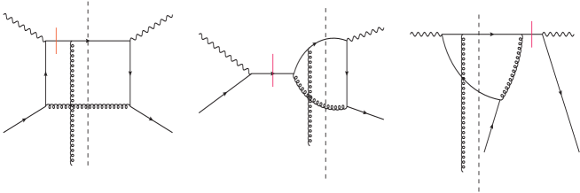
Figure 3: Typical diagrams for soft-gluon pole(left), hard pole(middle) and another hard pole(right). The red barred propagator gives the pole term.

Typical diagrams for each pole contribution are shown in Fig. 3 (full diagrams can be found in Yoshida:2016tfh ). We write down the explicit form of each diagram in Fig. 3 in order to help readers to follow our calculation,

$$(H^{{\rm SGP}\,\mu\nu}_{Lji\,\beta}(k_{1},k_{2}))_{\rm Fig.\ref{pole}}$$ (33)

$$= -[\gamma^{\sigma}({\mathchoice{\c@ncel\displaystyle{p}}{\c@ncel\textstyle{p}}{\c@ncel\scriptstyle{p}}{\c@ncel\scriptscriptstyle{p}}}_{c}-{\mathchoice{\c@ncel\displaystyle{q}}{\c@ncel\textstyle{q}}{\c@ncel\scriptstyle{q}}{\c@ncel\scriptscriptstyle{q}}})\gamma^{\nu}{\mathchoice{\c@ncel\displaystyle{p}}{\c@ncel\textstyle{p}}{\c@ncel\scriptstyle{p}}{\c@ncel\scriptscriptstyle{p}}}_{c}\gamma_{\beta}({\mathchoice{\c@ncel\displaystyle{p}}{\c@ncel\textstyle{p}}{\c@ncel\scriptstyle{p}}{\c@ncel\scriptscriptstyle{p}}}_{c}-{\mathchoice{\c@ncel\displaystyle{k}}{\c@ncel\textstyle{k}}{\c@ncel\scriptstyle{k}}{\c@ncel\scriptscriptstyle{k}}}_{2}+{\mathchoice{\c@ncel\displaystyle{k}}{\c@ncel\textstyle{k}}{\c@ncel\scriptstyle{k}}{\c@ncel\scriptscriptstyle{k}}}_{1})\gamma^{\mu}({\mathchoice{\c@ncel\displaystyle{p}}{\c@ncel\textstyle{p}}{\c@ncel\scriptstyle{p}}{\c@ncel\scriptscriptstyle{p}}}_{c}-{\mathchoice{\c@ncel\displaystyle{k}}{\c@ncel\textstyle{k}}{\c@ncel\scriptstyle{k}}{\c@ncel\scriptscriptstyle{k}}}_{2}+{\mathchoice{\c@ncel\displaystyle{k}}{\c@ncel\textstyle{k}}{\c@ncel\scriptstyle{k}}{\c@ncel\scriptscriptstyle{k}}}_{1}-{\mathchoice{\c@ncel\displaystyle{q}}{\c@ncel\textstyle{q}}{\c@ncel\scriptstyle{q}}{\c@ncel\scriptscriptstyle{q}}})\gamma^{\rho}]_{ji}{1\over(p_{c}-q)^{2}}{1\over(p_{c}-k_{2}+k_{1}-q)^{2}}[-g_{\perp\rho\sigma}(k_{2}+q-p_{c})],$$

$$(H^{{\rm HP}\,\mu\nu}_{Lji\,\beta}(k_{1},k_{2}))_{\rm Fig.\ref{pole}}$$

$$= -[\gamma^{\sigma}({\mathchoice{\c@ncel\displaystyle{p}}{\c@ncel\textstyle{p}}{\c@ncel\scriptstyle{p}}{\c@ncel\scriptscriptstyle{p}}}_{c}-{\mathchoice{\c@ncel\displaystyle{q}}{\c@ncel\textstyle{q}}{\c@ncel\scriptstyle{q}}{\c@ncel\scriptscriptstyle{q}}})\gamma^{\nu}{\mathchoice{\c@ncel\displaystyle{p}}{\c@ncel\textstyle{p}}{\c@ncel\scriptstyle{p}}{\c@ncel\scriptscriptstyle{p}}}_{c}\gamma_{\beta}({\mathchoice{\c@ncel\displaystyle{p}}{\c@ncel\textstyle{p}}{\c@ncel\scriptstyle{p}}{\c@ncel\scriptscriptstyle{p}}}_{c}-{\mathchoice{\c@ncel\displaystyle{k}}{\c@ncel\textstyle{k}}{\c@ncel\scriptstyle{k}}{\c@ncel\scriptscriptstyle{k}}}_{2}+{\mathchoice{\c@ncel\displaystyle{k}}{\c@ncel\textstyle{k}}{\c@ncel\scriptstyle{k}}{\c@ncel\scriptscriptstyle{k}}}_{1})\gamma^{\rho}({\mathchoice{\c@ncel\displaystyle{k}}{\c@ncel\textstyle{k}}{\c@ncel\scriptstyle{k}}{\c@ncel\scriptscriptstyle{k}}}_{1}+{\mathchoice{\c@ncel\displaystyle{q}}{\c@ncel\textstyle{q}}{\c@ncel\scriptstyle{q}}{\c@ncel\scriptscriptstyle{q}}})\gamma^{\mu}]_{ji}{1\over(p_{c}-q)^{2}}{1\over(p_{c}-k_{2}+k_{1})^{2}}[-g_{\perp\rho\sigma}(k_{2}+q-p_{c})],$$

$$(H^{{\rm HP2}\,\mu\nu}_{Lji\,\beta}(k_{1},k_{2}))_{\rm Fig.\ref{pole}}$$

$$= [\gamma^{\nu}({\mathchoice{\c@ncel\displaystyle{k}}{\c@ncel\textstyle{k}}{\c@ncel\scriptstyle{k}}{\c@ncel\scriptscriptstyle{k}}}_{2}+{\mathchoice{\c@ncel\displaystyle{q}}{\c@ncel\textstyle{q}}{\c@ncel\scriptstyle{q}}{\c@ncel\scriptscriptstyle{q}}})\gamma^{\rho}{\mathchoice{\c@ncel\displaystyle{p}}{\c@ncel\textstyle{p}}{\c@ncel\scriptstyle{p}}{\c@ncel\scriptscriptstyle{p}}}_{c}\gamma_{\beta}({\mathchoice{\c@ncel\displaystyle{p}}{\c@ncel\textstyle{p}}{\c@ncel\scriptstyle{p}}{\c@ncel\scriptscriptstyle{p}}}_{c}-{\mathchoice{\c@ncel\displaystyle{k}}{\c@ncel\textstyle{k}}{\c@ncel\scriptstyle{k}}{\c@ncel\scriptscriptstyle{k}}}_{2}+{\mathchoice{\c@ncel\displaystyle{k}}{\c@ncel\textstyle{k}}{\c@ncel\scriptstyle{k}}{\c@ncel\scriptscriptstyle{k}}}_{1})\gamma^{\mu}({\mathchoice{\c@ncel\displaystyle{p}}{\c@ncel\textstyle{p}}{\c@ncel\scriptstyle{p}}{\c@ncel\scriptscriptstyle{p}}}_{c}-{\mathchoice{\c@ncel\displaystyle{k}}{\c@ncel\textstyle{k}}{\c@ncel\scriptstyle{k}}{\c@ncel\scriptscriptstyle{k}}}_{2}+{\mathchoice{\c@ncel\displaystyle{k}}{\c@ncel\textstyle{k}}{\c@ncel\scriptstyle{k}}{\c@ncel\scriptscriptstyle{k}}}_{1}-{\mathchoice{\c@ncel\displaystyle{q}}{\c@ncel\textstyle{q}}{\c@ncel\scriptstyle{q}}{\c@ncel\scriptscriptstyle{q}}})\gamma_{\rho}]_{ji}{1\over(p_{c}-k_{2}-q)^{2}}{1\over(p_{c}-k_{2}+k_{1})^{2}},$$

where $g_{\perp\rho\sigma}$ is the sum of the polarization vector $\sum_{r}\epsilon_{r\rho}(k)\epsilon_{r\sigma}(k)=-g_{\perp\rho\sigma}(k)$. We can show the WTI for the pole diagrams

$$(k_{2}-k_{1})^{\beta}{H^{{\rm pole}\,\mu\nu}_{L(R)ji\,\beta}(k_{1},k_{2})}=0,$$ (34)

and it gives a useful relation

$$p^{\beta}{\partial\over\partial k_{2}^{\alpha}}H^{{\rm pole}\,\mu\nu}_{L(R)ji\,\beta}(k_{1},k_{2})\Bigr{|}_{k_{i}=x_{i}p}=-{1\over x_{2}-x_{1}-i\epsilon}H^{{\rm pole}\,\mu\nu}_{L(R)ji\,\alpha}(k_{1},k_{2}).$$ (35)

For HP and HP2 contributions, we can use Eq. (35) and don’t have to perform $k_{2}$-derivative directly as in Eq. (30). However, we can’t use this relation for SGP contribution because it contains a delta function $\delta(x_{1}-x_{2})$. In Ref. Koike:2006qv , the authors found a reduction formula for SGP contribution as

$$p^{\beta}{\partial\over\partial k_{2}^{\alpha}}\Bigl{(}H^{{\rm SGP}\,\mu\nu}_{Lji\,\beta}(k_{1},k_{2})+H^{{\rm SGP}\,\mu\nu}_{Rji\,\beta}(k_{1},k_{2})\Bigr{)}={1\over 2NC_{F}}{1\over x_{2}-x_{1}-i\epsilon}\left({\partial\over\partial p_{c}^{\alpha}}-{p_{c\alpha}p^{\mu}\over p_{c}\cdot p}{\partial\over\partial p_{c}^{\mu}}\right)H(xp),$$ (36)

where $H(xp)$ is the $2\to 2$-scattering cross section without the external gluon line with momentum $(x_{2}-x_{1})p$. Substituting Eq. (31) into Eq. (30) and using Eqs. (35, 36), we can derive the following result,

$$w^{\mu\nu} = {M_{N}\pi^{2}\over 2}\int{dx\over x}\delta\Bigl{[}(xp+q-p_{c})^{2}\Bigr{]}\Bigl{[}-2\Bigl{(}(\hat{s}+Q^{2})\epsilon^{p_{c}pnS_{\perp}}+\hat{u}\epsilon^{qpnS_{\perp}}\Bigr{)}{d\over dx}G_{q,F}(x,x){1\over\hat{t}\hat{u}}{\rm Tr}[x{\mathchoice{\c@ncel\displaystyle{p}}{\c@ncel\textstyle{p}}{\c@ncel\scriptstyle{p}}{\c@ncel\scriptscriptstyle{p}}}H(xp)]$$ (37)

$$-2\Bigl{[}(\hat{s}+Q^{2})\epsilon^{p_{c}pnS_{\perp}}+\hat{u}\epsilon^{qpnS_{\perp}}\Bigr{]}G_{q,F}(x,x){1\over\hat{t}\hat{u}}\Bigl{\{}Q^{2}\Bigl{(}{\partial\over\partial\hat{s}}-{\partial\over\partial Q^{2}}\Bigr{)}{\rm Tr}[x{\mathchoice{\c@ncel\displaystyle{p}}{\c@ncel\textstyle{p}}{\c@ncel\scriptstyle{p}}{\c@ncel\scriptscriptstyle{p}}}H(xp)]-{\rm Tr}[x{\mathchoice{\c@ncel\displaystyle{p}}{\c@ncel\textstyle{p}}{\c@ncel\scriptstyle{p}}{\c@ncel\scriptscriptstyle{p}}}H(xp)]\Bigr{\}}$$

$$+G_{q,F}(x,x_{B}){1\over\hat{x}-1}{\hat{x}\over Q^{2}}\epsilon_{\alpha}^{\ pnS_{\perp}}\Bigl{[}{\rm Tr}[x{\mathchoice{\c@ncel\displaystyle{p}}{\c@ncel\textstyle{p}}{\c@ncel\scriptstyle{p}}{\c@ncel\scriptscriptstyle{p}}}H_{L}^{{\rm HP}\,\alpha}(x_{B}p,xp)]+{\rm Tr}[x{\mathchoice{\c@ncel\displaystyle{p}}{\c@ncel\textstyle{p}}{\c@ncel\scriptstyle{p}}{\c@ncel\scriptscriptstyle{p}}}H_{R}^{{\rm HP}\,\alpha}(xp,x_{B}p)]\Bigr{]}$$

$$-\tilde{G}_{q,F}(x,x_{B}){1\over\hat{x}-1}{\hat{x}\over Q^{2}}iS_{\perp\alpha}\Bigl{[}{\rm Tr}[\gamma_{5}x{\mathchoice{\c@ncel\displaystyle{p}}{\c@ncel\textstyle{p}}{\c@ncel\scriptstyle{p}}{\c@ncel\scriptscriptstyle{p}}}H_{L}^{{\rm HP}\,\alpha}(x_{B}p,xp)]-{\rm Tr}[\gamma_{5}x{\mathchoice{\c@ncel\displaystyle{p}}{\c@ncel\textstyle{p}}{\c@ncel\scriptstyle{p}}{\c@ncel\scriptscriptstyle{p}}}H_{R}^{{\rm HP}\,\alpha}(xp,x_{B}p)]\Bigr{]}$$

$$+G_{q,F}(x_{B},x_{B}-x){\hat{x}\over Q^{2}}\epsilon_{\alpha}^{\ pnS_{\perp}}\Bigl{[}{\rm Tr}[x{\mathchoice{\c@ncel\displaystyle{p}}{\c@ncel\textstyle{p}}{\c@ncel\scriptstyle{p}}{\c@ncel\scriptscriptstyle{p}}}H_{L}^{{\rm HP2}\,\alpha}((x_{B}-x)p,x_{B}p)]+{\rm Tr}[x{\mathchoice{\c@ncel\displaystyle{p}}{\c@ncel\textstyle{p}}{\c@ncel\scriptstyle{p}}{\c@ncel\scriptscriptstyle{p}}}H_{R}^{{\rm HP2}\,\alpha}(x_{B}p,(x_{B}-x)p)]\Bigr{]}$$

$$-\tilde{G}_{q,F}(x_{B},x_{B}-x){\hat{x}\over Q^{2}}iS_{\perp\alpha}\Bigl{[}{\rm Tr}[\gamma_{5}x{\mathchoice{\c@ncel\displaystyle{p}}{\c@ncel\textstyle{p}}{\c@ncel\scriptstyle{p}}{\c@ncel\scriptscriptstyle{p}}}H_{L}^{{\rm HP2}\,\alpha}((x_{B}-x)p,x_{B}p)]-{\rm Tr}[\gamma_{5}x{\mathchoice{\c@ncel\displaystyle{p}}{\c@ncel\textstyle{p}}{\c@ncel\scriptstyle{p}}{\c@ncel\scriptscriptstyle{p}}}H_{R}^{{\rm HP2}\,\alpha}(x_{B}p,(x_{B}-x)p)]\Bigr{)}\Bigr{]},$$

where we used the Mandelstam variables

$$\hat{s} = (xp+q)^{2}={1-\hat{x}\over\hat{x}}Q^{2},$$ (38)

$$\hat{t} = (p_{c}-q)^{2}=-{1-\hat{z}\over\hat{x}}Q^{2},$$ (39)

$$\hat{u} = (xp-p_{c})^{2}=-{\hat{z}\over\hat{x}}Q^{2},$$ (40)

with $\hat{x}={x_{B}\over x}$, $\hat{z}={z_{h}\over z}$. Then the cross section can be written as

$${d^{4}\langle P_{h\perp}\Delta\sigma\rangle^{\rm real}\over dx_{B}dydz_{h}}$$ (41)

$$\sim \mu^{2\epsilon}\sum_{q}e^{2}_{q}\int{dz}D_{q\to h}(z)\int{d^{2-2\epsilon}p_{c\perp}\over(2\pi)^{2-2\epsilon}}\Bigl{[}\int{dx\over x}\delta\left(p^{2}_{c\perp}-{(1-\hat{x})(1-\hat{z})\hat{z}\over\hat{x}}Q^{2}\right)$$

$$\times{1\over 1-\epsilon}\Bigl{[}{d\over dx}G_{q,F}(x,x)H_{D}+G_{q,F}(x,x)H_{ND}+G_{q,F}(x,x_{B})H_{HP}+\tilde{G}_{q,F}(x,x_{B})H_{HPT}$$

$$+G_{q,F}(x_{B},x_{B}-x)H_{HP2}+\tilde{G}_{q,F}(x_{B},x_{B}-x)H_{HPT2}\Bigr{]},$$

where we used the symmetry of the $P_{h\perp}$-integration as

$$\int d^{2-2\epsilon}P_{h\perp}\,P_{h\perp\alpha}P_{h\perp\beta}\epsilon^{\rho\alpha pn}\epsilon^{\beta pn\sigma} = -\int d^{2-2\epsilon}P_{h\perp}\,{1\over 2(1-\epsilon)}P^{2}_{h\perp}g_{\perp\alpha\beta}\epsilon^{\rho\alpha pn}\epsilon^{\beta pn\sigma}.$$ (42)

The authors of Kang:2012ns found that the factor $1-\epsilon$ in the denominator is essential to derive the correct evolution function of $G_{q,F}(x,x)$. They calculated all SGP and HP contributions associated with $G_{q,F}$. After that, the HP2 contribution and all $\tilde{G}_{q,F}$ contributions were calculated in Yoshida:2016tfh . The results of all hard cross sections are listed in Yoshida:2016tfh . We perform the $p_{c\perp}$-integration,

$$\int{d^{2-2\epsilon}p_{c\perp}\over(2\pi)^{2-2\epsilon}}\delta\Bigl{[}p^{2}_{c\perp}-{(1-\hat{x})(1-\hat{z})\hat{z}\over\hat{x}}Q^{2}\Bigr{]}$$ (43)

$$= {1\over(2\pi)^{2-2\epsilon}}\int{dp_{c\perp}}\int d\Omega_{2-2\epsilon}(p_{c\perp})^{1-2\epsilon}\delta\Bigl{[}p^{2}_{c\perp}-{(1-\hat{x})(1-\hat{z})\hat{z}\over\hat{x}}Q^{2}\Bigr{]}$$

$$= {1\over 4\pi}\Bigl{(}{4\pi\over Q^{2}}\Bigr{)}^{\epsilon}{1\over\Gamma(1-\epsilon)}\Bigl{[}{(1-\hat{x})(1-\hat{z})\hat{z}\over\hat{x}}\Bigr{]}^{-\epsilon},$$

where $\Omega_{2-2\epsilon}$ is the solid angle and it can be integrated out as

$$\int d\Omega_{2-2\epsilon}={2\pi^{1-\epsilon}\over\Gamma(1-\epsilon)}.$$ (44)

We carry out the $\epsilon$-expansion as follows.

$$\hat{z}^{-\epsilon} \simeq 1-\epsilon\ln\hat{z},$$ (45)

$$\hat{x}^{\epsilon} \simeq 1+\epsilon\ln\hat{x},$$ (46)

$$(1-\hat{z})^{-1-\epsilon} \simeq -{1\over\epsilon}\delta(1-\hat{z})+{1\over(1-\hat{z})_{+}}-\epsilon\Bigl{[}{\ln(1-\hat{z})\over 1-\hat{z}}\Bigr{]}_{+},$$ (47)

$$(1-\hat{x})^{-1-\epsilon} \simeq -{1\over\epsilon}\delta(1-\hat{x})+{1\over(1-\hat{x})_{+}}-\epsilon\Bigl{[}{\ln(1-\hat{x})\over 1-\hat{x}}\Bigr{]}_{+}.$$ (48)

Then the cross section can be derived as follows

$${d\langle P_{h\perp}\Delta\sigma\rangle^{\rm real}\over dx_{B}dydz_{h}}$$ (49)

$$= \tilde{\sigma}_{0}{\alpha_{s}\over 2\pi}\Bigl{(}{4\pi\mu^{2}\over Q^{2}}\Bigr{)}^{\epsilon}{1\over\Gamma(1-\epsilon)}\sum_{q}e_{q}^{2}\Biggl{[}C_{F}{2\over\epsilon^{2}}G_{q,F}(x_{B},x_{B})D_{q\to h}(z_{h})$$

$$+\Bigl{(}-{1\over\epsilon}\Bigr{)}\Biggl{\{}D_{q\to h}(z_{h})\Bigl{\{}\int^{1}_{x_{B}}{dx\over x}\Bigl{[}C_{F}{1+\hat{x}^{2}\over(1-\hat{x})_{+}}G_{q,F}(x,x)+{N\over 2}\Bigl{(}{(1+\hat{x})G_{q,F}(x_{B},x)-(1+\hat{x}^{2})G_{q,F}(x,x)\over(1-\hat{x})_{+}}$$

$$+\tilde{G}_{q,F}(x_{B},x)\Bigr{)}\Bigr{]}-NG_{q,F}(x_{B},x_{B})+{1\over 2N}\int^{1}_{x_{B}}{dx\over x}\Bigl{(}(1-2\hat{x})G_{q,F}(x_{B},x_{B}-x)+\tilde{G}_{q,F}(x_{B},x_{B}-x)\Bigr{)}\Bigr{\}}$$

$$+G_{q,F}(x_{B},x_{B})C_{F}\int^{1}_{z_{h}}{dz\over z}{1+\hat{z}^{2}\over(1-\hat{z})_{+}}D_{q\to h}(z)\Biggr{\}}+{\rm finite\ terms},$$

where the derivative term was converted to the nonderivative term through the partial integral,

$$\int^{1}_{x_{B}}dx{d\over dx}G_{q,F}(x,x)(1+\hat{x}^{2})=\int^{1}_{x_{B}}{dx\over x}G_{q,F}(x,x)(2\hat{x}^{2}-2\delta(1-\hat{x})).$$ (50)

Combine the real (Eq. (28)) and virtual corrections (Eq. (49)), we find that the double-pole $1/\epsilon^{2}$ term, which represents a soft-collinear divergence, cancel out. The remaining collinear divergences, represented by the single pole $1/\epsilon$, can be eliminated by the redefinition of Qiu-Sterman function and fragmentation function,

$$G_{q,F}(x_{B},x_{B}) = G_{q,F}^{(0)}(x_{B},x_{B})+{\alpha_{s}\over 2\pi}\Bigr{(}-{1\over\hat{\epsilon}}\Bigr{)}\Bigl{\{}\int^{1}_{x_{B}}{dx\over x}\Bigl{[}P_{qq}(\hat{x})G_{q,F}(x,x)$$ (51)

$$+{N\over 2}\Bigl{(}{(1+\hat{x})G_{q,F}(x_{B},x)-(1+\hat{x}^{2})G_{q,F}(x,x)\over(1-\hat{x})_{+}}+\tilde{G}_{q,F}(x_{B},x)\Bigr{)}\Bigr{]}-NG_{q,F}(x_{B},x_{B})$$

$$+{1\over 2N}\int^{1}_{x_{B}}{dx\over x}\Bigl{[}(1-2\hat{x})G_{q,F}(x_{B},x_{B}-x)+\tilde{G}_{q,F}(x_{B},x_{B}-x)\Bigr{]}\Bigr{\}},$$

$$D_{q\to h}(z_{h}) = D^{(0)}_{q\to h}(z_{h})+{\alpha_{s}\over 2\pi}\Bigr{(}-{1\over\hat{\epsilon}}\Bigr{)}\int^{1}_{z_{h}}{dz\over z}P_{qq}(\hat{z})D_{q\to h}(z),$$ (52)

where $P_{qq}(x)$ is well known $q\to q$ splitting function

$$P_{qq}(x)=C_{F}\Bigl{[}{1+x^{2}\over(1-x)_{+}}+{3\over 2}\delta(1-x)\Bigr{]},$$ (53)

and we adopted the $\overline{\rm MS}$-scheme

$${1\over\hat{\epsilon}}={1\over\epsilon}-\gamma_{E}+\ln 4\pi.$$ (54)

This collinear singularity is consistent with that of $G_{q,F}(x,x)$ explored in Kang:2008ey ; Zhou:2008mz ; Braun:2009mi ; Schafer:2012ra ; Ma:2012xn ; Kang:2012em . After the renormalization, the final result for the transverse-momentum-weighted SSAs at NLO is given by

$${d\langle P_{h\perp}\Delta\sigma\rangle^{\rm LO+NLO}\over dx_{B}dydz_{h}}$$ (55)

$$= \tilde{\sigma}_{0}\sum_{q}e_{q}^{2}\Biggl{[}G_{q,F}(x_{B},x_{B},\mu)D_{q\to h}(z_{h},\mu)+{\alpha_{s}\over 2\pi}\ln\Bigl{(}{Q^{2}\over\mu^{2}}\Bigr{)}\Biggl{\{}D_{q\to h}(z_{h},\mu)\Bigl{\{}\int^{1}_{x_{B}}{dx\over x}\Bigl{[}P_{qq}(\hat{x})G_{q,F}(x,x,\mu)$$

$$+{N\over 2}\Bigl{(}{(1+\hat{x})G_{q,F}(x_{B},x,\mu)-(1+\hat{x}^{2})G_{q,F}F(x,x,\mu)\over(1-\hat{x})_{+}}+\tilde{G}_{q,F}(x_{B},x,\mu)\Bigr{)}\Bigr{]}$$

$$-NG_{q,F}(x_{B},x_{B},\mu)+{1\over 2N}\int^{1}_{x_{B}}{dx\over x}\Bigl{(}(1-2\hat{x})G_{q,F}(x_{B},x_{B}-x,\mu)$$

$$+\tilde{G}_{q,F}(x_{B},x_{B}-x,\mu)\Bigr{)}\Bigr{\}}+G_{q,F}(x_{B},x_{B},\mu)\int^{1}_{z_{h}}{dz\over z}P_{qq}(\hat{z})D_{q\to h}(z,\mu)\Biggr{\}}$$

$$+{\alpha_{s}\over 2\pi}\int^{1}_{x_{B}}{dx\over x}\int^{1}_{z_{h}}{dz\over z}\Biggl{\{}x{dx\over x}G_{q,F}(x,x,\mu)D_{q\to h}(z,\mu){1\over 2N\hat{z}}\Bigl{[}1-\hat{z}+{(1-\hat{x})^{2}+2\hat{x}\hat{z}\over(1-\hat{z})_{+}}$$

$$-\delta(1-\hat{z})\Bigl{(}(1+\hat{x}^{2})\ln{\hat{x}\over 1-\hat{x}}+2\hat{x}\Bigr{)}\Bigr{]}+G_{q,F}(x,x,\mu)D_{q\to h}(z,\mu){1\over 2N\hat{z}}\Bigl{[}-2\delta(1-\hat{x})\delta(1-\hat{z})$$

$$+{2\hat{x}^{3}-3\hat{x}^{2}-1\over(1-\hat{x})_{+}(1-\hat{z})_{+}}+{1+\hat{z}\over(1-\hat{x})_{+}}-2(1-\hat{x})+\delta(1-\hat{z})\Bigl{(}-(1-\hat{x})(1+2\hat{x})\log{\hat{x}\over 1-\hat{x}}$$

$$-2\Bigl{(}{\ln(1-\hat{x})\over 1-\hat{x}}\Bigr{)}_{+}+{2\over(1-\hat{x})_{+}}-2(1-\hat{x})+2{\ln\hat{x}\over(1-\hat{x})_{+}}\Bigr{)}+\delta(1-\hat{x})\Bigl{(}(1+\hat{z})\ln\hat{z}(1-\hat{z})$$

$$-2{\ln\hat{z}\over(1-\hat{z})_{+}}-2\Bigl{(}{\ln(1-\hat{z})\over 1-\hat{z}}\Bigr{)}_{+}+{2\hat{z}\over(1-\hat{z})_{+}}\Bigr{)}\Bigr{]}$$

$$+G_{q,F}(x,x_{B},\mu)D_{q\to h}(z,\mu)\Bigl{(}C_{F}+{1\over 2N\hat{z}}\Bigr{)}\Bigl{[}2\delta(1-\hat{x})\delta(1-\hat{z})+{1+\hat{x}\hat{z}^{2}\over(1-\hat{x})_{+}(1-\hat{z})_{+}}$$

$$+\delta(1-\hat{z})\Bigl{(}\log{\hat{x}\over 1-\hat{x}}+2\Bigl{(}{\ln(1-\hat{x})\over 1-\hat{x}}\Bigr{)}_{+}-2{\ln\hat{x}\over(1-\hat{x})_{+}}-{1+\hat{x}\over(1-\hat{x})_{+}}\Bigr{)}$$

$$+\delta(1-\hat{x})\Bigl{(}-(1+\hat{z})\ln\hat{z}(1-\hat{z})+2\Bigl{(}{\ln(1-\hat{z})\over 1-\hat{z}}\Bigr{)}_{+}+2{\ln\hat{z}\over(1-\hat{z})_{+}}-{2\hat{z}\over(1-\hat{z})_{+}}\Bigr{)}\Bigr{]}$$

$$+\tilde{G}_{q,F}(x,x_{B},\mu)D_{q\to h}(z,\mu)\Bigl{(}C_{F}+{1\over 2N\hat{z}}\Bigr{)}\Bigl{[}-{1-\hat{x}\hat{z}^{2}\over(1-\hat{x})_{+}(1-\hat{z})_{+}}+\delta(1-\hat{z})\Bigl{(}\ln{\hat{x}\over 1-\hat{x}}+3\Bigr{)}\Bigr{]}$$

$$+G_{q,F}(x_{B},x_{B}-x,\mu)D_{q\to h}(z,\mu)\Bigl{[}{1\over 2N\hat{z}}\Bigl{(}{(1-2\hat{x})\hat{z}^{2}\over(1-\hat{z})_{+}}-\delta(1-\hat{z})(1-2\hat{x})(\ln{\hat{x}\over 1-\hat{x}}+1)\Bigr{)}$$

$$+{1\over 2\hat{z}}(1-2\hat{x})\{(1-\hat{z})^{2}+\hat{z}^{2}\}\Bigr{]}+\tilde{G}_{q,F}(x_{B},x_{B}-x,\mu)D_{q\to h}(z,\mu)\Bigl{[}{1\over 2N\hat{z}}\Bigl{(}{\hat{z}^{2}\over(1-\hat{z})_{+}}$$

$$-\delta(1-\hat{z})(\ln{\hat{x}\over 1-\hat{x}}+3)\Bigr{)}-{1\over 2\hat{z}}(1-2\hat{x})\Bigr{]}-8C_{F}\delta(1-\hat{x})\delta(1-\hat{z})\Biggr{\}}\Biggr{]}+O(\alpha^{2}_{s}).$$

Note that the cross section above doesn’t include the contribution from the gluon fragmentation channel. From the requirement that the physical cross section doesn’t depend on the factorization scale $\mu$,

$${\partial\over\partial\ln\mu^{2}}{d\langle P_{h\perp}\Delta\sigma\rangle^{\rm LO+NLO}\over dx_{B}dydz_{h}}=0,$$ (56)

we can derive the LO evolution equation for $G_{q,F}(x,x)$,

$${\partial\over\partial\ln\mu^{2}}G_{q,F}(x_{B},x_{B},\mu^{2})={\alpha_{s}\over 2\pi}\Bigl{\{}\int^{1}_{x_{B}}{dx\over x}\Bigl{[}P_{qq}(\hat{x})G_{q,F}(x,x,\mu^{2})$$

$$+{N\over 2}\Bigl{(}{(1+\hat{x})G_{q,F}(x_{B},x,\mu^{2})-(1+\hat{x}^{2})G_{q,F}(x,x,\mu^{2})\over(1-\hat{x})_{+}}+\tilde{G}_{q,F}(x_{B},x,\mu^{2})\Bigr{)}\Bigr{]}-NG_{q,F}(x_{B},x_{B},\mu^{2})$$

$$+{1\over 2N}\int^{1}_{x_{B}}{dx\over x}\Bigl{(}(1-2\hat{x})G_{q,F}(x_{B},x_{B}-x,\mu^{2})+\tilde{G}_{q,F}(x_{B},x_{B}-x,\mu^{2})\Bigr{)}\Bigr{\}}.$$ (57)

This evolution equation based on the transverse-momentum-weighted technique was first discussed in Drell-Yan process Vogelsang:2009pj , in which the authors succeeded in deriving the $G_{q,F}$ terms in the parenthesis $[\cdots]$ in the evolution equation. After that, the authors of Kang:2012ns pointed out that an extra term $-NG_{q,F}(x_{B},x_{B},\mu^{2})$ also contribute to the evolution equation. The HP2 pole contribution and all $\tilde{G}_{q,F}$ terms were obtained in Yoshida:2016tfh within the method of transverse momentum weighting.

IV Application to other processes

A lot of works on the transverse-momentum-weighted SSA have been done in recent years. We briefly summarize all related work in this section. The evolution equation of the Qiu-Sterman function Eq. (57) is still missing the the gluon mixing contribution associated with the 3-gluon distribution functions defined by

$$\int{d\lambda\over 2\pi}\int{d\lambda^{\prime}\over 2\pi}e^{i\lambda x_{1}}e^{i\lambda^{\prime}(x_{2}-x_{1})}\langle pS_{\perp}|d_{bca}F_{b}^{\beta n}(0)gF_{c}^{\gamma n}(\lambda^{\prime}n)F_{a}^{\alpha n}(\lambda n)|pS_{\perp}\rangle$$

$$= 2M_{N}\Bigl{[}O(x_{1},x_{2})g^{\alpha\beta}\epsilon^{\gamma pnS_{\perp}}+O(x_{2},x_{2}-x_{1})g^{\beta\gamma}\epsilon^{\alpha pnS_{\perp}}+O(x_{1},x_{1}-x_{2})g^{\alpha\gamma}\epsilon^{\beta pnS_{\perp}}\Bigr{]}+\cdots,\hskip 14.22636pt$$

$$\int{d\lambda\over 2\pi}\int{d\lambda^{\prime}\over 2\pi}e^{i\lambda x_{1}}e^{i\lambda^{\prime}(x_{2}-x_{1})}\langle pS_{\perp}|if_{bca}F_{b}^{\beta n}(0)gF_{c}^{\gamma n}(\lambda^{\prime}n)F_{a}^{\alpha n}(\lambda n)|pS_{\perp}\rangle$$

$$= 2M_{N}\Bigl{[}N(x_{1},x_{2})g^{\alpha\beta}\epsilon^{\gamma pnS_{\perp}}-N(x_{2},x_{2}-x_{1})g^{\beta\gamma}\epsilon^{\alpha pnS_{\perp}}-N(x_{1},x_{1}-x_{2})g^{\alpha\gamma}\epsilon^{\beta pnS_{\perp}}\Bigr{]}+\cdots,$$ (59)

where $d_{bca}$ and $if_{bca}$ are the structure constants of $SU(N)$ group. Fig. 4 shows typical diagrams which give the gluon mixing contribution in SIDIS and Drell-Yan.

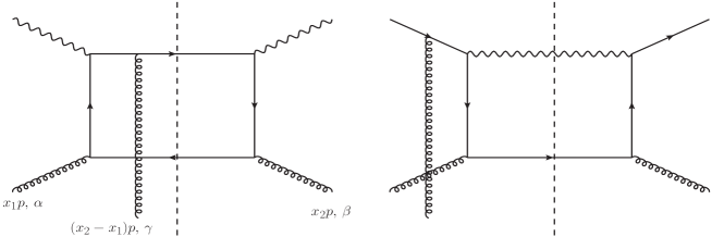
Figure 4: The diagrams which give the gluon mixing contribution to the evolution equation of $G_{q,F}(x,x)$ in SIDIS(left) and Drell-Yan(right).

The calculation technique for these diagrams was developed in Koike:2011mb . There is only the soft gluon pole($x_{1}=x_{2}$) contribution due to the interchange symmetry of the external gluon lines and then the cross section is expressed by four independent functions $O(x,x)$, $O(x,0)$, $N(x,x)$ and $N(x,0)$. The gluon mixing term in the flavor singlet evolution was discussed in both SIDIS Dai:2014ala ; Chen:2017lvx and Drell-Yan Chen:2016dnp and the cross section up to the finite term is derived as

$${d\langle P_{h\perp}\Delta\sigma\rangle^{\rm SIDIS}\over dx_{B}dydz_{h}d\phi}\Bigr{|}_{\rm gluon} \sim G_{q,F}(x_{B},x_{B},\mu)D_{q\to h}(z_{h},\mu)+{\alpha_{s}\over 2\pi}\ln\Bigl{(}{Q^{2}\over\mu^{2}}\Bigr{)}\Bigl{[}D_{q\to h}(z_{h},\mu){\cal F}_{g}\otimes T_{G+}\Bigr{]}+{\rm finite\ terms},$$

$${d\langle q_{\perp}\Delta\sigma\rangle^{\rm DY}\over dydQ^{2}}\Bigr{|}_{\rm gluon} \sim G_{q,F}(x_{a},x_{a},\mu)f_{\bar{q}/p}(x_{b},\mu)+{\alpha_{s}\over 2\pi}\ln\Bigl{(}{Q^{2}\over\mu^{2}}\Bigr{)}\Bigl{[}f_{\bar{q}/p}(x_{a},\mu){\cal F}_{g}\otimes T_{G+}\Bigl{]}+{\rm finite\ terms},$$ (60)

where $x_{a}={Q\over\sqrt{s}}e^{\eta}$, $x_{b}={Q\over\sqrt{s}}e^{-\eta}$ with the center of mass energy $\sqrt{s}$ and the rapidity $\eta$, $T_{G+}$ is given by a linear combination of the 3-gluon distribution functions and $f_{\bar{q}/p}$ is the antiquark PDF. In Drell-Yan process, we use the transverse momentum of the virtual photon $q_{\perp}$ for the weighted cross section. Using the condition as in Eq. (56), we can derive the gluon mixing term of $G_{q,F}$. The explicit form of the evolution kernel ${\cal F}_{g}$ and the finite terms are shown in Refs. Chen:2016dnp ; Chen:2017lvx . Adding the mixing term to Eq. (57), the evolution equation for the Qiu-Sterman function, the first moment of the TMD Sivers function, was completed at LO with respect to QCD coupling constant $\alpha_{s}$. As a by-product of the work on Drell-Yan, the NLO cross section related to the first momentum of the TMD Boer-Mulders function was also derived as

$${d\langle q_{\perp}\Delta\sigma\rangle^{\rm DY}\over dydQ^{2}}\Bigr{|}_{\rm BM} \sim T_{q,F}^{(\rho)}(x_{a},x_{a},\mu)h_{1}^{\bar{q}}(x_{b},\mu)+{\alpha_{s}\over 2\pi}\ln\Bigl{(}{Q^{2}\over\mu^{2}}\Bigr{)}\Bigl{[}h_{1}^{\bar{q}}(x_{a},\mu){\cal F}_{\sigma}\otimes T_{q,F}^{(\rho)}\Bigl{]}+{\rm finite\ terms},$$ (61)

where $h_{1}$ is chiral-odd transversity distribution and the twist-3 function $T_{F}^{(\rho)}(x,x,\mu)$ corresponds to the first moment of the Boer-Mulders function and its exact definition can be found in Eq. Chen:2016dnp . The evolution kernel ${\cal F}_{\sigma}$ and the finite terms of the cross section are shown in Ref. Chen:2016dnp . The authors in Ref. Chen:2017lvx also discussed the evolution equation for the first moment of the TMD Collins fragmentation function. The calculation of the twist-3 fragmentation contribution is different from the distribution case because the cross section only receives the non-pole contribution of the hard scattering. The calculation technique for the non-pole contribution has been well developed in Ref. Yuan:2009dw . It’s not difficult to extend it to the $D$-dimensional calculation. The NLO cross section was derived in Ref. Chen:2017lvx as

$${d\langle P_{h\perp}\Delta\sigma\rangle^{\rm SIDIS}\over dx_{B}dydz_{h}d\phi}\Bigr{|}_{\rm Collins} \sim h_{1}^{q}(x_{B},\mu)\hat{e}_{\partial}^{q}(z_{h},\mu)+{\alpha\over 2\pi}\ln\Bigl{(}{Q^{2}\over\mu^{2}}\Bigr{)}h_{1}^{q}(x_{B},\mu)\Bigl{[}{\cal F}_{\partial}\otimes\hat{e}^{q}_{\partial}+{\cal F}_{F}\otimes\hat{E}^{q}_{F}+{\cal F}_{G}\otimes\hat{E}^{q}_{G}\Bigr{]}$$ (62)

$$+{\rm finite\ terms},$$

where $\hat{e}_{\partial}$, $\hat{E}$ and $\hat{E}_{G}$ are the twist-3 fragmentation functions for spin-$0$ hadron(different definition is shown in Ref. Kanazawa:2015ajw ). All evolution kernels and finite terms are shown in Ref. Chen:2017lvx .

The NLO transverse-momentum-weighted cross section has been completed for single inclusive hadron production in SIDIS and Drell-Yan process in proton-proton collisions by a series of work presented here. These results are useful not only for the derivation of the evolution equations, but also for the verification of twist-3 collinear factorization feasibility, as well as for the global analysis of the experimental data. Measurement of the weighted SSAs just began very recent Alexeev:2018zvl and more data will be provided by future experiments. The analysis of the data based on the NLO result will lead to better understanding of the origin of the SSAs. There are still some TMD functions which have not been discussed yet, we hope the techniques presented in this paper can help extending the application of the transverse-momentum-weighted technique to resolve all these open questions.

The transverse-momentum-weighted technique has also been extended to study the transverse momentum broadening effect for semi-inclusive hadron production in lepton-nucleus scattering Kang:2014ela and Drell-Yan dilepton production in proton-nucleus scattering Kang:2016ron . In these studies, the QCD evolution equation for twist-4 quark-gluon correlation function was derived for the first time, and the twist-4 (double scattering) collinear factorization at NLO was confirmed through explicit calculations Kang:2013raa . The finite NLO hard parts were obtained for the transverse momentum broadening effect, which can be used in global analysis of world data to extract precisely the medium properties characterized by the twist-4 matrix elements.

V Summary

We reviewed the transverse-momentum-weighted technique as a useful tool to derive the scale evolution equation for the twist-3 collinear function which is expressed by the first moment of the TMD function. We first demonstrated the calculation of the LO cross section formula in a pedagogical way. Then we showed the basic techniques for the NLO calculation for both the virtual correction and real emission contributions. A lot of work have been done on the Qiu-Sterman function Vogelsang:2009pj ; Kang:2012ns ; Yoshida:2016tfh ; Dai:2014ala and recently the application of this technique to other twist-3 functions was also discussed Chen:2016dnp ; Chen:2017lvx . There is still room of the application to many other TMD functions by considering appropriate twist-3 observables. We hope our review paper will provide basic knowledge needed to work on this subject.

In the end, we would like to point out the importance of the $P_{h\perp}$-weighted SSA from the phenomenological point of view. We introduced this observable as a tool to derive the scale evolution equation by focusing on the ${1\over\epsilon}$-term in the cross section. However, the finite term is also important when we evaluate the cross section in order to compare it with the experimental data. The COMPASS experiment reported the data of the $P_{h\perp}$-weighted SSA very recent Alexeev:2018zvl . We expect that the data will be accumulated in the future experiments at COMPASS, JLab and EIC and then the exact NLO cross section including the finite contribution will play an important role in the analysis of those weighted SSA data.

References

• (1) R. D. Klem, J. E. Bowers, H. W. Courant, H. Kagan, M. L. Marshak, E. A. Peterson, K. Ruddick and W. H. Dragoset et al., Phys. Rev. Lett.  36, 929 (1976).
• (2) G. Bunce et al., Phys. Rev. Lett.  36, 1113 (1976).
• (3) X. d. Ji, J. p. Ma and F. Yuan, Phys. Rev.  D 71, 034005 (2005) [arXiv:hep-ph/0404183]; Phys. Lett.  B 597, 299 (2004) [arXiv:hep-ph/0405085].
• (4) S. J. Brodsky, D. S. Hwang and I. Schmidt, Phys. Lett.  B 530, 99 (2002) [arXiv:hep-ph/0201296]; Nucl. Phys.  B 642, 344 (2002) [arXiv:hep-ph/0206259].
• (5) P. J. Mulders and R. D. Tangerman, Nucl. Phys. B 461, 197 (1996) [Erratum-ibid. B 484, 538 (1997)] [arXiv:hep-ph/9510301]; A. Bacchetta, M. Diehl, K. Goeke, A. Metz, P. J. Mulders and M. Schlegel, JHEP 0702, 093 (2007) [hep-ph/0611265]; D. Boer, P. J. Mulders and F. Pijlman, Nucl. Phys.  B 667, 201 (2003) [arXiv:hep-ph/0303034].
• (6) D. Boer and P. J. Mulders, Phys. Rev. D 57, 5780 (1998) [hep-ph/9711485].
• (7) M. Anselmino, M. Boglione, U. D’Alesio, S. Melis, F. Murgia and A. Prokudin, Phys. Rev. D 79, 054010 (2009) [arXiv:0901.3078 [hep-ph]]; M. Anselmino, M. Boglione, U. D’Alesio, A. Kotzinian, S. Melis, F. Murgia, A. Prokudin and C. Turk, Eur. Phys. J. A 39, 89 (2009) [arXiv:0805.2677 [hep-ph]]; Z. -B. Kang and J. -W. Qiu, Phys. Rev. Lett.  103, 172001 (2009) [arXiv:0903.3629 [hep-ph]]; Phys. Rev. D 81, 054020 (2010) [arXiv:0912.1319 [hep-ph]]; J. C. Collins, A. V. Efremov, K. Goeke, M. Grosse Perdekamp, S. Menzel, B. Meredith, A. Metz and P. Schweitzer, Phys. Rev. D 73, 094023 (2006) [hep-ph/0511272].
• (8) A. V. Efremov and O. V. Teryaev, Sov. J. Nucl. Phys.  36, 140 (1982) [Yad. Fiz.  36, 242 (1982)]; A. V. Efremov and O. V. Teryaev, Phys. Lett. B 150, 383 (1985);
• (9) J. W. Qiu and G. Sterman, Phys. Rev. Lett.  67, 2264 (1991); Nucl. Phys.  B 378, 52 (1992); Phys. Rev.  D 59, 014004 (1999) [arXiv:hep-ph/9806356]; C. Kouvaris, J. W. Qiu, W. Vogelsang and F. Yuan, Phys. Rev.  D 74, 114013 (2006) [arXiv:hep-ph/0609238].
• (10) Y. Kanazawa and Y. Koike, Phys. Rev. D 64, 034019 (2001) [hep-ph/0012225].
• (11) H. Eguchi, Y. Koike and K. Tanaka, Nucl. Phys.  B 763, 198 (2007) [arXiv:hep-ph/0610314]; Y. Koike and K. Tanaka, Phys. Lett.  B 646, 232 (2007) [Erratum-ibid.  B 668, 458 (2008)] [arXiv:hep-ph/0612117]; Phys. Rev.  D 76, 011502 (2007) [arXiv:hep-ph/0703169]; Z. -B. Kang, F. Yuan and J. Zhou, Phys. Lett. B 691, 243 (2010) [arXiv:1002.0399 [hep-ph]]; Z. -B. Kang, A. Metz, J. -W. Qiu and J. Zhou, Phys. Rev. D 84, 034046 (2011) [arXiv:1106.3514 [hep-ph]]; L. Gamberg and Z. -B. Kang, Phys. Lett. B 718, 181 (2012) [arXiv:1208.1962 [hep-ph]].
• (12)  H. Beppu, Y. Koike, K. Tanaka and S. Yoshida, Phys. Rev. D 82, 054005 (2010) [arXiv:1007.2034 [hep-ph]]; Y. Koike and S. Yoshida, Phys. Rev. D 85, 034030 (2012) [arXiv:1112.1161 [hep-ph]]; Phys. Rev. D 84, 014026 (2011) [arXiv:1104.3943 [hep-ph]]; Z. -B. Kang and J. -W. Qiu, Phys. Rev. D 78, 034005 (2008) [arXiv:0806.1970 [hep-ph]]; Z. -B. Kang, J. -W. Qiu, W. Vogelsang and F. Yuan, Phys. Rev. D 78, 114013 (2008) [arXiv:0810.3333 [hep-ph]].
• (13) F. Yuan and J. Zhou, Phys. Rev. Lett.  103, 052001 (2009) [arXiv:0903.4680 [hep-ph]]; Z. B. Kang, F. Yuan and J. Zhou, Phys. Lett. B 691, 243 (2010) [arXiv:1002.0399 [hep-ph]]; A. Metz and D. Pitonyak, Phys. Lett. B 723, 365 (2013) [arXiv:1212.5037 [hep-ph]]; K. Kanazawa and Y. Koike, Phys. Rev. D 88, 074022 (2013) [arXiv:1309.1215 [hep-ph]].
• (14) Z. -T. Liang, A. Metz, D. Pitonyak, A. Schafer, Y. -K. Song and J. Zhou, Phys. Lett. B 712, 235 (2012) [arXiv:1203.3956 [hep-ph]]; A. Metz, D. Pitonyak, A. Schaefer and J. Zhou, arXiv:1210.6555 [hep-ph].
• (15) X. Ji, J. W. Qiu, W. Vogelsang and F. Yuan, Phys. Rev. Lett.  97, 082002 (2006) [arXiv:hep-ph/0602239]; Phys. Rev.  D 73, 094017 (2006) [arXiv:hep-ph/0604023]; Phys. Lett.  B 638, 178 (2006) [arXiv:hep-ph/0604128]; Y. Koike, W. Vogelsang and F. Yuan, Phys. Lett.  B 659, 878 (2008) [arXiv:0711.0636 [hep-ph]]; A. Bacchetta, D. Boer, M. Diehl and P. J. Mulders, JHEP 0808, 023 (2008) [arXiv:0803.0227 [hep-ph]]; D. Boer, Z. -B. Kang, W. Vogelsang and F. Yuan, Phys. Rev. Lett.  105, 202001 (2010) [arXiv:1008.3543 [hep-ph]]; Z. -B. Kang, J. -W. Qiu, W. Vogelsang and F. Yuan, Phys. Rev. D 83, 094001 (2011) [arXiv:1103.1591 [hep-ph]]; L. Gamberg and Z. -B. Kang, Phys. Lett. B 696, 109 (2011) [arXiv:1009.1936 [hep-ph]].
• (16) J. Adams et al. [STAR Collaboration], Phys. Rev. Lett.  92, 171801 (2004) [hep-ex/0310058]; B. I. Abelev et al. [STAR Collaboration], Phys. Rev. Lett.  101, 222001 (2008) [arXiv:0801.2990 [hep-ex]]; S. Heppelmann [STAR Collaboration], arXiv:0905.2840 [nucl-ex].
• (17) S. S. Adler et al. [PHENIX Collaboration], Phys. Rev. Lett.  95, 202001 (2005) [hep-ex/0507073].
• (18) I. Arsene et al. [BRAHMS Collaboration], Phys. Rev. Lett.  101, 042001 (2008) [arXiv:0801.1078 [nucl-ex]].
• (19) K. Kanazawa, Y. Koike, A. Metz and D. Pitonyak, Phys. Rev. D 89, no. 11, 111501 (2014) [arXiv:1404.1033 [hep-ph]].
• (20) L. Gamberg, Z. B. Kang, D. Pitonyak and A. Prokudin, Phys. Lett. B 770, 242 (2017) [arXiv:1701.09170 [hep-ph]].
• (21) Z. B. Kang and J. W. Qiu, Phys. Rev. D 79, 016003 (2009) [arXiv:0811.3101 [hep-ph]].
• (22) J. Zhou, F. Yuan and Z. T. Liang, Phys. Rev. D 79, 114022 (2009) [arXiv:0812.4484 [hep-ph]].
• (23) V. M. Braun, A. N. Manashov and B. Pirnay, Phys. Rev. D 80, 114002 (2009) Erratum: [Phys. Rev. D 86, 119902 (2012)] [arXiv:0909.3410 [hep-ph]].
• (24) A. Schafer and J. Zhou, Phys. Rev. D 85, 117501 (2012) [arXiv:1203.5293 [hep-ph]].
• (25) J. P. Ma and Q. Wang, Phys. Lett. B 715, 157 (2012) [arXiv:1205.0611 [hep-ph]].
• (26) Z. B. Kang and J. W. Qiu, Phys. Lett. B 713, 273 (2012) [arXiv:1205.1019 [hep-ph]].
• (27) Z. B. Kang, Phys. Rev. D 83, 036006 (2011) [arXiv:1012.3419 [hep-ph]].
• (28) J. P. Ma and G. P. Zhang, Phys. Lett. B 772, 559 (2017) [arXiv:1701.04141 [hep-ph]].
• (29) W. Vogelsang and F. Yuan, Phys. Rev. D 79, 094010 (2009) [arXiv:0904.0410 [hep-ph]].
• (30) Z. B. Kang, I. Vitev and H. Xing, Phys. Rev. D 87, no. 3, 034024 (2013) [arXiv:1212.1221 [hep-ph]].
• (31) S. Yoshida, Phys. Rev. D 93, no. 5, 054048 (2016) [arXiv:1601.07737 [hep-ph]].
• (32) L. Y. Dai, Z. B. Kang, A. Prokudin and I. Vitev, Phys. Rev. D 92, no. 11, 114024 (2015) [arXiv:1409.5851 [hep-ph]].
• (33) A. P. Chen, J. P. Ma and G. P. Zhang, Phys. Rev. D 95, no. 7, 074005 (2017) [arXiv:1607.08676 [hep-ph]].
• (34) A. P. Chen, J. P. Ma and G. P. Zhang, Phys. Rev. D 97, no. 5, 054003 (2018) [arXiv:1708.09091 [hep-ph]].
• (35) M. G. Alexeev et al. [COMPASS Collaboration], arXiv:1809.02936 [hep-ex].
• (36) Y. Koike and K. Tanaka, Phys. Lett. B 646, 232 (2007) Erratum: [Phys. Lett. B 668, 458 (2008)] [hep-ph/0612117].
• (37) K. Kanazawa, Y. Koike, A. Metz, D. Pitonyak and M. Schlegel, Phys. Rev. D 93, no. 5, 054024 (2016) [arXiv:1512.07233 [hep-ph]].
• (38) Z. B. Kang, E. Wang, X. N. Wang and H. Xing, Phys. Rev. D 94, no. 11, 114024 (2016) doi:10.1103/PhysRevD.94.114024 [arXiv:1409.1315 [hep-ph]].
• (39) Z. B. Kang, J. W. Qiu, X. N. Wang and H. Xing, Phys. Rev. D 94, no. 7, 074038 (2016) doi:10.1103/PhysRevD.94.074038 [arXiv:1605.07175 [hep-ph]].
• (40) Z. B. Kang, E. Wang, X. N. Wang and H. Xing, Phys. Rev. Lett.  112, no. 10, 102001 (2014) doi:10.1103/PhysRevLett.112.102001 [arXiv:1310.6759 [hep-ph]].