IFT-UAM/CSIC-19-020
LAPTH-004/19
Reduction of Couplings and its application
in Particle Physics

Abstract

The idea of reduction of couplings in renormalizable theories will be presented and then will be applied in Particle Physics models. Reduced couplings appeared as functions of a primary one, compatible with the renormalization group equation and thus solutions of a specific set of ordinary differential equations. If these functions have the form of power series the respective theories resemble standard renormalizable ones and thus widen considerably the area covered until then by symmetries as a tool for constraining the number of couplings consistently. Still on the more abstract level reducing couplings enabled one to construct theories with beta-functions vanishing to all orders of perturbation theory. Reduction of couplings became physics-wise truly interesting and phenomenologically important when applied to the standard model and its possible extensions. In particular in the context of supersymmetric theories it became the most powerful tool known today once it was learned how to apply it also to couplings having dimension of mass and to mass parameters. Technically this all relies on the basic property that reducing couplings is a renormalization scheme independent procedure. Predictions of top and Higgs mass prior to their experimental finding highlight the fundamental physical significance of this notion.

Prologue and Synopsis

In spite of their limitations, perturbative local field theories are still of prominent practical value.

It is remarkable that the intrinsic ambiguities connected with locality and causality - most of the time associated with ultraviolet infinities - can be summarized in terms of a formal group which acts in the space of the coupling constants or coupling functions attached to each type of local interaction.

It is therefore natural to look systematically for stable submanifolds. Some such have been known for a long time: e.g., spaces of renormalizable interactions and subspaces characterized by system of Ward identities mostly related to symmetries.

A systematic search for such stable submanifolds has been initiated by W. Zimmermann in the early eighties.

Disappointing for some time, this program has attracted several other active researchers and recently produced physically interesting results.

It looks at the moment as the only theoretically founded algorithm potentially able to decrease the number of parameters within the physically favoured perturbative models .

Raymond Stora, CERN (Switzerland), December 16, 2013

Chapter 1 Introduction: The Basic Ideas

In the recent years the theoretical endeavours that attempt to achieve a deeper understanding of Nature have presented a series of successes in developing frameworks such as String Theories and Noncommutativity that aim to describe the fundamental theory at the Planck scale. However, the essence of all theoretical efforts in Elementary Particle Physics (EPP) is to understand the present day free parameters of the Standard Model (SM) in terms of few fundamental ones, i.e. to achieve reductions of couplings[1]. Unfortunately, despite the several successes in the above frameworks they do not offer anything in the understanding of the free paramaters of the SM. The pathology of the plethora of free parameters is deeply connected to the presence of infinities at the quantum level. The renormalization program can remove the infinities by introducing counterterms, but only at the cost of leaving the corresponding terms as free parameters.

Although the Standard Model (SM) has been very successful in describing elementary particles and its interactions, it has been known for some time that it must be the low energy limit of a more fundamental theory. This quest for a theory beyond the Standard Model (BSM) has expanded in various directions. The usual, and very efficient, way of reducing the number of free parameters of a theory to render it more predictive, is to introduce a symmetry. Grand Unified Theories (GUTs) are very good examples of such a procedure [2, 3, 4, 5, 6, 7]. First in the case of minimal $SU(5)$, because of the (approximate) gauge coupling unification, it was possible to reduce the gauge couplings of the SM and give a prediction for one of them. By adding a further symmetry, namely $N=1$ global supersymmetry [8, 9, 10] it was possible to make the prediction viable. GUTs can also relate the Yukawa couplings among themselves, again $SU(5)$ provided an example of this by predicting the ratio $M_{\tau}/M_{b}$ [11] in the SM. Unfortunately, requiring more gauge symmetry does not seem to help, since additional complications are introduced due to new degrees of freedom, for instance in the ways and channels of breaking the symmetry.

A possible way to look for relations among unrelated parameters is the method of reduction of couplings [12, 13, 14]; see also refs [15, 16, 17]. This method, as its name proclaims, reduces the number of couplings in a theory by relating either all or a number of couplings to a single coupling denoted as the “primary coupling”. This method might help to identify hidden symmetries in a system, but it is also possible to have reduction of couplings in systems where there is no apparent symmetry. The reduction of couplings is based on the assumption that both the original and the reduced theory are renormalizable and that there exist renormalization group invariant (RGI) relations among parameters.

A natural extension of the GUT idea and successful application of the method of reduction of couplings is to find a way to relate the gauge and Yukawa sectors of a theory, that is to achieve gauge-Yukawa Unification (GYU). This will be presented in Chapter 5. Following the original suggestion for reducing the couplings within the framework of GUTs we were hunting for renormalization group invariant (RGI) relations holding below the Planck scale, which in turn are preserved down to the GUT scale. It is indeed an impressive observation that one can guarantee the validity of the RGI relations to all-orders in perturbation theory by studying the uniqueness of the resulting relations at one-loop. Even more remarkable is the fact that it is possible to find RGI relations among couplings that guarantee finiteness to all-orders in perturbation theory. The above principles have only been applied in $N=1$ supersymmetric GUTs for reasons that will be transparent in the following sections, here we should only note that the use of $N=1$ supersymmetric GUTs comprises the demand of the cancellation of quadratic divergencies in the SM. The above GYU program applied in the dimensionless couplings of supersymmetric GUTs had a great success by predicting correctly, among others, the top quark mass in the finite [18, 19] and in the minimal $N=1$ supersymmetric $SU(5)$ [20] before its discovery [21].

Although supersymmetry seems to be an essential feature for a successful realization of the above program, its breaking has to be understood too, since it has the ambition to supply the SM with predictions for several of its free parameters. Indeed, the search for RGI relations has been extended to the soft supersymmetry breaking sector (SSB) of these theories, which involves parameters of dimension one and two. In addition, there was important progress concerning the renormalization properties of the SSB parameters, based on the powerful supergraph method for studying supersymmetric theories, and it was applied to the softly broken ones by using the “spurion” external space-time independent superfields. According to this method a softly broken supersymmetric gauge theory is considered as a supersymmetric one in which the various parameters, such as couplings and masses, have been promoted to external superfields. Then, relations among the soft term renormalization and that of an unbroken supersymmetric theory have been derived. In particular the $\beta$-functions of the parameters of the softly broken theory are expressed in terms of partial differential operators involving the dimensionless parameters of the unbroken theory. The key point in solving the set of coupled differential equations so as to be able to express all parameters in a RGI way, was to transform the partial differential operators involved to total derivative operators. It is indeed possible to do this by choosing a suitable RGI surface.

On the phenomenological side the application on the reduction of coupling method to $N=1$ supersymmetric theories has led to very interesting developments too. Previously an appealing “universal” set of soft scalar masses was assumed in the SSB sector of supersymmetric theories, given that apart from economy and simplicity (1) they are part of the constraints that preserve finiteness up to two-loops, (2) they appear in the attractive dilaton dominated supersymmetry breaking superstring scenarios. However, further studies have exhibited a number of problems, all due to the restrictive nature of the “universality” assumption for the soft scalar masses. Therefore, there were attempts to relax this constraint without loosing its attractive features. Indeed an interesting observation on $N=1$ GYU theories is that there exists a RGI sum rule for the soft scalar masses at lower orders in perturbation theory, which was later extended to all-orders, and manages to overcome all the unpleasant phenomenological consequences. Armed with the above tools and results we were in a position to study the spectrum of the full finite models in terms of few free parameters, with emphasis on the predictions of supersymmetric particles and the lightest Higgs mass.

The result was indeed very impressive since it led to a prediction of the Higgs mass which coincided with the results of the LHC for the Higgs mass by ATLAS [22, 23] and CMS [24, 25], and predicted a relatively heavy spectrum consistent with the non-observation of supersymmetric particles at the LHC. The coloured supersymmetric particles are predicted to be above 2.7 TeV, while the electroweak supersymmetric spectrum starts below 1 TeV. These successes will be presented in Chapter 6.

Last but certainly not least, the above machinery has been recently applied in the MSSM with impressive results concerning the predictivity of the top, bottom and Higgs masses, being at the same time consistent with the non-observation of supersymmeric particles at the LHC. More specifically the electroweak supersymmetric spectrum starts at 1.3 TeV and the coloured at $\sim 4$ TeV. These results will be presented too in Chapter 6.

Chapter 2 Theoretical Basis

2.1 Reduction of Dimensionless Parameters

In this section we outline the idea of reduction of couplings. Any RGI relation among couplings (i.e. which does not depend on the renormalization scale $\mu$ explicitly) can be expressed, in the implicit form $\Phi(g_{1},\cdots,g_{A})~{}=~{}\mbox{const.}$, which has to satisfy the partial differential equation (PDE)

$$\mu\,\frac{d\Phi}{d\mu}={\vec{\nabla}}\Phi\cdot{\vec{\beta}}~{}=~{}\sum_{a=1}^{A}\,\beta_{a}\,\frac{\partial\Phi}{\partial g_{a}}~{}=~{}0~{},$$ (2.1)

where $\beta_{a}$ is the $\beta$-function of $g_{a}$. This PDE is equivalent to a set of ordinary differential equations, the so-called reduction equations (REs) [12, 13, 14],

$$\beta_{g}\,\frac{dg_{a}}{dg}=\beta_{a}~{},~{}a=1,\cdots,A~{},$$ (2.2)

where $g$ and $\beta_{g}$ are the primary coupling and its $\beta$-function, and the counting on $a$ does not include $g$. Since maximally ($A-1$) independent RGI “constraints” in the $A$-dimensional space of couplings can be imposed by the $\Phi_{a}$’s, one could in principle express all the couplings in terms of a single coupling $g$. However, a closer look to the set of Eqs. (2.2) reveals that their general solutions contain as many integration constants as the number of equations themselves. Thus, using such integration constants we have just traded an integration constant for each ordinary renormalized coupling, and consequently, these general solutions cannot be considered as reduced ones. The crucial requirement in the search for RGE relations is to demand power series solutions to the REs,

$$g_{a}=\sum_{n}\rho_{a}^{(n)}\,g^{2n+1}~{},$$ (2.3)

which preserve perturbative renormalizability. Such an ansatz fixes the corresponding integration constant in each of the REs and picks up a special solution out of the general one. Remarkably, the uniqueness of such power series solutions can be decided already at the one-loop level [12, 13, 14]. To illustrate this, let us assume that the $\beta$-functions have the form

$$\begin{split}\beta_{a}&=\frac{1}{16\pi^{2}}\left[\sum_{b,c,d\neq g}\beta^{(1)\,bcd}_{a}g_{b}g_{c}g_{d}+\sum_{b\neq g}\beta^{(1)\,b}_{a}g_{b}g^{2}\right]+\cdots~{},\\ \beta_{g}&=\frac{1}{16\pi^{2}}\beta^{(1)}_{g}g^{3}+\cdots~{},\end{split}$$ (2.4)

where $\cdots$ stands for higher order terms, and $\beta^{(1)\,bcd}_{a}$’s are symmetric in $b,c,d$. We then assume that the $\rho_{a}^{(n)}$’s with $n\leq r$ have been uniquely determined. To obtain $\rho_{a}^{(r+1)}$’s, we insert the power series (2.3) into the REs (2.2) and collect terms of ${\cal O}(g^{2r+3})$ and find

$$\sum_{d\neq g}M(r)_{a}^{d}\,\rho_{d}^{(r+1)}=\mbox{lower order quantities}~{},$$

where the r.h.s. is known by assumption, and

$$M(r)_{a}^{d} =3\sum_{b,c\neq g}\,\beta^{(1)\,bcd}_{a}\,\rho_{b}^{(1)}\,\rho_{c}^{(1)}+\beta^{(1)\,d}_{a}-(2r+1)\,\beta^{(1)}_{g}\,\delta_{a}^{d}~{},$$ (2.5)

$$0 =\sum_{b,c,d\neq g}\,\beta^{(1)\,bcd}_{a}\,\rho_{b}^{(1)}\,\rho_{c}^{(1)}\,\rho_{d}^{(1)}+\sum_{d\neq g}\beta^{(1)\,d}_{a}\,\rho_{d}^{(1)}-\beta^{(1)}_{g}\,\rho_{a}^{(1)}~{}.$$ (2.6)

Therefore, the $\rho_{a}^{(n)}$’s for all $n>1$ for a given set of $\rho_{a}^{(1)}$’s can be uniquely determined if $\det M(n)_{a}^{d}\neq 0$ for all $n\geq 0$.

As it will be clear later by examining specific examples, the various couplings in supersymmetric theories have the same asymptotic behaviour. Therefore searching for a power series solution of the form (2.3) to the REs (2.2) is justified.

The possibility of coupling unification described in this section is without any doubt attractive because the “completely reduced” theory contains only one independent coupling, but it can be unrealistic. Therefore, one often would like to impose fewer RGI constraints, and this is the idea of partial reduction [26, 27].

The above facts lead us to suspect that there is and intimate connection among the requirement of reduction of couplings and supersymmetry which still waits to be uncovered. The connection becomes more clear by examining the following example.

Consider an $SU(N)$ gauge theory with the following matter content: $\phi^{i}({\bf N})$ and $\hat{\phi}_{i}(\overline{\bf N})$ are complex scalars, $\psi^{i}({\bf N})$ and $\hat{\psi}_{i}(\overline{\bf N})$ are left-handed Weyl spinor, and $\lambda^{a}(a=1,\dots,N^{2}-1)$ is a right-handed Weyl spinor in the adjoint representation of $SU(N)$.

The Lagrangian, omitting kinetic terms, includes:

$${\cal L}\supset i\sqrt{2}\{~{}g_{Y}\overline{\psi}\lambda^{a}T^{a}\phi-\hat{g}_{Y}\overline{\hat{\psi}}\lambda^{a}T^{a}\hat{\phi}+\mbox{h.c.}~{}\}-V(\phi,\overline{\phi}),$$ (2.7)

where

$$V(\phi,\overline{\phi})=\frac{1}{4}\lambda_{1}(\phi^{i}\phi^{*}_{i})^{2}+\frac{1}{4}\lambda_{2}(\hat{\phi}_{i}\hat{\phi}^{*~{}i})^{2}+\lambda_{3}(\phi^{i}\phi^{*}_{i})(\hat{\phi}_{j}\hat{\phi}^{*~{}j})+\lambda_{4}(\phi^{i}\phi^{*}_{j})(\hat{\phi}_{i}\hat{\phi}^{*~{}j}),$$ (2.8)

which is the most general renormalizable form of dimension four, consistent with the $SU(N)\times SU(N)$ global symmetry.

Searching for a solution of the form of Eq. (2.3) for the REs (2.2,) we find in lowest order the following one ($g$ is the gauge coupling):

$$\begin{split}g_{Y}&=\hat{g}_{Y}=g~{},\\ \lambda_{1}&=\lambda_{2}=\frac{N-1}{N}g^{2}~{},\\ \lambda_{3}&=\frac{1}{2N}g^{2}~{},~{}\lambda_{4}=-\frac{1}{2}g^{2}~{},\end{split}$$ (2.9)

which corresponds to an $N=1$ supersymmetric gauge theory. Clearly the above remarks do not answer the question of the relation among reduction of couplings and supersymmetry but rather try to trigger the interest for further investigation.

2.2 Reduction of Couplings in N = 1 Supersymmetric Gauge Theories. Partial Reduction

Let us consider a chiral, anomaly free, $N=1$ globally supersymmetric gauge theory based on a group G with gauge coupling constant $g$. The superpotential of the theory is given by

$$W = \frac{1}{2}\,m_{ij}\,\phi_{i}\,\phi_{j}+\frac{1}{6}\,C_{ijk}\,\phi_{i}\,\phi_{j}\,\phi_{k}~{},$$ (2.10)

where $m_{ij}$ and $C_{ijk}$ are gauge invariant tensors and the matter field (chiral superfield) $\phi_{i}$ transforms according to the irreducible representation $R_{i}$ of the gauge group $G$. The renormalization constants associated with the superpotential (2.10), assuming that supersymmetry is preserved, are

$$\phi_{i}^{0} =\left(Z^{j}_{i}\right)^{(1/2)}\,\phi_{j}~{},~{}$$ (2.11)

$$m_{ij}^{0} =Z^{i^{\prime}j^{\prime}}_{ij}\,m_{i^{\prime}j^{\prime}}~{},~{}$$ (2.12)

$$C_{ijk}^{0} =Z^{i^{\prime}j^{\prime}k^{\prime}}_{ijk}\,C_{i^{\prime}j^{\prime}k^{\prime}}~{}.$$ (2.13)

The $N=1$ non-renormalization theorem [28, 29, 30, 31] ensures that there are no mass and cubic-interaction-term infinities and therefore

$$\begin{split}Z_{ij}^{i^{\prime}j^{\prime}}\left(Z^{i^{\prime\prime}}_{i^{\prime}}\right)^{(1/2)}\left(Z^{j^{\prime\prime}}_{j^{\prime}}\right)^{(1/2)}&=\delta_{(i}^{i^{\prime\prime}}\,\delta_{j)}^{j^{\prime\prime}}~{},\\ Z_{ijk}^{i^{\prime}j^{\prime}k^{\prime}}\left(Z^{i^{\prime\prime}}_{i^{\prime}}\right)^{(1/2)}\left(Z^{j^{\prime\prime}}_{j^{\prime}}\right)^{(1/2)}\left(Z^{k^{\prime\prime}}_{k^{\prime}}\right)^{(1/2)}&=\delta_{(i}^{i^{\prime\prime}}\,\delta_{j}^{j^{\prime\prime}}\delta_{k)}^{k^{\prime\prime}}~{}.\end{split}$$ (2.14)

As a result the only surviving possible infinities are the wave-function renormalization constants $Z^{j}_{i}$, i.e., one infinity for each field. The one-loop $\beta$-function of the gauge coupling $g$ is given by [32, 33, 34, 35, 36]

$$\beta^{(1)}_{g}=\frac{dg}{dt}=\frac{g^{3}}{16\pi^{2}}\left[\,\sum_{i}\,T(R_{i})-3\,C_{2}(G)\right]~{},$$ (2.15)

where, as usual, $t$ is the logarithm of the ratio of the energy scale over a reference scale, $C_{2}(G)$ is the quadratic Casimir of the adjoint representation of the associated gauge group $G$ and $T(R)$ is given by the relation $\textrm{Tr}[T^{a}T^{b}]=T(R)\delta^{ab}$ while $T^{a}$ is the generators of the group in the appropriate representation. The $\beta$-functions of $C_{ijk}$, by virtue of the non-renormalization theorem, are related to the anomalous dimension matrix $\gamma_{ij}$ of the matter fields $\phi_{i}$ as:

$$\beta_{ijk}=\frac{dC_{ijk}}{dt}~{}=~{}C_{ijl}\,\gamma^{l}_{k}+C_{ikl}\,\gamma^{l}_{j}+C_{jkl}\,\gamma^{l}_{i}~{}.$$ (2.16)

At one-loop level $\gamma^{i}_{j}$ is given by [32]

$$\gamma^{(1)}{}_{j}^{i}=\frac{1}{32\pi^{2}}\,[\,C^{ikl}\,C_{jkl}-2\,g^{2}\,C_{2}(R_{i})\delta^{i}_{j}\,],$$ (2.17)

where $C_{2}(R_{i})$ is the quadratic Casimir of the representation $R_{i}$, and $C^{ijk}=C_{ijk}^{*}$. Since dimensional coupling parameters such as masses and couplings of scalar field cubic terms do not influence the asymptotic properties of a theory on which we are interested here, it is sufficient to take into account only the dimensionless supersymmetric couplings such as $g$ and $C_{ijk}$. So we neglect the existence of dimensional parameters, and assume furthermore that $C_{ijk}$ are real so that $C_{ijk}^{2}$ always are positive numbers. For our purposes, it is convenient to work with the square of the couplings and to arrange $C_{ijk}$ in such a way that they are covered by a single index $i~{}(i=1,\cdots,n)$:

$$\alpha=\frac{g^{2}}{4\pi}~{},~{}\alpha_{i}~{}=~{}\frac{g_{i}^{2}}{4\pi}~{}.$$ (2.18)

The evolution equations of $\alpha$’s in perturbation theory then take the form

$$\begin{split}\frac{d\alpha}{dt}&=\beta~{}=~{}-\beta^{(1)}\alpha^{2}+\cdots~{},\\ \frac{d\alpha_{i}}{dt}&=\beta_{i}~{}=~{}-\beta^{(1)}_{i}\,\alpha_{i}\,\alpha+\sum_{j,k}\,\beta^{(1)}_{i,jk}\,\alpha_{j}\,\alpha_{k}+\cdots~{},\end{split}$$ (2.19)

where $\cdots$ denotes the contributions from higher orders, and $\beta^{(1)}_{i,jk}=\beta^{(1)}_{i,kj}$.

Given the set of the evolution equations (2.19), we investigate the asymptotic properties, as follows. First we define [12, 14, 37, 38, 16]

$$\tilde{\alpha}_{i}\equiv\frac{\alpha_{i}}{\alpha}~{},~{}i=1,\cdots,n~{},$$ (2.20)

and derive from Eq. (2.19)

$$\begin{split}\alpha\frac{d\tilde{\alpha}_{i}}{d\alpha}&=-\tilde{\alpha}_{i}+\frac{\beta_{i}}{\beta}=\left(-1+\frac{\beta^{(1)}_{i}}{\beta^{(1)}}\,\right)\tilde{\alpha}_{i}\\ &-\sum_{j,k}\,\frac{\beta^{(1)}_{i,jk}}{\beta^{(1)}}\,\tilde{\alpha}_{j}\,\tilde{\alpha}_{k}+\sum_{r=2}\,\left(\frac{\alpha}{\pi}\right)^{r-1}\,\tilde{\beta}^{(r)}_{i}(\tilde{\alpha})~{},\end{split}$$ (2.21)

where $\tilde{\beta}^{(r)}_{i}(\tilde{\alpha})~{}(r=2,\cdots)$ are power series of $\tilde{\alpha}$’s and can be computed from the $r$-th loop $\beta$-functions. Next we search for fixed points $\rho_{i}$ of Eq. (2.20) at $\alpha=0$. To this end, we have to solve

$$\left(-1+\frac{\beta^{(1)}_{i}}{\beta^{(1)}}\right)\rho_{i}-\sum_{j,k}\frac{\beta^{(1)}_{i,jk}}{\beta^{(1)}}\,\rho_{j}\,\rho_{k}=0~{},$$ (2.22)

and assume that the fixed points have the form

$$\rho_{i}=0~{}\mbox{for}~{}i=1,\cdots,n^{\prime}~{};~{}\rho_{i}~{}>0~{}\mbox{for}~{}i=n^{\prime}+1,\cdots,n~{}.$$ (2.23)

We then regard $\tilde{\alpha}_{i}$ with $i\leq n^{\prime}$ as small perturbations to the undisturbed system which is defined by setting $\tilde{\alpha}_{i}$ with $i\leq n^{\prime}$ equal to zero. As we have seen, it is possible to verify at the one-loop level [12, 13, 14, 37] the existence of the unique power series solution

$$\tilde{\alpha}_{i}=\rho_{i}+\sum_{r=2}\rho^{(r)}_{i}\,\alpha^{r-1}~{},~{}i=n^{\prime}+1,\cdots,n~{}$$ (2.24)

of the reduction equations (2.21) to all orders in the undisturbed system. These are RGI relations among couplings and keep formally perturbative renormalizability of the undisturbed system. So in the undisturbed system there is only one independent coupling, the primary coupling $\alpha$.

The small perturbations caused by nonvanishing $\tilde{\alpha}_{i}$ with $i\leq n^{\prime}$ enter in such a way that the reduced couplings, i.e. $\tilde{\alpha}_{i}$ with $i>n^{\prime}$, become functions not only of $\alpha$ but also of $\tilde{\alpha}_{i}$ with $i\leq n^{\prime}$. It turned out that, to investigate such partially reduced systems, it is most convenient to work with the partial differential equations

$$\begin{split}\left\{\tilde{\beta}\,\frac{\partial}{\partial\alpha}+\sum_{a=1}^{n^{\prime}}\,\tilde{\beta_{a}}\,\frac{\partial}{\partial\tilde{\alpha}_{a}}\right\}~{}\tilde{\alpha}_{i}(\alpha,\tilde{\alpha})&=\tilde{\beta}_{i}(\alpha,\tilde{\alpha})~{},\\ \tilde{\beta}_{i(a)}~{}=~{}\frac{\beta_{i(a)}}{\alpha^{2}}-\frac{\beta}{\alpha^{2}}~{}\tilde{\alpha}_{i(a)}&,\qquad\tilde{\beta}~{}\equiv~{}\frac{\beta}{\alpha}~{},\end{split}$$ (2.25)

which are equivalent to the reduction equations (2.21), where we let $a,b$ run from $1$ to $n^{\prime}$ and $i,j$ from $n^{\prime}+1$ to $n$ in order to avoid confusion. We then look for solutions of the form

$$\tilde{\alpha}_{i}=\rho_{i}+\sum_{r=2}\,\left(\frac{\alpha}{\pi}\right)^{r-1}\,f^{(r)}_{i}(\tilde{\alpha}_{a})~{},~{}i=n^{\prime}+1,\cdots,n~{},$$ (2.26)

where $f^{(r)}_{i}(\tilde{\alpha}_{a})$ are supposed to be power series of $\tilde{\alpha}_{a}$. This particular type of solution can be motivated by requiring that in the limit of vanishing perturbations we obtain the undisturbed solutions (2.24) [27, 39]. Again it is possible to obtain the sufficient conditions for the uniqueness of $f^{(r)}_{i}$ in terms of the lowest order coefficients.

2.3 Reduction of Dimension-1 and -2 Parameters

The reduction of couplings was originally formulated for massless theories on the basis of the Callan-Symanzik equation [12, 13]. The extension to theories with massive parameters is not straightforward if one wants to keep the generality and the rigor on the same level as for the massless case; one has to fulfill a set of requirements coming from the renormalization group equations, the Callan-Symanzik equations, etc. along with the normalization conditions imposed on irreducible Green’s functions [40]. There has been a lot of progress in this direction starting from ref. [41], as it is already mentioned in the Introduction, where it was assumed that a mass-independent renormalization scheme could be employed so that all the RG functions have only trivial dependencies on dimensional parameters and then the mass parameters were introduced similarly to couplings (i.e. as a power series in the couplings). This choice was justified later in [42, 43] where the scheme independence of the reduction principle has been proven generally, i.e it was shown that apart from dimensionless couplings, pole masses and gauge parameters, the model may also involve coupling parameters carrying a dimension and masses. Therefore here, to simplify the analysis, we follow Ref. [41] and make use also of a mass-independent renormalization scheme.

We start by considering a renormalizable theory which contain a set of $(N+1)$ dimension-zero couplings, $\left(\hat{g}_{0},\hat{g}_{1},...,\hat{g}_{N}\right)$, a set of $L$ parameters with mass-dimension one, $\left(\hat{h}_{1},...,\hat{h}_{L}\right)$, and a set of $M$ parameters with mass-dimension two, $\left(\hat{m}_{1}^{2},...,\hat{m}_{M}^{2}\right)$. The renormalized irreducible vertex function $\Gamma$ satisfies the RG equation

$$\mathcal{D}\Gamma\left[\Phi^{\prime}s;\hat{g}_{0},\hat{g}_{1},...,\hat{g}_{N};\hat{h}_{1},...,\hat{h}_{L};\hat{m}_{1}^{2},...,\hat{m}_{M}^{2};\mu\right]=0~{},$$ (2.27)

where

$$\mathcal{D}=\mu\frac{\partial}{\partial\mu}+\sum_{i=0}^{N}\beta_{i}\frac{\partial}{\partial\hat{g}_{i}}+\sum_{a=1}^{L}\gamma_{a}^{h}\frac{\partial}{\partial\hat{h}_{a}}+\sum_{\alpha=1}^{M}\gamma_{\alpha}^{m^{2}}\frac{\partial}{\partial\hat{m}_{\alpha}^{2}}+\sum_{J}\Phi_{I}\gamma^{\phi I}_{\,\,\,\,J}\,\frac{\delta}{\delta\Phi_{J}}~{},$$ (2.28)

where $\mu$ is the energy scale, while $\beta_{i}$ are the $\beta$-functions of the various dimensionless couplings $g_{i}$, $\Phi_{I}$ are the various matter fields and $\gamma_{\alpha}^{m^{2}}$, $\gamma_{a}^{h}$ and $\gamma^{\phi I}_{\,\,\,\,J}$ are the mass, trilinear coupling and wave function anomalous dimensions, respectively (where $I$ enumerates the matter fields). In a mass independent renormalization scheme, the $\gamma$’s are given by

$$\begin{split}\gamma^{h}_{a}&=\sum_{b=1}^{L}\gamma_{a}^{h,b}(g_{0},g_{1},...,g_{N})\hat{h}_{b},\\ \gamma_{\alpha}^{m^{2}}&=\sum_{\beta=1}^{M}\gamma_{\alpha}^{m^{2},\beta}(g_{0},g_{1},...,g_{N})\hat{m}_{\beta}^{2}+\sum_{a,b=1}^{L}\gamma_{\alpha}^{m^{2},ab}(g_{0},g_{1},...,g_{N})\hat{h}_{a}\hat{h}_{b},\end{split}$$ (2.29)

where $\gamma_{a}^{h,b}$, $\gamma_{\alpha}^{m^{2},\beta}$ and $\gamma_{\alpha}^{m^{2},ab}$ are power series of the $g$’s (which are dimensionless) in perturbation theory.

We look for a reduced theory where

$$g\equiv g_{0},\qquad h_{a}\equiv\hat{h}_{a}\quad\textrm{for $1\leq a\leq P$},\qquad m^{2}_{\alpha}\equiv\hat{m}^{2}_{\alpha}\quad\textrm{for $1\leq\alpha\leq Q$}$$

are independent parameters and the reduction of the remaining parameters

$$\begin{split}\hat{g}_{i}&=\hat{g}_{i}(g),\qquad(i=1,...,N),\\ \hat{h}_{a}&=\sum_{b=1}^{P}f_{a}^{b}(g)h_{b},\qquad(a=P+1,...,L),\\ \hat{m}^{2}_{\alpha}&=\sum_{\beta=1}^{Q}e^{\beta}_{\alpha}(g)m^{2}_{\beta}+\sum_{a,b=1}^{P}k^{ab}_{\alpha}(g)h_{a}h_{b},\qquad(\alpha=Q+1,...,M)\end{split}$$ (2.30)

is consistent with the RG equations (2.27,2.28). It turns out that the following relations should be satisfied

$$\begin{split}\beta_{g}\,\frac{\partial\hat{g}_{i}}{\partial g}&=\beta_{i},\qquad(i=1,...,N),\\ \beta_{g}\,\frac{\partial\hat{h}_{a}}{\partial g}+\sum_{b=1}^{P}\gamma^{h}_{b}\,\frac{\partial\hat{h}_{a}}{\partial h_{b}}&=\gamma^{h}_{a},\qquad(a=P+1,...,L),\\ \beta_{g}\,\frac{\partial\hat{m}^{2}_{\alpha}}{\partial g}+\sum_{a=1}^{P}\gamma_{a}^{h}\,\frac{\partial\hat{m}^{2}_{\alpha}}{\partial h_{a}}+\sum_{\beta=1}^{Q}\gamma_{\beta}^{m^{2}}\,\frac{\partial\hat{m}_{\alpha}^{2}}{\partial m_{\beta}^{2}}&=\gamma_{\alpha}^{m^{2}},\qquad(\alpha=Q+1,...,M).\end{split}$$ (2.31)

Using Eqs. (2.29) and (2.30), the above relations reduce to

$$\begin{split}&\beta_{g}\,\frac{df^{b}_{a}}{dg}+\sum_{c=1}^{P}f^{c}_{a}\left[\gamma^{h,b}_{c}+\sum_{d=P+1}^{L}\gamma^{h,d}_{c}f^{b}_{d}\right]-\gamma^{h,b}_{a}-\sum_{d=P+1}^{L}\gamma^{h,d}_{a}f^{b}_{d}=0,\\ &\hskip 244.69386pt(a=P+1,...,L;\,b=1,...,P),\\ &\beta_{g}\,\frac{de^{\beta}_{\alpha}}{dg}+\sum_{\gamma=1}^{Q}e^{\gamma}_{\alpha}\left[\gamma_{\gamma}^{m^{2},\beta}+\sum_{\delta=Q+1}^{M}\gamma_{\gamma}^{m^{2},\delta}e^{\beta}_{\delta}\right]-\gamma_{\alpha}^{m^{2},\beta}-\sum_{\delta=Q+1}^{M}\gamma_{\alpha}^{m^{2},d}e^{\beta}_{\delta}=0,\\ &\hskip 236.15796pt(\alpha=Q+1,...,M;\,\beta=1,...,Q),\\ &\beta_{g}\,\frac{dk_{\alpha}^{ab}}{dg}+2\sum_{c=1}^{P}\left(\gamma_{c}^{h,a}+\sum_{d=P+1}^{L}\gamma_{c}^{h,d}f_{d}^{a}\right)k_{\alpha}^{cb}+\sum_{\beta=1}^{Q}e^{\beta}_{\alpha}\left[\gamma_{\beta}^{m^{2},ab}+\sum_{c,d=P+1}^{L}\gamma_{\beta}^{m^{2},cd}f^{a}_{c}f^{b}_{d}\right.\\ &\left.+2\sum_{c=P+1}^{L}\gamma_{\beta}^{m^{2},cb}f^{a}_{c}+\sum_{\delta=Q+1}^{M}\gamma_{\beta}^{m^{2},d}k_{\delta}^{ab}\right]-\left[\gamma_{\alpha}^{m^{2},ab}+\sum_{c,d=P+1}^{L}\gamma_{\alpha}^{m^{2},cd}f^{a}_{c}f^{b}_{d}\right.\\ &\left.+2\sum_{c=P+1}^{L}\gamma_{\alpha}^{m^{2},cb}f^{a}_{c}+\sum_{\delta=Q+1}^{M}\gamma_{\alpha}^{m^{2},\delta}k_{\delta}^{ab}\right]=0,\\ &\hskip 227.62204pt(\alpha=Q+1,...,M;\,a,b=1,...,P)~{}.\end{split}$$ (2.32)

The above relations ensure that the irreducible vertex function of the reduced theory

$$\begin{split}\Gamma_{R}&\left[\Phi\textrm{'s};g;h_{1},...,h_{P};m_{1}^{2},...,m_{Q}^{2};\mu\right]\equiv\\ &\Gamma\left[\Phi\textrm{'s};g,\hat{g}_{1}(g)...,\hat{g}_{N}(g);h_{1},...,h_{P},\hat{h}_{P+1}(g,h),...,\hat{h}_{L}(g,h);\right.\\ &\left.\qquad\qquad\qquad m_{1}^{2},...,m^{2}_{Q},\hat{m}^{2}_{Q+1}(g,h,m^{2}),...,\hat{m}^{2}_{M}(g,h,m^{2});\mu\right]\end{split}$$ (2.33)

has the same renormalization group flow as the original one.

The assumption that the reduced theory is perturbatively renormalizable means that the functions $\hat{g}_{i}$, $f^{b}_{a}$, $e^{\beta}_{\alpha}$ and $k_{\alpha}^{ab}$, defined in Eq. (2.30), should be expressed as a power series in the primary coupling $g$:

$$\begin{split}\hat{g}_{i}&=g\sum_{n=0}^{\infty}\rho_{i}^{(n)}g^{n},\qquad f_{a}^{b}=g\sum_{n=0}^{\infty}\eta_{a}^{b(n)}g^{n}\\ e^{\beta}_{\alpha}&=\sum_{n=0}^{\infty}\xi^{\beta(n)}_{\alpha}g^{n},\qquad k_{\alpha}^{ab}=\sum_{n=0}^{\infty}\chi_{\alpha}^{ab(n)}g^{n}.\end{split}$$ (2.34)

The above expansion coefficients can be found by inserting these power series into Eqs. (2.31), (2.32) and requiring the equations to be satisfied at each order of $g$. It should be noted that the existence of a unique power series solution is a non-trivial matter: It depends on the theory as well as on the choice of the set of independent parameters.

It should also be noted that in the case that there are no independent mass-dimension 1 parameters ($\hat{h}$) the reduction of these terms take naturally the form

$$\hat{h}_{a}=\sum_{b=1}^{L}f_{a}^{b}(g)M,$$

where $M$ is a mass-dimension 1 parameter which could be a gaugino mass that corresponds to the independent (gauge) coupling. Furthermore, if there are no independent mass-dimension 2 parameters ($\hat{m}^{2}$), the corresponding reduction takes the analogous form

$$\hat{m}^{2}_{a}=\sum_{b=1}^{M}e_{a}^{b}(g)M^{2}.$$

2.4 Reduction of Couplings of Soft Breaking Terms in $N=1$ Suspersymmetric Theories

The method of reducing the dimensionless couplings was extended[41, 44], as we have discussed in the introduction, to the soft supersymmetry breaking (SSB) dimensionful parameters of $N=1$ supersymmetric theories. In addition it was found [45, 46] that RGI SSB scalar masses in Gauge-Yukawa unified models satisfy a universal sum rule.

Consider the superpotential given by

$$W=\frac{1}{2}\,\mu^{ij}\,\Phi_{i}\,\Phi_{j}+\frac{1}{6}\,C^{ijk}\,\Phi_{i}\,\Phi_{j}\,\Phi_{k}~{},$$ (2.35)

along with the Lagrangian for SSB terms

$$-{\cal L}_{\rm SSB}=\frac{1}{6}\,h^{ijk}\,\phi_{i}\phi_{j}\phi_{k}+\frac{1}{2}\,b^{ij}\,\phi_{i}\phi_{j}+\frac{1}{2}\,(m^{2})^{j}_{i}\,\phi^{*\,i}\phi_{j}+\frac{1}{2}\,M\,\lambda\lambda+\mbox{H.c.},$$ (2.36)

where the $\phi_{i}$ are the scalar parts of the chiral superfields $\Phi_{i}$, $\lambda$ are the gauginos and $M$ their unified mass.

Let us recall (see Eqs.(2.15-2.17)) that the one-loop $\beta$-function of the gauge coupling $g$ is given by [32, 33, 34, 35, 36]

$$\beta^{(1)}_{g}=\frac{dg}{dt}=\frac{g^{3}}{16\pi^{2}}\,\left[\,\sum_{i}\,T(R_{i})-3\,C_{2}(G)\,\right]~{},$$ (2.37)

the $\beta$-function of $C_{ijk}$ is given by

$$\beta_{C}^{ijk}=\frac{dC_{ijk}}{dt}~{}=~{}C_{ijl}\,\gamma^{l}_{k}+C_{ikl}\,\gamma^{l}_{j}+C_{jkl}\,\gamma^{l}_{i}~{},$$ (2.38)

and, at one-loop level, the anomalous dimension $\gamma^{(1)}\,{}^{i}_{j}$ of the chiral superfield is

$$\gamma^{(1)}\,{}^{i}_{j}=\frac{1}{32\pi^{2}}\,\left[\,C^{ikl}\,C_{jkl}-2\,g^{2}\,C_{2}(R_{i})\delta^{i}_{j}\,\right].$$ (2.39)

Then, the $N=1$ non-renormalization theorem [28, 29, 31] ensures there are no extra mass and cubic-interaction-term renormalizations, implying that the $\beta$-functions of $C_{ijk}$ can be expressed as linear combinations of the anomalous dimensions $\gamma^{i}_{j}$.

Here we assume that the reduction equations admit power series solutions of the form

$$C^{ijk}=g\,\sum_{n=0}\,\rho^{ijk}_{(n)}g^{2n}~{}.$$ (2.40)

In order to obtain higher-loop results instead of knowledge of explicit $\beta$-functions, which anyway are known only up to two-loops, relations among $\beta$-functions are required.

Judicious use of the spurion technique, [31, 47, 48, 49, 50] leads to the following all-loop relations among SSB $\beta$-functions (in an obvious notation), [51, 111, 55, 54, 53, 56, 57]

$$\beta_{M} =2{\cal O}\left(\frac{\beta_{g}}{g}\right)~{},$$ (2.41)

$$\beta_{h}^{ijk} =\gamma^{i}_{l}h^{ljk}+\gamma^{j}_{l}h^{ilk}+\gamma^{k}_{l}h^{ijl}$$

$$\,-2\left(\gamma_{1}\right)^{i}_{l}C^{ljk}-2\left(\gamma_{1}\right)^{j}_{l}C^{ilk}-2\left(\gamma_{1}\right)^{k}_{l}C^{ijl}~{},$$ (2.42)

$$(\beta_{m^{2}})^{i}_{j} =\left[\Delta+X\frac{\partial}{\partial g}\right]\gamma^{i}_{j}~{},$$ (2.43)

where

$${\cal O} =\left(Mg^{2}\frac{\partial}{\partial g^{2}}-h^{lmn}\frac{\partial}{\partial C^{lmn}}\right)~{},$$ (2.44)

$$\Delta =2{\cal O}{\cal O}^{*}+2|M|^{2}g^{2}\frac{\partial}{\partial g^{2}}+\tilde{C}_{lmn}\frac{\partial}{\partial C_{lmn}}+\tilde{C}^{lmn}\frac{\partial}{\partial C^{lmn}}~{},$$ (2.45)

$$(\gamma_{1})^{i}_{j} ={\cal O}\gamma^{i}_{j},$$ (2.46)

$$\tilde{C}^{ijk} =(m^{2})^{i}_{l}C^{ljk}+(m^{2})^{j}_{l}C^{ilk}+(m^{2})^{k}_{l}C^{ijl}~{}.$$ (2.47)

The assumption, following [55], that the relation among couplings

$$h^{ijk}=-M(C^{ijk})^{\prime}\equiv-M\frac{dC^{ijk}(g)}{d\ln g}~{},$$ (2.48)

is RGI and furthermore, the use of the all-loop gauge $\beta$-function of Novikov et al. [58, 59, 60] given by

$$\beta_{g}^{\rm NSVZ}=\frac{g^{3}}{16\pi^{2}}\left[\frac{\sum_{l}T(R_{l})(1-\gamma_{l}/2)-3C_{2}(G)}{1-g^{2}C_{2}(G)/8\pi^{2}}\right]~{},$$ (2.49)

lead to the all-loop RGI sum rule [61] (assuming $(m^{2})^{i}_{j}=m^{2}_{j}\delta^{i}_{j}$),

$$\begin{split}m^{2}_{i}+m^{2}_{j}+m^{2}_{k}&=|M|^{2}\left\{~{}\frac{1}{1-g^{2}C_{2}(G)/(8\pi^{2})}\frac{d\ln C^{ijk}}{d\ln g}+\frac{1}{2}\frac{d^{2}\ln C^{ijk}}{d(\ln g)^{2}}~{}\right\}\\ &\qquad\qquad+\sum_{l}\frac{m^{2}_{l}T(R_{l})}{C_{2}(G)-8\pi^{2}/g^{2}}\frac{d\ln C^{ijk}}{d\ln g}~{}.\end{split}$$ (2.50)

Surprisingly enough, the all-loop result of Eq.(2.50) coincides with the superstring result for the finite case in a certain class of orbifold models [62, 63, 46] if

$$\frac{d\ln C^{ijk}}{d\ln g}=1~{},$$

as discussed in ref. [19].

Let us now see how the all-loop results on the SSB $\beta$-functions, Eqs.(2.41)-(2.47), lead to all-loop RGI relations. We assume:
(a) the existence of a RGI surfaces on which $C=C(g)$, or equivalently that the expression

$$\frac{dC^{ijk}}{dg}=\frac{\beta^{ijk}_{C}}{\beta_{g}}$$ (2.51)

holds, i.e. reduction of couplings is possible, and
(b) the existence of a RGI surface on which

$$h^{ijk}=-M\frac{dC(g)^{ijk}}{d\ln g}$$ (2.52)

holds too in all-orders.
Then one can prove [64, 65], that the following relations are RGI to all-loops (note that in both (a) and (b) assumptions above we do not rely on specific solutions of these equations)

$$M =M_{0}~{}\frac{\beta_{g}}{g},$$ (2.53)

$$h^{ijk} =-M_{0}~{}\beta_{C}^{ijk},$$ (2.54)

$$b^{ij} =-M_{0}~{}\beta_{\mu}^{ij},$$ (2.55)

$$(m^{2})^{i}_{j} =\frac{1}{2}~{}|M_{0}|^{2}~{}\mu\frac{d\gamma^{i}{}_{j}}{d\mu},$$ (2.56)

where $M_{0}$ is an arbitrary reference mass scale to be specified shortly. The assumption that

$$C_{a}\frac{\partial}{\partial C_{a}}=C_{a}^{*}\frac{\partial}{\partial C_{a}^{*}}$$ (2.57)

for a RGI surface $F(g,C^{ijk},C^{*ijk})$ leads to

$$\frac{d}{dg}=\left(\frac{\partial}{\partial g}+2\frac{\partial}{\partial C}\,\frac{dC}{dg}\right)=\left(\frac{\partial}{\partial g}+2\frac{\beta_{C}}{\beta_{g}}\frac{\partial}{\partial C}\right)\,,$$ (2.58)

where Eq.(2.51) has been used. Now let us consider the partial differential operator ${\cal O}$ in Eq.(2.44) which, assuming Eq.(2.48), becomes

$${\cal O}=\frac{1}{2}M\frac{d}{d\ln g}\,.$$ (2.59)

In turn, $\beta_{M}$ given in Eq.(2.41), becomes

$$\beta_{M}=M\frac{d}{d\ln g}\big{(}\frac{\beta_{g}}{g}\big{)}~{},$$ (2.60)

which by integration provides us [66, 64] with the generalized, i.e. including Yukawa couplings, all-loop RGI Hisano - Shifman relation [54]

$$M=\frac{\beta_{g}}{g}M_{0}~{},$$ (2.61)

where $M_{0}$ is the integration constant and can be associated to the unification scale $M_{U}$ in GUTs or to the gravitino mass $m_{3/2}$ in a supergravity framework. Therefore, Eq.(2.61) becomes the all-loop RGI Eq.(2.53). Note that $\beta_{M}$ using Eqs.(2.60) and (2.61) can be written as

$$\beta_{M}=M_{0}\frac{d}{dt}(\beta_{g}/g)~{}.$$ (2.62)

Similarly

$$(\gamma_{1})^{i}_{j}={\cal O}\gamma^{i}_{j}=\frac{1}{2}~{}M_{0}~{}\frac{d\gamma^{i}_{j}}{dt}~{}.$$ (2.63)

Next, from Eq.(2.48) and Eq.(2.61) we obtain

$$h^{ijk}=-M_{0}~{}\beta_{C}^{ijk}~{},$$ (2.64)

while $\beta^{ijk}_{h}$, given in Eq.(2.42) and using Eq.(2.63), becomes [64]

$$\beta_{h}^{ijk}=-M_{0}~{}\frac{d}{dt}\beta_{C}^{ijk},$$ (2.65)

which shows that Eq.(2.64) is all-loop RGI. In a similar way Eq.(2.55) can be shown to be all-loop RGI.

Finally we would like to emphasize that under the same assumptions (a) and (b) the sum rule given in Eq.(2.50) has been proven [61] to be all-loop RGI, which (using Eq.(2.61)) gives us a generalization of Eq.(2.56) to be applied in considerations of non-universal soft scalar masses, which are necessary in many cases including the MSSM.

Having obtained the Eqs.(2.53)-(2.56) from Eqs.(2.41)-(2.47) with the assumptions (a) and (b), we would like to conclude the present section with some remarks. First it is worth noting the difference, say in first order in $g$, among the possibilities to consider specific solution of the reduction equations or just assume the existence of a RGI surface, which is a weaker assumption. So in the case we consider the reduction equation (2.51) without relying on a specific solution, the sum rule of Eq.(2.50) reads

$$m^{2}_{i}+m^{2}_{j}+m^{2}_{k}=|M|^{2}\frac{d\ln C^{ijk}}{d\ln g},$$ (2.66)

and we find that

$$\frac{d\ln C^{ijk}}{d\ln g}=\frac{g}{C^{ijk}}\frac{dC^{ijk}}{dg}=\frac{g}{C^{ijk}}\frac{\beta^{ijk}_{C}}{\beta_{g}},$$ (2.67)

which is clearly model dependent. However assuming a specific power series solution of the reduction equation, as in Eq.(2.3), which in first order in $g$ is just a linear relation among $C^{ijk}$ and $g$, we obtain that

$$\frac{d\ln C^{ijk}}{d\ln g}=1$$ (2.68)

and therefore the sum rule of Eq.(2.66) becomes model independent. We should also emphasize that in order to show [55] that the relation

$$(m^{2})^{i}_{j}=\frac{1}{2}\frac{g^{2}}{\beta_{g}}|M|^{2}\frac{d\gamma^{i}_{j}}{dg},$$ (2.69)

which using Eq.(2.61) becomes Eq.(2.56), is RGI to all-loops a specific solution of the reduction equations has to be required. As it has already been pointed out above such a requirement is not necessary in order to obtain the all-loop RG invariance of the sum rule of Eq.(2.50).

As it was emphasized in ref. [64] the set of the all-loop RGI relations (2.53)-(2.56) is the one obtained in the Anomaly Mediated SB Scenario [67, 68, 69, 70, 71, 72], by fixing the $M_{0}$ to be $m_{3/2}$, which is the natural scale in the supergravity framework.

A final remark concerns the resolution of the fatal problem of the anomaly induced scenario in the supergravity framework, i.e. the negative mass squared for sleptons, leading to tachyonic sleptons. Here, the problem is solved thanks to the sum rule of Eq.(2.50), as it will become clear in the next section. Other solutions have been provided by introducing Fayet-Iliopoulos terms [73].

Chapter 3 Reduction of Couplings in the Standard Model and Predictions

The first application of the idea of reduction of couplings in realistic models was presented in the celebrated paper [26]. We encourage the reader to study the original article and here we limit ourselves to an introduction, comments and updated remarks of the authors presented in the book “Reduction of couplings and its application in particle physics, Finite theories, Higgs and top mass predictions” [74].

Even today, more than twenty years after the first paper on reduction of couplings in the Standard Model the original motivation for applying this method to this Model has not become obsolete, neither by time nor by new insight. The theoretical predictions originating from the Standard Model are in extremely good agreement with experiment. Two decades of precision measurement and precision calculation yielded essentially on all available observables a truly astonishing coincidence[75]. And, yet there is no convincing explanation why the number of families is three; why the mass scales –the Planck mass and the electroweak breaking scale– differ so much in magnitude, why the Higgs mass is so small compared to the Planck scale. And, quite generally, there is also no explanation for the mixing of the families.

Reduction of couplings offers a way to understand at least to some degree masses and mixings of charged leptons and quarks and the mass of the Higgs particle. It extends the well known case of closed renormalization orbits due to symmetry to other, more general ones. Which structure these orbits have had to be learned, i.e. deduced from the relevant renormalization group equation in the specific model. In particular, one had to take into account the different behaviour of abelian versus non-abelian gauge groups and of the Higgs self-coupling, say in the ultraviolet region. If asymptotic expansions should make sense in the transition from a non-perturbative theory to a perturbative version it should be possible to rely on common ultraviolet asymptotic freedom. One also has to respect gross features coming from phenomenology. In mathematical terms this is the problem of integrating partial differential equations by imposing suitable boundary conditions (originating from physical requirements): partial reduction.

Perhaps the most important and not obvious result of the entire analysis is the fact that reduction of couplings (even the version of “partial reduction”) is extremely sensitive to the model. If one accepts the integration “paths” as derived in the relevant papers, the ordinary Standard Model can neither support a mass of the top quark nor of the Higgs particle as large as they have been found experimentally. There is an apparent mismatch among the the reduced Standard Model predictions and the experimental findings of the top and Higgs masses. Renormalization group improvements of the original theoretical predictions were concerning essentially the QCD sector, which was taken into account in the reduction. Whereas the differences originating from the other couplings turned out to be negligibly small. Hence it became clear that other model classes are to be studied and further constraining principles had to be found. This will be the subject of Chapters 4 and 5.

In ref. [26] within the context of the Standard Model with one Higgs doublet and n families the principle of reduction of couplings was applied. For simplicity mixing of the families was assumed to be absent: the Yukawa couplings are diagonal and real. For the massless model reduction solutions can be found to all orders of perturbation theory as power series in the “primary” coupling, thus superseding fixed point considerations based on one-loop approximations. Due to the different asymptotic behaviour of the SU(3), SU(2) and U(1) couplings the space of solutions is clearly structured and permits reduction in very distinct ways only. Since reducing the gauge couplings relative to each other is either inconsistent or phenomenologically not acceptable, $\alpha_{s}$ (the largest coupling) has been chosen as the expansion parameter –the primary coupling– and thus UV-asymptotic freedom as the relevant regime. This allows to neglect in the lowest order approximation the other gauge couplings and to take their effect into account as corrections.

In the matter sector (leptons, quarks, Higgs) discrete solutions emerge for the reduced couplings which permit essentially only the Higgs self-coupling and the Yukawa coupling to the top quark to be non-vanishing. Stability considerations (Liapunov’s theory) show how the power series solutions are embedded in the set of the general solutions. Couplings of the massless model were converted into masses in the tree approximation of the spontaneously broken model. For three generations one finds $m_{H}=61$ GeV, $m_{t}=81$ GeV with an error of about 10-15%.

Reduction of couplings is based on the requirement that all reduced couplings vanish simultaneously upon reduction of the primary coupling. This is clearly only possible if the couplings considered have the same asymptotic behavior or have vanishing $\beta$-functions. Hence in the Standard model, based on $SU(3)\times SU(2)\times U(1)$ straightforward reduction cannot be realized. Since however the strong coupling $\alpha_{s}$ is, say at the $W$-mass, considerably larger than the weak and electromagnetic coupling one may put those equal to zero, reduce within the system of quantum chromodynamics including the Higgs and the Yukawa couplings and subsequently take into account electroweak corrections as a kind of perturbation. This is called “partial reduction”. In [27] a new perturbation method was developed and then applied using the updated experimental values of the strong coupling and the Weinberg angle at the time.

In asymptotically free theories the $\beta$-functions usually go to zero with some power of the couplings involved. Thus, reduction equations are singular for vanishing coupling and require a case by case study at this singular point. In particular this is true for the reduction equations of Yukawa and Higgs couplings when reducing to $\alpha_{s}$. It was shown in the paper that for the non-trivial reduction solution (i.e. only the top Yukawa coupling and the Higgs coupling do not vanish) one can de-singularize the system by a variable transformation and thereafter go over to a partial differential equation which is easier to solve than the ordinary differential equations one started with. The reduction solutions of the perturbed system are then in one-to-one correspondence with the unperturbed ones.

In terms of mass values the non-trivial reduction yields $m_{t}=91.3$ GeV, $m_{H}=64.3$ GeV. These mass values are at the same time the upper bound for the trivial reduction, where the Higgs mass is a function of the top mass. Here is used as definition for “trivial” that the ratios of top-Yukawa coupling and Higgs coupling with respect to $\alpha_{s}$ go to zero for the weak coupling limit $\alpha_{s}$ going to zero.

Still there are corrections to the above values:
1. The above mass values depend on the SM parameters, in particular the strong coupling constant $\alpha_{s}$ and $\sin\theta_{W}$. Since the values of $\alpha_{s}$ and $\sin\theta_{W}$ were updated, the above predictions had to be updated, too.
2. Two-loop corrections could be important.
3. In ref. [26] the difference of the physical mass (pole mass) and the mass defined in the $\overline{\textrm{MS}}$ scheme has been ignored. In ref. [76] all these corrections are included. It was found that the correction coming from the $\overline{\textrm{MS}}$ to the pole mass transition increases $m_{t}$ by about 4%, while $m_{H}$ is increased by about 1%. The two-loop effect is non-negligible especially for $m_{t}:+2$% for $m_{t}$ and 0.2% for $m_{H}$. Taking into account all these corrections it was found

$$m_{t}=98.6\pm 9.2\textrm{ GeV},m_{H}=64.5\pm 1.5\textrm{ GeV},$$ (3.1)

where the 1991 values of $M_{Z}$, $\alpha_{s}(M_{Z})$, $\sin^{2}\theta_{W}(M_{Z})$ and $\alpha_{em}(M_{Z})$ were used. Even with updated values it was found [74] that the change of the prediction is negligible. Obviously, this prediction is inconsistent with the experimental observations.

An optimistic point of view is that the failure of the reduction of couplings programme in the SM shows that it is not the final theory but only a very interesting part of it and therefore we have to search further for the ultimate theory.

Chapter 4 Finiteness

The principle of finiteness requires perhaps some more motivation to be considered and generally accepted these days than when it was first envisaged. It is however interesting to note that in the early days of field theory the feeling was quite different. Probably the well known Dirac’s phrase that “…divergencies are hidden under the carpet” is representative of the views of that time. In recent years we have a more relaxed attitude towards divergencies. Most theorists believe that the divergencies are signals of the existence of a higher scale, where new degrees of freedom are excited. Even accepting this dogma, we are naturally led to the conclusion that beyond the unification scale, i.e. when all interactions have been taken into account in a unified scheme, the theory should be completely finite. In fact, this is one of the main motivations and aims of string, non-commutative geometry, and quantum group theories, which include also gravity in the unification of the interactions. In our work on reduction of couplings and finiteness we restricted ourselves to unifying only the known gauge interactions, based on a lesson of the history of Elementary Particle Physics (EPP) that if a nice idea works in physics, usually it is realised in its simplest form.

4.1 The idea behind finiteness

Finiteness is based on the fact that it is possible to find renormalization group invariant (RGI) relations among couplings that keep finiteness in perturbation theory, even to all orders. Accepting finiteness as a guiding principle in constructing realistic theories of EPP, the first thing that comes to mind is to look for an $N=4$ supersymmetric unified gauge theory, since any ultraviolet (UV) divergencies are absent in these theories. However nobody has managed so far to produce realistic models in the framework of $N=4$ SUSY. In the best of cases one could try to do a drastic truncation of the theory like the orbifold projection of refs. [77, 82], but this is already a different theory than the original one. The next possibility is to consider an $N=2$ supersymmetric gauge theory, whose beta-function receives corrections only at one-loop. Then it is not hard to select a spectrum to make the theory all-loop finite. However a serious obstacle in these theories is their mirror spectrum, which in the absence of a mechanism to make it heavy, does not permit the construction of realistic models. Therefore, we are naturally led to consider $N=1$ supersymmetric gauge theories, which can be chiral and in principle realistic.

Let us be clear at this point and state that in our approach (ultra violet, UV) finiteness means the vanishing of all the $\beta$-functions, i.e. the non-renormalization of the coupling constants, in contrast to a complete (UV) finiteness where even field amplitude renormalization is absent. Before our work the studies on $N=1$ finite theories were following two directions: (a) construction of finite theories up to two-loops examining various possibilities to make them phenomenologically viable, (b) construction of all-loop finite models without particular emphasis on the phenomenological consequences. The success of our work was that we constructed the first realistic all-loop finite model, based on the theorem presented in the Sect. 4.2, realising in this way an old theoretical dream of field theorists. Equally important was the correct prediction of the top quark mass one and half year before the experimental discovery. It was the combination of these two facts that motivated us to continue with the study of $N=1$ finite theories. It is worth noting that nobody expected at the time such a heavy mass for the top quark. Given that the analysis of the experimental data changes over time, the comparison of our original prediction with the updated analyses will be discussed later.

4.2 Finiteness in N=1 Supersymmetric Gauge Theories

Let us, once more, consider a chiral, anomaly free, $N=1$ globally supersymmetric gauge theory based on a group G with gauge coupling constant $g$. The superpotential of the theory is given by (see Eq.(2.10))

$$W=\frac{1}{2}\,m_{ij}\,\phi_{i}\,\phi_{j}+\frac{1}{6}\,C_{ijk}\,\phi_{i}\,\phi_{j}\,\phi_{k}~{}.$$ (4.1)

The $N=1$ non-renormalization theorem, ensuring the absence of mass and cubic-interaction-term infinities, leads to wave-function infinities. The one-loop $\beta$-function is given by (see Eq.(2.15)

$$\beta^{(1)}_{g}=\frac{dg}{dt}=\frac{g^{3}}{16\pi^{2}}\left[\,\sum_{i}\,T(R_{i})-3\,C_{2}(G)\right]~{},$$ (4.2)

the $\beta$-function of $C_{ijk}$ by (see Eq. (2.16))

$$\beta_{ijk}=\frac{dC_{ijk}}{dt}~{}=~{}C_{ijl}\,\gamma^{l}_{k}+C_{ikl}\,\gamma^{l}_{j}+C_{jkl}\,\gamma^{l}_{i}~{}$$ (4.3)

and the one-loop wave function anomalous dimensions by (see Eq. (2.17 ))

$$\gamma^{(1)}{}_{j}^{i}=\frac{1}{32\pi^{2}}\,[\,C^{ikl}\,C_{jkl}-2\,g^{2}\,C_{2}(R)\delta_{j}^{i}\,]~{}.$$ (4.4)

As one can see from Eqs. (4.2) and (4.4), all the one-loop $\beta$-functions of the theory vanish if $\beta_{g}^{(1)}$ and $\gamma^{(1)}{}_{j}^{i}$ vanish, i.e.

$$\sum_{i}T(R_{i}) =3C_{2}(G)\,,$$ (4.5)

$$C^{ikl}C_{jkl} =2\delta^{i}_{j}g^{2}C_{2}(R_{i})\,,$$ (4.6)

The conditions for finiteness for $N=1$ field theories with $SU(N)$ gauge symmetry are discussed in [86], and the analysis of the anomaly-free and no-charge renormalization requirements for these theories can be found in [87]. A very interesting result is that the conditions (4.5,4.6) are necessary and sufficient for finiteness at the two-loop level [32, 33, 34, 35, 36].

In case SUSY is broken by soft terms, the requirement of finiteness in the one-loop soft breaking terms imposes further constraints among themselves [88]. In addition, the same set of conditions that are sufficient for one-loop finiteness of the soft breaking terms render the soft sector of the theory two-loop finite[89].

The one- and two-loop finiteness conditions of Eqs. (4.5,4.6) restrict considerably the possible choices of the irreducible representations (irreps) $R_{i}$ for a given group $G$ as well as the Yukawa couplings in the superpotential (4.1). Note in particular that the finiteness conditions cannot be applied to the minimal supersymmetric standard model (MSSM), since the presence of a $U(1)$ gauge group is incompatible with the condition (4.5), due to $C_{2}[U(1)]=0$. This naturally leads to the expectation that finiteness should be attained at the grand unified level only, the MSSM being just the corresponding, low-energy, effective theory.

Another important consequence of one- and two-loop finiteness is that SUSY (most probably) can only be broken due to the soft breaking terms. Indeed, due to the unacceptability of gauge singlets, F-type spontaneous symmetry breaking [90] terms are incompatible with finiteness, as well as D-type [91] spontaneous breaking which requires the existence of a $U(1)$ gauge group.

A natural question to ask is what happens at higher loop orders. The answer is contained in a theorem [93, 92] which states the necessary and sufficient conditions to achieve finiteness at all orders. Before we discuss the theorem let us make some introductory remarks. The finiteness conditions impose relations between gauge and Yukawa couplings. To require such relations which render the couplings mutually dependent at a given renormalization point is trivial. What is not trivial is to guarantee that relations leading to a reduction of the couplings hold at any renormalization point. As we have seen (see Eq. (2.51)), the necessary and also sufficient, condition for this to happen is to require that such relations are solutions to the REs

$$\beta_{g}\frac{dC_{ijk}}{dg}=\beta_{ijk}$$ (4.7)

and hold at all orders. Remarkably, the existence of all-order power series solutions to (4.7) can be decided at one-loop level, as already mentioned.

Let us now turn to the all-order finiteness theorem [93, 92], which states under which conditions an $N=1$ supersymmetric gauge theory can become finite to all orders in perturbation theory, that is attain physical scale invariance. It is based on (a) the structure of the supercurrent in $N=1$ supersymmetric gauge theory [94, 95, 96], and on (b) the non-renormalization properties of $N=1$ chiral anomalies [93, 92, 97, 98, 99]. Details of the proof can be found in refs. [93, 92] and further discussion in Refs. [97, 98, 99, 100, 101]. Here, following mostly Ref. [101] we present a comprehensible sketch of the proof.

Consider an $N=1$ supersymmetric gauge theory, with simple Lie group $G$. The content of this theory is given at the classical level by the matter supermultiplets $S_{i}$, which contain a scalar field $\phi_{i}$ and a Weyl spinor $\psi_{ia}$, and the vector supermultiplet $V_{a}$, which contains a gauge vector field $A_{\mu}^{a}$ and a gaugino Weyl spinor $\lambda^{a}_{\alpha}$.

Let us first recall certain facts about the theory:

(1) A massless $N=1$ supersymmetric theory is invariant under a $U(1)$ chiral transformation $R$ under which the various fields transform as follows

$$\begin{split}A^{\prime}_{\mu}&=A_{\mu},~{}~{}\lambda^{\prime}_{\alpha}=\exp({-i\theta})\lambda_{\alpha}\\ \phi^{\prime}&=\exp({-i\frac{2}{3}\theta})\phi,~{}~{}\psi_{\alpha}^{\prime}=\exp({-i\frac{1}{3}\theta})\psi_{\alpha},~{}\cdots\end{split}$$ (4.8)

The corresponding axial Noether current $J^{\mu}_{R}(x)$ is

$$J^{\mu}_{R}(x)=\bar{\lambda}\gamma^{\mu}\gamma^{5}\lambda+\cdots$$ (4.9)

is conserved classically, while in the quantum case is violated by the axial anomaly

$$\partial_{\mu}J^{\mu}_{R}=r\left(\epsilon^{\mu\nu\sigma\rho}F_{\mu\nu}F_{\sigma\rho}+\cdots\right).$$ (4.10)

From its known topological origin in ordinary gauge theories [102, 103, 104], one would expect the axial vector current $J^{\mu}_{R}$ to satisfy the Adler-Bardeen theorem and receive corrections only at the one-loop level. Indeed it has been shown that the same non-renormalization theorem holds also in supersymmetric theories [97, 98, 99]. Therefore

$$r=\hbar\beta_{g}^{(1)}.$$ (4.11)

(2) The massless theory we consider is scale invariant at the classical level and, in general, there is a scale anomaly due to radiative corrections. The scale anomaly appears in the trace of the energy momentum tensor $T_{\mu\nu}$, which is traceless classically. It has the form

$$T^{\mu}_{\mu}=\beta_{g}F^{\mu\nu}F_{\mu\nu}+\cdots$$ (4.12)

(3) Massless, $N=1$ supersymmetric gauge theories are classically invariant under the supersymmetric extension of the conformal group – the superconformal group. Examining the superconformal algebra, it can be seen that the subset of superconformal transformations consisting of translations, SUSY transformations, and axial $R$ transformations is closed under SUSY, i.e. these transformations form a representation of SUSY. It follows that the conserved currents corresponding to these transformations make up a supermultiplet represented by an axial vector superfield called the supercurrent $J$,

$$J\equiv\left\{J^{\prime\mu}_{R},~{}Q^{\mu}_{\alpha},~{}T^{\mu}_{\nu},...\right\},$$ (4.13)

where $J^{\prime\mu}_{R}$ is the current associated to R invariance, $Q^{\mu}_{\alpha}$ is the one associated to SUSY invariance, and $T^{\mu}_{\nu}$ the one associated to translational invariance (energy-momentum tensor).

The anomalies of the R current $J^{\prime\mu}_{R}$, the trace anomalies of the SUSY current, and the energy-momentum tensor, form also a second supermultiplet, called the supertrace anomaly

$$S=\left\{Re~{}S,~{}Im~{}S,~{}S_{\alpha}\right\}=\left\{T^{\mu}_{\mu},~{}\partial_{\mu}J^{\prime\mu}_{R},~{}\sigma^{\mu}_{\alpha\dot{\beta}}\bar{Q}^{\dot{\beta}}_{\mu}~{}+~{}\cdots\right\}$$

where $T^{\mu}_{\mu}$ is given in Eq.(4.12) and

$$\partial_{\mu}J^{\prime\mu}_{R} ~{}=~{}\beta_{g}\epsilon^{\mu\nu\sigma\rho}F_{\mu\nu}F_{\sigma\rho}+\cdots$$ (4.14)

$$\sigma^{\mu}_{\alpha\dot{\beta}}\bar{Q}^{\dot{\beta}}_{\mu} ~{}=~{}\beta_{g}\lambda^{\beta}\sigma^{\mu\nu}_{\alpha\beta}F_{\mu\nu}+\cdots$$ (4.15)

(4) It is very important to note that the Noether current defined in (4.9) is not the same as the current associated to R invariance that appears in the supercurrent $J$ in (4.13), but they coincide in the tree approximation. So starting from a unique classical Noether current $J^{\mu}_{R(class)}$, the Noether current $J^{\mu}_{R}$ is defined as the quantum extension of $J^{\mu}_{R(class)}$ which allows for the validity of the non-renormalization theorem. On the other hand $J^{\prime\mu}_{R}$, is defined to belong to the supercurrent $J$, together with the energy-momentum tensor. The two requirements cannot be fulfilled by a single current operator at the same time.

Although the Noether current $J^{\mu}_{R}$ which obeys (4.10) and the current $J^{\prime\mu}_{R}$ belonging to the supercurrent multiplet $J$ are not the same, there is a relation [93, 92] between quantities associated with them

$$r=\beta_{g}(1+x_{g})+\beta_{ijk}x^{ijk}-\gamma_{A}r^{A}$$ (4.16)

where $r$ was given in Eq. (4.11). The $r^{A}$ are the non-renormalized coefficients of the anomalies of the Noether currents associated to the chiral invariances of the superpotential, and –like $r$– are strictly one-loop quantities. The $\gamma_{A}$’s are linear combinations of the anomalous dimensions of the matter fields, and $x_{g}$, and $x^{ijk}$ are radiative correction quantities. The structure of Eq. (4.16) is independent of the renormalization scheme.

One-loop finiteness, i.e. vanishing of the $\beta$-functions at one-loop, implies that the Yukawa couplings $\lambda_{ijk}$ must be functions of the gauge coupling $g$. To find a similar condition to all orders it is necessary and sufficient for the Yukawa couplings to be a formal power series in $g$, which is solution of the REs (4.7).

We can now state the theorem for all-order vanishing $\beta$-functions [93].

Theorem:

Consider an $N=1$ supersymmetric Yang-Mills theory, with simple gauge group. If the following conditions are satisfied

1. There is no gauge anomaly.

2. The gauge $\beta$-function vanishes at one-loop

   $$\beta^{(1)}_{g}=0=\sum_{i}T(R_{i})-3\,C_{2}(G).$$ (4.17)

3. There exist solutions of the form

   $$C_{ijk}=\rho_{ijk}g,~{}\qquad\rho_{ijk}\in{{\rm I}\kern-5.89996pt{\rm C}}$$ (4.18)

   to the conditions of vanishing one-loop matter fields anomalous dimensions

   $$\gamma^{(1)}{}_{j}^{i}~{}=~{}0=\frac{1}{32\pi^{2}}~{}[~{}C^{ikl}\,C_{jkl}-2~{}g^{2}~{}C_{2}(R)\delta_{j}^{i}].$$ (4.19)

4. These solutions are isolated and non-degenerate when considered as solutions of vanishing one-loop Yukawa $\beta$-functions:

   $$\beta_{ijk}=0.$$ (4.20)

Then, each of the solutions (4.18) can be uniquely extended to a formal power series in $g$, and the associated super Yang-Mills models depend on the single coupling constant $g$ with a $\beta$-function which vanishes at all-orders.

It is important to note a few things: The requirement of isolated and non-degenerate solutions guarantees the existence of a unique formal power series solution to the reduction equations. The vanishing of the gauge $\beta$ function at one-loop, $\beta_{g}^{(1)}$, is equivalent to the vanishing of the R current anomaly (4.10). The vanishing of the anomalous dimensions at one-loop implies the vanishing of the Yukawa couplings $\beta$ functions at that order. It also implies the vanishing of the chiral anomaly coefficients $r^{A}$. This last property is a necessary condition for having $\beta$ functions vanishing at all orders.

Proof:

Insert $\beta_{ijk}$ as given by the REs into the relationship (4.16). Since these chiral anomalies vanish, we get for $\beta_{g}$ an homogeneous equation of the form

$$0=\beta_{g}(1+O(\hbar)).$$ (4.21)

The solution of this equation in the sense of a formal power series in $\hbar$ is $\beta_{g}=0$, order by order. Therefore, due to the REs (4.7), $\beta_{ijk}=0$ too.

Thus we see that finiteness and reduction of couplings are intimately related. Since an equation like eq. (4.16) is lacking in non-supersymmetric theories, one cannot extend the validity of a similar theorem in such theories.

A very interesting development was done in ref [111]. Based on the all-loop relations among the beta-functions of the soft supersymmetry breaking terms and those of the rigid supersymmetric theory with the help of the differential operators, discussed in Sect. 2.4, it was shown that certain RGI surfaces can be chosen, so as to reach all-loop finiteness of the full theory. More specifically it was shown that on certain RGI surfaces the partial differential operators appearing in Eqs. (2.41,2.42) acting on the beta- and gamma-functions of the rigid theory can be transformed to total derivatives. Then the all-loop finiteness of the beta and gamma functions of the rigid theory can be transferred to the beta functions of the soft supersymmetry breaking terms. Therefore a totally all-loop finite $N=1$ SUSY gauge theory can be constructed, including the soft supersymmetry breaking terms.

Chapter 5 Reduction of Couplings in Phenomenologically Viable Models

In this chapter we apply the idea of reduction of couplings to phenomenologically viable supersymmetric models. These models make clear predictions for the top and bottom quark masses. Confronting the models with the experimental values allows to restrict the parameter space and to single out the viable models. The full set of experimental constraints for a subset of these models will then be discussed in Chapter 6.

5.1 Finite Unified Models

From the classification of theories with vanishing one-loop gauge $\beta$-function [112], one can easily see that there exist only two candidate possibilities to construct $SU(5)$ GUTs with three generations. These possibilities require that the theory should contain as matter fields the chiral supermultiplets ${\bf 5},~{}\overline{\bf 5},~{}{\bf 10},~{}\overline{\bf 10},~{}{\bf 24}$ with the multiplicities $(6,9,4,1,0)$ or $(4,7,3,0,1)$, respectively. Only the second one contains a ${\bf 24}$-plet which can be used to provide the spontaneous symmetry breaking (SB) of $SU(5)$ down to $SU(3)\times SU(2)\times U(1)$. For the first model one has to incorporate another way, such as the Wilson flux breaking mechanism in higher dimensional theories, to achieve the desired SB of $SU(5)$ [18, 19]. Therefore, for a self-consistent field theory discussion we would like to concentrate only on the second possibility.

The particle content of the models we will study consists of the following supermultiplets: three ($\overline{\bf 5}+{\bf 10}$), needed for each of the three generations of quarks and leptons, four ($\overline{\bf 5}+{\bf 5}$) and one ${\bf 24}$ considered as Higgs supermultiplets. When the gauge group of the finite GUT is broken the theory is no longer finite, and we will assume that we are left with the MSSM.

Therefore, a predictive Gauge-Yukawa unified $SU(5)$ model which is finite to all orders, in addition to the requirements mentioned already, should also have the following properties:

1. The one-loop anomalous dimensions are diagonal, i.e., $\gamma^{(1)}{}_{j}^{i}\propto\delta^{j}_{i}$.

2. The three fermion generations, in the irreducible representations $\overline{\bf 5}_{i},{\bf 10}_{i}$ $(i=1,2,3)$, should not couple to the adjoint ${\bf 24}$.

3. The two Higgs doublets of the MSSM should mostly be made out of a pair of Higgs quintet and anti-quintet, which couple to the third generation.

In the following we discuss two versions of the all-order finite model: the model of Ref. [18, 19], which will be labeled ${\bf A}$, and a slight variation of this model (labeled ${\bf B}$), which can also be obtained from the class of the models suggested in Ref. [56, 57] with a modification to suppress non-diagonal anomalous dimensions [46].

The superpotential which describes the two models, before the reduction of couplings takes place, is of the form [18, 19, 46, 113, 114]

$$W = \sum_{i=1}^{3}\,[~{}\frac{1}{2}g_{i}^{u}\,{\bf 10}_{i}{\bf 10}_{i}H_{i}+g_{i}^{d}\,{\bf 10}_{i}\overline{\bf 5}_{i}\,\overline{H}_{i}~{}]+g_{23}^{u}\,{\bf 10}_{2}{\bf 10}_{3}H_{4}$$

$$+g_{23}^{d}\,{\bf 10}_{2}\overline{\bf 5}_{3}\,\overline{H}_{4}+g_{32}^{d}\,{\bf 10}_{3}\overline{\bf 5}_{2}\,\overline{H}_{4}+\sum_{a=1}^{4}g_{a}^{f}\,H_{a}\,{\bf 24}\,\overline{H}_{a}+\frac{g^{\lambda}}{3}\,({\bf 24})^{3}~{},$$

where $H_{a}$ and $\overline{H}_{a}~{}~{}(a=1,\dots,4)$ stand for the Higgs quintets and anti-quintets.

The main difference between model ${\bf A}$ and model ${\bf B}$ is that two pairs of Higgs quintets and anti-quintets couple to the ${\bf 24}$ in ${\bf B}$, so that it is not necessary to mix them with $H_{4}$ and $\overline{H}_{4}$ in order to achieve the triplet-doublet splitting after the symmetry breaking of $SU(5)$ [46]. Thus, although the particle content is the same, the solutions to Eqs. (4.3,4.4) and the sum rules are different, which will be reflected in the phenomenology, discussed in Sect. 6.2.

5.1.1 FUT A

	$\overline{{\bf 5}}_{1}$	$\overline{{\bf 5}}_{2}$	$\overline{{\bf 5}}_{3}$	${\bf 10}_{1}$	${\bf 10}_{2}$	${\bf 10}_{3}$	$H_{1}$	$H_{2}$	$H_{3}$	$H_{4}$	$\overline{H}_{1}$	$\overline{H}_{2}$	$\overline{H}_{3}$	$\overline{H}_{4}$	${\bf 24}$
$Z_{7}$	4	1	2	1	2	4	5	3	6	-5	-3	-6	0	0	0
$Z_{3}$	0	0	0	1	2	0	1	2	0	-1	-2	0	0	0	0
$Z_{2}$	1	1	1	1	1	1	0	0	0	0	0	0	0	0	0

Table 5.1: Charges of the $Z_{7}\times Z_{3}\times Z_{2}$ symmetry for Model FUT A.

This model was introduced and examined first in refs [18, 19]. After the reduction of couplings the symmetry of the superpotential $W$ (Eq. (5.1)), is enhanced. For model ${\bf A}$ one finds that the superpotential has the $Z_{7}\times Z_{3}\times Z_{2}$ discrete symmetry with the charge assignment shown in Tab. 5.1, and with the following superpotential

$$W_{A}=\sum_{i=1}^{3}\,[~{}\frac{1}{2}g_{i}^{u}\,{\bf 10}_{i}{\bf 10}_{i}H_{i}+g_{i}^{d}\,{\bf 10}_{i}\overline{\bf 5}_{i}\,\overline{H}_{i}~{}]+g_{4}^{f}\,H_{4}\,{\bf 24}\,\overline{H}_{4}+\frac{g^{\lambda}}{3}\,({\bf 24})^{3}~{}.$$ (5.2)

The non-degenerate and isolated solutions to $\gamma^{(1)}_{i}=0$ for model FUT A , which are the boundary conditions for the Yukawa couplings at the GUT scale, are:

$$(g_{1}^{u})^{2}=\frac{8}{5}~{}g^{2}~{},~{}(g_{1}^{d})^{2}=\frac{6}{5}~{}g^{2}~{},~{}(g_{2}^{u})^{2}=(g_{3}^{u})^{2}=\frac{8}{5}~{}g^{2}~{},$$ (5.3)

$$(g^{\lambda})^{2}=\frac{15}{7}g^{2}~{},~{}(g_{2}^{d})^{2}=(g_{3}^{d})^{2}=\frac{6}{5}~{}g^{2}~{},~{}(g_{4}^{f})^{2}=g^{2}$$

$$(g_{23}^{u})^{2}=(g_{23}^{d})^{2}=(g_{32}^{d})^{2}=(g_{2}^{f})^{2}=(g_{3}^{f})^{2}=(g_{1}^{f})^{2}=0~{}.~{}$$

In the dimensionful sector, the sum rule gives us the following boundary conditions at the GUT scale for this model [46]:

$$m^{2}_{H_{u}}+2m^{2}_{{\bf 10}}=m^{2}_{H_{d}}+m^{2}_{\overline{{\bf 5}}}+m^{2}_{{\bf 10}}=M^{2}~{}~{},$$ (5.4)

and thus we are left with only three free parameters, namely $m_{\overline{{\bf 5}}}\equiv m_{\overline{{\bf 5}}_{3}}$, $m_{{\bf 10}}\equiv m_{{\bf 10}_{3}}$ and $M$.

5.1.2 FUT B

This model was introduced and was presented its first study in ref [46]. Also in the case of FUT B the symmetry is enhanced after the reduction of couplings. The superpotential has now a $Z_{4}\times Z_{4}\times Z_{4}$ symmetry with charges shown in Tab. 5.2 and with the following superpotential

$$W_{B}=\sum_{i=1}^{3}\,[~{}\frac{1}{2}g_{i}^{u}\,{\bf 10}_{i}{\bf 10}_{i}H_{i}+g_{i}^{d}\,{\bf 10}_{i}\overline{\bf 5}_{i}\,\overline{H}_{i}~{}]+g_{23}^{u}\,{\bf 10}_{2}{\bf 10}_{3}H_{4}\\ +g_{23}^{d}\,{\bf 10}_{2}\overline{\bf 5}_{3}\,\overline{H}_{4}+g_{32}^{d}\,{\bf 10}_{3}\overline{\bf 5}_{2}\,\overline{H}_{4}+g_{2}^{f}\,H_{2}\,{\bf 24}\,\overline{H}_{2}+g_{3}^{f}\,H_{3}\,{\bf 24}\,\overline{H}_{3}+\frac{g^{\lambda}}{3}\,({\bf 24})^{3}~{},$$ (5.5)

For this model the non-degenerate and isolated solutions to $\gamma^{(1)}_{i}=0$ give us:

$$(g_{1}^{u})^{2}=\frac{8}{5}~{}g^{2}~{},~{}(g_{1}^{d})^{2}=\frac{6}{5}~{}g^{2}~{},~{}(g_{2}^{u})^{2}=(g_{3}^{u})^{2}=(g_{23}^{u})^{2}=\frac{4}{5}~{}g^{2}~{},$$

$$(g_{2}^{d})^{2}=(g_{3}^{d})^{2}=(g_{23}^{d})^{2}=(g_{32}^{d})^{2}=\frac{3}{5}~{}g^{2}~{},$$ (5.6)

$$(g^{\lambda})^{2}=\frac{15}{7}g^{2}~{},~{}(g_{2}^{f})^{2}=(g_{3}^{f})^{2}=\frac{1}{2}~{}g^{2}~{},~{}(g_{1}^{f})^{2}=(g_{4}^{f})^{2}=0~{},$$

and from the sum rule we obtain [46]:

$$m^{2}_{H_{u}}+2m^{2}_{{\bf 10}}=M^{2}~{},\quad m^{2}_{H_{d}}-2m^{2}_{{\bf 10}}=-\frac{M^{2}}{3}~{},\quad m^{2}_{\overline{{\bf 5}}}+3m^{2}_{{\bf 10}}=\frac{4M^{2}}{3}~{},$$ (5.7)

i.e., in this case we have only two free parameters $m_{{\bf 10}}\equiv m_{{\bf 10}_{3}}$ and $M$ for the dimensionful sector.

	$\overline{{\bf 5}}_{1}$	$\overline{{\bf 5}}_{2}$	$\overline{{\bf 5}}_{3}$	${\bf 10}_{1}$	${\bf 10}_{2}$	${\bf 10}_{3}$	$H_{1}$	$H_{2}$	$H_{3}$	$H_{4}$	$\overline{H}_{1}$	$\overline{H}_{2}$	$\overline{H}_{3}$	$\overline{H}_{4}$	${\bf 24}$
$Z_{4}$	1	0	0	1	0	0	2	0	0	0	-2	0	0	0	0
$Z_{4}$	0	1	0	0	1	0	0	2	0	3	0	-2	0	-3	0
$Z_{4}$	0	0	1	0	0	1	0	0	2	3	0	0	-2	-3	0

Table 5.2: Charges of the $Z_{4}\times Z_{4}\times Z_{4}$ symmetry for Model FUT B.

As already mentioned, after the $SU(5)$ gauge symmetry breaking we assume we have the MSSM, i.e. only two Higgs doublets. This can be achieved by introducing appropriate mass terms that allow to perform a rotation of the Higgs sector [114, 18, 19, 115, 113], in such a way that only one pair of Higgs doublets, coupled mostly to the third family, remains light and acquire vacuum expectation values. To avoid fast proton decay the usual fine tuning to achieve doublet-triplet splitting is performed. Notice that, although similar, the mechanism is not identical to minimal $SU(5)$, since we have an extended Higgs sector.

Thus, after the gauge symmetry of the GUT theory is broken we are left with the MSSM, with the boundary conditions for the third family given by the finiteness conditions, while the other two families are basically decoupled.

5.1.3 Predictions for Quark Masses

We will now examine the prediction of such all-loop Finite Unified theories with $SU(5)$ gauge group for the third generation quark masses (for the reasons expressed above). An extension to three families, and the generation of quark mixing angles and masses in Finite Unified Theories has been addressed in [116], where several examples are given. These extensions are not discussed here.

Since the gauge symmetry is spontaneously broken below $M_{\rm GUT}$, the finiteness conditions do not restrict the renormalization properties at low energies, and all it remains are boundary conditions on the gauge and Yukawa couplings (5.3) or (5.1.2), the relation

$$h^{ijk}=-MC^{ijk}+...=-M\rho_{(0)}^{ijk}g+O(g^{5})~{},$$

which follow from Eq.(2.52) and the power series solution Eq.(2.40) and the soft scalar-mass sum rule [117, 46, 118]

$$(~{}m_{i}^{2}+m_{j}^{2}+m_{k}^{2}~{})/MM^{{\dagger}}=1+\frac{g^{2}}{16\pi^{2}}\,\Delta^{(2)}+O(g^{4})~{},$$ (5.8)

where the $g^{2}$ term is given by

$$\Delta^{(2)}=-2\sum_{l}\left[\frac{m^{2}_{l}}{MM^{\dagger}}-\frac{1}{3}\right]T(R_{l})~{},$$

all taken at $M_{\rm GUT}$, as applied in the two models. Thus we examine the evolution of these parameters according to their RGEs up to two-loops for dimensionless parameters and at one-loop for dimensionful ones with the relevant boundary conditions. Below $M_{\rm GUT}$ their evolution is assumed to be governed by the MSSM. We further assume a unique SUSY breaking scale $M_{\rm SUSY}$ (which we define as the geometrical average of the stop masses) and therefore below that scale the effective theory is just the SM. This allows to evaluate observables at or below the electroweak scale.

In the following, we review the derivation of the prediction for the third generation of quark masses that allows for a direct comparison with experimental data and to determine the models that are in good agreement with the observed quark mass values [121, 120, 119].

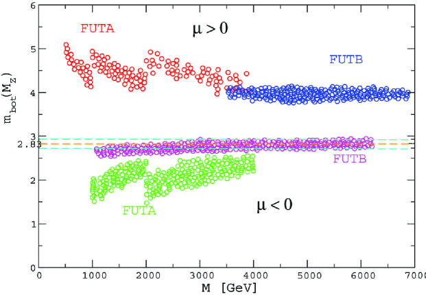
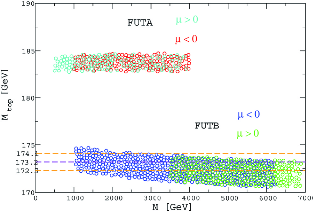
Figure 5.1: The bottom quark mass at the $Z$ boson scale (upper) and top quark pole mass (lower plot) are shown as function of $M$ for both models and both signs of $\mu$.

In Fig. 5.1 we show the FUT A and FUT B predictions for the top pole mass, $M_{\rm top}$, and the running bottom mass at the scale $M_{Z}$, $m_{\rm bot}(M_{Z})$, as a function of the unified gaugino mass $M$, for the two cases $\mu<0$ and $\mu>0$. The running bottom mass is used to avoid the large QCD uncertainties inherent to the pole mass. In the evaluation of the bottom mass $m_{\rm bot}$, we have included the corrections coming from bottom squark-gluino loops and top squark-chargino loops [122]. The prediction is compared to the experimental values [123]

$$m_{b}(M_{Z})=2.83\pm 0.10\,\,\mathrm{GeV}~{}.$$ (5.9)

and

$$m_{t}^{\rm exp}=(173.2\pm 0.9)\,\,\mathrm{GeV}~{}.$$ (5.10)

One can see that the value of $m_{b}$ depends strongly on the sign of $\mu$ due to the above mentioned radiative corrections involving SUSY particles. For both models ${\bf A}$ and ${\bf B}$ the values for $\mu>0$ are above the central experimental value, with $m_{b}(M_{Z})\sim 4.0-5.0$ GeV. For $\mu<0$, on the other hand, model ${\bf B}$ shows overlap with the experimentally measured values, $m_{b}(M_{Z})\sim 2.5-2.8$ GeV. For model ${\bf A}$ we find $m_{b}(M_{Z})\sim 1.5-2.6$ GeV, and there is only a small region of allowed parameter space at large $M$ where we find agreement with the experimental value at the two $\sigma$ level. Therefore, the experimental determination of $m_{b}(M_{Z})$ clearly selects the negative sign of $\mu$.

Now we turn to the top quark mass. The predictions for the top quark mass $M_{t}$ are $\sim 183$ GeV and $\sim 172$ GeV in the models ${\bf A}$ and ${\bf B}$ respectively, as shown in the lower plot of Fig. 5.1. (Here it should be kept in mind that theoretical values for $M_{t}$ may suffer from a correction of $\sim 4\%$ [125, 124, 118]). One can see clearly that model ${\bf B}$ is singled out. In addition the value of $\tan\beta$ is found to be $\tan\beta\sim 54$ and $\sim 48$ for models ${\bf A}$ and ${\bf B}$, respectively. Thus from the comparison of the predictions of the two models with experimental data only FUT B with $\mu<0$ survives.

5.2 Reduction of Couplings in the Minimal Supersymmetric $SU(5)$ GUT

In this section we consider the partial reduction of couplings in the minimal $N=1$ supersymmetric gauge model based on the group SU(5) according to refs [20, 41] The three generations of quarks and leptons are accommodated by three chiral superfields in $\Psi^{I}({\bf 10})$ and $\Phi^{I}(\overline{\bf 5})$, where $I$ runs over the three generations. A $\Sigma({\bf 24})$ is used to break $SU(5)$ down to $SU(3)_{\rm C}\times SU(2)_{\rm L}\times U(1)_{\rm Y}$, and $H({\bf 5})$ and $\overline{H}({\overline{\bf 5}})$ to describe the two Higgs superfields appropriate for electroweak symmetry breaking [126, 127]. Note that the Finite Unified Models discussed in Sect. 5.1 contain four $({\bf 5}+{\bf\bar{5}})$ to describe the Higgs superfields appropriate for electroweak symmetry breaking instead of one set of $({\bf 5}+{\bf\bar{5}})$ used here in the minimal $N=1$ supersymmetric $SU(5)$ version. This minimality makes the present version asymptotically free (negative $\beta_{g}$) instead of finite at one loop, which was the case of the models in Sect. 5.1. The superpotential of the model is [126, 127]

$$\begin{split}W&=\frac{g_{t}}{4}\,\epsilon^{\alpha\beta\gamma\delta\tau}\,\Psi^{(3)}_{\alpha\beta}\Psi^{(3)}_{\gamma\delta}H_{\tau}+\sqrt{2}g_{b}\,\Phi^{(3)\alpha}\Psi^{(3)}_{\alpha\beta}\overline{H}^{\beta}+\frac{g_{\lambda}}{3}\,\Sigma_{\alpha}^{\beta}\Sigma_{\beta}^{\gamma}\Sigma_{\gamma}^{\alpha}+g_{f}\,\overline{H}^{\alpha}\Sigma_{\alpha}^{\beta}H_{\beta}\\ &+\frac{\mu_{\Sigma}}{2}\,\Sigma_{\alpha}^{\gamma}\Sigma_{\gamma}^{\alpha}++\mu_{H}\,\overline{H}^{\alpha}H_{\alpha}~{},\end{split}$$ (5.11)

where $\alpha,\beta,\ldots$ are the $SU(5)$ indices, and we have suppressed the Yukawa couplings of the first two generations. The Lagrangian containing the SSB terms is

$$\begin{split}-{\cal L}_{\rm soft}&=m_{H_{u}}^{2}{\hat{H}}^{*\alpha}{\hat{H}}_{\alpha}+m_{H_{d}}^{2}\hat{\overline{H}}^{*}_{\alpha}\hat{\overline{H}}^{\alpha}+m_{\Sigma}^{2}{\hat{\Sigma}}^{{\dagger}~{}\alpha}_{\beta}{\hat{\Sigma}}_{\alpha}^{\beta}+\sum_{I=1,2,3}\,[\,m_{\Phi^{I}}^{2}{\hat{\Phi}}^{*~{}(I)}_{\alpha}{\hat{\Phi}}^{(I)\alpha}\\ &+\,m_{\Psi^{I}}^{2}{\hat{\Psi}}^{{\dagger}~{}(I)\alpha\beta}{\hat{\Psi}}^{(I)}_{\beta\alpha}\,]+\{\,\frac{1}{2}M\lambda\lambda+B_{H}\hat{\overline{H}}^{\alpha}{\hat{H}}_{\alpha}+B_{\Sigma}{\hat{\Sigma}}^{\alpha}_{\beta}{\hat{\Sigma}}_{\alpha}^{\beta}+h_{f}\,\hat{\overline{H}}^{\alpha}{\hat{\Sigma}}_{\alpha}^{\beta}{\hat{H}}_{\beta}\\ &+\frac{h_{\lambda}}{3}\,{\hat{\Sigma}}_{\alpha}^{\beta}{\hat{\Sigma}}_{\beta}^{\gamma}{\hat{\Sigma}}_{\gamma}^{\alpha}+\frac{h_{t}}{4}\,\epsilon^{\alpha\beta\gamma\delta\tau}\,{\hat{\Psi}}^{(3)}_{\alpha\beta}{\hat{\Psi}}^{(3)}_{\gamma\delta}{\hat{H}}_{\tau}+\sqrt{2}h_{b}\,{\hat{\Phi}}^{(3)\alpha}{\hat{\Psi}^{(3)}}_{\alpha\beta}\hat{\overline{H}}^{\beta}+\mbox{h.c.}\,\}~{},\end{split}$$ (5.12)

where a hat is used to denote the scalar component of each chiral superfield.

The RG functions of this model may be found in refs. [128, 129, 109], and we employ the usual normalization of the RG functions, $d{\rm A}/d\ln\mu~{}=~{}[\beta^{(1)}(A)~{}~{}\mbox{or}~{}~{}\gamma^{(1)}(A)]/16\pi^{2}+\dots$, where $\dots$ are higher orders, and $\mu$ is the renormalization scale:

$$\beta^{(1)}(g) =-3g^{3}~{},~{}\beta^{(1)}(g_{t})=[\,-\frac{96}{5}\,g^{2}+9\,g_{t}^{2}+\frac{24}{5}\,g_{f}^{2}+4\,g_{b}^{2}\,]\,g_{t}~{},$$

$$\beta^{(1)}(g_{b}) =[\,-\frac{84}{5}\,g^{2}+3\,g_{t}^{2}+\frac{24}{5}\,g_{f}^{2}+10\,g_{b}^{2}\,]\,g_{b}~{},$$

$$\beta^{(1)}(g_{\lambda}) =[\,-30\,g^{2}+\frac{63}{5}\,g_{\lambda}^{2}+3\,g_{f}^{2}\,]\,g_{\lambda}~{},$$

$$\beta^{(1)}(g_{f}) =[\,-\frac{98}{5}\,g^{2}+3\,g_{t}^{2}+4\,g_{b}^{2}+\frac{53}{5}\,g_{f}^{2}+\frac{21}{5}\,g_{\lambda}^{2}\,]\,g_{f}~{},~{}\gamma^{(1)}(M)=-6g^{2}\,M~{},$$

$$\gamma^{(1)}(\mu_{\Sigma}) =[\,-20g^{2}+2g_{f}^{2}+\frac{42}{5}g_{\lambda}^{2}\,]\,\mu_{\Sigma}~{},~{}\gamma^{(1)}(\mu_{H})=[\,-\frac{48}{5}g^{2}+\frac{48}{5}g_{f}^{2}+4g_{b}^{2}+3g_{t}^{2}\,]\,\mu_{H}~{},$$

$$\gamma^{(1)}(B_{H}) =[\,-\frac{48}{5}g^{2}+\frac{48}{5}g_{f}^{2}+4g_{b}^{2}+3g_{t}^{2}\,]\,B_{H}$$

$$+[\,\frac{96}{5}g^{2}M+\frac{96}{5}h_{f}g_{f}+8g_{b}h_{b}+6g_{t}h_{t}]\,\mu_{H}~{},$$

$$\gamma^{(1)}(B_{\Sigma}) =[\,-20g^{2}+2g_{f}^{2}+\frac{42}{5}g_{\lambda}^{2}\,]\,B_{\Sigma}+[\,40g^{2}M+4h_{f}g_{f}+\frac{84}{5}g_{\lambda}h_{\lambda}]\,\mu_{\Sigma}~{},$$

$$\gamma^{(1)}(h_{t}) =[\,-\frac{96}{5}\,g^{2}+9\,g_{t}^{2}+\frac{24}{5}\,g_{f}^{2}+4\,g_{b}^{2}\,]\,h_{t}$$

$$+[\,\frac{192}{5}Mg^{2}+18h_{t}g_{t}+8h_{b}g_{b}+\frac{48}{5}h_{f}g_{f}\,]\,g_{t}~{},$$

$$\gamma^{(1)}(h_{b}) =[\,-\frac{84}{5}\,g^{2}+3\,g_{t}^{2}+\frac{24}{5}\,g_{f}^{2}+10\,g_{b}^{2}\,]\,h_{b}$$

$$+[\,\frac{168}{5}Mg^{2}+6h_{t}g_{t}+20h_{b}g_{b}+\frac{48}{5}h_{f}g_{f}\,]\,g_{b}~{}~{},$$

$$\gamma^{(1)}(h_{\lambda}) =[\,-30\,g^{2}+\frac{63}{5}\,g_{\lambda}^{2}+3\,g_{f}^{2}\,]\,h_{\lambda}+[\,60Mg^{2}+\frac{126}{5}h_{\lambda}g_{\lambda}+6h_{f}g_{f}\,]\,g_{\lambda}~{},$$

$$\gamma^{(1)}(h_{f}) =[\,-\frac{98}{5}\,g^{2}+3\,g_{t}^{2}+4\,g_{b}^{2}+\frac{53}{5}\,g_{f}^{2}+\frac{21}{5}\,g_{\lambda}^{2}\,]\,h_{f}$$

$$~{}+[\,\frac{196}{5}Mg^{2}+6h_{t}g_{t}+8h_{b}g_{b}+\frac{42}{5}h_{\lambda}g_{\lambda}+\frac{106}{5}h_{f}g_{f}\,]\,g_{f}~{},$$

$$\gamma^{(1)}(m_{H_{d}}^{2}) =-\frac{96}{5}g^{2}M^{2}+\frac{48}{5}g_{f}^{2}(m_{H_{u}}^{2}+m_{H_{d}}^{2}+m_{\Sigma}^{2})$$

$$+8g_{b}^{2}(m_{H_{d}}^{2}+m_{\Psi^{3}}^{2}+m_{\Phi^{3}}^{2})+\frac{48}{5}h_{f}^{2}+8h_{b}^{2}~{},$$

$$\gamma^{(1)}(m_{H_{u}}^{2}) =-\frac{96}{5}g^{2}M^{2}+\frac{48}{5}g_{f}^{2}(m_{H_{u}}^{2}+m_{H_{d}}^{2}+m_{\Sigma^{3}}^{2})+6g_{t}^{2}(m_{H_{u}}^{2}+2m_{\Psi^{3}}^{2})+\frac{48}{5}h_{f}^{2}+6h_{t}^{2}~{},$$

$$\gamma^{(1)}(m_{\Sigma}^{2}) =-40g^{2}M^{2}+2g_{f}^{2}(m_{H_{u}}^{2}+m_{H_{d}}^{2}+m_{\Sigma}^{2})+\frac{126}{5}g_{\lambda}^{2}m_{\Sigma}^{2}+2h_{f}^{2}+\frac{42}{5}h_{\lambda}^{2}~{},$$

$$\gamma^{(1)}(m_{\Phi^{3}}^{2}) =-\frac{96}{5}g^{2}M^{2}+8g_{b}^{2}(m_{H_{d}}^{2}+m_{\Psi^{3}}^{2}+m_{\Phi^{3}}^{2})+8h_{b}^{2}~{},$$

$$\gamma^{(1)}(m_{\Psi^{3}}^{2}) =-\frac{144}{5}g^{2}M^{2}+6g_{t}^{2}(m_{H_{u}}^{2}+2m_{\Psi^{3}}^{2})+4g_{b}^{2}(m_{H_{d}}^{2}+m_{\Psi^{3}}^{2}+m_{\Phi^{3}}^{2})+6h_{t}^{2}+4h_{b}^{2}~{},$$

$$\gamma^{(1)}(m_{\Phi^{1,2}}^{2}) =-\frac{96}{5}g^{2}M^{2}~{},~{}\gamma^{(1)}(m_{\Psi^{1,2}}^{2})=-\frac{144}{5}g^{2}M^{2}~{},$$ (5.13)

where $g$ stands for the gauge coupling.

The reduction solution is found as follows. We require that the reduced theory should contain the minimal number of the SSB parameters that are consistent with perturbative renormalizability. We will find that the set of the perturbatively unified SSB parameters significantly differ from the so-called universal SSB parameters.

Without loss of generality, one can assume that the gauge coupling $g$ is the primary coupling. Note that the reduction solutions in the dimension-zero sector is independent of the dimensionful sector (under the assumption of a mass independent renormalization scheme). It has been found [128] that there exist two asymptotically free (AF) solutions that make a Gauge-Yukawa Unification possible in the present model:

$$\begin{split}a&:g_{t}=\sqrt{\frac{2533}{2605}}g+{\cal O}(g^{3})~{},~{}g_{b}=\sqrt{\frac{1491}{2605}}g+{\cal O}(g^{3})~{},~{}g_{\lambda}=0~{},~{}g_{f}=\sqrt{\frac{560}{521}}g+{\cal O}(g^{3})~{},\\ b&:g_{t}=\sqrt{\frac{89}{65}}g+{\cal O}(g^{3})~{},~{}g_{b}=\sqrt{\frac{63}{65}}g+{\cal O}(g^{3})~{},~{}g_{\lambda}=0~{},~{}g_{f}=0~{},\end{split}$$ (5.14)

where the higher order terms denote uniquely computable power series in $g$. It has been also found that the two solutions in (5.14) describe the boundaries of an asymptotically free RG-invariant surface in the space of the couplings, on which $g_{\lambda}$ and $g_{f}$ can be different from zero. This observation has enabled us to obtain a partial reduction of couplings for which the $g_{\lambda}$ and $g_{f}$ can be treated as (non-vanishing) independent parameters without loosing AF. Later we have found [130] that the region on the AF surface consistent with the proton decay constraint has to be very close to the solution $a$. Therefore, we assume in the following discussion that we are exactly at the boundary defined by the solution $a$ .

In the dimensionful sector, we seek the reduction of the parameters in the form of Eqs. (2.30). First, one can realize that the supersymmetric mass parameters, $\mu_{\Sigma}$ and $\mu_{H}$, and the gaugino mass parameter $M$ cannot be reduced; that is, there is no solution in the desired form. Therefore, they should be treated as independent parameters. We find the following lowest order reduction solution:

$$B_{H}=\frac{1029}{521}\,\mu_{H}M~{},~{}B_{\Sigma}=-\frac{3100}{521}\,\mu_{\Sigma}M~{},$$ (5.15)

$$\begin{split}h_{t}&=-g_{t}\,M~{},~{}h_{b}=-g_{b}\,M~{},~{}h_{f}=-g_{f}\,M~{},~{}h_{\lambda}=0~{},\\ m_{H_{u}}^{2}&=-\frac{569}{521}M^{2}~{},~{}m_{H_{d}}^{2}=-\frac{460}{521}M^{2}~{},~{}m_{\Sigma}^{2}=\frac{1550}{521}M^{2}~{},\\ m_{\Phi^{3}}^{2}&=\frac{436}{521}M^{2}~{},~{}m_{\Phi^{1,2}}^{2}=\frac{8}{5}M^{2}~{},~{}m_{\Psi^{3}}^{2}=\frac{545}{521}M^{2}~{},~{}m_{\Psi^{1,2}}^{2}=\frac{12}{5}M^{2}~{}.\end{split}$$ (5.16)

So, the gaugino mass parameter $M$ plays a similar role as the gravitino mass $m_{2/3}$ in supergravity coupled GUTs and characterizes the scale of the supersymmetry–breaking.

In addition to the $\mu_{\Sigma}$, $\mu_{H}$ and $M$, it is possible to include also $B_{H}$ and $B_{\Sigma}$ as independent parameters without changing the one-loop reduction solution (5.16).

The prediction of the minimal supersymmetric $SU(5)$ GUT, following the Gauge-Yukawa Unification of the solution a in Eqs (5.14) is:

$$\begin{split}M_{t}&\simeq 1.8\times 10^{2}~{}\mbox{GeV}~{},~{}M_{b}\simeq 5.4~{}\mbox{GeV}~{},~{}\alpha_{3}(M_{Z})\simeq 0.12~{},\\ M_{\rm GUT}&\simeq 1.7\times 10^{16}~{}\mbox{GeV}~{},\alpha_{\rm GUT}\simeq 0.040~{},~{}\tan\beta(M_{\rm SUSY})\simeq 48~{},\end{split}$$

where $M_{t}$ and $M_{b}$ are the physical top and bottom quark masses. These values suffer from corrections coming from different sources such as threshold effects, which are partly taken into account and estimated in Ref. [130]. In Ref. [41], Tab. 1, also the prediction of the specific model for several SSB parameters can be found. Just for completeness we mention that the input parameters for the above prediction were:

$$\alpha_{1}(M_{Z})=0.0169~{},~{}\alpha_{2}(M_{Z})=0.0337~{},~{}\alpha_{\tau}(M_{Z})=8.005\times 10^{-6}~{}$$

while the SUSY scale was fixed at $500$ GeV.

The present model has very good chances to survive the recent experimental constraints. A more detailed examination is in order to determine its viability.

5.3 Gauge-Yukawa Unification in other Supersymmetric GUTs by Reducing the Couplings

5.3.1 Asymptotically Non-Free Pati-Salam Model

In this section a model is discussed, where a partial reduction of couplings is achieved, which however is not based on a single gauge group, but on a product of simple groups. In order for the RGI method for the gauge coupling unification to work, the gauge couplings should have the same asymptotic behavior. Recall that this common behavior is absent in the standard model with three families. A way to achieve a common asymptotic behavior of all the different gauge couplings is to embed $SU(3)_{C}\times SU(2)_{L}\times U(1)_{Y}$ to some non-abelian gauge group, as it was done in the previous sections. However, in this case still a major rôle in the GYU is due to the group theoretical aspects of the covering GUT. Here we would like to examine the power of RGI method by considering theories without covering GUTs. We found [131] that the minimal phenomenologically viable model is based on the gauge group of Pati and Salam [132]– ${\cal G}_{\rm PS}\equiv SU(4)\times SU(2)_{R}\times SU(2)_{L}$. We recall that $N=1$ supersymmetric models based on this gauge group have been studied with renewed interest because they could in principle be derived from superstrings [133, 134].

In our supersymmetric, Gauge-Yukawa unified model based on ${\cal G}_{\rm PS}$ [131], three generations of quarks and leptons are accommodated by six chiral supermultiplets, three in $({\bf 4},{\bf 2},{\bf 1})$ and three $({\bf\overline{4}},{\bf 1},{\bf 2})$, which we denote by $\Psi^{(I)\mu~{}i_{R}}$ and $\overline{\Psi}_{\mu}^{(I)i_{L}}$, ($I$ runs over the three generations, and $\mu,\nu~{}(=1,2,3,4)$ are the $SU(4)$ indices while $i_{R}~{},~{}i_{L}~{}(=1,2)$ stand for the $SU(2)_{L,R}$ indices.) The Higgs supermultiplets in $({\bf 4},{\bf 2},{\bf 1})$, $({\bf\overline{4}},{\bf 2},{\bf 1})$ and $({\bf 15},{\bf 1},{\bf 1})$ are denoted by $H^{\mu~{}i_{R}}~{},~{}\overline{H}_{\mu~{}i_{R}}$ and $\Sigma^{\mu}_{\nu}$, respectively. They are responsible for the spontaneous symmetry breaking (SSB) of $SU(4)\times SU(2)_{R}$ down to $SU(3)_{C}\times U(1)_{Y}$. The SSB of $U(1)_{Y}\times SU(2)_{L}$ is then achieved by the nonzero VEV of $h_{i_{R}i_{L}}$ which is in $({\bf 1},{\bf 2},{\bf 2})$. In addition to these Higgs supermultiplets, we introduce $G^{\mu}_{\nu~{}i_{R}i_{L}}~{}({\bf 15},{\bf 2},{\bf 2})$, $\phi~{}({\bf 1},{\bf 1},{\bf 1})$ and $\Sigma^{{}^{\prime}\mu}_{\nu}~{}({\bf 15},{\bf 1},{\bf 1})$. The $G^{\mu}_{\nu~{}i_{R}i_{L}}$ is introduced to realize the $SU(4)\times SU(2)_{R}\times SU(2)_{L}$ version of the Georgi-Jarlskog type ansatz [135] for the mass matrix of leptons and quarks while $\phi$ is supposed to mix with the right-handed neutrino supermultiplets at a high energy scale. With these things in mind, we write down the superpotential of the model $W$, which is the sum of the following superpotentials:

$$\begin{split}W_{Y}&=\sum_{I,J=1}^{3}g_{IJ}\,\overline{\Psi}^{(I)i_{R}}_{\mu}\,\Psi^{(J)\mu~{}i_{L}}~{}h_{i_{R}i_{L}}~{},~{}\\ W_{GJ}&=g_{GJ}\,\overline{\Psi}^{(2)i_{R}}_{\mu}\,G^{\mu}_{\nu~{}i_{R}j_{L}}\,\Psi^{(2)\nu~{}j_{L}}~{},\\ W_{NM}&=\sum_{I=1,2,3}\,g_{I\phi}~{}\epsilon_{i_{R}j_{R}}\,\overline{\Psi}^{(I)i_{R}}_{\mu}~{}H^{\mu~{}j_{R}}\,\phi~{},\\ W_{SB}&=g_{H}\,\overline{H}_{\mu~{}i_{R}}\,\Sigma^{\mu}_{\nu}\,H^{\nu~{}i_{R}}+\frac{g_{\Sigma}}{3}\,\mbox{Tr}~{}[~{}\Sigma^{3}~{}]+\frac{g_{\Sigma^{\prime}}}{2}\,\mbox{Tr}~{}[~{}(\Sigma^{\prime})^{2}\,\Sigma~{}]~{},\\ W_{TDS}&=\frac{g_{G}}{2}\,\epsilon^{i_{R}j_{R}}\epsilon^{i_{L}j_{L}}\,\mbox{Tr}~{}[~{}G_{i_{R}i_{L}}\,\Sigma\,G_{j_{R}j_{L}}~{}]~{},\\ W_{M}&=m_{h}\,h^{2}+m_{G}\,G^{2}+m_{\phi}\,\phi^{2}+m_{H}\,\overline{H}\,H+m_{\Sigma}\,\Sigma^{2}+m_{\Sigma^{\prime}}\,(\Sigma^{\prime})^{2}~{}.\end{split}$$

Although $W$ has the parity, $\phi\to-\phi$ and $\Sigma^{\prime}\to-\Sigma^{\prime}$, it is not the most general potential, but, as we already mentioned, this is not a problem in N = 1 SUSY theories.

We denote the gauge couplings of $SU(4)\times SU(2)_{R}\times SU(2)_{L}$ by $\alpha_{4}~{},~{}\alpha_{2R}$ and $\alpha_{2L}$, respectively. The gauge coupling for $U(1)_{Y}$, $\alpha_{1}$, normalized in the usual GUT inspired manner, is given by $1/\alpha_{1}~{}=~{}2/5\alpha_{4}+3/5\alpha_{2R}~{}$. In principle, the primary coupling can be any one of the couplings. But it is more convenient to choose a gauge coupling as the primary one because the one-loop $\beta$ functions for a gauge coupling depends only on its own gauge coupling. For the present model, we use $\alpha_{2L}$ as the primary one. Since the gauge sector for the one-loop $\beta$ functions is closed, the solutions of the fixed point equations (2.22) are independent on the Yukawa and Higgs couplings. One easily obtains $\rho_{4}^{(1)}=8/9~{},~{}\rho_{2R}^{(1)}~{}=~{}4/5$, so that the RGI relations (2.26) at the one-loop level become

$$\tilde{\alpha}_{4} = \frac{\alpha_{4}}{\alpha_{2L}}~{}=~{}\frac{8}{9}~{},~{}\tilde{\alpha}_{1}~{}=~{}\frac{\alpha_{1}}{\alpha_{2L}}~{}=~{}\frac{5}{6}~{}.$$ (5.17)

The solutions in the Yukawa-Higgs sector strongly depend on the result of the gauge sector. After slightly involved algebraic computations, one finds that most predictive solutions contain at least three vanishing $\rho_{i}^{(1)}$’s. Out of these solutions, there are two that exhibit the most predictive power and moreover they satisfy the neutrino mass relation $m_{\nu_{\tau}}>m_{\nu_{\mu}}~{},~{}m_{\nu_{e}}$. For the first solution we have $\rho_{1\phi}^{(1)}=\rho_{2\phi}^{(1)}=\rho_{\Sigma}^{(1)}=0$, while for the second solution, $\rho_{1\phi}^{(1)}=\rho_{2\phi}^{(1)}=\rho_{G}^{(1)}=0$, and one finds that for the cases above the power series solutions (2.26) take the form

$$\begin{split}\tilde{\alpha}_{GJ}&\simeq\left\{\begin{array}[]{l}1.67-0.05\tilde{\alpha}_{1\phi}+0.004\tilde{\alpha}_{2\phi}-0.90\tilde{\alpha}_{\Sigma}+\cdots\\ 2.20-0.08\tilde{\alpha}_{2\phi}-0.05\tilde{\alpha}_{G}+\cdots\end{array}\right.~{}~{},\\ \tilde{\alpha}_{33}&\simeq\left\{\begin{array}[]{l}3.33+0.05\tilde{\alpha}_{1\phi}+0.21\tilde{\alpha}_{2\phi}-0.02\tilde{\alpha}_{\Sigma}+\cdots\\ 3.40+0.05\tilde{\alpha}_{1\phi}-1.63\tilde{\alpha}_{2\phi}-0.001\tilde{\alpha}_{G}+\cdots\end{array}\right.~{}~{},\\ \tilde{\alpha}_{3\phi}&\simeq\left\{\begin{array}[]{l}1.43-0.58\tilde{\alpha}_{1\phi}-1.43\tilde{\alpha}_{2\phi}-0.03\tilde{\alpha}_{\Sigma}+\cdots\\ 0.88-0.48\tilde{\alpha}_{1\phi}+8.83\tilde{\alpha}_{2\phi}+0.01\tilde{\alpha}_{G}+\cdots\end{array}\right.~{}~{},\\ \tilde{\alpha}_{H}&\simeq\left\{\begin{array}[]{l}1.08-0.03\tilde{\alpha}_{1\phi}+0.10\tilde{\alpha}_{2\phi}-0.07\tilde{\alpha}_{\Sigma}+\cdots\\ 2.51-0.04\tilde{\alpha}_{1\phi}-1.68\tilde{\alpha}_{2\phi}-0.12\tilde{\alpha}_{G}+\cdots\end{array}\right.~{}~{},~{}~{}\\ \tilde{\alpha}_{\Sigma}&\simeq\left\{\begin{array}[]{l}---\\ 0.40+0.01\tilde{\alpha}_{1\phi}-0.45\tilde{\alpha}_{2\phi}-0.10\tilde{\alpha}_{G}+\cdots\end{array}\right.~{},\\ \tilde{\alpha}_{\Sigma^{\prime}}&\simeq\left\{\begin{array}[]{ll}4.91-0.001\tilde{\alpha}_{1\phi}-0.03\tilde{\alpha}_{2\phi}-0.46\tilde{\alpha}_{\Sigma}+\cdots\\ 8.30+0.01\tilde{\alpha}_{1\phi}+1.72\tilde{\alpha}_{2\phi}-0.36\tilde{\alpha}_{G}+\cdots\end{array}\right.~{}~{},\\ \tilde{\alpha}_{G}&\simeq\left\{\begin{array}[]{ll}5.59+0.02\tilde{\alpha}_{1\phi}-0.04\tilde{\alpha}_{2\phi}-1.33\tilde{\alpha}_{\Sigma}+\cdots\\ ---\end{array}\right.~{}~{}.\end{split}$$ (5.18)

We have assumed that the Yukawa couplings $g_{IJ}$ except for $g_{33}$ vanish. They can be included into RGI relations as small perturbations, but their numerical effects will be rather small.

The number $N_{H}$ of the Higgses lighter than $M_{\rm SUSY}$ could vary from one to four while the number of those to be taken into account above $M_{\rm SUSY}$ is fixed at four. We have assumed here that $N_{H}=1$. The dependence of the top mass on $M_{\rm SUSY}$ in this model is shown in Fig. 5.2. One can see that for any reasonable supersymmetry breaking scale in the TeV region the experimentally found top quark mass cannot be reproduced within this model.

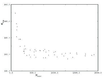
Figure 5.2: The values for $M_{t}$ predicted by the Pati-Salam model for different $M_{\rm SUSY}$ scales.

5.3.2 Asymptotically Non-Free $SO(10)$ Model

In this section a model based on SO(10) is discussed, which also admits a partial reduction of couplings [136]. We denote the hermitean $SO(10)$-gamma matrices by $\Gamma_{\alpha}~{},~{}\alpha=1,\cdots,10$. The charge conjugation matrix $C$ satisfies $C=C^{-1}~{},~{}C^{-1}\,\Gamma_{\alpha}^{T}\,C~{}=~{}-\Gamma_{\alpha}$, and the $\Gamma_{11}$ is defined as $\Gamma_{11}\equiv(-i)^{5}\,\Pi_{\alpha=1}^{10}\Gamma_{\alpha}~{}~{}\mbox{with}~{}~{}(\Gamma_{11})^{2}~{}=~{}1$. The chiral projection operators are given by ${\cal P}_{\pm}=\frac{1}{2}(\,1\pm\Gamma_{11})$.

In $SO(10)$ GUTs [137, 138, 139], three generations of quarks and leptons are accommodated by three chiral supermultiplets in ${\bf 16}$ which we denote by

$$\Psi^{I}({\bf 16})~{}~{}\mbox{with}~{}~{}{\cal P}_{+}\,\Psi^{I}~{}=~{}\Psi^{I}~{},$$ (5.19)

where $I$ runs over the three generations and the spinor index is suppressed. To break $SO(10)$ down to $SU(3)_{\rm C}\times SU(2)_{\rm L}\times U(1)_{\rm Y}$, we use the following set of chiral superfields:

$$S_{\{\alpha\beta\}}({\bf 54})~{},~{}A_{[\alpha\beta]}({\bf 45})~{},~{}\phi({\bf 16})~{},~{}\overline{\phi}({\overline{\bf 16}})~{}.$$ (5.20)

The two $SU(2)_{\rm L}$ doublets which are responsible for the spontaneous symmetry breaking (SSB) of $SU(2)_{\rm L}\times U(1)_{\rm Y}$ down to $U(1)_{\rm EM}$ are contained in $H_{\alpha}({\bf 10})$. We further introduce a singlet $\varphi$ which after the SSB of $SO(10)$ will mix with the right-handed neutrinos so that they will become superheavy.

The superpotential of the model is given by

$$W = W_{Y}+W_{SB}+W_{HS}+W_{NM}+W_{M}~{},$$ (5.21)

where

$$W_{Y} =\frac{1}{2}\sum_{I,J=1}^{3}g_{IJ}\,\Psi^{I}\,C\Gamma_{\alpha}\,\Psi^{J}~{}H_{\alpha}~{},$$

$$W_{SB} =\frac{g_{\phi}}{2}\,\overline{\phi}\,\Gamma_{[\alpha\beta]}\,\phi~{}A_{[\alpha\beta]}+\frac{g_{S}}{3!}\,\mbox{Tr}~{}S^{3}+\frac{g_{A}}{2}\,\mbox{Tr}~{}A^{2}\,S~{},$$

$$W_{HS} =\frac{g_{HS}}{2}\,\ H_{\alpha}\,S_{\{\alpha\beta\}}\,H_{\beta}~{},~{}W_{NM}^{I}~{}=~{}\sum_{I=1}^{3}\,g_{INM}\,\Psi^{I}\,\overline{\phi}\,\varphi~{},$$

$$W_{M} =\frac{m_{H}}{2}\,H^{2}+m_{\varphi}\,\varphi^{2}+m_{\phi}\,\overline{\phi}\phi+\frac{m_{S}}{2}\,S^{2}+\frac{m_{A}}{2}\,A^{2}~{},$$ (5.22)

and $\Gamma_{[\alpha\beta]}=i(\Gamma_{\alpha}\Gamma_{\beta}-\Gamma_{\beta}\Gamma_{\alpha})/2$. As in the case of the $SU(5)$ minimal model, the superpotential is not the most general one, but this does not contradict the philosophy of the coupling unification by the reduction method. $W_{SB}$ is responsible for the SSB of $SO(10)$ down to $SU(3)_{C}\times SU(2)_{W}\times U(1)_{Y}$, and this can be achieved without breaking supersymmetry, while $W_{HS}$ is responsible for the triplet-doublet splitting of $H$. The right-handed neutrinos obtain a superheavy mass through $W_{NM}$ after the SSB, and the Yukawa couplings for the leptons and quarks are contained in $W_{Y}$. We assume that there exists a choice of soft supersymmetry breaking terms so that all the vacuum expectation values necessary for the desired SSB corresponds to the minimum of the potential.

Given the supermultiplet content and the superpotential $W$, we can compute the $\beta$ functions of the model. The gauge coupling of $SO(10)$ is denoted by $g$, and our normalization of the $\beta$ functions is as usual, i.e., $dg_{i}/d\ln\mu~{}=~{}\beta^{(1)}_{i}/16\pi^{2}+O(g^{5})$, where $\mu$ is the renormalization scale. We find:

$$\begin{split}\beta^{(1)}_{g}&=7\,g^{3}~{},\\ \beta^{\left(1\right)}_{g_{T}}&=g_{T}\,\left(\,14g_{T}^{2}+\frac{27}{5}g_{HS}^{2}+g_{3NM}^{2}-\frac{63}{2}g^{2}\,\right)~{},\\ \beta^{\left(1\right)}_{g_{\phi}}&=g_{\phi}\left(\,53g_{\phi^{2}}+\frac{48}{5}g_{A}^{2}+\frac{1}{2}g_{1NM}^{2}+\frac{1}{2}g_{2NM}^{2}+\frac{1}{2}g_{3NM}^{2}-\frac{77}{2}g^{2}\,\right),\\ \beta^{\left(1\right)}_{S}&=g_{S}\left(\,\frac{84}{5}g_{S}^{2}+12g_{A}^{2}+\frac{3}{2}g_{HS}^{2}-60g^{2}\,\right)~{},\\ \beta^{\left(1\right)}_{A}&=g_{A}\left(\,16g_{\phi}^{2}+\frac{28}{5}g_{S}^{2}+\frac{116}{5}g_{A}^{2}+\frac{1}{2}g_{HS}^{2}-52g^{2}\,\right)~{},\\ \beta^{\left(1\right)}_{HS}&=g_{HS}\left(\,8g_{T}^{2}+\frac{28}{5}g_{S}^{2}+4g_{A}^{2}+\frac{113}{10}g_{HS}^{2}-38g^{2}\,\right)~{},\\ \beta^{\left(1\right)}_{1NM}&=g_{1NM}\left(\,\frac{45}{2}g_{\phi}^{2}+9g_{1NM}^{2}+\frac{17}{2}g_{2NM}^{2}+\frac{17}{2}g_{3NM}^{2}-\frac{45}{2}g^{2}\,\right)~{},\\ \beta^{\left(1\right)}_{2NM}&=g_{2NM}\left(\,\frac{45}{2}g_{\phi}^{2}+\frac{17}{2}g_{1NM}^{2}+9g_{2NM}^{2}+\frac{17}{2}g_{3NM}^{2}-\frac{45}{2}g^{2}\,\right)~{},\\ \beta^{\left(1\right)}_{3NM}&=g_{3NM}\left(\,5g_{T}^{2}+\frac{45}{2}g_{\phi}^{2}+\frac{17}{2}g_{1NM}^{2}+\frac{17}{2}g_{2NM}^{2}+9g_{3NM}^{2}-\frac{45}{2}g^{2}\,\right)~{}.\end{split}$$ (5.23)

We have assumed that the Yukawa couplings $g_{IJ}$ except for $g_{T}\equiv g_{33}$ vanish. They can be included as small perturbations. Needless to say that the soft susy breaking terms do not alter the $\beta$ functions above.

We find that there exist two independent solutions, $A$ and $B$, that have the most predictive power, where we have chosen the $SO(10)$ gauge coupling as the primary coupling:

$$\rho_{T} =\left\{\begin{array}[]{ll}163/60&\simeq 2.717\\ 0&\end{array}\right.~{}~{},~{}~{}\rho_{\phi}~{}=~{}\left\{\begin{array}[]{ll}5351/9180&\simeq 0.583\\ 1589/2727&\simeq 0.583\end{array}\right.~{},$$ (5.28)

$$\rho_{S} =\left\{\begin{array}[]{ll}152335/51408&\simeq 2.963\\ 850135/305424&\simeq 2.783\end{array}\right.,\rho_{A}=\left\{\begin{array}[]{ll}31373/22032&\simeq 1.424\\ 186415/130896&\simeq 1.424\end{array}\right.,$$ (5.33)

$$\rho_{HS} =\left\{\begin{array}[]{ll}7/81&\simeq 0.086\\ 170/81&\simeq 2.099\end{array}\right.~{},~{}\rho_{1NM}=\rho_{2NM}=\left\{\begin{array}[]{ll}191/204&\simeq 0.936\\ 191/303&\simeq 0.630\end{array}\right.~{}~{},$$ (5.38)

$$\rho_{3NM} =\left\{\begin{array}[]{ll}0&\\ 191/303&\simeq 0.630\end{array}\right.~{}~{}~{}\mbox{for}~{}~{}\left\{\begin{array}[]{l}A\\ B\end{array}\right.~{}.$$ (5.43)

Clearly, the solution B has less predictive power because $\rho_{T}=0$. So, we consider below only the solution A, in which the coupling $\alpha_{3NM}$ should be regarded as a small perturbation because $\rho_{3NM}=0$.

Given this solution it is possible to show, as in the case of $SU(5)$, that the $\rho$’s can be uniquely computed in any finite order in perturbation theory.

The corrections to the reduced couplings coming from the small perturbations up to and including terms of $O(\tilde{\alpha}_{3NM}^{2}$) are:

$$\begin{split}\tilde{\alpha}_{T}&=(\,163/60-0.108\cdots\tilde{\alpha}_{3NM}+0.482\cdots\tilde{\alpha}_{3NM}^{2}+\cdots\,)+\cdots~{},\\ \tilde{\alpha}_{\phi}&=(\,5351/9180+0.316\cdots\tilde{\alpha}_{3NM}+0.857\cdots\tilde{\alpha}_{3NM}^{2}+\cdots\,)+\cdots~{},\\ \tilde{\alpha}_{S}&=(\,152335/51408+0.573\cdots\tilde{\alpha}_{3NM}+5.7504\cdots\tilde{\alpha}_{3NM}^{2}+\cdots\,)+\cdots~{},\\ \tilde{\alpha}_{A}&=(\,31373/22032-0.591\cdots\tilde{\alpha}_{3NM}-4.832\cdots\tilde{\alpha}_{3NM}^{2}+\cdots\,)+\cdots~{},\\ \tilde{\alpha}_{HS}&=(7/81-0.00017\cdots\tilde{\alpha}_{3NM}+0.056\cdots\tilde{\alpha}_{3NM}^{2}+\cdots\,)+\cdots~{},\\ \tilde{\alpha}_{1NM}&=\tilde{\alpha}_{2NM}=(\,191/204-4.473\cdots\tilde{\alpha}_{3NM}+2.831\cdots\tilde{\alpha}_{3NM}^{2}+\cdots\,)+\cdots,\end{split}$$ (5.44)

where $\cdots$ indicates higher order terms which can be uniquely computed. In the partially reduced theory defined above, we have two independent couplings, $\alpha$ and $\alpha_{3NM}$ (along with the Yukawa couplings $\alpha_{IJ}~{},~{}I,J\neq T$).

At the one-loop level, Eq. (5.44) defines a line parametrized by $\tilde{\alpha}_{3NM}$ in the $7$ dimensional space of couplings. A numerical analysis shows that this line blows up in the direction of $\tilde{\alpha}_{S}$ at a finite value of $\tilde{\alpha}_{3NM}$ [136]. So if we require $\tilde{\alpha}_{S}$ to remain within the perturbative regime (i.e., $g_{S}\leq 2$, which means $\tilde{\alpha}_{S}\leq 8$ because $\alpha_{\rm GUT}\sim 0.04$), the $\tilde{\alpha}_{3NM}$ should be restricted to be below $\sim 0.067$. As a consequence, the value of $\tilde{\alpha}_{T}$ is also bounded

$$2.714\leq\tilde{\alpha}_{T}\leq 2.736~{}.$$ (5.45)

This defines GYU boundary conditions holding at the unification scale $M_{\rm GUT}$ in addition to the group theoretical one, $\alpha_{T}=\alpha_{t}~{}=~{}\alpha_{b}~{}=~{}\alpha_{\tau}$. The value of $\tilde{\alpha}_{T}$ is practically fixed so that we may assume that $\tilde{\alpha}_{T}=163/60\simeq 2.72$, which is the unperturbed value.

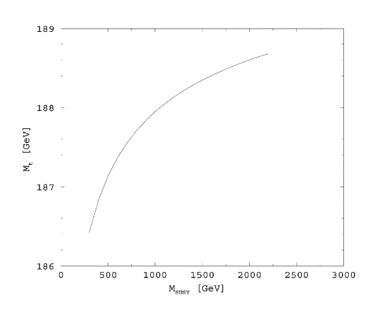
Figure 5.3: Top quark mass prediction versus $M_{\rm SUSY}$ for $\tilde{\alpha}_{T}=2.717$.

Fig. 5.3 shows the prediction for the top quark mass in this model for different values of the supersymmetry breaking scale $M_{\rm SUSY}$. While the value for the top quark mass predicted is below its infrared value ($\sim 189\,\,\mathrm{GeV}$) [136], it is above the experimental value [140]. Consequently, also this particular model has difficulties to meet the experimental data on the top quark mass, despite the theoretical uncertainties involved.

5.4 Finite $SU(N)^{3}$ Unification

We continue examining the possibility of constructing realistic FUTs based on product gauge groups. Consider an $N=1$ supersymmetric theory, with gauge group $SU(N)_{1}\times SU(N)_{2}\times\cdots\times SU(N)_{k}$, with $n_{f}$ copies (number of families) of the supersymmetric multiplets $(N,N^{*},1,\dots,1)+(1,N,N^{*},\dots,1)+\cdots+(N^{*},1,1,\dots,N)$. The one-loop $\beta$-function coefficient in the renormalization-group equation of each $SU(N)$ gauge coupling is simply given by

$$b=\left(-\frac{11}{3}+\frac{2}{3}\right)N+n_{f}\left(\frac{2}{3}+\frac{1}{3}\right)\left(\frac{1}{2}\right)2N=-3N+n_{f}N\,.$$ (5.46)

This means that $n_{f}=3$ is the only solution of Eq.(5.46) that yields $b=0$. Since $b=0$ is a necessary condition for a finite field theory, the existence of three families of quarks and leptons is natural in such models, provided the matter content is exactly as given above.

The model of this type with best phenomenology is the $SU(3)^{3}$ model discussed in Ref. [141], where the details of the model are given. It corresponds to the well-known example of $SU(3)_{C}\times SU(3)_{L}\times SU(3)_{R}$ [142, 143, 144, 145], with quarks transforming as

$$q=\begin{pmatrix}d&u&h\\ d&u&h\\ d&u&h\end{pmatrix}\sim(3,3^{*},1),~{}~{}~{}q^{c}=\begin{pmatrix}d^{c}&d^{c}&d^{c}\\ u^{c}&u^{c}&u^{c}\\ h^{c}&h^{c}&h^{c}\end{pmatrix}\sim(3^{*},1,3),$$ (5.47)

and leptons transforming as

$$\lambda=\begin{pmatrix}N&E^{c}&\nu\\ E&N^{c}&e\\ \nu^{c}&e^{c}&S\end{pmatrix}\sim(1,3,3^{*}).$$ (5.48)

Switching the first and third rows of $q^{c}$ together with the first and third columns of $\lambda$, we obtain the alternative left-right model first proposed in Ref. [145] in the context of superstring-inspired $E_{6}$.

In order for all the gauge couplings to be equal at an energy scale, $M_{\rm GUT}$, the cyclic symmetry $Z_{3}$ must be imposed, i.e.

$$q\to\lambda\to q^{c}\to q,$$ (5.49)

where $q$ and $q^{c}$ are given in eq. (5.47) and $\lambda$ in eq. (5.48). Then, the first of the finiteness conditions (4.5) for one-loop finiteness, namely the vanishing of the gauge $\beta$-function is satisfied.

Next let us consider the second condition, i.e. the vanishing of the anomalous dimensions of all superfields, eq. (4.6). To do that first we have to write down the superpotential. If there is just one family, then there are only two trilinear invariants, which can be constructed respecting the symmetries of the theory, and therefore can be used in the superpotential as follows

$$f~{}Tr(\lambda q^{c}q)+\frac{1}{6}f^{\prime}~{}\epsilon_{ijk}\epsilon_{abc}(\lambda_{ia}\lambda_{jb}\lambda_{kc}+q^{c}_{ia}q^{c}_{jb}q^{c}_{kc}+q_{ia}q_{jb}q_{kc}),$$ (5.50)

where $f$ and $f^{\prime}$ are the Yukawa couplings associated to each invariant. Quark and leptons obtain masses when the scalar parts of the superfields $(\tilde{N},\tilde{N}^{c})$ obtain vacuum expectation values (vevs),

$$m_{d}=f\langle\tilde{N}\rangle,~{}~{}m_{u}=f\langle\tilde{N}^{c}\rangle,~{}~{}m_{e}=f^{\prime}\langle\tilde{N}\rangle,~{}~{}m_{\nu}=f^{\prime}\langle\tilde{N}^{c}\rangle.$$ (5.51)

With three families, the most general superpotential contains 11 $f$ couplings, and 10 $f^{\prime}$ couplings, subject to 9 conditions, due to the vanishing of the anomalous dimensions of each superfield. The conditions are the following

$$\sum_{j,k}f_{ijk}(f_{ljk})^{*}+\frac{2}{3}\sum_{j,k}f^{\prime}_{ijk}(f^{\prime}_{ljk})^{*}=\frac{16}{9}g^{2}\delta_{il}\,,$$ (5.52)

where

$$f_{ijk}=f_{jki}=f_{kij},$$ (5.53)

$$f^{\prime}_{ijk}=f^{\prime}_{jki}=f^{\prime}_{kij}=f^{\prime}_{ikj}=f^{\prime}_{kji}=f^{\prime}_{jik}.$$ (5.54)

Quarks and leptons receive masses when the scalar part of the superfields $\tilde{N}_{1,2,3}$ and $\tilde{N}^{c}_{1,2,3}$ obtain vevs as follows

$$({\cal M}_{d})_{ij}=\sum_{k}f_{kij}\langle\tilde{N}_{k}\rangle,~{}~{}~{}({\cal M}_{u})_{ij}=\sum_{k}f_{kij}\langle\tilde{N}^{c}_{k}\rangle,$$ (5.55)

$$({\cal M}_{e})_{ij}=\sum_{k}f^{\prime}_{kij}\langle\tilde{N}_{k}\rangle,~{}~{}~{}({\cal M}_{\nu})_{ij}=\sum_{k}f^{\prime}_{kij}\langle\tilde{N}^{c}_{k}\rangle.$$ (5.56)

We will assume that the below $M_{\rm GUT}$ we have the usual MSSM , with the two Higgs doublets coupled maximally to the third generation. Therefore we have to choose the linear combinations $\tilde{N}^{c}=\sum_{i}a_{i}\tilde{N}^{c}_{i}$ and $\tilde{N}=\sum_{i}b_{i}\tilde{N}_{i}$ to play the role of the two Higgs doublets, which will be responsible for the electroweak symmetry breaking. This can be done by choosing appropriately the masses in the superpotential [114], since they are not constrained by the finiteness conditions. We choose that the two Higgs doublets are predominately coupled to the third generation. Then these two Higgs doublets couple to the three families differently, thus providing the freedom to understand their different masses and mixings. The remnants of the $SU(3)^{3}$ FUT are the boundary conditions on the gauge and Yukawa couplings, i.e. Eq.(5.52), the $h=-MC$ relation, and the soft scalar-mass sum rule eq. (5.8) at $M_{\rm GUT}$, which, when applied to the present model, takes the form

$$m^{2}_{H_{u}}+m^{2}_{\tilde{t}^{c}}+m^{2}_{\tilde{q}}=M^{2}=m^{2}_{H_{d}}+m^{2}_{\tilde{b}^{c}}+m^{2}_{\tilde{q}}~{},$$ (5.57)

where ${\tilde{t}^{c}},~{}{\tilde{b}^{c}}$, and ${\tilde{q}}$ are the scalar parts of the corresponding superfields.

Concerning the solution to Eq.(5.52) we consider two versions of the model:
I) An all-loop finite model with a unique and isolated solution, in which $f^{\prime}$ vanishes, which leads to the following relations

$$f^{2}=f^{2}_{111}=f^{2}_{222}=f^{2}_{333}=\frac{16}{9}g^{2}\,.$$ (5.58)

As for the lepton masses, since all $f^{\prime}$ couplings have been fixed to be zero at this order, in principle they would be expected to appear radiatively induced by the scalar lepton masses appearing in the SSB sector of the theory. However, due to the finiteness conditions they cannot appear radiatively and remain as a problem for further study.
II) A two-loop finite solution, in which we keep $f^{\prime}$ non-vanishing and we use it to introduce the lepton masses. The model in turn becomes finite only up to two-loops since the corresponding solution of Eq.(5.52) is not an isolated one any more, i.e. it is a parametric one. In this case we have the following boundary conditions for the Yukawa couplings

$$f^{2}=r\left(\frac{16}{9}\right)g^{2}\,,\quad f^{\prime 2}=(1-r)\left(\frac{8}{3}\right)g^{2}\,,$$ (5.59)

where $r$ is a free parameter which parametrizes the different solutions to the finiteness conditions. As for the boundary conditions of the soft scalars, we have the universal case.

Below $M_{\rm GUT}$ all couplings and masses of the theory run according to the RGEs of the MSSM. Thus we examine the evolution of these parameters according to their RGEs up to two-loops for dimensionless parameters and at one-loop for dimensionful ones imposing the corresponding boundary conditions. We further assume a unique SUSY breaking scale $M_{\rm SUSY}$ and below that scale the effective theory is just the SM.

We compare our predictions with the experimental value of $m_{t}^{\rm exp}$ and recall that the theoretical values for $m_{t}$ suffer from a correction of $\sim 4\%$ [125, 124, 118]. In the case of the bottom quark, we take again the value evaluated at $M_{Z}$, see Eq. (5.9). In the case of model I, the predictions for the top quark mass (in this case $m_{b}$ is an input) $m_{t}$ are $\sim 183\,{\rm~{}GeV}$ for $\mu<0$, which is above the experimental value, and there are no solutions for $\mu>0$.

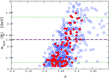
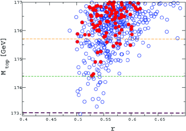
Figure 5.4: The figures show the values for the top and bottom quark masses for the FUT model $SU(3)^{3}$, with $\mu<0$, vs the parameter $r$. The thicker horizontal line is the experimental central value, and the lighter green and orange ones are the one and two sigma limits respectively. The red points are the ones that satisfy the $B$-physics constraints, as discussed in Chapter 6.

For the two-loop model II, we look for the values of the parameter $r$ which comply with the experimental limits given above for top and bottom quarks masses. In the case of $\mu>0$, for the bottom quark, the values of $r$ lie in the range $0.15\lesssim r\lesssim 0.32$. For the top mass, the range of values for r is $0.35\lesssim r\lesssim 0.6$. From these values we can see that there is a very small region where both top and bottom quark masses are in the experimental range for the same value of $r$. In the case of $\mu<0$ the situation is similar, although slightly better, with the range of values $0.62\lesssim r\lesssim 0.77$ for the bottom mass, and $0.4\lesssim r\lesssim 0.62$ for the top quark mass. In the above mentioned analysis, the masses of the new particles $h$’s and $E$’s of all families were taken to be at the $M_{\rm GUT}$ scale.

Taking into account new thresholds for these exotic particles below $M_{\rm GUT}$ we find a wider phenomenologically viable parameter space [148]. This can be seen in Fig. 5.4, where we took only one down-like exotic particle decoupling at $10^{14}$ GeV, below than the usual MSSM.

In this case, for $r\sim 0.5\sim 0.62$ we have reasonable agreement with experimental data for both top and bottom quark masses, where the red points in the figure are the ones that satisfy the $B$-physics constraints (at the time of the analysis) [149]. The above analysis shows that it is worth returning with a fresh examination of this model taking into account all new experimental constraints.

5.5 Reduction of Couplings in the MSSM

In this section we are working in the framework of MSSM, assuming though the existence of a covering GUT.

The analysis of the partial reduction of couplings in this framework was first done in refs [150, 151].

The superpotential of the MSSM (where again we restrict ourselves to the third generation of fermions) is defined by

$$W=Y_{t}H_{2}Qt^{c}+Y_{b}H_{1}Qb^{c}+Y_{\tau}H_{1}L\tau^{c}+\mu H_{1}H_{2}\,,$$ (5.60)

where $Q,L,t,b,\tau,H_{1},H_{2}$ are the usual superfields of MSSM, while the SSB Lagrangian is given by

$$\begin{split}-\mathcal{L}_{\rm SSB}&=\sum_{\phi}m^{2}_{\phi}\hat{\phi^{*}}\hat{\phi}+\left[m^{2}_{3}\hat{H_{1}}\hat{H_{2}}+\sum_{i=1}^{3}\frac{1}{2}M_{i}\lambda_{i}\lambda_{i}+\textrm{h.c}\right]\\ &+\left[h_{t}\hat{H_{2}}\hat{Q}\hat{t^{c}}+h_{b}\hat{H_{1}}\hat{Q}\hat{b^{c}}+h_{\tau}\hat{H_{1}}\hat{L}\hat{\tau^{c}}+\textrm{h.c.}\right],\end{split}$$ (5.61)

where $\hat{\phi}$ represents the scalar component of all superfields, $\lambda$ refers to the gaugino fields while all hatted fields refer to the scalar components of the corresponding superfield. The Yukawa $Y_{t,b,\tau}$ and the trilinear $h_{t,b,\tau}$ couplings refer to the third generator only, neglecting the first two generations.

Let us start with the dimensionless couplings, i.e. gauge and Yukawa. As a first step we consider only the strong coupling and the top and bottom Yukawa couplings, while the other two gauge couplings and the tau Yukawa will be treated as corrections. Following the above line, we reduce the Yukawa couplings in favour of the strong coupling $\alpha_{3}$

$$\frac{Y^{2}_{i}}{4\pi}\equiv\alpha_{i}=G_{i}^{2}\alpha_{3},\qquad i=t,b,$$

and using the RGE for the Yukawa, we get

$$G_{i}^{2}=\frac{1}{3},\qquad i=t,b.$$

This system of the top and bottom Yukawa couplings reduced with the strong one is dictated by (i) the different running behaviour of the $SU(2)$ and $U(1)$ coupling compared to the strong one [26] and (ii) the incompatibility of applying the above reduction for the tau Yukawa since the corresponding $G^{2}$ turns negative [152]. Adding now the two other gauge couplings and the tau Yukawa in the RGE as corrections, we obtain

$$G_{t}^{2}=\frac{1}{3}+\frac{71}{525}\rho_{1}+\frac{3}{7}\rho_{2}+\frac{1}{35}\rho_{\tau},\qquad G_{b}^{2}=\frac{1}{3}+\frac{29}{525}\rho_{1}+\frac{3}{7}\rho_{2}-\frac{6}{35}\rho_{\tau}$$ (5.62)

where

$$\rho_{1,2}=\frac{g_{1,2}^{2}}{g_{3}^{2}}=\frac{\alpha_{1,2}}{\alpha_{3}},\qquad\rho_{\tau}=\frac{g_{\tau}^{2}}{g_{3}^{2}}=\frac{\displaystyle{\frac{Y^{2}_{\tau}}{4\pi}}}{\alpha_{3}}$$ (5.63)

Note that the corrections in Eq.(5.62) are taken at the GUT scale and under the assumption that

$$\frac{d}{dg_{3}}\left(\frac{Y_{t,b}^{2}}{g_{3}^{2}}\right)=0.$$

Let us comment on our assumption above, which led to the Eq.(5.62). In practice we assume that even including the corrections from the rest of the gauge as well as the tau Yukawa couplings, at the GUT scale the ratio of the top and bottom couplings $\alpha_{t,b}$ over the strong coupling are still constant, i.e. their scale dependence is negligible. Or, rephrasing it, our assumption can be understood as a requirement that in the ultraviolet (close to the GUT scale) the ratios of the top and bottom Yukawa couplings over the strong coupling become least sensitive against the change of the renormalization scale. This requirement sets the boundary condition at the GUT scale, given in Eq.(5.62). Alternatively one could follow the systematic method to include the corrections to a non-trivially reduced system developed in ref. [27], but considering two reduced systems: the first one consisting of the “top, bottom” couplings and the second of the “strong, bottom” ones.

In the next order the corrections are assumed to be in the form

$$\alpha_{i}=G_{i}^{2}\alpha_{3}+J_{i}^{2}\alpha_{3}^{2},\qquad i=t,b.$$

Then, the coefficients $J_{i}$ are given by

$$J_{i}^{2}=\frac{1}{4\pi}\,\frac{17}{24},\qquad i=t,b$$

for the case where only the strong gauge and the top and bottom Yukawa couplings are active, while for the case where the other two gauge and the tau Yukawa couplings are added as corrections we obtain

$$J_{t}^{2}=\frac{1}{4\pi}\frac{N_{t}}{D},\quad J_{b}^{2}=\frac{1}{4\pi}\frac{N_{b}}{5D},$$

where

$$\begin{split}D=&257250(196000+44500\rho_{1}+2059\rho_{1}^{2}+200250\rho_{2}+22500\rho_{1}\rho_{2}+50625\rho_{2}^{2}-\\ &33375\rho_{\tau}-5955\rho_{1}\rho_{\tau}-16875\rho_{2}\rho_{\tau}-1350\rho_{\tau}^{2}),\end{split}$$

$$\begin{split}N_{t}=&-(-35714875000-10349167500\rho_{1}+21077903700\rho_{1}^{2}+9057172327\rho_{1}^{3}+\\ &481651575\rho_{1}^{4}-55566000000\rho_{2}+2857680000\rho_{1}\rho_{2}+34588894725\rho_{1}^{2}\rho_{2}+\\ &5202716130\rho_{1}^{3}\rho_{2}+3913875000\rho_{2}^{2}+8104595625\rho_{1}\rho_{2}^{2}+11497621500\rho_{1}^{2}\rho_{2}^{2}+\\ &27047671875\rho_{2}^{3}+1977918750\rho_{1}\rho_{2}^{3}+7802578125\rho_{2}^{4}+3678675000\rho_{\tau}+\\ &1269418500\rho_{1}\rho_{\tau}-2827765710\rho_{1}^{2}\rho_{\tau}-1420498671\rho_{1}^{3}\rho_{\tau}+7557637500\rho_{2}\rho_{\tau}-\\ &2378187000\rho_{1}\rho_{2}\rho_{\tau}-4066909425\rho_{1}^{2}\rho_{2}\rho_{\tau}-1284018750\rho_{2}^{2}\rho_{\tau}-1035973125\rho_{1}\rho_{2}^{2}\rho_{\tau}-\\ &2464171875\rho_{2}^{3}\rho_{\tau}+1230757500\rho_{\tau}^{2}+442136100\rho_{1}\rho_{\tau}^{2}-186425070\rho_{1}^{2}\rho_{\tau}^{2}+\\ &1727460000\rho_{2}\rho_{\tau}^{2}+794232000\rho_{1}\rho_{2}\rho_{\tau}^{2}+973518750\rho_{2}^{2}\rho_{\tau}^{2}-\\ &325804500\rho_{\tau}^{3}-126334800\rho_{1}\rho_{\tau}^{3}-412695000\rho_{2}\rho_{\tau}^{3}-32724000\rho_{\tau}^{4}),\end{split}$$

$$\begin{split}N_{b}=&-(-178574375000-71734162500\rho_{1}+36055498500\rho_{1}^{2}+13029194465\rho_{1}^{3}+\\ &977219931\rho_{1}^{4}-277830000000\rho_{2}-69523650000\rho_{1}\rho_{2}+72621383625\rho_{1}^{2}\rho_{2}+\\ &10648126350\rho_{1}^{3}\rho_{2}+19569375000\rho_{2}^{2}+13062459375\rho_{1}\rho_{2}^{2}+25279672500\rho_{1}^{2}\rho_{2}^{2}+\\ &135238359375\rho_{2}^{3}+16587281250\rho_{1}\rho_{2}^{3}+39012890625\rho_{2}^{4}+58460062500\rho_{\tau}+\\ &35924411250\rho_{1}\rho_{\tau}-13544261325\rho_{1}^{2}\rho_{\tau}-2152509435\rho_{1}^{3}\rho_{\tau}-13050843750\rho_{2}\rho_{\tau}+\\ &45805646250\rho_{1}\rho_{2}\rho_{\tau}-75889125\rho_{1}^{2}\rho_{2}\rho_{\tau}-24218578125\rho_{2}^{2}\rho_{\tau}+17493046875\rho_{1}\rho_{2}^{2}\rho_{\tau}-\\ &1158046875\rho_{2}^{3}\rho_{\tau}-36356775000\rho_{\tau}^{2}-26724138000\rho_{1}\rho_{\tau}^{2}-4004587050\rho_{1}^{2}\rho_{\tau}^{2}-\\ &97864200000\rho_{2}\rho_{\tau}^{2}-22359847500\rho_{1}\rho_{2}\rho_{\tau}^{2}-39783656250\rho_{2}^{2}\rho_{\tau}^{2}+25721797500\rho_{\tau}^{3}+\\ &3651097500\rho_{1}\rho_{\tau}^{3}+11282287500\rho_{2}\rho_{\tau}^{3}+927855000\rho_{\tau}^{4}).\end{split}$$

We move now to the dimension-1 parameters of the SSB Lagrangian, namely the trilinear couplings $h_{t,b,\tau}$ of the SSB Lagrangian, Eq. (5.61). Again, following the pattern in the Yukawa reduction, in the first stage we reduce $h_{t,b}$, while $h_{\tau}$ will be treated as a correction.

$$h_{i}=c_{i}Y_{i}M_{3}=c_{i}G_{i}M_{3}g_{3},\qquad i=t,b,$$

where $M_{3}$ is the gluino mass. Using the RGE for the two $h$ we get

$$c_{t}=c_{b}=-1,$$

where we have also used the 1-loop relation between the gaugino mass and the gauge coupling RGE

$$2M_{i}\frac{dg_{i}}{dt}=g_{i}\frac{dM_{i}}{dt},\qquad i=1,2,3.$$

Adding the other two gauge couplings as well as the tau Yukawa $h_{\tau}$ as correction we get

$$c_{t}=-\frac{A_{A}A_{bb}+A_{tb}B_{B}}{A_{bt}A_{tb}-A_{bb}A_{tt}},\qquad c_{b}=-\frac{A_{A}A_{bt}+A_{tt}B_{B}}{A_{bt}A_{tb}-A_{bb}A_{tt}},$$

where

$$\begin{split}A_{tt}&=G_{b}^{2}-\frac{16}{3}-3\rho_{2}-\frac{13}{15}\rho_{1},\quad A_{A}=\frac{16}{3}+3\rho_{2}^{2}+\frac{13}{15}\rho_{1}^{2}\\ A_{bb}&=G_{t}^{2}+\rho_{\tau}-\frac{16}{3}-3\rho_{2}-\frac{7}{15}\rho_{1},\quad B_{B}=\frac{16}{3}+3\rho_{2}^{2}+\frac{7}{15}\rho_{1}^{2}+\rho_{h_{\tau}}\rho_{\tau}^{1/2}\\ A_{tb}&=G_{b}^{2},\quad A_{bt}=G_{t}^{2},\quad\rho_{h_{\tau}}=\frac{h_{\tau}}{g_{3}M_{3}}.\end{split}$$ (5.64)

Finally we consider the soft squared masses $m^{2}_{\phi}$ of the SSB Lagrangian. Their reduction, according to the discussion in Sect. 2.3, takes the form

$$m_{i}^{2}=c_{i}M_{3}^{2},\quad i=Q,u,d,H_{u},H_{d}.$$ (5.65)

The 1-loop RGE for the scalar masses reduce to the following algebraic system (where we have added the corrections from the two gauge couplings, the tau Yukawa and $h_{\tau}$)

$$\begin{split}-12c_{Q}&=X_{t}+X_{b}-\frac{32}{3}-6\rho_{2}^{3}-\frac{2}{15}\rho_{1}^{3}+\frac{1}{5}\rho_{1}S,\\ -12c_{u}&=2X_{t}-\frac{32}{3}-\frac{32}{15}\rho_{1}^{3}-\frac{4}{5}\rho_{1}S,\\ -12c_{d}&=2X_{b}-\frac{32}{3}-\frac{8}{15}\rho_{1}^{3}+\frac{2}{5}\rho_{1}S,\\ -12c_{H_{u}}&=3X_{t}-6\rho_{2}^{3}-\frac{6}{5}\rho_{1}^{3}+\frac{3}{5}\rho_{1}S,\\ -12c_{H_{d}}&=3X_{b}+X_{\tau}-6\rho_{2}^{3}-\frac{6}{5}\rho_{1}^{3}-\frac{3}{5}\rho_{1}S,\end{split}$$

where

$$\begin{split}X_{t}&=2G_{t}^{2}\left(c_{H_{u}}+c_{Q}+c_{u}\right)+2c_{t}^{2}G_{t}^{2},\\ X_{b}&=2G_{b}^{2}\left(c_{H_{d}}+c_{Q}+c_{d}\right)+2c_{b}^{2}G_{b}^{2},\\ X_{\tau}&=2\rho_{\tau}c_{H_{d}}+2\rho_{h_{\tau}}^{2},\\ S&=c_{H_{u}}-c_{H_{d}}+c_{Q}-2c_{u}+c_{d}.\end{split}$$

Solving the above system for the coefficients $c_{Q,u,d,H_{u},H_{d}}$ we get

$$\begin{split}c_{Q}=&-\frac{c_{Q{\rm Num}}}{D_{m}},\quad c_{u}=-\frac{1}{3}\frac{c_{u{\rm Num}}}{D_{m}},\quad c_{d}=-\frac{c_{d{\rm Num}}}{D_{m}},\\ c_{H_{u}}=&-\frac{2}{3}\frac{c_{Hu{\rm Num}}}{D_{m}},\quad c_{H_{d}}=-\frac{c_{Hd{\rm Num}}}{D_{m}},\end{split}$$

where

$$\begin{split}D_{m}=&4(6480+6480G_{b}^{2}+6480G_{t}^{2}+6300G_{b}^{2}G_{t}^{2}+\rho_{1}(1836+1836G_{b}^{2}+1836G_{t}^{2}+1785G_{b}^{2}G_{t}^{2})+\\ &\rho_{\tau}\left[1080+540G_{b}^{2}+1080G_{t}^{2}+510G_{b}^{2}G_{t}^{2}+252\rho_{1}+99G_{b}^{2}\rho_{1}+252G_{t}^{2}\rho_{1}+92G_{b}^{2}G_{t}^{2}\rho_{1}\right]),\end{split}$$

$$\begin{split}c_{Q{\rm Num}}=&2160F_{Q}+G_{b}^{2}(-360F_{d}-360F_{H_{d}}+1800F_{Q})+G_{t}^{2}(-360F_{H_{u}}+1800F_{Q}-360F_{u})+\\ &G_{b}^{2}G_{t}^{2}(-300F_{d}-300F_{H_{d}}-300F_{H_{u}}+1500F_{Q}-300F_{u})+\\ &\rho_{1}(-36F_{d}+36F_{H_{d}}-36F_{H_{u}}+576F_{Q}+72F_{u})+\\ &G_{b}^{2}\rho_{1}(-138F_{d}-66F_{H_{d}}-36F_{H_{u}}+474F_{Q}+72F_{u})+\\ &G_{t}^{2}\rho_{1}(-36F_{d}+36F_{H_{d}}-138F_{H_{u}}+474F_{Q}-30F_{u})+\\ &G_{b}^{2}G_{t}^{2}\rho_{1}(-120F_{d}-50F_{H_{d}}-120F_{H_{u}}+390F_{Q}-15F_{u})+\\ &\rho_{\tau}\left[360F_{Q}+G_{b}^{2}(-60F_{d}+120F_{Q})+G_{t}^{2}(-60F_{H_{u}}+300F_{Q}-60F_{u})+\right.\\ &G_{b}^{2}G_{t}^{2}(-50F_{d}-20F_{H_{u}}+100F_{Q}-20F_{u})+\rho_{1}(-6F_{d}-6F_{H_{u}}+78F_{Q}+12F_{u})+\\ &G_{b}^{2}\rho_{1}(-11F_{d}+22F_{Q})+G_{t}^{2}\rho_{1}(-6F_{d}-20F_{H_{u}}+64F_{Q}-2F_{u})+\\ &\left.G_{b}^{2}G_{t}^{2}\rho_{1}(-9F_{d}-4F_{H_{u}}+18F_{Q}-3F_{u})\right],\end{split}$$

$$\begin{split}c_{u{\rm Num}}=&6480F_{u}+6480F_{u}G_{b}^{2}+G_{t}^{2}(-2160F_{H_{u}}-2160F_{Q}+4320F_{u})+\\ &G_{b}^{2}G_{t}^{2}(360F_{d}+360F_{H_{d}}-2160F_{H_{u}}-1800F_{Q}+4140F_{u})+\\ &\rho_{1}(432F_{d}-432F_{H_{d}}+432F_{H_{u}}+432F_{Q}+972F_{u})+\\ &G_{b}^{2}\rho_{1}(432F_{d}-432F_{H_{d}}+432F_{H_{u}}+432F_{Q}+972F_{u})+\\ &G_{t}^{2}\rho_{1}(432F_{d}-432F_{H_{d}}-180F_{H_{u}}-180F_{Q}+360F_{u})+\\ &G_{b}^{2}G_{t}^{2}\rho_{1}(522F_{d}-318F_{H_{d}}-192F_{H_{u}}-90F_{Q}+333F_{u})+\\ &\rho_{\tau}\left[1080F_{u}+540G_{b}^{2}F_{u}+G_{t}^{2}(-360F_{H_{u}}-360F_{Q}+720F_{u})+\right.\\ &G_{b}^{2}G_{t}^{2}(60F_{d}-180F_{H_{u}}-120F_{Q}+330F_{u})+\rho_{1}(72F_{d}+72F_{H_{u}}+72F_{Q}+108F_{u})+\\ &G_{b}^{2}\rho_{1}(36F_{H_{u}}+27F_{u})+72G_{t}^{2}\rho_{1}(F_{d}-12F_{H_{u}}-12F_{Q}+24F_{u})+\\ &\left.G_{b}^{2}G_{t}^{2}\rho_{1}(9F_{d}+4F_{H_{u}}-18F_{Q}+3F_{u})\right],\end{split}$$

$$\begin{split}c_{d{\rm Num}}=&2160F_{d}+G_{b}^{2}(1440F_{d}-720F_{H_{d}}-720F_{Q})+2160F_{d}G_{t}^{2}+\\ &G_{b}^{2}G_{t}^{2}(1380F_{d}-720F_{H_{d}}+120F_{H_{u}}-600F_{Q}+120F_{u})+\\ &\rho_{1}(540F_{d}+72F_{H_{d}}-72F_{H_{u}}-72F_{Q}+144F_{u})+\\ &G_{b}^{2}\rho_{1}(336F_{d}-132F_{H_{d}}-72F_{H_{u}}-276F_{Q}+144F_{u})+\\ &G_{t}^{2}\rho_{1}(540F_{d}+72F_{H_{d}}-72F_{H_{u}}-72F_{Q}+144F_{u})+\\ &G_{b}^{2}G_{t}^{2}\rho_{1}(321F_{d}-134F_{H_{d}}-36F_{H_{u}}-240F_{Q}+174F_{u})+\\ &\rho_{\tau}\left[360F_{d}+G_{b}^{2}(60F_{d}-120F_{Q})+360F_{d}G_{t}^{2}+G_{b}^{2}G_{t}^{2}(50F_{d}+20F_{H_{u}}-100F_{Q}+20F_{u})+\right.\\ &\rho_{1}(72F_{d}-12F_{H_{u}}-12F_{Q}+24F_{u})+G_{b}^{2}\rho_{1}(11F_{d}-22F_{Q})+\\ &\left.G_{t}^{2}\rho_{1}(72F_{d}-12F_{H_{u}}-12F_{Q}+24F_{u})+G_{b}^{2}G_{t}^{2}\rho_{1}(9F_{d}+4F_{H_{u}}-18F_{Q}+3F_{u})\right],\end{split}$$

$$\begin{split}c_{Hu{\rm Num}}=&3240F_{H_{u}}+3240F_{H_{u}}G_{b}^{2}+G_{t}^{2}(1620F_{H_{u}}-1620F_{Q}-1620F_{u})+\\ &G_{b}^{2}G_{t}^{2}(270F_{d}+270F_{H_{d}}+1530F_{H_{u}}-1350F_{Q}-1620F_{u})+\\ &\rho_{1}(-162F_{d}+162F_{H_{d}}+756F_{H_{u}}-162F_{Q}+324F_{u})+\\ &G_{b}^{2}\rho_{1}(-162F_{d}+162F_{H_{d}}+756F_{H_{u}}-162F_{Q}+324F_{u})+\\ &G_{t}^{2}\rho_{1}(-162F_{d}+162F_{H_{d}}+297F_{H_{u}}-621F_{Q}-135F_{u})+\\ &G_{b}^{2}G_{t}^{2}\rho_{1}(-81F_{d}+234F_{H_{d}}+276F_{H_{u}}-540F_{Q}-144F_{u})+\\ &\rho_{\tau}\left[540F_{H_{u}}+270F_{H_{u}}G_{b}^{2}+G_{t}^{2}(270F_{H_{u}}-270F_{Q}-270F_{u})+\right.\\ &G_{b}^{2}G_{t}^{2}(45F_{d}+120F_{H_{u}}-90F_{Q}-135F_{u})+\rho_{1}(-27F_{d}+99F_{H_{u}}-27F_{Q}+54F_{u})+\\ &G_{b}^{2}\rho_{1}(36F_{H_{u}}+27F_{u}-27F_{d})+G_{t}^{2}\rho_{1}(36F_{H_{u}}-90F_{Q}-9F_{u})+\\ &\left.G_{b}^{2}G_{t}^{2}\rho_{1}(9F_{d}+4F_{H_{u}}-18F_{Q}+3F_{u})\right],\end{split}$$

$$\begin{split}c_{Hd{\rm Num}}=&2160F_{H_{d}}+G_{b}^{2}(-1080F_{d}+1080F_{H_{d}}-1080F_{Q})+2160F_{H_{d}}G_{t}^{2}+\qquad\qquad\qquad\qquad\\ &G_{b}^{2}G_{t}^{2}(-1080F_{d}+1020F_{H_{d}}+180F_{H_{u}}-900F_{Q}+180F_{u})+\\ &\rho_{1}(108F_{d}+504F_{H_{d}}+108F_{H_{u}}+108F_{Q}-216F_{u})+\\ &G_{b}^{2}\rho_{1}(-198F_{d}+198F_{H_{d}}+108F_{H_{u}}-198F_{Q}-216F_{u})+\\ &G_{t}^{2}\rho_{(}108F_{d}1+504F_{H_{d}}+108F_{H_{u}}+108F_{Q}-216F_{u})+\\ &G_{b}^{2}G_{t}^{2}\rho_{1}(-201F_{d}+184F_{H_{d}}+156F_{H_{u}}-150F_{Q}-159F_{u})\end{split}$$

and

$$\begin{split}F_{Q}&=2c_{t}^{2}G_{t}^{2}+2c_{b}^{2}G_{b}^{2}-\frac{32}{3}-6\rho_{2}^{3}-\frac{2}{15}\rho_{1}^{3},\\ F_{u}&=4c_{t}^{2}G_{t}^{2}-\frac{32}{3}-\frac{32}{15}\rho_{1}^{3},\\ F_{d}&=4c_{b}^{2}G_{b}^{2}-\frac{32}{3}-\frac{8}{15}\rho_{1}^{3},\\ F_{H_{u}}&=6c_{t}^{2}G_{t}^{2}-6\rho_{2}^{3}-\frac{6}{5}\rho_{1}^{3},\\ F_{H_{d}}&=6c_{b}^{2}G_{b}^{2}+2\rho_{h_{\tau}}^{2}-6\rho_{2}^{3}-\frac{6}{5}\rho_{1}^{3},\end{split}$$

while $G_{t,b}^{2}$, $\rho_{1,2,\tau}$ and $\rho_{h_{\tau}}$ has been defined in Eqs.(5.62,5.63,5.64) respectively. For our completely reduced system, i.e. $g_{3},Y_{t},Y_{b},h_{t},h_{b}$, the coefficients of the soft masses become

$$c_{Q}=c_{u}=c_{d}=\frac{2}{3},\quad c_{H_{u}}=c_{H_{d}}=-1/3,$$

obeying the celebrated sum rules

$$\frac{m_{Q}^{2}+m_{u}^{2}+m_{H_{u}}^{2}}{M_{3}^{2}}=c_{Q}+c_{u}+c_{H_{u}}=1,\qquad\frac{m_{Q}^{2}+m_{d}^{2}+m_{H_{d}}^{2}}{M_{3}^{2}}=c_{Q}+c_{d}+c_{H_{d}}=1.$$

The selection of free parameters in this model, which tightly connected to the prediction of the fermion masses, will be discussed in Sect. 6.3.1. Subsequently, the corresponding phenomenological implications of the quark mass predictions are analyzed in 6.3.2.

5.6 Comments on the Gauge-Yukawa unification

Dimensionless sector. As has been already noted a natural extension of the GUT idea is to find a way to relate the gauge and Yukawa sectors of a theory, that is to achieve GYU. A symmetry which naturally relates the two sectors is supersymmetry, in particular $N=2$ supersymmetry [153]. However, $N=2$ supersymmetric theories have serious phenomenological problems due to light mirror fermions. Also in superstring theories and in composite models there exist relations among the gauge and Yukawa couplings, but both kind of theories have phenomenological problems, which we are not going to address here.

There have been other attempts in the past to relate the gauge and Yukawa sectors in the perturbative renormalizable framework of the SM and MSSM which we recall and update for completeness here. One was proposed by Decker, Pestieau [154] and Veltman [155]. By requiring the absence of quadratic divergencies in the SM, they found a relationship among the squared masses appearing in the Yukawa and in the gauge sectors of the theory. A very similar relation is obtained by applying naively in the SM the general formula derived from demanding spontaneous supersymmetry breaking via F-terms. In both cases a prediction for the top quark was possible only when it was permitted experimentally to assume the $M_{H}\ll M_{W,Z}$ with the result $M_{t}\simeq 69$ GeV [155]. Otherwise there is only a quadratic relation among $M_{t}$ and $M_{H}$. Taking this relationship in the former case and a version of naturalness into account, i.e. that the quadratic corrections to the Higgs mass be at most equal to the physical mass, the Higgs mass is found to be $\sim 260$ GeV, for a top quark mass of around 176 GeV, in complete disagreement with the recent findings at LHC [22, 23, 24, 25].

Another well known relation among gauge and Yukawa couplings is the Pendleton-Ross (P-R) infrared fixed point [156]. The P-R proposal, involving the Yukawa coupling of the top quark $g_{t}$ and the strong gauge coupling $\alpha_{3}$, was that the ratio $\alpha_{t}/\alpha_{3}$, where $\alpha_{t}=g_{t}^{2}/4\pi$, has an infrared fixed point. This assumption predicted $M_{t}\sim 100$ GeV. In addition, it has been shown [157] that the P-R conjecture is not justified at two-loops, since the ratio $\alpha_{t}/\alpha_{3}$ diverges in the infrared. Another interesting conjecture, made by Hill [158, 159], is that $\alpha_{t}$ itself develops a quasi-infrared fixed point, leading to the prediction $M_{t}\sim 280$ GeV. The P-R and Hill conjectures have been done in the framework of the SM. The same conjectures within the MSSM lead to the following relations (see also ref. [160]):

$$M_{t}\approx 140\,\,\mathrm{GeV}\sin\beta\quad\textrm{(P-R)},\quad M_{t}\approx 200\,\,\mathrm{GeV}\sin\beta\quad\textrm{(Hill)},$$

where $\tan\beta=v_{u}/v_{d}$ is the ratio of the two vacuum expectation values (vev’s) of the Higgs fields of the MSSM. From theoretical considerations one can expect

$$1<\tan\beta<50\Leftrightarrow 1/\sqrt{2}<\sin\beta<1.$$

This corresponds to

$$100~{}\,\,\mathrm{GeV}<M_{t}<140\,\,\mathrm{GeV}~{}\textrm{ (P-R)},\quad 140\,\,\mathrm{GeV}<M_{t}<200\,\,\mathrm{GeV}\textrm{ (Hill)}.$$

Thus, the MSSM P-R conjecture is ruled out, while within the MSSM, the Hill conjecture predicts a well defined range for $M_{t}$, since the value of $\sin\beta$ is not fixed by other considerations. The Hill model can accommodate the correct value of $M_{t}\sim 173$ GeV for $\sin\beta\approx 0.865$ corresponding to $\tan\beta\approx 1.7$. Such small values, however, are strongly challenged if the newly discovered Higgs particle is identified with the lightest MSSM Higgs boson [161, 162, 163, 164]. Only a very heavy scalar top spectrum with large mixing could accommodate such a small $\tan\beta$ value.

Figure 5.5: The dependence of the top mass $M_{t}$ with $\kappa^{2}_{t}$, at fixed $M_{\rm SUSY}=500$ GeV. As we can see, after $\kappa^{2}_{t}\sim 2.0$ the top mass goes to its infrared fixed point value. Taken from [125].

In the GUT models examined in this chapter following the philosophy of reduction of couplings a general consequence concerning GYU is that in the lowest order in perturbation theory the gauge and Yukawa couplings at $M_{GUT}$ are related in the form

$$g_{i}=\kappa_{i}g_{GUT},\hskip 8.53581pti=1,2,3,e,...,\tau,b,t,$$ (5.66)

where $g_{i}$ (i = 1,…,t) stand for the gauge and Yukawa couplings, $g_{GUT}$ is the unified coupling and we have neglected the Cabbibo-Kobayashi-Maskawa mixing of the quarks. Thus, Eq.(5.66) corresponds to a set of boundary conditions on the renormalization group evolution for the theory below $M_{GUT}$, which in all cases is the MSSM. As we have seen in the previous sections it is possible to obtain GYU in the third generation that can predict the bottom and top quark masses in accordance with the experimental data in certain cases. This means that the top-bottom hierarchy could be explained in the successful models, in a similar way as the hierarchy of the gauge couplings of the SM can be explained if one assumes the existence of a unifying gauge symmetry at $M_{GUT}$. It is clear that the GYU scenario based on the reduction of couplings in the dimensionaless sector of the theory is the most predictive scheme as far as the mass of the top quark is concerned. It may be worth recalling the predictions for $M_{t}$ of ordinary GUTs, in particular of supersymmetric $SU(5)$ and $SO(10)$. The MSSM with $SU(5)$ Yukawa boundary unification allows $M_{t}$ to be anywhere in the interval between 100-200 GeV for varying $\tan\beta$, which is a free parameter. Similarly, the MSSM with $SO(10)$ Yukawa boundary conditions, i.e. $t-b-\tau$ Yukawa Unification, gives $M_{t}$ in the interval 160-200 GeV. In addition in Ref. [130] we have analyzed the infrared quasi-fixed-point behaviour of the $M_{t}$ prediction in various models in some detail. In particular it was found that the infrared value exhibits a stronger dependance on $\tan\beta$ with increasing $\tan\beta$, and its lowest value is $\sim 188$ GeV.

This is demonstrated in Fig. 5.5, where the top quark mass prediction is shown as a function of $\kappa_{t}^{2}$, see Eq. 5.66. Comparing the infra-red fixed point value, reached for large $\kappa_{t}^{2}$, with the experimental value $m_{t}=(173.2\pm 0.9)$ GeV [21] one can conclude that the present data on $M_{t}$ cannot be explained from the infrared quasi-fixed-point behaviour alone (see Fig. 5.5) . An estimate of the theoretical uncertainties involved in GYU has been done in ref. [130]. Although a fresh look is in order in the case of the minimal $N=$1 supersymmetric $SU(5)$, we can conclude that the studies on the GYU of the asymptotically non-free supersymmetric Pati-Salam [131] and asymptotically non-free $SO(10)$ [136] models have ruled them out on the basis of the top quark mass prediction.

It should be emphasized once more that only one of the Finite Unified models (discussed in Sect. 5.1.2 and which will be further discussed in Sect. 6.2) not only predicted correctly the top and bottom quark masses but in addition predicted the Higgs mass in striking agreement with the recent findings at LHC [22, 23, 24, 25].

Dimensionful sector. As we have seen in Chapter 2 in the dimensionful sector of a reduced $N=1$ supersymmetric theory and in the lowest in perturbation theory the dimensionless and dimensionful parameters, defined in Eqs. (4.1) and (2.36) are related as follows

$$h^{ijk}=-MC^{ijk},$$ (5.67)

$$\left(m^{2}_{i}+m^{2}_{j}+m^{2}_{k}\right)/MM^{\dagger}=1,$$ (5.68)

resulting from Eqs. (2.48) and (2.50) respectively. We also recall that the sum rule was introduced in order to overcome the problems introduced by the universal relation and the scalar and gaugino masses in finite models. The sum rule obviously enlarge the parameter space to overcome the problems, but in the successful $SU(5)$ FUT adds only one free parameter.

We would like to note though that in other models with reduced couplings, such as in the minimal supersymmetric $SU(5)$ discussed in Sect. 5.2 and in the MSSM with reduced couplings discussed in Sect. 5.5, although the sum rule of Eq. (5.68) is satisfied, there exist in addition exact relations among the scalar and gaugino masses; see Eqs. (5.15,5.16,5.65). This is not the case in finite theories [45].

Therefore in ordinary (non-finite) theories the reduction of couplings leads to exact relations among couplings as in the dimensionless sector.

Chapter 6 Low Energy Phenomenology of the Finite Unified Model and the Reduced MSSM

In this chapter we confront the Finite Unified model and the reduced MSSM with current phenomenological constraints. We review how the experimentally favoured parameter space can be tested with current and future accelerator experiments.

6.1 Phenomenological Constraints

Here we outline the various constraints that are taken into account in our phenomenological analysis. We first consider four types of flavour constraints, in which SUSY is known to have significant impact. Specifically, we consider the flavour observables $\text{BR}(b\to s\gamma)$, $\text{BR}(B_{s}\to\mu^{+}\mu^{-})$, $\text{BR}(B_{u}\to\tau\nu)$ and $\Delta M_{B_{s}}$. It should be noted that for this review we have not used the latest experimental and theoretical values. However, this has a minor impact on the presented results. The uncertainties below are the linear combination of the experimental error and twice the theoretical uncertainty in the MSSM. The constraints are:

• For the branching ratio $\text{BR}(b\to s\gamma)$ we take a value from the Heavy Flavor Averaging Group (HFAG) [163, 164]:

  $$\frac{\text{BR}(b\to s\gamma)^{\rm exp}}{\text{BR}(b\to s\gamma)^{\rm SM}}=1.089\pm 0.27~{}.$$ (6.1)

• For the branching ratio $\text{BR}(B_{s}\to\mu^{+}\mu^{-})$ we use a combination of CMS and LHCb data [166, 167, 165, 168, 169]:

  $$\text{BR}(B_{s}\to\mu^{+}\mu^{-})=(2.9\pm 1.4)\times 10^{-9}~{}.$$ (6.2)

• For the $B_{u}$ decay to $\tau\nu$ we use the limit [170, 164, 171]:

  $$\frac{\text{BR}(B_{u}\to\tau\nu)^{\rm exp}}{\text{BR}(B_{u}\to\tau\nu)^{\rm SM}}=1.39\pm 0.69~{}.$$ (6.3)

• For $\Delta M_{B_{s}}$ we use [172, 173]:

  $$\frac{\Delta M_{B_{s}}^{\rm exp}}{\Delta M_{B_{s}}^{\rm SM}}=0.97\pm 0.2~{}.$$ (6.4)

Since the quartic couplings in the Higgs potential are given by the SM gauge couplings, the lightest Higgs boson mass is not a free parameter, but rather predicted in terms of other parameters. Higher-order corrections are crucial for a precise prediction of $M_{h}$; see Refs. [174, 176, 175] for reviews.

The discovery of a Higgs-like particle at ATLAS and CMS in July 2012 [22, 177] can be interpreted as the discovery of the light $\cal CP$-even Higgs boson of the MSSM Higgs spectrum [178, 179, 180]. The experimental average for the (SM) Higgs boson mass obtained at the LHC Run I is given by [181]

$$M_{H}^{\rm exp}=125.1\pm 0.3~{}{\rm GeV}~{}.$$ (6.5)

More recent Run II measurements confirm this measurement. The uncertainty, however is dominated by the theoretical accuracy for the prediction of $M_{h}$ in the MSSM, which was estimated to be at the level of $3\,\,\mathrm{GeV}$ [182, 183, 184]. It should be noted that this estimate is only valid if the most accurate prediction of $M_{h}$ is employed. For the following phenomenological analyses the code FeynHiggs [182, 184, 185] (Version 2.14.0 beta) was used to predict the light Higgs mass. The evaluation of the Higgs masses with FeynHiggs is based on the combination of a fixed order diagrammatic calculation and a resummation of the (sub)leading logarithmic contributions at all orders of perturbation theory. This combination ensures a reliable evaluation of $M_{h}$ also for large SUSY scales. Refinements in the combination of the fixed order log resummed calculation have been included w.r.t. previous versions [184]. They resulted in a more precise $M_{h}$ evaluation for high supersymmetric mass scales and also in a downward shift of $M_{h}$ at the level of ${\cal O}(2~{}{\rm GeV})$ for large SUSY masses. For our analyses we used two estimates for the theory uncertainty of $3(2)\,\,\mathrm{GeV}$. The a total uncertainty for $M_{h}$, combined of the experimental and the theoretical uncertainty, is then given by

$$M_{h}=125.1\pm 3.1~{}(2.1)~{}{\rm GeV}~{}.$$ (6.6)

We finally briefly comment on possible Cold Dark Matter (CDM) constraints. Since it is well known that the lightest neutralino, being the Lightest SUSY Particle (LSP), is an excellent candidate for CDM [186], one can in principle demand that the lightest neutralino is indeed the LSP and parameters leading to a different LSP could be discarded. The current bound, favoured by a joint analysis of WMAP/Planck and other astrophysical and cosmological data, is at $2\,\sigma$ level given by [187, 188]

$$\Omega_{\rm CDM}h^{2}=0.1120\pm 0.0112~{}.$$ (6.7)

However, in the analyzed parameter space the relic abundance turns out to be too high in comparison with Eq. (6.7). Consequently, on a more general basis a mechanism is needed in our models to reduce the CDM abundance in the early universe. This issue could, for instance, be related to another problem, that of neutrino masses. Within the FUTs this type of masses cannot be generated naturally, although a non-zero value for neutrino masses has clearly been established [140]. However, the FUTs discussed here can, in principle, be easily extended by introducing bilinear R-parity violating terms that preserve finiteness and introduce the desired neutrino masses [189]. More generally, $R$-parity violation [190] would have a small impact on the collider phenomenology presented here (apart from fact the SUSY search strategies could not rely on a ‘missing energy’ signature), but remove the CDM bound of Eq. (6.7) completely. Consequently, Eq. (6.7) was not taken into account in the analyses presented below.

Finally, we comment on the anomalous magnetic moment of the muon, $(g-2)_{\mu}$ (with $a_{\mu}\equiv(g-2)_{\mu}/2$). As will be shown in the numerical analysis, the resulting SUSY spectra are relatively large. Consequently (despite the large values of $\tan\beta$, see below) the models gives only a negligible correction to the SM prediction. The comparison of the experimental result and the SM value shows a deviation of $\sim 3.5\,\sigma$ [191, 192, 193, 194]. Consequently, since the results would be very close to the SM results, the models have the same level of difficulty with the $a_{\mu}$ measurement as the SM.

6.2 Numerical Analysis of the FUT

6.2.1 FUT Predictions for Future Colliders

As was discussed in Sect. 5.1, the experimental bounds on the $m_{b}(M_{Z})$ and the $m_{t}$ mass clearly single out model B with $\mu<0$ as the only solution compatible with these constraints, which will simply be called FUT below.

The prediction for $M_{h}$ of FUT with $\mu<0$ is shown in Fig. 6.1 (as presented in Ref. [195]) in a range for the unified gaugino mass 0.5 TeV $\lesssim$ $M$ $\lesssim$ 9 TeV. The green points satisfy the $B$-physics constraints as well, as discussed in Sect. 6.1. Here it should be kept in mind that these predictions are subject to a theory uncertainty of 3 (2) GeV [182]. Older analyses, including in particular less refined evaluations of the light Higgs mass, are given in Refs. [120, 196, 119]. However, since relatively heavy SUSY masses are favoured (see below) these less refined evaluations cannot be considered as reliable.

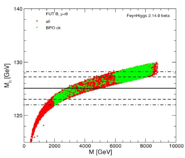
Figure 6.1: The lightest Higgs boson mass, $M_{h}$, as a function of $M$ for the choice $\mu<0$. The green points are the ones that satisfy the $B$-physics constraints. Taken from Ref. [195].

The allowed values of the lightest Higgs boson mass limit the allowed supersymmetric masses’ values, as shown in Fig. 6.2 [195]. In the left (right) plot we impose $M_{h}=125.1\pm 3.1~{}(2.1)~{}{\rm GeV}$. In particular, very heavy coloured SUSY particles are favoured (nearly independent of the $M_{h}$ uncertainty), in agreement with the non-observation of those particles at the LHC [197]. The only part that can be tested at the (HL-)LHC is the lower range of the neutral Higgs spectrum. For the $\tan\beta$ values favoured by our analysis, values up to $2\,\,\mathrm{TeV}$ are projected to be in the range of the ATLAS/CMS searches via $pp\to H/A\to\tau^{+}\tau^{-}$ [198], which would cover the lower part of the spectrum. On the other hand, the allowed coloured supersymmetric masses will remain unobservable at the (HL-)LHC, the ILC or CLIC. The lower part of the electroweak spectrum could be accessible at CLIC with $\sqrt{s}=3\,\,\mathrm{TeV}$ The coloured spectrum would be accessible, however, at the FCC-hh [199], as would be the full heavy Higgs spectrum.

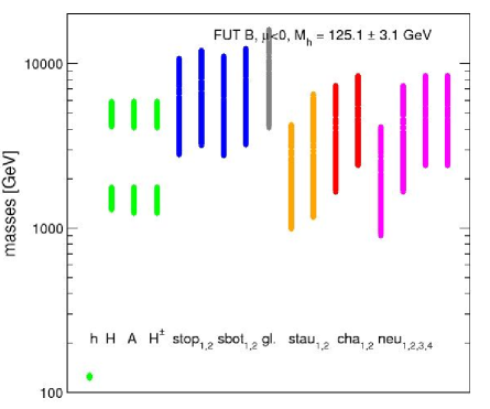
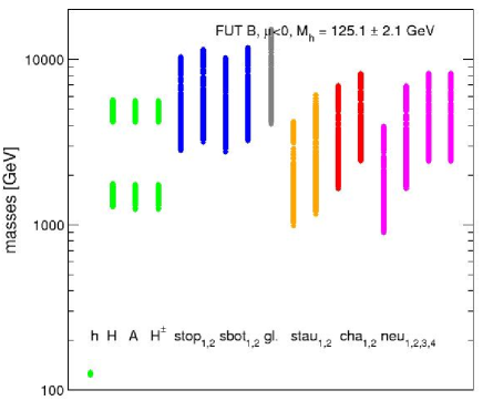
Figure 6.2: The (left,right) plots show the spectrum of the FUT model after imposing the constraint $M_{h}=125.1\pm 3.1(2.1)~{}{\rm GeV}$. The light (green) points are the various Higgs boson masses; the dark (blue) points following are the two scalar top and bottom masses; the gray ones are the gluino masses; then come the scalar tau masses in orange (light gray); the darker (red) points to the right are the two chargino masses; followed by the lighter shaded (pink) points indicating the neutralino masses. Taken from Ref. [195].

In Tab. 6.1 two example spectra of FUT are shown, which span the mass range of the parameter space that is in agreement with the $B$-physics observables and the lightest Higgs boson mass measurement. We show the lightest and the heaviest spectrum (based on $m_{\tilde{\chi}_{1}^{0}}$) for $\delta M_{h}=2.1$ and $\delta M_{h}=3.1$. The Higgs boson masses are denoted as $M_{h}$, $M_{H}$, $M_{A}$ and $M_{H^{\pm}}$. $m_{\tilde{t}_{1,2}}$, $m_{\tilde{t}_{1,2}}$, $m_{\tilde{g}}$ and $m_{\tilde{\tau}_{1,2}}$, are the scalar top, bottom, gluino and tau masses, respectively. $m_{\tilde{\chi}_{1,2}^{\pm}}$ and $m_{\tilde{\chi}_{1,2,3,4}^{0}}$ stand for chargino and neutralino masses, respectively. As discussed above, only the neutral Higgs spectrum of the “light spectrum” is in the range of the (HL-)LHC. Scalar taus as well as the two lighter neutralinos would be accessible at CLIC. For the “heavy spectrum” only the FCC-hh could test it.

$\delta M_{h}=2.1$	$M_{h}$	$M_{H}$	$M_{A}$	$M_{H^{\pm}}$	$m_{\tilde{t}_{1}}$	$m_{\tilde{t}_{2}}$	$m_{\tilde{b}_{1}}$	$m_{\tilde{b}_{2}}$	$m_{\tilde{g}}$
lightest	123.1	1533	1528	1527	2800	3161	2745	3219	4077
heaviest	127.2	4765	4737	4726	10328	11569	10243	11808	15268
	$m_{\tilde{\tau}_{1}}$	$m_{\tilde{\tau}_{2}}$	$m_{\tilde{\chi}_{1}^{\pm}}$	$m_{\tilde{\chi}_{2}^{\pm}}$	$m_{\tilde{\chi}_{1}^{0}}$	$m_{\tilde{\chi}_{2}^{0}}$	$m_{\tilde{\chi}_{3}^{0}}$	$m_{\tilde{\chi}_{4}^{0}}$	$\tan\beta$
lightest	983	1163	1650	2414	900	1650	2410	2414	45
heaviest	4070	5141	6927	8237	3920	6927	8235	8237	46

$\delta M_{h}=3.1$	$M_{h}$	$M_{H}$	$M_{A}$	$M_{H^{\pm}}$	$m_{\tilde{t}_{1}}$	$m_{\tilde{t}_{2}}$	$m_{\tilde{b}_{1}}$	$m_{\tilde{b}_{2}}$	$m_{\tilde{g}}$
lightest	122.8	1497	1491	1490	2795	3153	2747	3211	4070
heaviest	127.9	4147	4113	4103	10734	12049	11077	12296	16046
	$m_{\tilde{\tau}_{1}}$	$m_{\tilde{\tau}_{2}}$	$m_{\tilde{\chi}_{1}^{\pm}}$	$m_{\tilde{\chi}_{2}^{\pm}}$	$m_{\tilde{\chi}_{1}^{0}}$	$m_{\tilde{\chi}_{2}^{0}}$	$m_{\tilde{\chi}_{3}^{0}}$	$m_{\tilde{\chi}_{4}^{0}}$	$\tan\beta$
lightest	1001	1172	1647	2399	899	647	2395	2399	44
heaviest	4039	6085	7300	8409	4136	7300	8406	8409	45

Table 6.1: Two example spectra of the FUT . All masses are in GeV and rounded to 1 (0.1) GeV (for the light Higgs mass).

6.2.2 FUT Conclusions

One can see that the predictions of FUT are impressive. But one could also add some comments on the theoretical side. The developments on treating the problem of divergencies include string and non-commutative theories, as well as $N=4$ supersymmetric theories [79, 200], $N=8$ supergravity [201, 202, 203, 204, 205] and the AdS/CFT correspondence [206]. It is interesting that the $N=1$ FUT discussed here includes ideas that have survived phenomenological and theoretical tests, as well as the ultraviolet divergence problem and solves it in a minimal way.

In our analysis of FUT [195] we included restrictions of third generation quark masses and $B$-physics observables and it proved consistent with all the phenomenological constraints. Compared to our previous analyses [208, 120, 207, 196, 119, 209], the improved evaluation of $M_{h}$ prefers a heavier (Higgs) spectrum and thus allows only a heavy supersymmetric spectrum. The coloured spectrum easily escapes (HL-)LHC searches, but can likely be tested at the FCC-hh. However, the lower part of the EW spectrum could be observable at CLIC.

6.3 Numerical Analysis of the Reduced MSSM

In this section we analyze the particle spectrum predicted by the reduced MSSM [210]. We first discuss the selection of free parameters, then apply constraints from fermion masses. Subsequently we apply the remaining constraints and discuss the observability at current and future colliders.

6.3.1 Free Parameters of the Reduced MSSM

So far the relations among reduced parameters in terms of the fundamental ones derived in Sect. 5.5 had a part which was RGI and a another part originating from the corrections, which are scale dependent. In the analysis shown here we choose the unification scale to apply the corrections to the RGI relations. It should be noted that we are assuming a covering GUT, and thus unification of the three gauge couplings, as well as a unified gaugino mass $M$ at that scale. Also to be noted is that in the dimensionless sector of the theory, since $Y_{\tau}$ cannot be reduced in favour of the fundamental parameter $\alpha_{3}$, the mass of the $\tau$ lepton is an input parameter and consequently $\rho_{\tau}$, is an independent parameter too. At low energies, we fix the values of $\rho_{\tau}$ and $\tan\beta$ using the mass of the tau lepton $m_{\tau}(M_{Z})=1.7462$ GeV. For each value of $\rho_{\tau}$ there is a corresponding value of $\tan\beta$ that gives the appropriate $m_{\tau}(M_{Z})$. Then we use the value found for $\tan\beta$ together with $G_{t,b}$, as obtained from the reduction equations and their respective corrections, to determine the top and bottom quark masses. We require that both the bottom and top masses are within 2$\sigma$ of their experimental value, which singles out large $\tan\beta$ values, $\tan\beta\sim 42-47$. Correspondingly, in the dimensionful sector of the theory the $\rho_{h_{\tau}}$ is a free parameter, since $h_{\tau}$ cannot be reduced in favour of the fundamental parameter $M$ (the unified gaugino mass scale). $\mu$ is a free parameter, as it cannot be reduced in favour of $M_{3}$ as discussed above. On the other hand $m_{3}^{2}$ could be reduced, but here it is chosen to leave it free. However, $\mu$ and $m_{3}^{2}$ are restricted from the requirement of EWSB, and only $\mu$ is taken as an independent parameter. Finally, the other parameter in the Higgs-boson sector, the ${{\cal CP}}$-odd Higgs-boson mass $M_{A}$ is evaluated from $\mu$, as well as from $m_{H_{u}}^{2}$ and $m_{H_{d}}^{2}$, which are obtained from the reduction equations. In total we vary the parameters $\rho_{\tau}$, $\rho_{h_{\tau}}$, $M$ and $\mu$.

6.3.2 Constraints from Fermion Masses

The first step of the numerical analysis concerns the top and the bottom quark masses. As mentioned above, the variation of $\rho_{\tau}$ yields the values of $m_{t}$ (the top pole mass) and $m_{b}(M_{Z})$, the running bottom quark mass at the $Z$ boson mass scale, where scan points which are not within $2\sigma$ of the experimental data are neglected. This is shown in Fig. 6.3 [210]. The experimental values are indicated by the horizontal lines and are taken to be [171] (the same comments on the experimental values as in Sect. 5.1.3 apply)

$$m_{t}=173.34\pm 1.52\,\,\mathrm{GeV}~{},\quad m_{b}(M_{Z})=2.83\pm 0.1\,\,\mathrm{GeV}~{},$$ (6.8)

with the uncertainties at the $2\,\sigma$ level. One can see that the scan yields many parameter points that are in very good agreement with the experimental data. At the same time also the flavor constraints, see Sect. 6.1 are applied and shown as green dots. One can see that they are in good agreement with the measurements of the quark masses and give restrictions in the allowed ranges of $M$ (the common gaugino mass at the unification scale).

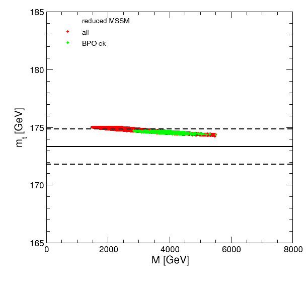
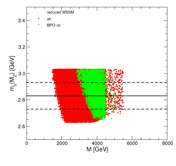
Figure 6.3: The left (right) plot shows our results within the reduced MSSM for the top (bottom) quark mass. The horizontal lines indicate the experimental values as given in Eq. (6.8). Taken from Ref. [210].

6.3.3 Predictions of the reduced MSSM for future colliders

As the next step the lightest MSSM Higgs-boson mass is evaluated. The prediction for $M_{h}$ is shown in Fig. 6.4 [210] as a function of $M$ in the range $1\,\,\mathrm{TeV}\;\raisebox{-3.00003pt}{$\stackrel{{\scriptstyle\displaystyle<}}{{\sim}}$}\;M\;\raisebox{-3.00003pt}{$\stackrel{{\scriptstyle\displaystyle<}}{{\sim}}$}\;6\,\,\mathrm{TeV}$. The lightest Higgs mass ranges in

$$M_{h}\sim 124-129\,\,\mathrm{GeV}~{},$$ (6.9)

where we discard the “spreaded” points with possibly lower masses, which result from a numerical instability in the Higgs-boson mass calculation. One should keep in mind that these predictions are subject to a theory uncertainty of $3(2)\,\,\mathrm{GeV}$, see Sect. 6.1. The red points correspond to the full parameter scan, whereas the green points are the subset that is in agreement with the $B$-physics observables as discussed above (which do not exhibit any numerical instability). The inclusion of the flavor observables shifts the lower bound for $M_{h}$ up to $\sim 126\,\,\mathrm{GeV}$.

The horizontal lines in Fig. 6.4 show the central value of the experimental measurement (solid), the $\pm 2.1\,\,\mathrm{GeV}$ uncertainty (dashed) and the $\pm 3.1\,\,\mathrm{GeV}$ uncertainty (dot-dashed). The requirement to obtain a light Higgs boson mass value in the correct range yields an upper limit on $M$ of about $5\,(4)\,\,\mathrm{TeV}$ for $M_{h}=125.1\pm 2.1\,(3.1)\,\,\mathrm{GeV}$.

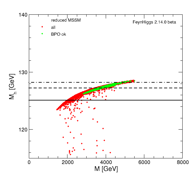
Figure 6.4: The lightest Higgs boson mass, $M_{h}$, as a function of $M$ (the common gaugino mass at the unification scale) in the reduced MSSM. The red points is the full model prediction. The green points fulfill the $B$-physics constraints (see text). Taken from Ref. [210].

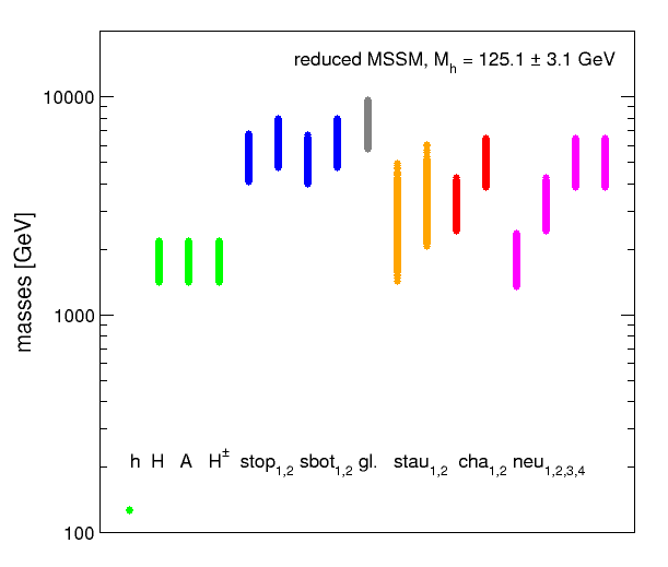
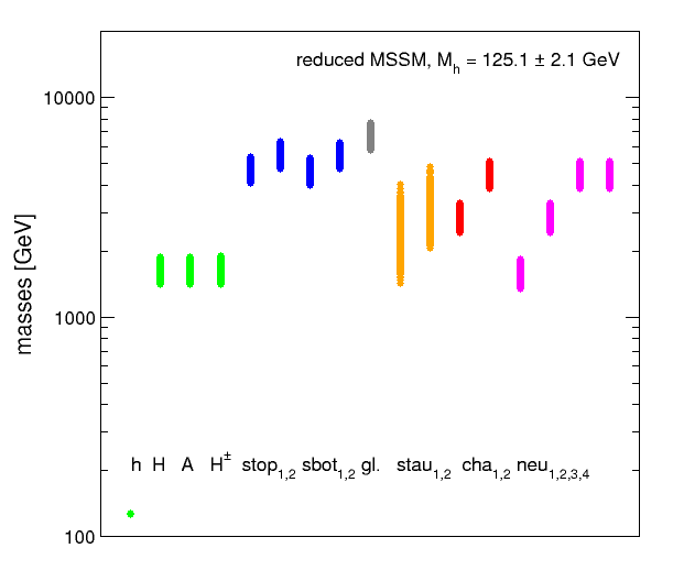
Figure 6.5: The left (right) plot shows the spectrum of the reduced MSSM after imposing the constraint $M_{h}=125.1\pm 3.1\,(2.1)\,\,\mathrm{GeV}$. The points shown are in agreement with the $B$-physics observables. The light (green) points on the left are the various Higgs boson masses. The dark (blue) points following are the two scalar top and bottom masses, followed by the lighter (gray) gluino mass. Next come the lighter (beige) scalar tau masses. The darker (red) points to the right are the two chargino masses followed by the lighter shaded (pink) points indicating the neutralino masses.

Naturally the $M_{h}$ limit also sets an upper limit on the low-energy SUSY masses. This turns the reduced MSSM into a highly predictive and testable theory. The full particle spectrum of the reduced MSSM (where we restricted ourselves as before to the third generation of sfermions) compliant with the $B$-physics observables is shown in Fig. 6.5 [210]. In the left (right) plot we impose $M_{h}=125.1\pm 3.1\,(2.1)\,\,\mathrm{GeV}$. Including the Higgs mass constraints in general favours the somewhat higher part of the SUSY particle mass spectra. The tighter $M_{h}$ range cuts off the very high SUSY mass scales.

The Higgs spectrum will be fully testable at the HL-LHC, which for $\tan\beta\;\raisebox{-3.00003pt}{$\stackrel{{\scriptstyle\displaystyle>}}{{\sim}}$}\;40$ can explore masses up to $\sim 2\,\,\mathrm{TeV}$ via the channel $pp\to H/A\to\tau^{+}\tau^{-}$ [198]. However, such observations would be in agreement also with a pure 2HDM, and additional observation of the SUSY particles will be necessary to analyze the model.

The lighter SUSY particles are given by the electroweak spectrum, which starts around $\sim 1.3\,\,\mathrm{TeV}$. They will mostly remain unobservable at the LHC and at future $e^{+}e^{-}$ colliders such as the ILC or CLIC, with only the very lower range mass range below $\sim 1.5\,\,\mathrm{TeV}$ might be observable at CLIC (with $\sqrt{s}=3\,\,\mathrm{TeV}$). The coloured mass spectrum starts at around $\sim 4\,\,\mathrm{TeV}$, which will remain unobservable at the (HL-)LHC. However, the coloured spectrum would be accessible at the FCC-hh [199]. This collider could definitely confirm the SUSY spectrum of the reduced MSSM or rule out this model.

	$M_{h}$	$M_{H}$	$M_{A}$	$M_{H^{\pm}}$	$m_{\tilde{t}_{1}}$	$m_{\tilde{t}_{2}}$	$m_{\tilde{b}_{1}}$	$m_{\tilde{b}_{2}}$	$m_{\tilde{g}}$
light	126.2	1433	1433	1446	4052	4736	3989	4723	5789
$\delta M_{h}=2.1$	127.2	1570	1570	1572	5361	6289	5282	6279	7699
$\delta M_{h}=3.1$	128.1	1886	1886	1888	6762	7951	6653	7943	9683

	$m_{\tilde{\tau}_{1}}$	$m_{\tilde{\tau}_{2}}$	$m_{\tilde{\chi}_{1}^{\pm}}$	$m_{\tilde{\chi}_{2}^{\pm}}$	$m_{\tilde{\chi}_{1}^{0}}$	$m_{\tilde{\chi}_{2}^{0}}$	$m_{\tilde{\chi}_{3}^{0}}$	$m_{\tilde{\chi}_{4}^{0}}$	$\tan\beta$
light	1906	2066	2430	3867	1339	2430	3864	3866	42.6
$\delta M_{h}=2.1$	1937	2531	3299	5166	1833	3299	5114	5116	43.1
$\delta M_{h}=3.1$	3153	3490	4248	6464	2376	4248	6462	6464	45.2

Table 6.2: Three example spectra of the reduced MSSM. “light” has the smallest $\tilde{\chi}_{1}^{0}$ in our sample, “$\delta M_{h}=2.1(3.1)$” has the largest $m_{\tilde{\chi}_{1}^{0}}$ for $M_{h}\leq 125.1+2.1(3.1)\,\,\mathrm{GeV}$. All masses are in GeV and rounded to 1 (0.1) GeV (for the light Higgs mass).

In Tab. 6.2 we show three example spectra of the reduced MSSM, which span the mass range of the parameter space that is in agreement with the $B$-physics observables and the Higgs-boson mass measurement (using the same notation as in Tab. 6.1). The rows labelled “light” correspond to the spectrum with the smallest $m_{\tilde{\chi}_{1}^{0}}$ value (which is independent of upper limit in $M_{h}$). This point is an example for the lowest $M_{h}$ values that we can reach in our scan. As discussed above, the heavy Higgs boson spectrum starts above $1.4\,\,\mathrm{TeV}$, which can be covered at the HL-LHC. The coloured spectrum is found between $\sim 4\,\,\mathrm{TeV}$ and $\sim 6\,\,\mathrm{TeV}$, outside the range of the (HL-)LHC. The LSP has a mass of $m_{\tilde{\chi}_{1}^{0}}=1339$, which might offer the possibility of $e^{+}e^{-}\to\tilde{\chi}_{1}^{0}\tilde{\chi}_{1}^{0}\gamma$ at CLIC. All other electroweak particles are too heavy to be produced at CLIC or the (HL-)LHC. “$\delta M_{h}=2.1(3.1)$” has the largest $m_{\tilde{\chi}_{1}^{0}}$ for $M_{h}\leq 125.1+2.1(3.1)\,\,\mathrm{GeV}$. While, following the mass relations in the reduced MSSM, the mass spectra are substantially heavier than in the “light” case, one can also observe that the smaller upper limit on $M_{h}$ results in substantially lower upper limits on the various SUSY and Higgs-boson masses. In both cases the heavy Higgs spectrum is within the reach of the HL-LHC, as mentioned above. However, even in the case of $\delta M_{h}=2.1\,\,\mathrm{GeV}$, all SUSY particles are outside the reach of the (HL-)LHC and CLIC. On the other hand, all spectra offer good possibilities for their discovery at the FCC-hh [199], as discussed above.

6.3.4 Conclusions about the Reduced MSSM

The reduced MSSM naturally results in a light Higgs boson in the mass range measured at the LHC. Only the Higgs sector can be tested at the HL-LHC. On the other hand, the rest of the SUSY spectrum will remain (likely) unaccessible at the (HL-)LHC, ILC and CLIC, where such a heavy spectrum also results in SM-like light Higgs boson, in agreement with LHC measurements [211]. In other words, the model is naturally in full agreement with all LHC measurements. It can be tested definitely at the FCC-hh, where large parts of the SUSY spectrum would be in the kinematic reach.

Chapter 7 Conclusions

In the present review we have presented in some detail the ideas concerning the reduction of independent parameters of various renormalizable theories, the theoretical tools which have been developed to attack the problem and the background work on which they are based on. Last but not least emphasis was given in presenting various models in which the reduction of parameters has been theoretically explored and confronted with the experimental data.

The reduction of couplings principle, expressed via RGI relations among couplings, provides us with a very interesting framework to search for more fundamental quantum field theories in which a group of couplings are related to a primary one, thus reducing substantially the number of free parameters of the theory, which might pave the way to search for the minimal ultimate one of Nature.

The reduction of couplings supplemented with global $N=1$ supersymmetry, leads to theories where the dimensionless gauge, Yukawa and the dimensionful supersymmetry breaking sectors are unified. An admirable success of this procedure is the construction of $N=1$ Finite Unified Theories, which solves probably the most basic problem of field theory, namely the problem of UV divergencies, in a minimal way.

On the phenomenological side, the developed reduction of couplings machinery provides us with strict selection rules in choosing realistic GUTs which lead to testable predictions. The celebrated success of predicting the top-quark mass in FUTs [18, 19, 20] was extended to the correct prediction of the Higgs boson mass, as well as a prediction for the supersymmetric spectrum of the MSSM [119, 121, 120, 207].

Furthermore it is possible to apply the reduction of couplings directly in the MSSM, again decreasing substantially the number of free parameters and making the model more predictive [150, 151, 195, 209, 210]. The two models selected by our analysis (FUT and reduced MSSM presented in Chapters 5 and 6) share similar features and are in natural agreement with all LHC measurements and searches. For the reduced MSSM the heavy Higgs particles will be accessible at the HL-LHC, while the supersymmetric particles will likely escape the detection at the (HL-)LHC, as well as at ILC and CLIC. In the FUT case parts of the allowed spectrum of the heavy Higgs bosons is accessible at the HL-LHC, and parts of the lighter scalar tau or the lighter neutralinos might be accessible at CLIC. On the other hand, the FCC-hh will be able to test the predicted parameter space for both models. The discovery of these particles is the next big bet on the phenomenological side. On the theoretical side the challenge is to develop a framework in which the above successes of the field theory models are combined with gravity.

Acknowledgments

We would like to thank a number of scientists from whom we have been introduced in the subject and others with whom we had an open dialogue and a constant encouragement to continue. Naturally we start by expressing our deepest gratitude to Wolfhart Zimmermann, who had agreed to be one of the authors of the present article and to whom is dedicated. During all these years we feel we have learned a lot from our collaborators Jisuke Kubo, Ernest Ma, Tatsuo Kobayashi and Dimitris Kapetanakis and we had the pleasure to exchange information and ideas on the subject with Reinhard Oehme, Raymond Stora, who unfortunately are not with us, while we are always enjoying and appreciate very much indeed the continuous exchange of ideas and the encouragement given to us by Geneviève Bélanger, Fawzi Boudjema, Cédric Delaunay, Abdelhak Djouadi, Thomas Hahn, Wolfgang Hollik, Luis Ibanez, Jan Kalinowski, Dmitry Kazakov, Kostas Kounnas, Dieter Lüst, Carlos Muñoz, Erhard Seiler, Klaus Sibold and Christof Wetterich.
The work of S.H. is supported in part by the MEINCOP Spain under Contract FPA2016-78022-P, in part by the Spanish Agencia Estatal de Investigación (AEI), the EU Fondo Europeo de Desarrollo Regional (FEDER) through the project FPA2016-78645-P, in part by the “Spanish Red Consolider MultiDark” FPA2017-90566-REDC, and in part by the AEI through the grant IFT Centro de Excelencia Severo Ochoa SEV-2016-0597. The work of M.M. is partly supported by UNAM PAPIIT through Grant IN111518. The work of N.T. and G.Z. is partially supported by the COST actions CA15108 and CA16201. One of us (GZ) has been supported within the Excellence Initiative funded by the German and State Governments, at the Institute for Theoretical Physics, Heidelberg University and from the Excellence Grant Enigmass of LAPTh. GZ thanks the ITP of Heidelberg, LAPTh of Annecy and MPI Munich for their hospitality.

Bibliography

- [1] J. Kubo, S. Heinemeyer, M. Mondragon, O. Piguet, K. Sibold, W. Zimmermann and G. Zoupanos, PoS (Higgs & top)001, Ed. Klaus Sibold, https://pos.sissa.it/cgi-bin/reader/conf.cgi?confid=222. A short version is published in arXiv:1411.7155 [hep-ph].
- [2] J. C. Pati and A. Salam, Phys. Rev. Lett. 31 (1973) 661.
- [3] H. Georgi and S. L. Glashow, Phys. Rev. Lett. 32 (1974) 438.
- [4] H. Georgi, H. R. Quinn and S. Weinberg, Phys. Rev. Lett. 33 (1974) 451.
- [5] H. Fritzsch and P. Minkowski, Annals Phys. 93 (1975) 193.
- [6] F. Gursey, P. Ramond and P. Sikivie, Phys. Lett. 60B (1976) 177.
- [7] Y. Achiman and B. Stech, Phys. Lett. 77B (1978) 389.
- [8] U. Amaldi, W. de Boer and H. Furstenau, Phys. Lett. B 260 (1991) 447.
- [9] S. Dimopoulos and H. Georgi, Nucl. Phys. B 193 (1981) 150.
- [10] N. Sakai, Z. Phys. C 11 (1981) 153.
- [11] A. J. Buras, J. R. Ellis, M. K. Gaillard and D. V. Nanopoulos, Nucl. Phys. B 135 (1978) 66.
- [12] W. Zimmermann, Commun. Math. Phys. 97 (1985) 211.
- [13] R. Oehme, W. Zimmermann, Commun. Math. Phys. 97 (1985) 569.
- [14] R. Oehme, Prog. Theor. Phys. Suppl. 86 (1986) 215.
- [15] E. Ma, Phys. Rev. D 17 (1978) 623; E. Ma, Phys. Rev. D 31 (1985) 1143.
- [16] N. P. Chang, Phys. Rev. D 10 (1974) 2706.
- [17] S. Nandi and W. C. Ng, Phys. Rev. D 20 (1979) 972.
- [18] D. Kapetanakis, M. Mondragón, G. Zoupanos, Z. Phys. C60 (1993) 181.
- [19] M. Mondragón, G. Zoupanos, Nucl. Phys. Proc. Suppl. 37C (1995) 98.
- [20] J. Kubo, M. Mondragón, G. Zoupanos, Nucl. Phys. B424 (1994) 291.
- [21] Tevatron Electroweak Working Group, CDF and D0 Collaborations, (2011), 1107.5255.
- [22] ATLAS Collaboration, G. Aad et al., Phys.Lett. B716 (2012) 1, 1207.7214;
- [23] ATLAS Collaboration, Reports ATLAS-CONF-2013-014, ATLAS-COM-CONF-2013-025 (2013).
- [24] CMS Collaboration, S. Chatrchyan et al., Phys.Lett. B716, 30 (2012), arXiv:1207.7235.
- [25] CMS Collaboration, S. Chatrchyan et al., (2013), arXiv:1303.4571.
- [26] J. Kubo, K. Sibold and W. Zimmermann, Nucl. Phys. B259, 331 (1985).
- [27] J. Kubo, K. Sibold and W. Zimmermann, Phys. Lett. B220, 185 (1989).
- [28] J. Wess and B. Zumino, Phys. Lett. 49B (1974) 52.
- [29] J. Iliopoulos and B. Zumino, Nucl. Phys. B 76 (1974) 310.
- [30] S. Ferrara, J. Iliopoulos and B. Zumino, Nucl. Phys. B 77 (1974) 413.
- [31] K. Fujikawa and W. Lang, Nucl. Phys. B 88 (1975) 61.
- [32] A. Parkes and P. C. West, Phys. Lett. 138B (1984) 99.
- [33] P. C. West, Phys. Lett. 137B (1984) 371.
- [34] D. R. T. Jones and A. J. Parkes, Phys. Lett. 160B (1985) 267.
- [35] D. R. T. Jones and L. Mezincescu, Phys. Lett. 138B (1984) 293.
- [36] A. J. Parkes, Phys. Lett. 156B (1985) 73.
- [37] R. Oehme, K. Sibold and W. Zimmermann, Phys. Lett. 147B (1984) 115.
- [38] T. P. Cheng, E. Eichten and L. F. Li, Phys. Rev. D 9 (1974) 2259.
- [39] W. Zimmermann, Phys. Lett. B 311 (1993) 249.
- [40] O. Piguet and K. Sibold, Phys. Lett. B 229 (1989) 83.
- [41] J. Kubo, M. Mondragón and G. Zoupanos, Phys. Lett. B 389 (1996) 523 [hep-ph/9609218].
- [42] P. Breitenlohner and D. Maison, Commun. Math. Phys. 219 (2001) 179.
- [43] W. Zimmermann, Commun. Math. Phys. 219 (2001) 221.
- [44] I. Jack, D. R. T. Jones, Phys. Lett. B349 (1995) 294.
- [45] Y. Kawamura, T. Kobayashi, J. Kubo, Phys. Lett. B405 (1997) 64.
- [46] T. Kobayashi, J. Kubo, M. Mondragón, G. Zoupanos, Nucl. Phys. B511 (1998) 45.
- [47] R. Delbourgo, Nuovo Cim. A 25 (1975) 646.
- [48] A. Salam and J. A. Strathdee, Nucl. Phys. B 86 (1975) 142.
- [49] M. T. Grisaru, W. Siegel and M. Rocek, Nucl. Phys. B 159 (1979) 429.
- [50] L. Girardello and M. T. Grisaru, Nucl. Phys. B 194 (1982) 65.
- [51] Y. Yamada, Phys. Rev. D 50 (1994) 3537 [hep-ph/9401241].
- [52] D. I. Kazakov, Phys. Lett. B 421 (1998) 211 [hep-ph/9709465].
- [53] I. Jack, D. R. T. Jones and A. Pickering, Phys. Lett. B 426 (1998) 73 [hep-ph/9712542].
- [54] J. Hisano and M. A. Shifman, Phys. Rev. D 56 (1997) 5475 [hep-ph/9705417].
- [55] I. Jack and D. R. T. Jones, Phys. Lett. B 415 (1997) 383 [hep-ph/9709364].
- [56] L. V. Avdeev, D. I. Kazakov and I. N. Kondrashuk, Nucl. Phys. B 510 (1998) 289 [hep-ph/9709397].
- [57] D. I. Kazakov, Phys. Lett. B 449 (1999) 201 [hep-ph/9812513].
- [58] V. A. Novikov, M. A. Shifman, A. I. Vainshtein, V. I. Zakharov, Nucl. Phys. B229 (1983) 407.
- [59] V. A. Novikov, M. A. Shifman, A. I. Vainshtein and V. I. Zakharov, Phys. Lett. 166B (1986) 329 [Sov. J. Nucl. Phys. 43 (1986) 294] [Yad. Fiz. 43 (1986) 459].
- [60] M. A. Shifman, Int. J. Mod. Phys. A 11 (1996) 5761 [hep-ph/9606281].
- [61] T. Kobayashi, J. Kubo, G. Zoupanos, Phys. Lett. B427 (1998) 291.
- [62] L. E. Ibanez, D. Lust, Nucl. Phys. B382 (1992) 305.
- [63] A. Brignole, L. E. Ibanez, C. Munoz and C. Scheich, Z. Phys. C 74 (1997) 157 [hep-ph/9508258].
- [64] I. Jack and D. R. T. Jones, Phys. Lett. B 465 (1999) 148 [hep-ph/9907255].
- [65] T. Kobayashi et al., AIP Conf. Proc. 490 (1999) 279.
- [66] A. Karch, T. Kobayashi, J. Kubo and G. Zoupanos, Phys. Lett. B 441 (1998) 235 [hep-th/9808178].
- [67] L. Randall and R. Sundrum, Nucl. Phys. B 557 (1999) 79 [hep-th/9810155].
- [68] G. F. Giudice, M. A. Luty, H. Murayama and R. Rattazzi, JHEP 9812 (1998) 027 [hep-ph/9810442].
- [69] T. Gherghetta, G. F. Giudice and J. D. Wells, Nucl. Phys. B 559 (1999) 27 [hep-ph/9904378].
- [70] A. Pomarol and R. Rattazzi, JHEP 9905 (1999) 013 [hep-ph/9903448].
- [71] Z. Chacko, M. A. Luty, I. Maksymyk and E. Ponton, JHEP 0004 (2000) 001 [hep-ph/9905390].
- [72] E. Katz, Y. Shadmi and Y. Shirman, JHEP 9908 (1999) 015 [hep-ph/9906296].
- [73] R. Hodgson, I. Jack, D. R. T. Jones and G. G. Ross, Nucl. Phys. B 728 (2005) 192 [hep-ph/0507193].
- [74] S. Heinemeyer, J. Kubo, M. Mondragón, O. Piguet, K. Sibold, W. Zimmermann and G. Zoupanos, arXiv:1411.7155 [hep-ph].
- [75] W. Hollik, CERN Yellow Report CERN-2010-002, 1-44 [arXiv:1012.3883 [hep-ph]].
- [76] J. Kubo, Phys. Lett. B 262 (1991) 472.
- [77] S. Kachru and E. Silverstein, Phys. Rev. Lett. 80 (1998) 4855, hep-th/9802183.
- [78] M. F. Sohnius and P. C. West, Phys. Lett. 100B (1981) 245.
- [79] S. Mandelstam, Nucl. Phys. B 213 (1983) 149.
- [80] L. Brink, O. Lindgren and B. E. W. Nilsson, Nucl. Phys. B 212, 401 (1983).
- [81] P. L. White, Class. Quant. Grav. 9 (1992) 413.
- [82] A. Chatzistavrakidis, H. Steinacker and G. Zoupanos, JHEP 1005 (2010) 100, 1002.2606.
- [83] P. S. Howe, K. S. Stelle and P. C. West, Phys. Lett. 124B (1983) 55.
- [84] P. S. Howe, K. S. Stelle and P. K. Townsend, Nucl. Phys. B 236 (1984) 125.
- [85] P. C. West, Conf. Proc. C 8306011 (1983) 127.
- [86] S. Rajpoot and J. G. Taylor, Phys. Lett. B147, 91 (1984).
- [87] S. Rajpoot and J. G. Taylor, Int. J. Theor. Phys. 25, 117 (1986).
- [88] D. R. T. Jones, L. Mezincescu, Y. P. Yao, Phys. Lett. B148 (1984) 317.
- [89] I. Jack, D. R. T. Jones, Phys. Lett. B333 (1994) 372.
- [90] L. O’Raifeartaigh, Nucl. Phys. B96, 331 (1975).
- [91] P. Fayet and J. Iliopoulos, Phys. Lett. B51, 461 (1974).
- [92] C. Lucchesi, O. Piguet, K. Sibold, Phys. Lett. B201 (1988) 241.
- [93] C. Lucchesi, O. Piguet, K. Sibold, Helv. Phys. Acta 61 (1988) 321.
- [94] S. Ferrara and B. Zumino, Nucl. Phys. B87, 207 (1975).
- [95] O. Piguet and K. Sibold, Nucl. Phys. B196, 428 (1982).
- [96] O. Piguet and K. Sibold, Nucl. Phys. B196, 447 (1982).
- [97] O. Piguet and K. Sibold, Int. J. Mod. Phys. A1, 913 (1986).
- [98] O. Piguet and K. Sibold, Phys. Lett. B177, 373 (1986).
- [99] P. Ensign and K. T. Mahanthappa, Phys. Rev. D36, 3148 (1987).
- [100] C. Lucchesi, G. Zoupanos, Fortschr. Phys. 45 (1997) 129.
- [101] O. Piguet, hep-th/9606045, talk given at “10th International Conference on Problems of Quantum Field Theory”.
- [102] L. Alvarez-Gaume and P. H. Ginsparg, Nucl. Phys. B243, 449 (1984).
- [103] W. A. Bardeen and B. Zumino, Nucl. Phys. B244, 421 (1984).
- [104] B. Zumino, Y.-S. Wu and A. Zee, Nucl. Phys. B239, 477 (1984).
- [105] A. V. Ermushev, D. I. Kazakov and O. V. Tarasov, Nucl. Phys. B 281 (1987) 72.
- [106] D. I. Kazakov, Mod. Phys. Lett. A 2 (1987) 663.
- [107] D. R. T. Jones, Nucl. Phys. B 277 (1986) 153.
- [108] D. I. Kazakov, M. Y. Kalmykov, I. N. Kondrashuk and A. V. Gladyshev, Nucl. Phys. B 471 (1996) 389
- [109] D. I. Kazakov, M. Y. Kalmykov, I. N. Kondrashuk and A. V. Gladyshev, Nucl. Phys. B 471 (1996) 389
- [110] R. G. Leigh and M. J. Strassler, Nucl. Phys. B447, 95 (1995), [hep-th/9503121].
- [111] D. I. Kazakov, Phys. Lett. B 421 (1998) 211
- [112] S. Hamidi, J. Patera and J. H. Schwarz, Phys. Lett. B141, 349 (1984).
- [113] D. R. T. Jones and S. Raby, Phys. Lett. B143, 137 (1984).
- [114] J. Leon, J. Perez-Mercader, M. Quiros and J. Ramirez-Mittelbrunn, Phys. Lett. B156, 66 (1985).
- [115] S. Hamidi and J. H. Schwarz, Phys. Lett. B147, 301 (1984).
- [116] K. S. Babu, T. Enkhbat and I. Gogoladze, Phys. Lett. B555, 238 (2003), [hep-ph/0204246].
- [117] T. Kobayashi, J. Kubo, M. Mondragón, G. Zoupanos, Acta Phys. Polon. B30 (1999) 2013.
- [118] M. Mondragón and G. Zoupanos, Acta Phys. Polon. B34, 5459 (2003).
- [119] S. Heinemeyer, M. Mondragón and G. Zoupanos, Phys. Part. Nucl. 44 (2013) 299.
- [120] S. Heinemeyer, M. Mondragón and G. Zoupanos, Phys. Lett. B 718 (2013) 1430 [arXiv:1211.3765 [hep-ph]].
- [121] S. Heinemeyer, M. Mondragón and G. Zoupanos, JHEP 0807 (2008) 135 [arXiv:0712.3630 [hep-ph]].
- [122] M. S. Carena, D. Garcia, U. Nierste and C. E. M. Wagner, Nucl. Phys. B577, 88 (2000), [hep-ph/9912516].
- [123] K. Nakamura et al. [Particle Data Group], J. Phys. G 37 (2010) 075021.
- [124] T. Kobayashi, J. Kubo, M. Mondragón and G. Zoupanos, Surveys High Energ. Phys. 16, 87 (2001).
- [125] J. Kubo, M. Mondragón, G. Zoupanos, Acta Phys. Polon. B27 (1997) 3911–3944.
- [126] S. Dimopoulos and H. Georgi, Nucl. Phys. B193 (1981) 150.
- [127] N. Sakai, Zeit. f. Phys. C11 (1981) 153.
- [128] J. Kubo, M. Mondragón and G. Zoupanos, Nucl. Phys. B424 (1994) 291.
- [129] N. Polonsky and A. Pomarol, Phys. Rev. Lett. 73 (1994) 2292.
- [130] J. Kubo, M. Mondragón, M. Olechowski and G. Zoupanos, Nucl. Phys. B 479 (1996) 25 [hep-ph/9512435].
- [131] J. Kubo, M. Mondragón, N. D. Tracas, G. Zoupanos, Phys. Lett. B342 (1995) 155.
- [132] J.C. Pati and A. Salam, Phys. Rev. Lett. 31 (1973) 661.
- [133] I. Antoniadis and G.K. Leontaris, Phys. Lett. B216 (1989) 333.
- [134] G. Leontaris and N. Tracas, Z. Phys. C56 (1992) 479; Phys. Lett. B291 (1992) 44.
- [135] H. Georgi and C. Jarlskog, Phys. Lett. B86 (1979) 297.
- [136] J. Kubo, M. Mondragón, S. Shoda, G. Zoupanos, Nucl. Phys. B469 (1996) 3.
- [137] H. Fritzsch and P. Minkowski, Ann. Phys. 93 (1975) 193.
- [138] H. Georgi, in Particles and Fields – 1974, ed. C.E. Carlson, (American Institute of Physics, New York).
- [139] R. N. Mohapatra, Proc. of a NATO ASI on Quarks, Leptons, and Beyond, September 5-16, 1983, Munich, eds. H. Fritsch et al. (Plenum Press, New York, 1983).
- [140] M. Tanabashi et al. [Particle Data Group], Phys. Rev. D 98 (2018) no.3, 030001.
- [141] E. Ma, M. Mondragón, and G. Zoupanos, JHEP 12, 026 (2004), hep-ph/0407236.
- [142] A. De Rújula, H. Georgi, and G. S. L., p. 88 (1984), Fifth Workshop on Grand Unification, K. Kang, H. Fried, and P. Frampton eds., World Scientific, Singapore.
- [143] G. Lazarides, C. Panagiotakopoulos, and Q. Shafi, Phys. Lett. B315, 325 (1993), hep-ph/9306332.
- [144] G. Lazarides and C. Panagiotakopoulos, Phys. Lett. B336, 190 (1994), hep-ph/9403317.
- [145] E. Ma, Phys. Rev. D36, 274 (1987).
- [146] N. Irges and G. Zoupanos, Phys. Lett. B 698 (2011) 146
- [147] N. Irges, G. Orfanidis and G. Zoupanos, PoS CORFU 2011 (2011) 105
- [148] M. Mondragon and G. Zoupanos, Phys. Part. Nucl. Lett. 8 (2011) 173.
- [149] Particle Data Group, C. Amsler et al., Phys. Lett. B667, 1 (2008).
- [150] M. Mondragón, N. D. Tracas and G. Zoupanos, Phys. Lett. B 728 (2014) 51 [arXiv:1309.0996 [hep-ph]].
- [151] M. Mondragón, S. Heinemeyer, N. Tracas and G. Zoupanos, PoS CORFU2016 (2017) 041.
- [152] M. Mondragón, N.D. Tracas, G. Zoupanos, Phys. Lett. B 728, 51 (2014).
- [153] P. Fayet, Nucl. Phys. B 149 (1979) 137.
- [154] R. Decker and J. Pestieau, Lett. Nuovo Cim. 29 (1980) 560.
- [155] M. J. G. Veltman, Acta Phys. Polon. B 12 (1981) 437.
- [156] B. Pendleton and G. G. Ross, Phys. Lett. 98B (1981) 291.
- [157] W. Zimmermann, Phys. Lett. B 308 (1993) 117. doi:10.1016/0370-2693(93)90611-K
- [158] C. T. Hill, Phys. Rev. D 24 (1981) 691.
- [159] W. A. Bardeen, C. T. Hill and M. Lindner, Phys. Rev. D 41 (1990) 1647.
- [160] W. A. Bardeen, M. Carena, S. Pokorski and C. E. M. Wagner, Phys. Lett. B 320 (1994) 110 [hep-ph/9309293].
- [161] S. Heinemeyer, O. Stal and G. Weiglein, Phys.Lett. B710 (2012) 201, 1112.3026.
- [162] B. Capdevila, A. Crivellin, S. Descotes-Genon, J. Matias and J. Virto, JHEP 1801 (2018) 093 [arXiv:1704.05340 [hep-ph]].
-
[163]
M. Misiak et al.,
Phys. Rev. Lett. 98 (2007) 022002
[hep-ph/0609232];
M. Ciuchini, G. Degrassi, P. Gambino and G. F. Giudice, Nucl. Phys. B 534 (1998) 3 [hep-ph/9806308];
G. Degrassi, P. Gambino and G. F. Giudice, JHEP 0012 (2000) 009 [hep-ph/0009337];
M. Carena, D. Garcia, U. Nierste and C. E. M. Wagner, Phys. Lett. B 499 (2001) 141 [hep-ph/0010003];
G. D’Ambrosio, G. F. Giudice, G. Isidori and A. Strumia, Nucl. Phys. B 645 (2002) 155 [hep-ph/0207036]. - [164] D. Asner et al. [Heavy Flavor Averaging Group], arXiv:1010.1589 [hep-ex].
- [165] R. Aaij et al. [LHCb Collaboration], Phys. Rev. Lett. 110 (2013) 021801 [arXiv:1211.2674 [Unknown]].
-
[166]
C. Bobeth, M. Gorbahn, T. Hermann, M. Misiak, E. Stamou and M. Steinhauser,
Phys. Rev. Lett. 112 (2014) 101801
[arXiv:1311.0903 [hep-ph]];
T. Hermann, M. Misiak and M. Steinhauser, JHEP 1312 (2013) 097 [arXiv:1311.1347 [hep-ph]];
C. Bobeth, M. Gorbahn and E. Stamou, Phys. Rev. D 89 (2014) no.3, 034023 [arXiv:1311.1348 [hep-ph]]. - [167] A. J. Buras, Phys. Lett. B 566 (2003) 115 [hep-ph/0303060]; G. Isidori and D. M. Straub, Eur. Phys. J. C 72 (2012) 2103 [arXiv:1202.0464 [hep-ph]].
- [168] S. Chatrchyan et al. [CMS Collaboration], Phys. Rev. Lett. 111 (2013) 101804 [arXiv:1307.5025 [hep-ex]].
- [169] CMS and LHCb Collaborations [CMS and LHCb Collaborations], CMS-PAS-BPH-13-007, LHCb-CONF-2013-012, CERN-LHCb-CONF-2013-012.
- [170] G. Isidori and P. Paradisi, Phys. Lett. B 639 (2006) 499 [hep-ph/0605012]; G. Isidori, F. Mescia, P. Paradisi and D. Temes, Phys. Rev. D 75 (2007) 115019 [hep-ph/0703035 [HEP-PH]].
- [171] K. A. Olive et al. [Particle Data Group], Chin. Phys. C 38 (2014) 090001.
- [172] A. J. Buras, P. Gambino, M. Gorbahn, S. Jager and L. Silvestrini, Nucl. Phys. B 592 (2001) 55 [hep-ph/0007313].
- [173] R. Aaij et al. [LHCb Collaboration], New J. Phys. 15 (2013) 053021 [arXiv:1304.4741 [hep-ex]].
- [174] S. Heinemeyer, Int. J. Mod. Phys. A 21 (2006) 2659 [hep-ph/0407244].
- [175] S. Heinemeyer, W. Hollik and G. Weiglein, Phys. Rept. 425 (2006) 265 [hep-ph/0412214].
- [176] A. Djouadi, Phys. Rept. 459 (2008) 1 [hep-ph/0503173].
- [177] S. Chatrchyan et al. [CMS Collaboration], Phys. Lett. B 716 (2012) 30 [arXiv:1207.7235 [hep-ex]].
- [178] S. Heinemeyer, O. Stal and G. Weiglein, Phys. Lett. B 710 (2012) 201 [arXiv:1112.3026 [hep-ph]].
- [179] P. Bechtle, S. Heinemeyer, O. Stal, T. Stefaniak, G. Weiglein and L. Zeune, Eur. Phys. J. C 73 (2013) no.4, 2354 [arXiv:1211.1955 [hep-ph]].
- [180] P. Bechtle, H. E. Haber, S. Heinemeyer, O. Stal, T. Stefaniak, G. Weiglein and L. Zeune, Eur. Phys. J. C 77 (2017) no.2, 67 [arXiv:1608.00638 [hep-ph]].
- [181] G. Aad et al. [ATLAS and CMS Collaborations], Phys. Rev. Lett. 114 (2015) 191803 [arXiv:1503.07589 [hep-ex]].
- [182] G. Degrassi, S. Heinemeyer, W. Hollik, P. Slavich and G. Weiglein, Eur. Phys. J. C28, 133 (2003), [hep-ph/0212020].
- [183] O. Buchmueller et al., Eur. Phys. J. C 74 (2014) no.3, 2809 [arXiv:1312.5233 [hep-ph]].
- [184] H. Bahl, S. Heinemeyer, W. Hollik and G. Weiglein, Eur. Phys. J. C 78 (2018) no.1, 57 [arXiv:1706.00346 [hep-ph]].
-
[185]
S. Heinemeyer, W. Hollik and G. Weiglein,
Comput. Phys. Commun. 124 (2000) 76
[hep-ph/9812320];
S. Heinemeyer, W. Hollik and G. Weiglein, Eur. Phys. J. C 9 (1999) 343 [hep-ph/9812472];
M. Frank, T. Hahn, S. Heinemeyer, W. Hollik, H. Rzehak and G. Weiglein, JHEP 0702 (2007) 047 [hep-ph/0611326];
T. Hahn, S. Heinemeyer, W. Hollik, H. Rzehak and G. Weiglein, Comput. Phys. Commun. 180 (2009) 1426.
T. Hahn, S. Heinemeyer, W. Hollik, H. Rzehak and G. Weiglein, Phys. Rev. Lett. 112 (2014) no.14, 141801 [arXiv:1312.4937 [hep-ph]];
H. Bahl and W. Hollik, Eur. Phys. J. C 76 (2016) no.9, 499 [arXiv:1608.01880 [hep-ph]];
H. Bahl, T. Hahn, S. Heinemeyer, W. Hollik, S. Paßehr, H. Rzehak and G. Weiglein, arXiv:1811.09073 [hep-ph];
See http://www.feynhiggs.de. -
[186]
H. Goldberg,
Phys. Rev. Lett. 50 (1983) 1419;
J. Ellis, J. Hagelin, D. Nanopoulos, K. Olive and M. Srednicki, Nucl. Phys. B 238 (1984) 453. -
[187]
E. Komatsu et al. [WMAP Collaboration],
Astrophys. J. Suppl. 192 (2011) 18
[arXiv:1001.4538 [astro-ph.CO]];
http://lambda.gsfc.nasa.gov/product/map/current/parameters.cfm. - [188] E. Komatsu et al. [WMAP Science Team], PTEP 2014 (2014) 06B102 [arXiv:1404.5415 [astro-ph.CO]].
-
[189]
M. Diaz, J. Romao and J. Valle,
Nucl. Phys. B 524 (1998) 23
[arXiv:hep-ph/9706315];
J. Valle, PoS corfu 98 (1998) 010 arXiv:hep-ph/9907222 and references therein;
M. Diaz, M. Hirsch, W. Porod, J. Romao and J. Valle, Phys. Rev. D 68 (2003) 013009 [Erratum-ibid. D 71 (2005) 059904] [arXiv:hep-ph/0302021]. -
[190]
H. K. Dreiner,
Adv. Ser. Direct. High Energy Phys. 21 (2010) 565
[hep-ph/9707435].
G. Bhattacharyya, In “Tegernsee 1997, Beyond the desert 1997” 194-201 [hep-ph/9709395].
B. Allanach, A. Dedes and H. Dreiner, Phys. Rev. D 60 (1999) 075014 [arXiv:hep-ph/9906209];
J. Romao and J. Valle, Nucl. Phys. B 381 (1992) 87; - [191] G. Bennett et al. [The Muon g-2 Collaboration], Phys. Rev. Lett. 92, 161802 (2004), [arXiv:hep-ex/0401008]; and Phys. Rev. D 73, 072003 (2006) [arXiv:hep-ex/0602035].
-
[192]
D. Stockinger,
J. Phys. G 34 (2007) R45
[hep-ph/0609168].
J. P. Miller, E. de Rafael and B. L. Roberts, Rept. Prog. Phys. 70 (2007) 795 [hep-ph/0703049].
J. Prades, E. de Rafael and A. Vainshtein, Adv. Ser. Direct. High Energy Phys. 20 (2009) 303 [arXiv:0901.0306 [hep-ph]].
F. Jegerlehner and A. Nyffeler, Phys. Rept. 477 (2009) 1 [arXiv:0902.3360 [hep-ph]].
M. Davier, A. Hoecker, B. Malaescu, C. Z. Yuan and Z. Zhang, Eur. Phys. J. C 66 (2010) 1 [arXiv:0908.4300 [hep-ph]].
J. Prades, Acta Phys. Polon. Supp. 3 (2010) 75 [arXiv:0909.2546 [hep-ph]].
T. Teubner, K. Hagiwara, R. Liao, A. D. Martin and D. Nomura, Chin. Phys. C 34 (2010) 728 [arXiv:1001.5401 [hep-ph]].
M. Davier, A. Hoecker, B. Malaescu and Z. Zhang, Eur. Phys. J. C 71 (2011) 1515 Erratum: [Eur. Phys. J. C 72 (2012) 1874] [arXiv:1010.4180 [hep-ph]]. - [193] F. Jegerlehner and R. Szafron, Eur. Phys. J. C 71 (2011) 1632 [arXiv:1101.2872 [hep-ph]].
- [194] M. Benayoun, P. David, L. DelBuono and F. Jegerlehner, Eur. Phys. J. C 73 (2013) 2453 [arXiv:1210.7184 [hep-ph]].
- [195] S. Heinemeyer, M. Mondragón, G. Patellis, N. Tracas and G. Zoupanos, Symmetry 10 (2018) no.3, 62 [arXiv:1802.04666 [hep-ph]].
- [196] S. Heinemeyer, M. Mondragón and G. Zoupanos, Int. J. Mod. Phys. Conf. Ser. 13 (2012) 118.
- [197] https://twiki.cern.ch/twiki/bin/view/AtlasPublic/SupersymmetryPublicResults, https://twiki.cern.ch/twiki/bin/view/CMSPublic/PhysicsResultsSUS
- [198] CMS Collaboration, CMS-DP-2016-064.
- [199] M. Mangano, CERN Yellow Report CERN 2017-003-M [arXiv:1710.06353 [hep-ph]].
- [200] L. Brink, O. Lindgren and B. E. W. Nilsson, Phys. Lett. 123B (1983) 323.
- [201] Z. Bern, J. J. Carrasco, L. J. Dixon, H. Johansson and R. Roiban, Phys. Rev. Lett. 103 (2009) 081301 [arXiv:0905.2326 [hep-th]].
- [202] R. Kallosh, JHEP 0909 (2009) 116 [arXiv:0906.3495 [hep-th]].
- [203] Z. Bern, J. J. Carrasco, L. J. Dixon, H. Johansson, D. A. Kosower and R. Roiban, Phys. Rev. Lett. 98 (2007) 161303 [hep-th/0702112].
- [204] Z. Bern, L. J. Dixon and R. Roiban, Phys. Lett. B 644 (2007) 265 [hep-th/0611086].
- [205] M. B. Green, J. G. Russo and P. Vanhove, Phys. Rev. Lett. 98 (2007) 131602 [hep-th/0611273].
- [206] J. M. Maldacena, Int. J. Theor. Phys. 38 (1999) 1113 [Adv. Theor. Math. Phys. 2 (1998) 231] [hep-th/9711200].
- [207] S. Heinemeyer, M. Mondragón and G. Zoupanos, Fortsch. Phys. 61 (2013) no.11, 969 [arXiv:1305.5073 [hep-ph]].
- [208] S. Heinemeyer, M. Mondragón and G. Zoupanos, SIGMA 6 (2010) 049 [arXiv:1001.0428 [hep-ph]].
- [209] S. Heinemeyer, M. Mondragón, N. Tracas and G. Zoupanos, Nucl. Phys. B 927 (2018) 319.
- [210] S. Heinemeyer, M. Mondragón, N. Tracas and G. Zoupanos, JHEP 1808 (2018) 150.
- [211] G. Aad et al. [ATLAS and CMS Collaborations], JHEP 1608, 045 (2016) [arXiv:1606.02266 [hep-ex]].