Bow shocks, bow waves, and dust waves. III. Diagnostics

Abstract

Stellar bow shocks, bow waves, and dust waves all result from the action of a star’s wind and radiation pressure on a stream of dusty plasma that flows past it. The dust in these bows emits prominently at mid-infrared wavelengths in the range $8\text{\,}\mathrm{\SIUnitSymbolMicro m}60\text{\,}\mathrm{\SIUnitSymbolMicro m}$. We propose a novel diagnostic method, the $\tau$–$\eta$ diagram, for analyzing these bows, which is based on comparing the fractions of stellar radiative energy and stellar radiative momentum that is trapped by the bow shell. This diagram allows the discrimination of wind-supported bow shocks, radiation-supported bow waves, and dust waves in which grains decouple from the gas. For the wind-supported bow shocks, it allows the stellar wind mass-loss rate to be determined. We critically compare our method with a previous method that has been proposed for determining wind mass-loss rates from bow shock observations. This comparison points to ways in which both methods can be improved and suggests a downward revision by a factor of two with respect to previously reported mass-loss rates. From a sample of 23 mid-infrared bow-shaped sources, we identify at least 4 strong candidates for radiation-supported bow waves, which need to be confirmed by more detailed studies, but no strong candidates for dust waves.

1 Introduction

Bow-shaped circumstellar nebulae are observed around a wide variety of stars (Gull & Sofia, 1979; Cox et al., 2012; Cordes et al., 1993) but are most numerous around luminous OB stars (Kobulnicky et al., 2016). They are most commonly interpreted as bow shocks, due to a supersonic relative motion of the surrounding medium, which interacts with the stellar wind (Wilkin, 1996). Early surveys for bow shocks around OB stars (van Buren et al., 1995) concentrated on runaway stars (Blaauw, 1961; Hoogerwerf et al., 2001) that have been ejected at high velocities ($>$30\text{\,}\mathrm{k}\mathrm{m}\,\mathrm{s}^{-1}$$) due to multi-body encounters in star clusters or due to the core-collapse supernova explosion of a binary companion. However, only a small fraction of runaways show detectable bow shocks (Huthoff & Kaper, 2002; Peri et al., 2012; Peri et al., 2015; Prišegen, 2019). Targeted searches at mid-infrared wavelengths of particular high-mass star forming regions such as M17 and RCW 49 (Povich et al., 2008), Cygnus X (Kobulnicky et al., 2010), and Carina (Sexton et al., 2015) have revealed many bows around slower moving stars. In many cases, it may be streaming motions in the interstellar medium that provide most of the relative velocity: weather vanes rather than runaways (Povich et al., 2008). More recently, large-scale surveys of the Galactic plane (Kobulnicky et al., 2016, 2017) and of nearby stars in the Bright Star Catalog (Bodensteiner et al., 2018) have revealed hundreds more such bow shocks.

Analytic and semi-analytic thin-shell models of bow shocks have been developed (van Buren & Mac Low, 1992; Wilkin, 1996; Canto et al., 1996), including the effects of non-spherical winds and nonaxisymmetric bows (Wilkin, 2000; Henney, 2002; Cantó et al., 2005; Tarango-Yong & Henney, 2018). Increasingly realistic numerical hydrodynamic simulations have been performed (Matsuda et al., 1989; Raga et al., 1997; Comeron & Kaper, 1998; Arthur & Hoare, 2006; Meyer et al., 2014; Mackey et al., 2015), including magnetic fields (Meyer et al., 2017; Katushkina et al., 2017, 2018) and detailed predictions of the dust emission (Meyer et al., 2016; Acreman et al., 2016; Mackey et al., 2016).

In Henney & Arthur (2019a, b, Paper I and Paper II) we presented a taxonomy of stellar bows, which we divided into wind-supported bow shocks (WBS) and various classes of radiation-supported bows. When the dust and gas remains well-coupled (Paper I), these are optically thin radiation-supported bow waves (RBW) and optically thick radiation-supported bow shocks (RBS). When the dust decouples from the gas (Paper II), inertia-confined dust waves (IDW) and drag-confined dust waves (DDW) can result.

In Paper I we derived expressions for the bow radius $R_{0}$ in each of the three well-coupled regimes as a function of the parameters of the star and the ambient medium. In Paper II, we found the criteria for the dust to decouple from the gas to form a separate dust wave outside of the hydrodynamic bow shock. The most important of these is that the ratio of radiation pressure to gas pressure should exceed a critical value, $\Xi_{\dagger}\sim 1000$.

In order to provide an empirical anchor to our theoretical calculations, we now consider how the parameters of our models might be determined from observations. The parameter-space diagrams, such as Figure 2 of Paper I, are not always useful in this regard, since in many cases the ambient density and relative stellar velocity are not directly measured. Instead, we aim to construct diagnostics based on the most common observations, which are of the infrared dust emission. Key questions that we wish to address include

1. Can we distinguish observationally between radiation support (bow waves and dust waves) and wind support (bow shocks)?

2. Are there any clear examples of sources with radiation-supported bows?

3. In the case of wind support, can we reliably determine mass loss rates from mid-infrared observations?

The outline of the paper is as follows. In § 2 we describe how the optical depth and the gas pressure in the bow shell can be estimated from a small number of observed quantities. In § 3 we place observed bow sources on a diagnostic diagram of these two quantities and discuss the influence of observational errors and systematic model uncertainties. In § 3.5 we use the diagram to identify some candidates for radiation-supported bows. In § 4 we calculate the grain emissivity as a function of the stellar radiation field around OB stars. In § 5 we compare two different methods of estimating the stellar wind mass loss rates from observations of the bows. In § 6 we discuss various groups of bows that require special treatment due to their diverse physical conditions. In § 7 we summarise out findings.

2 Optical depth and pressure of the bow shell

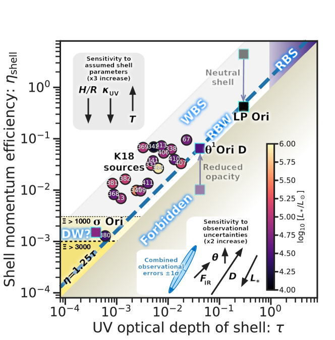
Figure 1: Observational diagnostic diagram for bow shocks. The shell optical depth $\tau$ ($x$ axis) and momentum efficiency $\eta_{\text{sh}}$ ($y$ axis) can be estimated from observations of the bolometric stellar luminosity, infrared shell luminosity, and shell radius, as described in the text. Results are shown for the 20 sources (circle symbols) from Kobulnicky et al. (2018) plus three further sources (square symbols), where we have obtained the measurements ourselves (see Tab. 1). The color of each symbol indicates the stellar luminosity (dark to light) as indicated by the scale bar. The shell pressure is determined assuming a gas temperature $T=${10}^{4}\text{\,}\mathrm{K}$$, an absorption opacity $\kappa=$600\text{\,}\mathrm{c}\mathrm{m}^{2}\,\mathrm{g}^{-1}$$, and a thickness-to-radius ratio $H/R=0.25$. The sensitivity of the results to a factor-of-three change in each parameter is shown in the upper inset box. Exceptions are the two Orion Nebula sources, $\theta^{1}$ Ori D and LP Ori, where the small dim squares show the results of assuming the standard shell parameters, while the large squares show the results of modifications according to the peculiar circumstances of each object, as described in the text. The lower inset box shows the sensitivity of the results to a factor-of-two uncertainty in each observed quantity: distance to source $D$; stellar luminosity $L_{*}$, shell infrared flux $F_{\text{IR}}$; shell angular size $\theta$. Lines and shading indicate different theoretical bow regimes (see Paper I and Paper II). The dashed blue diagonal line corresponds to radiation-supported bows, while the upper left region corresponds to wind-supported bows. The upper right corner (purple) corresponds to optically thick bow shocks, while the lower left corner (yellow) is the region where grain–gas separation may occur, leading to a potential dust wave. However, the existence of a dust wave in this region is not automatic, since it only includes one of the four necessary conditions (§§ 4.4 and 5.1 of Paper II). The lower-right region is strictly forbidden, except in case of violation of the assumption that dust heating be dominated by stellar radiation.

A fundamental parameter is the optical depth, $\tau$, of the bow shell to UV radiation, which determines what fraction of the stellar photon momentum is available to support the shell (see § 2.1 of Paper I). But the same photons also heat the dust grains in the bow, which re-radiate that energy predominantly at mid-infrared wavelengths (roughly $10\text{\,}\mathrm{\SIUnitSymbolMicro m}100\text{\,}\mathrm{\SIUnitSymbolMicro m}$) with luminosity $L_{\text{IR}}$. Assuming that Ly$\alpha$ and mechanical heating of the dust shell is negligible (see § 4.1) and that the emitting shell subtends a solid angle $\Omega$, as seen from the star, then the optical depth can be estimated as

$$\tau=-\ln\left(1-\frac{4\pi}{\Omega}\frac{L_{\text{IR}}}{L_{*}}\right)\approx\frac{2L_{\text{IR}}}{L_{*}}\ ,$$ (1)

where the last approximate equality holds if $\tau\ll 1$ and the shell emission covers one hemisphere.

A second important parameter is the thermal plus magnetic pressure in the shocked shell, which is doubly useful since in a steady state it is equal to both the internal supporting pressure (wind ram pressure plus absorbed stellar radiation) and the external confining pressure (ram pressure of ambient stream). The shell pressure is not given directly by the observations, but can be determined by the following three steps:

1. The shell mass column ($\mathrm{g}\,\mathrm{c}\mathrm{m}^{-2}$) can be estimated from the optical depth by assuming an effective UV opacity: $\Sigma_{\text{sh}}=\tau/\kappa$

2. The shell density ($\mathrm{g}\,\mathrm{c}\mathrm{m}^{-3}$) can be found from the mass column if the shell thickness is known: $\rho_{\text{sh}}=\Sigma_{\text{sh}}/h_{\text{sh}}$. In the absence of other information, a fixed fraction of the shell radius can be used. In particular, we normalize by a typical value of one quarter the star–apex distance: $h_{1/4}=h_{\text{sh}}/(0.25R_{0})$. This corresponds to a Mach number $\mathcal{M}_{0}=\surd 3$ if the stream shock is radiative, or $\mathcal{M}_{0}\gg 1$ if non-radiative (see § 3.2 of Paper I). Further discussion is given in § 5.2 below.

3. Finally, the pressure ($\mathrm{d}\mathrm{y}\mathrm{n}\mathrm{e}\,\mathrm{c}\mathrm{m}^{-2}$) follows by assuming values for the sound speed and Alfvén speed: $P_{\text{sh}}=\rho_{\text{sh}}(c_{\text{s}}^{2}+\frac{1}{2}v_{\scriptscriptstyle\text{A}}^{2})$.

It is natural to normalize this pressure to the stellar radiation pressure at the shell, so we define a shell momentum efficiency

$$\eta_{\text{sh}}\equiv\frac{P_{\text{sh}}}{P_{\text{rad}}}=\frac{4\pi R_{0}^{2}\,(c_{\text{s}}^{2}+\frac{1}{2}v_{\scriptscriptstyle\text{A}}^{2})\,c\,\tau}{L_{*}\,\kappa\,h_{\text{sh}}}\approx 245\frac{R_{\text{pc}}\,T_{4}\,\tau}{L_{4}\,\kappa_{600}\,h_{1/4}}\ ,$$ (2)

where $c$ is the speed of light. In the last step we have assumed ionized gas at temperature $${10}^{4}$\,T_{4}\,$\mathrm{K}$$ with negligible magnetic support ($v_{\scriptscriptstyle\text{A}}\ll c_{\text{s}}$) and written the stellar luminosity and shell parameters in terms of typical values, which we summarize below. Note that the shell momentum efficiency is simply the reciprocal of the radiation parameter from Paper II’s equation (23): $\eta_{\text{sh}}=\Xi_{\text{sh}}^{-1}$, which provides yet a third use for $\eta_{\text{sh}}$, since $\Xi$ is paramount in determining whether the grains and gas remain well-coupled (see § 4.4 of Paper II).

In this section and the remainder of the paper, we employ dimensionless versions of the stellar bolometric luminosity, $L_{*}$, wind mass-loss rate, $\dot{M}$, and terminal velocity, $V_{\text{w}}$, together with the ambient stream’s mass density, $\rho$, relative velocity $v_{\infty}$, and effective dust opacity, $\kappa$. These are defined as follows:

$$\dot{M}_{-7} =\dot{M}/\bigl{(}${10}^{-7}\text{\,}\mathrm{M}_{\odot}\,\mathrm{y}\mathrm{r}^{-1}$\bigr{)}$$

$$V_{3} =V_{\text{w}}/\bigl{(}$1000\text{\,}\mathrm{k}\mathrm{m}\,\mathrm{s}^{-1}$\bigr{)}$$

$$L_{4} =L_{*}/\bigl{(}${10}^{4}\text{\,}\mathrm{L}_{\odot}$\bigr{)}$$

$$v_{10} =v_{\infty}/\bigl{(}$10\text{\,}\mathrm{k}\mathrm{m}\,\mathrm{s}^{-1}$\bigr{)}$$

$$n =(\rho/\bar{m})/\bigl{(}$1\text{\,}\mathrm{c}\mathrm{m}^{-3}$\bigr{)}$$

$$\kappa_{600} =\kappa/\bigl{(}$600\text{\,}\mathrm{c}\mathrm{m}^{2}\,\mathrm{g}^{-1}$\bigr{)}\ ,$$

where $\bar{m}$ is the mean mass per hydrogen nucleon ($\bar{m}\approx 1.3m_{\text{p}}\approx$2.17\text{\times}{10}^{-24}\text{\,}\mathrm{g}$$ for solar abundances).

3 The $\eta_{\text{sh}}$–$\tau$ diagnostic diagram

Table 1: Key observational parameters for star/bow systems

Star	$L_{*}/${10}^{4}\text{\,}\mathrm{L}_{\odot}$$	$L_{\text{IR}}/$\mathrm{L}_{\odot}$$	$R_{0}/$\mathrm{p}\mathrm{c}$$
$\theta^{1}$ Ori D	$2.95$	$620$	$0.003$
LP Ori	$0.16$	$240$	$0.01$
$\sigma$ Ori	$6.0$	$15$	$0.12$
K18 Sources	$1.487$	$82800$	$0.021.35$

In Figure 1 we show the resultant diagnostic diagram: $\eta_{\text{sh}}$ versus $\tau$. The horizontal axis shows the fraction of the stellar radiative energy that is reprocessed by the bow shell, while the vertical axis shows the fraction of stellar radiative momentum that is imparted to the shell, either directly by absorption, or indirectly by the stellar wind (which is itself radiatively driven). Radiatively supported bows (DW, RBW, or RBS cases) should lie on the diagonal line $\eta_{\text{sh}}=(Q_{P}/Q_{\text{abs}})\tau\approx 1.25\tau$, where we have used the ratio of grain radiation pressure efficiency to absorption efficiency found in the FUV band for the dust mixture shown in Paper II’s Figure 6. Wind-supported bows should lie above this line and no bows should lie below the $\eta_{\text{sh}}=\tau$ line, since $Q_{P}$ cannot be smaller than $Q_{\text{abs}}$.

We have calculated $\eta_{\text{sh}}$ and $\tau$ using the above-described methods for the 20 mid-infrared sources studied by Kobulnicky et al. (2018) (K18) and plotted them on our diagnostic diagram. Details of our treatment of this observational material are provided in the following subsection. In order to expand the range of physical conditions, we have included three additional sources (data in Table 1): bows around $\theta^{1}$ Ori D (Smith et al., 2005) and LP Ori (O’Dell, 2001) in the Orion Nebula, which show larger optical depths, plus the inner bow around $\sigma$ Ori, which illuminates the Horsehead Nebula and has previously been claimed to be a dust wave (Ochsendorf et al., 2014; Ochsendorf & Tielens, 2015). Details of the observations of these additional sources will be published elsewhere.

3.1 Treatment of sources from Kobulnicky et al.

In a series of papers Kobulnicky et al. provide an extensive mid-infrared-selected sample of over 700 candidate stellar bow shock nebulae (Kobulnicky et al., 2016, 2017; Kobulnicky et al., 2018, hereafter K16, K17, and K18). For 20 of these sources, reliable distances and spectral classifications are provided in Table 5 of K17 and Tables 1 and 2 of K18. In this section, we outline how we obtain $\tau$ and $\eta_{\text{sh}}$ from the data in these catalogs, while further aspects of the Kobulnicky et al. material are discussed in § 5.2. As this paper was being written, we became aware of a new mass-loss study that greatly expands on the earlier results of K18 (H. Kobulnicky, priv. comm.). The new study includes 70 bow shock sources and incorporates Gaia distances and proper motions, together with new optical/IR spectroscopy of the central stars. Apart from making use of an updated spectral classification of one source (§ 6.4), we have elected to concentrate on only the published K18 sample in this paper, but will address the expanded sample in future publications.

The UV optical depth of the bow shell is obtained (eq. [1]) from the ratio of infrared shell luminosity to stellar luminosity. The inverse of this ratio is given in Table 5 of K17, but we choose to re-derive the values since the spectral classification of some of the sources was revised between K17 and K18. Although K17 found the total shell fluxes from fitting dust emission models to the observed SEDs, we adopt the simpler approach of taking a weighted sum of the flux densities $F_{\nu}$ (in $\mathrm{J}\mathrm{y}$) in three mid-infrared bands:

$$F_{\text{IR}}\approx\bigl{[}2.4\,(F_{8}\text{ or }F_{12})+1.6\,(F_{22}\text{ or }F_{24})\\ +0.51\,F_{70}\bigr{]}\,\times${10}^{-10}\text{\,}\mathrm{e}\mathrm{r}\mathrm{g}\,\mathrm{s}^{-1}\,\mathrm{c}\mathrm{m}^{-2}$\ ,$$ (3)

where $F_{8}$ is Spitzer IRAC $8.0\text{\,}\mathrm{\SIUnitSymbolMicro m}$, $F_{24}$ is Spitzer MIPS $23.7\text{\,}\mathrm{\SIUnitSymbolMicro m}$, $F_{12}$ and $F_{22}$ are WISE bands 3 and 4, and $F_{70}$ is Herschel PACS $70\text{\,}\mathrm{\SIUnitSymbolMicro m}$. The weights are chosen so that the integral $\int_{0}^{\infty}F_{\nu}\,d\nu$ is approximated by the quadrature sum $\Sigma_{k}F_{k}\,\Delta\nu_{k}$, under the assumption that fluxes in shorter (e.g., IRAC $5.8\text{\,}\mathrm{\SIUnitSymbolMicro m}$) and longer (e.g., PACS $150\text{\,}\mathrm{\SIUnitSymbolMicro m}$) wavebands are negligible. Shell fluxes are converted to luminosities using the assumed distance to each source, and stellar luminosities are taken directly from K18 Table 2, based on spectroscopic classification and the calibrations of gravity and effective temperature from Martins et al. (2005).

Figure 2: Comparison between shell-to-star luminosity ratios calculated as described in the text ($y$ axis) with those given in K17 ($x$ axis). The blue dashed line signifies equality and the gray band shows ratios between 1/2 and 2.

In Figure 2 we compare the $\tau$ obtained using the shell luminosity as described above with that obtained using the luminosity ratios directly from K17 Table 5. It can be seen that for the majority of sources the two measurements are consistent within a factor of two (gray band). The four furthest-flung outliers can be understood as follows:

Source 67

This has a very poor-quality spectral fit in K17 (see lower left panel of their Fig. 12) and so $F_{\text{IR}}$ is overestimated by them by a factor of 10.

Sources 341 and 342

The spectral classes changed from B2V in K17 to O9V and B1V, respectively, in K18, increasing the derived $L_{*}$, which lowers $\tau$.

Source 411

The luminosity class changed from Ib (K17) to V (K18), so $L_{*}$ has been greatly reduced, which increases $\tau$.

3.2 Random uncertainties due to observational errors

The fundamental observational quantities that go into determining $\tau$ and $\eta_{\text{sh}}$ for each source are distance, $D$; stellar luminosity, $L_{*}$; total infrared flux, $F_{\text{IR}}$; and bow angular apex distance, $\theta$. From these, the shell radius and infrared luminosity are found as $R_{0}=\theta D$ and $L_{\text{IR}}=4\pi D^{2}F_{\text{IR}}$. Rather than clutter the diagram with error bars, we instead show the sensitivity to observational errors in the lower-right box, where each arrow corresponds to a factor of two increase (0.3 dex) in each quantity: $D$, $L_{*}$, $F_{\text{IR}}$, and $\theta$. We now calculate uncertainty estimates for individual observational quantities that are used in deriving not only $\tau$ and $\eta_{\text{sh}}$ but also mass-loss rates, as discussed later in § 5.

3.2.1 Distance

Most sources are members of known high-mass clusters with distance uncertainties less than 20% (0.08 dex). The only exception is Source 329 in Cygnus, for which the distance uncertainty is roughly a factor of 2 (Kobulnicky et al., 2018).

3.2.2 Stellar luminosity

The stellar luminosity is determined from spectral classification, which makes it independent of distance. Taking a $2000\text{\,}\mathrm{K}$ dispersion in the effective temperature scale (Martins et al., 2005) gives an uncertainty of 25% in the luminosity, and adding in possible errors in gravity and the effect of binaries, we estimate a total uncertainty in $L_{*}$ of 50% (0.45 mag or 0.18 dex).

3.2.3 Shell flux and surface brightness

We estimate the uncertainty in shell bolometric flux, $F_{\text{IR}}$, by comparing two different methods: model fitting (Kobulnicky et al., 2017) and a weighted sum of the 8, 24, and $70\text{\,}\mathrm{\SIUnitSymbolMicro m}$ bands (eq. [3]), giving a standard deviation of 17% (0.07 dex). To this, we add the estimate of 25% for the effects of background subtraction uncertainties on individual photometric measurements (Kobulnicky et al., 2017). The absolute flux calibration uncertainty for both Herschel PACS (Balog et al., 2014) and Spitzer MIPS (Engelbracht et al., 2007) is less than 5%, which is small in comparison. Combining the 3 contributions in quadrature gives a total uncertainty of 0.12 dex. We adopt the same uncertainty for the $70\text{\,}\mathrm{\SIUnitSymbolMicro m}$ surface brightness.

3.2.4 Angular sizes

For the angular apex distance, $\theta$, the largest uncertainty for well-resolved sources is due to the unknown inclination. Tarango-Yong & Henney (2018) show that the dispersion in true to projected distances can introduce an uncertainty of $30\%$ (0.11 dex) in unfavorable cases (e.g., their Fig. 26). For 5 of the 20 sources from Kobulnicky et al. (2018), $\theta$ is of order the Spitzer PSF width at $24\text{\,}\mathrm{\SIUnitSymbolMicro m}$, so the errors may be larger.

3.2.5 Stellar wind velocity

Although this is not strictly an observed quantity for the K18 sample, we will treat it as such since it is estimated per star, based on the spectral type. K18 estimate 50% uncertainty, and we adopt the same here (0.18 dex).

3.2.6 Combined effect of uncertainties on the $\tau$–$\eta_{\text{sh}}$ diagram

Assuming that the uncertainty in each observational quantity is independent, we can now combine them using the techniques described in Appendix A to find the $\pm 1~{}\sigma$ error ellipse, shown in blue in the figure. It can be seen that observational uncertainties in $\tau$ and $\eta_{\text{sh}}$ are highly correlated: the dispersion is $0.7\text{\,}\mathrm{d}\mathrm{e}\mathrm{x}$ in the product $\eta_{\text{sh}}\tau$ but only $0.16\text{\,}\mathrm{d}\mathrm{e}\mathrm{x}$ in the ratio $\eta_{\text{sh}}/\tau$, with stellar luminosity errors dominating in both cases. Observational uncertainties are therefore relatively unimportant in determining whether a given source is wind-driven or radiation-driven, which depends only on $\eta_{\text{sh}}/\tau$. On the other hand, they do significantly affect the question of whether a source has a sufficiently high radiation parameter $\Xi$ to possibly be a dust wave.

3.3 Systematic uncertainties due to assumed shell parameters

A further source of uncertainty arises from the parameters of the shocked shell that are assumed in steps P1–P3. Namely, the relative shell thickness, $h_{\text{sh}}/R_{0}$, the ultraviolet grain opacity per mass of gas, $\kappa$, and the shell temperature, $T$. These parameters effect only $\eta_{\text{sh}}$, not $\tau$, with a sensitivity shown by arrows in the upper left box of Figure 1.

3.3.1 Shell thickness

For maximally efficient post-shock radiative cooling, the shell thickness depends on the Mach number of the shock as $h/R_{0}\sim M_{0}^{-2}$. However, for ambient densities less than about $10\text{\,}\mathrm{c}\mathrm{m}^{-3}$, the minimum thickness is only about ten times smaller than the $h/R_{0}=0.25$ that we are assuming. In photoionized gas, this occurs at $v\approx$60\text{\,}\mathrm{k}\mathrm{m}\,\mathrm{s}^{-1}$$, corresponding to the peak in the cooling curve at ${10}^{5}\text{\,}\mathrm{K}$ (see § 3.2 of Paper I), since the thickness is set by the cooling length at higher speeds. In the case that the Alfvén speed is a significant fraction of the sound speed, this will also tend to increase the thickness. In principle, the shell thickness can be measured observationally if the source is sufficiently well resolved (Kobulnicky et al., 2017), although this is complicated by projection effects. We return to the issue of the shell thickness in the discussion below.

3.3.2 Dust opacity

The dust opacity will depend on the total dust-gas ratio and on the composition and size distribution of the grains. Our adopted value of $600\text{\,}\mathrm{c}\mathrm{m}^{2}\,\mathrm{g}^{-1}$, or $1.3\text{\times}{10}^{-21}\text{\,}\mathrm{c}\mathrm{m}^{2}\,\mathrm{H}^{-1}$, is appropriate for average Galactic interstellar grains in the EUV and FUV (e.g., Weingartner & Draine, 2001), but there is ample evidence for substantial spatial variations in grain extinction properties (Fitzpatrick & Massa, 2007), both on Galactic scales (Schlafly et al., 2016) and within a single star forming region (Beitia-Antero & Gómez de Castro, 2017). The properties of grains within photoionized regions are very poorly constrained observationally because the optical depth is generally much lower than in overlying neutral material. In the Orion Nebula, there is some evidence (Salgado et al., 2016) that the FUV dust opacity in the ionized gas may be as low as $90\text{\,}\mathrm{c}\mathrm{m}^{2}\,\mathrm{g}^{-1}$, although the uncertainties in this estimate are large and different results are obtained in other regions, such as W3(A) (Salgado et al., 2012). It is even possible that the FUV dust opacity may be larger than the ISM value if the abundance of very small grains is enhanced through radiative torque disruption of larger grains (Hoang et al., 2018).

3.3.3 Shell gas temperature

For bows around O stars, the shell temperature should be close to the photoionization equilibrium value of $\approx${10}^{4}\text{\,}\mathrm{K}$$, since the post-shock cooling length is short in ambient densities above $0.1\text{\,}\mathrm{c}\mathrm{m}^{-3}$ and the shell does not trap the ionization front for ambient densities below ${10}^{4}\text{\,}\mathrm{c}\mathrm{m}^{-3}$ (see Paper I’s §§ 3.1 and 3.2 for details). For B stars, on the other hand, these two density limits move closer together, making it more likely that a bow will lie in a different temperature regime. The only source for which we have evidence that this occurs is LP Ori, as discussed in the next section.

3.4 Special treatment of particular sources

For two of the additional bows listed in Table 1, we are forced to deviate from the default values for the shell parameters. For LP Ori, the bow shell appears to be formed from neutral gas (O’Dell, 2001) and its relatively high $\tau$ value is more than sufficient to trap the weak ionizing photon output of a B3 star. We therefore move its point in Figure 1 downward by a factor of ten, which could be a thermally supported neutral shell at $2000\text{\,}\mathrm{K}$ or a magnetically supported shell with $v_{\scriptscriptstyle\text{A}}\approx$3\text{\,}\mathrm{k}\mathrm{m}\,\mathrm{s}^{-1}$$). For the case of the Orion Trapezium star $\theta^{1}$ Ori D, we find that using the default parameters results in a placement well inside the forbidden zone of Figure 1 (indicated by fainter symbol). For this object there is no reason to suspect anything but the usual photoionized temperature of ${10}^{4}\text{\,}\mathrm{K}$, but its placement could be resolved either by decreasing the shell thickness, or decreasing the UV dust opacity, or both. Given the moderate limb brightening seen in the highest resolution images of the Ney–Allen nebula (Robberto et al., 2005; Smith et al., 2005), the shell thickness is unlikely to be less than half our default value. But, if this were combined with a factor 5 decrease in $\kappa$, as suggested by Salgado et al. (2016), then this would be sufficient to move the source up to the RBW line, or slightly above.

3.5 Candidate radiation-supported bows

Four sources are sufficiently close to the diagonal line $\eta_{\text{sh}}=1.25\tau$ in Figure 1 that they should be treated as strong candidates for radiation-supported bows. These are K18 sources 380 (HD 53367, V750 Mon) and 407 (HD 93249 in Carina) plus $\theta^{1}$ Ori D and LP Ori. Of the four, source 380 is the only one that is also a candidate for grain-gas decoupling. Further details of the two K18 sources are presented in Appendix B, where for source 380 we show that reducing both luminosity and distance by a factor of roughly 2 with respect to the values used by K18 would provide a better fit to the totality of observational data. However, the ratio $\eta_{\text{sh}}/\tau$ is proportional to $D/L_{*}$ so it would not be affected by such an adjustment and the bow remains radiation-supported. On the other hand $\eta_{\text{sh}}$ (proportional to $D/L_{*}^{2}$) would increase by 2, making the classification as dust wave candidate more marginal.

Three additional K18 sources (409, 410, 411) are within a factor of 3 of the radiation-supported line, so they too must be considered as potential candidates, given our estimated systematic uncertainty in the shell parameters (§ 3.3).

4 Mid-infrared grain emissivity

In preparation for our discussion of different wind mass-loss diagnostic methods below, in this section we calculate the grain emissivity predicted by models of dust heated by a nearby OB star. We use the same simulations that we employed in § 4.2 of Paper II, which employ the plasma physics code Cloudy (Ferland et al., 2013, 2017). In summary, simulations of spherically symmetric, steady-state, constant density H ii regions were carried out for four different stellar types from B1.5 to O5 (Table 2 of Paper II), a range of gas densities from $1\text{\,}\mathrm{c}\mathrm{m}^{-3}{10}^{4}\text{\,}\mathrm{c}\mathrm{m}^{-3}$, and using Cloudy’s default “ISM” graphite/silicate dust mixture with 10 size bins from $0.005\text{\,}\mathrm{\SIUnitSymbolMicro m}0.25\text{\,}\mathrm{\SIUnitSymbolMicro m}$.

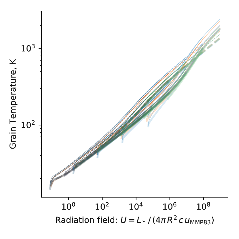
Figure 3: Grain temperature versus radiation field mean intensity, $U$, in units of the interstellar radiation field in the solar neighborhood. Line types and colors correspond to a variety of stellar spectral shapes, gas densities, and grain species. Dashed lines show carbon grains, solid lines show silicate grains, with line thickness and transparency increasing with grain size. Stellar spectral types are O5 V (blue), O9 V (orange), B1.5 V (purple), and B0.7 Ia (green), with lighter shades denoting higher gas densities.

Figure 3 shows equilibrium grain temperatures for these Cloudy models as a function of the nominal energy density of the radiation field, $U=u/u_{\text{\tiny MMP83}}$, where $u=L/4\pi R^{2}c$ and $u_{\text{\tiny MMP83}}$ is the energy density of the interstellar radiation field for $\lambda<$8\text{\,}\mathrm{\SIUnitSymbolMicro m}$$ in the solar neighborhood (Mathis et al., 1983):

$$u_{\text{\tiny MMP83}}\,c=$0.0217\text{\,}\mathrm{e}\mathrm{r}\mathrm{g}\,\mathrm{s}^{-1}\,\mathrm{c}\mathrm{m}^{-2}$\ .$$ (4)

The tight relationship seen in Figure 3 between $T$ and $U$ is evidence for the dominance of stellar radiative heating, which we justify on theoretical grounds in § 4.1 below. The variation about the mean relation is mainly due to differences in grain size and composition, with smaller grains and graphite grains being relatively hotter. The downward hooks seen on the left end of each simulation’s individual curve are due to the fact that our calculation of $U$ does not account for internal absorption, which starts to become important near the ionization front.

Figure 4: Grain emissivity at $70\text{\,}\mathrm{\SIUnitSymbolMicro m}$ for all Cloudy models, with lines colored as in Fig. 3, but without the variation in line type and thickness since emissivity is integrated over all grain types and sizes. For comparison, the emissivity from the grain models of Draine & Li (2007) are shown as dark gray symbols, which assume illumination by a scaled interstellar radiation field with a SED with a very different shape from that of an OB star, see Fig. 5. The light gray symbols show the effect of using an 8 times higher $U$ with the Draine & Li models, which approximately compensates for this difference in SED.

The grain emissivity at $70\text{\,}\mathrm{\SIUnitSymbolMicro m}$ (Herschel PACS blue band) for the Cloudy simulations (colored lines) is shown in Figure 4, where it is compared with the same quantity from the grain models (dark gray symbols) of Draine & Li (2007). A clear difference is seen between the two sets of models, but this is due almost entirely to a difference in the assumed spectrum of the illuminating radiation, as illustrated in Figure 5. Draine & Li (2007) use a SED that is typical of the interstellar radiation field in the Galaxy, which is dominated by an old stellar population, which peaks in the near infrared, with only a small FUV contribution from younger stars (about 8% of the total energy density). This is very different from the OB star SEDs, which are dominated by the FUV and EUV bands. Since the grain absorption opacity is substantially higher at UV wavelengths than in the visible/IR (see Fig. 6 of Paper II), the effective grain heating efficiency of the OB star SED is correspondingly higher. The light gray symbols show the effect on the Draine & Li (2007) models of multiplying the radiation field by a factor of $8$ in order to offset this difference in efficiency, which can be seen to bring them into close agreement with the Cloudy models. A further difference is that the Draine & Li (2007) model includes small PAH particles, which we do not include in our Cloudy models, since they are believed to be largely absent in photoionized regions (Giard et al., 1994; Lebouteiller et al., 2011). However, this only effects the emissivity at shorter mid-infrared wavelengths $<$20\text{\,}\mathrm{\SIUnitSymbolMicro m}$$.

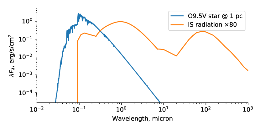
Figure 5: Comparison between the spectral energy distribution (SED) of a typical OB star (blue line) and the interstellar radiation field in the solar neighborhood (orange line). The OB star is the $20\text{\,}\mathrm{M}_{\odot}$ model from Table 1 of Paper I and is plotted for a distance from the star of $1\text{\,}\mathrm{p}\mathrm{c}$. The interstellar SED is from Mathis et al. (1983) and is multiplied by $80$ so that the total FUV-to-NIR flux is equal for the two SEDs.

In terms of the characteristic parameters introduced in § 2 the dimensionless radiation field becomes

$$U=14.7\,L_{4}\,R_{\text{pc}}^{-2}\ ,$$ (5)

or, alternatively, it can be expressed in terms of the ambient stream as

$$U=3.01\,n_{\infty}\,v_{10}^{2}/x^{2}\ ,$$ (6)

where $x=R_{0}/R_{*}$ is given by Paper I’s equation (12). It can also be related to the radiation parameter $\Xi$, defined in Paper II’s equation (23), as

$$U=3.82\,nT_{4}\,\Xi\ .$$ (7)

A common alternative approach to scaling the radiation field (see Tielens & Hollenbach, 1985 and citations thereof) is to normalize in the FUV band ($0.0912\text{\,}\mathrm{\SIUnitSymbolMicro m}0.24\text{\,}\mathrm{\SIUnitSymbolMicro m}$), where the local interstellar value is known as the Habing flux (Habing, 1968):

$$F_{\text{\tiny Habing}}=$0.0016\text{\,}\mathrm{e}\mathrm{r}\mathrm{g}\,\mathrm{s}^{-1}\,\mathrm{c}\mathrm{m}^{-2}$\ .$$ (8)

The resultant dimensionless flux is often denoted by $G_{0}$, and the relationship between $G_{0}$ and $U$ depends on the fraction $f_{\text{fuv}}$ of the stellar luminosity that is emitted in the FUV band:

$$G_{0}=f_{\text{fuv}}\frac{u_{\text{\tiny MMP83}}\,c}{F_{\text{\tiny Habing}}}\,U=(\text{$610$})\,U\ ,$$ (9)

where we give the range corresponding to early O ($f_{\text{fuv}}\approx 0.4$) to early B ($f_{\text{fuv}}\approx 0.7$) stars.

4.1 Unimportance of other heating mechanisms

The grain temperature in bows around OB stars is determined principally by the steady-state equilibrium between the absorption of stellar UV radiation (heating) and the thermal emission of infrared radiation (cooling). Other processes such as single-photon stochastic heating, Lyman $\alpha$ line radiation, and post-shock collisional heating can dominate in other contexts, but these are generally unimportant for circumstellar bows, as we now demonstrate.

4.1.1 Stochastic single-photon heating

When the radiation field is sufficiently dilute, then a grain that absorbs a photon has sufficient time to radiate all that energy away before it absorbs another photon (Duley, 1973). In this case, the emitted infrared spectrum for $\lambda<$50\text{\,}\mathrm{\SIUnitSymbolMicro m}$$ becomes relatively insensitive of the energy density of the incident radiation (Draine & Li, 2001). However, this is most important for the very smallest grains. From equation (47) of Draine & Li (2001), one finds that grains with sizes larger than $a=$0.005\text{\,}\mathrm{\SIUnitSymbolMicro m}$=$5\text{\,}\mathrm{n}\mathrm{m}$$ (the smallest size included in our Cloudy models) should be close to thermal equilibrium for $U>30$, which is small compared with typical bow shock values ($U=\text{${10}^{3}{10}^{6}$}$). As mentioned above, PAHs are not expected to be present in the interior of H ii regions. Desert et al., 1990 found them to be strongly depleted for $U>100$ around O stars. However, other types of ultra-small grains, down to sub-nm sizes (Xie et al., 2018) may be present in bows, and stochastic heating would be important for grains with $a=$1\text{\,}\mathrm{n}\mathrm{m}$$ if $U<${10}^{5}$$. Note, however that grains smaller than $0.6\text{\,}\mathrm{n}\mathrm{m}$ would be destroyed by sublimation after absorbing a single He-ionizing photon.

4.1.2 Lyman $\alpha$ heating

On the scale of an entire H ii region, the dust heating is typically dominated by Lyman $\alpha$ hydrogen recombination line photons, which are trapped by resonant scattering (e.g., Spitzer, 1978 § 9.1b). However, this is no longer true on the much smaller scale of typical bow shocks. An upper limit on the Lyman $\alpha$ energy density can be found by assuming all line photons are ultimately destroyed by dust absorption rather than escaping in the line wings (e.g., Henney & Arthur, 1998), which yields

$$U_{\text{Ly}\alpha}\approx 0.1n/\kappa_{600}\ .$$ (10)

This can be combined with equation (6) to give the ratio of Lyman $\alpha$ to direct stellar radiation as

$$\frac{U_{\text{Ly}\alpha}}{U}\approx 0.03\frac{x^{2}}{v_{10}^{2}\kappa_{600}}\ .$$ (11)

Taking the most favorable parameters imaginable of a slow stream ($v_{10}=2$), very strong wind ($x\approx 1$), and reduced dust opacity ($\kappa_{600}=0.1$) gives a Lyman $\alpha$ contribution of only 10% of the stellar radiative energy density. In any other circumstances, the fraction would be even lower.

4.1.3 Shock heating

The outer shock thermalizes the kinetic energy of the ambient stream, which may in principle contribute to the infrared emission of the bow. In order for this process to be competitive, the following three conditions must all hold:

1. The post-shock gas must radiate efficiently with a cooling length less than the bow size, see § 3.2 of Paper I. This is satisfied for all but the lowest densities (Paper I’s Fig. 2).

2. A significant fraction of the shock energy must be radiated by dust. This requires that the post-shock temperature be greater than ${10}^{6}\text{\,}\mathrm{K}$, which requires a stream velocity $v_{\infty}>$200\text{\,}\mathrm{k}\mathrm{m}\,\mathrm{s}^{-1}$$ (Draine, 1981). This also coincides with the range of shock velocities where the smaller grains will start to be destroyed by sputtering in the post-shock gas.

3. The kinetic energy flux through the shock must be significant, compared with the fraction of the stellar radiation flux that is absorbed and reprocessed by the bow shell.

It turns out that the third condition is the most stringent, so we will consider it in detail. The kinetic energy flux through the outer shock for an ambient stream of density $\rho_{\infty}$ and velocity $v_{\infty}$ is

$$F_{\text{kin}}=\tfrac{1}{2}\rho_{\infty}v_{\infty}^{3}=\tfrac{1}{2}P_{\text{sh}}v_{\infty}\ ,$$ (12)

while the stellar radiative energy flux absorbed by the shell is

$$F_{\text{abs}}\approx\tau L/4\pi R_{0}^{2}\ ,$$ (13)

assuming an absorption optical depth $\tau\ll 1$. The shell pressure in the WBS case can be equated to the ram pressure of the internal stellar wind (see § 2.1 of Paper I), so that the ratio of the two energy fluxes is

$$\frac{F_{\text{kin}}}{F_{\text{abs}}}=\frac{1}{2}\frac{\eta_{\text{w}}}{\tau}\frac{v_{\infty}}{c}\ .$$ (14)

An upper limit to the stellar wind momentum efficiency $\eta_{\text{w}}$ is the shell momentum efficiency $\eta_{\text{sh}}$ that is derived observationally in § 2, where it is found that $\eta_{\text{sh}}/\tau<30$ for all sources considered. Therefore, for a stream velocity $v_{\infty}=$200\text{\,}\mathrm{k}\mathrm{m}\,\mathrm{s}^{-1}$$, we have $F_{\text{kin}}/F_{\text{abs}}<0.01$ and the shock-excited dust emission is still negligible. Only in stars with $v_{\infty}>$1000\text{\,}\mathrm{k}\mathrm{m}\,\mathrm{s}^{-1}$$ would the shock emission start to be significant, and such hyper-velocity stars (Brown, 2015) do not show detectable bow shocks.

So far, we have only considered the outer shock, but the inner shock that decelerates the stellar wind will have a velocity of $1000\text{\,}\mathrm{k}\mathrm{m}\,\mathrm{s}^{-1}3000\text{\,}\mathrm{k}\mathrm{m}\,\mathrm{s}^{-1}$ and therefore might have a significant kinetic energy flux by eq. (14). However, the stellar wind from hot stars will be free of dust, so that it would be necessary for the stellar wind protons to cross the contact/tangential discontinuity and deposit their energy in the dusty plasma of the shocked ambient stream in order for this source of energy to contribute to the grain emission. This is not possible because the Larmor radius (see § 5 of Paper II) of a $3000\text{\,}\mathrm{k}\mathrm{m}\,\mathrm{s}^{-1}$ proton in a $1\text{\,}\mathrm{\SIUnitSymbolMicro}\mathrm{G}$ field is only $3\text{\times}{10}^{10}\text{\,}\mathrm{c}\mathrm{m}$, which is millions of times smaller than typical bow sizes. The magnetic field in the outer shell is unlikely to be smaller than $\approx n^{1/2}$\mathrm{\SIUnitSymbolMicro}\mathrm{G}$$, given that Alfvén speeds of $2\text{\,}\mathrm{k}\mathrm{m}\,\mathrm{s}^{-1}$ are typical of photoionized regions (Arthur et al., 2011; Planck Collaboration et al., 2016) and if the density were much lower than $1\text{\,}\mathrm{c}\mathrm{m}^{-3}$, then the scale of the bow would be commensurately larger anyway. Three-dimensional MHD simulations of bow shocks (Katushkina et al., 2017; Gvaramadze et al., 2018) show that the magnetic field lines are always oriented parallel to the shell, so that high energy particles from the stellar wind would be efficiently reflected in a very thin layer and cannot contribute to grain heating. For the same reason, heat conduction by electrons across the contact discontinuity is also greatly suppressed (Meyer et al., 2017).

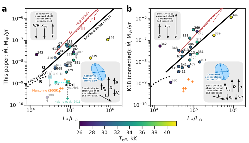
Figure 6: Wind mass-loss rates as a function of stellar luminosity, derived from (a) our trapped energy/momentum method and (b) the grain emissivity method of Kobulnicky et al. (2018), with corrections as described in our § 5.2. Circle symbols show the sources from K18, colored according to the stellar effective temperature (see key at far right). In panel a, squares show two of our additional sources (Tab. 1). Upper limits to the mass loss are given for sources that lie close to the radiation-supported line in Fig. 1, represented by faint symbols and downward-pointing arrows. Sources that lie less than a factor of three above the line have enhanced downward uncertainties and are also shown by slightly fainter symbols. For $\sigma$ Ori, the large symbol corresponds to the sum of the luminosities of the triple OB system Aa, Ab, and B (Simón-Díaz et al., 2015), while the small symbol corresponds to the luminosity of only the most massive component Aa. Lines show the predictions of stellar wind models: red lines are the commonly used recipes from Vink et al. (2000) for dwarfs (solid), giants (dashed), and supergiants (dotted), while black lines show eq. (11) of Krtička & Kubát (2017) for O stars (solid) and models of Krtička (2014) for B stars. Orange plus symbols show mass-loss measurements from NUV lines for weak-wind O dwarfs (Marcolino et al., 2009), while the green plus symbol shows the measurement from infrared H recombination lines for $\sigma$ Ori (Najarro et al., 2011). Boxes show the sensitivity of the results to observational uncertainties (lower right) and assumed shell parameters (upper left).

5 Stellar wind mass-loss rates

Various methods have been proposed to derive stellar wind mass-loss rates from observations of stellar bow shocks for example, Kobulnicky et al., 2010; Gvaramadze et al., 2012; Kobulnicky et al., 2018. In this section, we will show how the $\tau$–$\eta_{\text{sh}}$ diagram can be used to derive the mass-loss rate for bows in the wind-supported regime. We then compare our method with the method used by Kobulnicky et al. (2018), which is a refinement of that originally proposed in Kobulnicky et al. (2010). The method used by Gvaramadze et al. (2012) uses combined measurements of the bow shock and the surrounding H ii region. It has the advantage of depending on fewer free parameters than the other methods, but can only be used in the case of isolated stars, whereas the majority of the sources considered here are in cluster environments.

5.1 Mass loss determination from the $\tau$–$\eta_{\text{sh}}$ diagram

Taking into account the support from stellar wind ram pressure and the absorbed stellar radiation pressure, the pressure of the bow shell can be written

$$\eta_{\text{sh}}=\eta_{\text{w}}+\left(1-e^{-Q_{\text{p}}\tau/Q_{\text{abs}}}\right)\ ,$$ (15)

which is valid in all 3 regimes: WBS, RBW, and RBS. The wind momentum efficiency is defined in terms of the stellar wind parameters (eq. [13] of Paper I):

$$\eta_{\text{w}}=$0.495$\,\dot{M}_{-7}\,V_{3}\,L_{4}^{-1}\ .$$ (16)

Therefore, assuming $Q_{\text{p}}/Q_{\text{abs}}=1.25$ as in § 2, the mass-loss rate can be estimated as

$$\dot{M}_{-7}=2.02\,L_{4}\,V_{3}^{-1}\,\left[\eta_{\text{sh}}-\left(1-e^{-1.25\tau}\right)\right]\ .$$ (17)

In the wind-supported WBS regime ($\tau\ll\eta_{\text{w}}\approx\eta_{\text{sh}}$), the second term in the brackets is negligible, and we can use equations (1, 2) to write

$$\dot{M}_{-7}\approx 990\frac{R_{\text{pc}}\,T_{4}\,L_{\text{IR},4}}{L_{4}\,V_{3}\,\kappa_{600}\,h_{1/4}}\ .$$ (18)

On the other hand, if $\eta_{\text{sh}}$ does not greatly exceed $\tau$, then the full equation (17) should be used, although the uncertainties in $\eta_{\text{sh}}$ and $\tau$, combined with the partial cancellation of two similar-sized terms, mean that the mass loss will be poorly constrained in such cases.

Resulting mass-loss rates are shown as a function of stellar luminosity in Figure 6a for the K18 and Orion sources. As in Figure 1 we show separately the uncertainties in the measurements due to observational errors (lower right box) and systematic model uncertainties (upper left box). Typical observational uncertainties are combined into an error ellipse using the techniques of Appendix A, which is shown in light blue. Sources that are close to the RBW line in the $\tau$–$\eta_{\text{sh}}$ diagram yield only upper limits to the mass-loss rate and these are shown as faint symbols in the figure.

Our results are compared with the commonly used mass-loss recipes of Vink et al. (2000) (red lines) and more recent whole-atmosphere simulations of wind formation in B stars (Krtička, 2014) and O stars (Krtička & Kubát, 2017). Additionally, we show observational mass loss determinations for weak wind O dwarfs (Marcolino et al., 2009) as orange plus symbols. It can be seen that the majority of the K18 sources fall below the Vink et al. line and are more consistent with the Krtička & Kubát (2017) models.

5.2 Mass loss determination method of Kobulnicky et al. (2018)

K18 derive mass-loss rates for their sources using a method that is different from the one that we employ above. Both methods are based on determining the stellar wind ram pressure that supports the bow shell, but K18 do so via the following steps:

1. The line-of-sight mass column through the shell is calculated by combining the peak surface brightness at $70\text{\,}\mathrm{\SIUnitSymbolMicro m}$, $S_{70}$, with a theoretical emissivity per nucleon, $j_{70}(U)$, from Draine & Li (2007): $\Sigma_{\text{los}}=S_{70}/\bar{m}j_{70}(U)$. This depends on knowledge of the stellar radiation field at the shell: $U\propto L_{*}/R_{0}^{2}$.

2. The shell density is found from the line-of-sight mass column using an observationally determined “chord diameter”, $\ell$, which is assumed to be equal to the depth along the line of sight: $\rho_{\text{sh}}=\Sigma_{\text{los}}/\ell$.

3. The internal ram pressure is equated to the external ram pressure, which is found by assuming a stream velocity of $30\text{\,}\mathrm{k}\mathrm{m}\,\mathrm{s}^{-1}$ and a compression factor of 4 across the outer shock: $P_{\text{stream}}=0.25\rho_{\text{sh}}\times($30\text{\,}\mathrm{k}\mathrm{m}\,\mathrm{s}^{-1}$)^{2}$.

There are clear parallels but also differences between steps K1–K3 and our own steps P1–P3. Our step P1 depends on the total observed infrared flux of the bow combined with an assumption about the grain opacity at ultraviolet wavelengths, while step K1 depends on the peak brightness at a single wavelength combined with an assumption about the grain emissivity at infrared wavelengths. Our step P2 requires an assumption about the relative thickness of the shell, while step K2 is more directly tied to observations. On the other hand, step K3 makes a roughly equivalent assumption about the shock compression factor, and a further assumption about the stream velocity. These assumptions are not necessary for our step P3, but we do need to assume a value for the shell gas temperature.

In principle, both methods are valid and their different assumptions and dependencies on observed quantities and auxiliary parameters provide an important cross check on one another. However, as explained in detail in § 4, the $j_{\nu}(U)$ relation depends on the shape of the illuminating SED, which means that the Draine & Li (2007) models require modification when applied to grains around OB stars. A further discrepancy arises due to an interpolation error in K18, which resulted in values of $j_{70}$ being overestimated by about a factor of 2 for sources with weak radiation fields (H. Kobulnicky, priv. comm.).

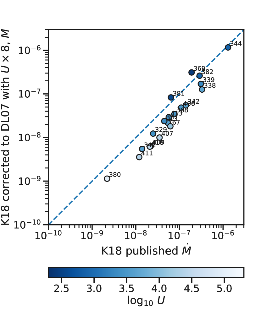
Figure 7: Effects on mass-loss determination of correcting the K18 emissivities. The mass-loss rates from Table 2 of K18 are shown on the $x$ axis, while the corrected values are shown on the $y$ axis. Symbols are color coded by the strength of the radiation field, $U$. The corrected mass-loss rates are predominantly lower by a factor of roughly 2.

After correcting the $70\text{\,}\mathrm{\SIUnitSymbolMicro m}$ emissivities in this way, we re-derive the mass loss rates, following the same steps as in K18, which are then used in Figure 6b above. The difference between these corrected mass-loss rates and those published in K18 is shown in Figure 7. It can be seen that sources with $U\approx${10}^{3}$$ (darker shading) are relatively unaffected but that sources with stronger radiation fields (lighter shading) have their mass-loss increasingly reduced. The average reduction is by a factor of about two.

6 Discussion

In this section we discuss various issues related to our results, beginning in § 6.1 with a consideration of how the optical properties of the grain population in bow shocks might be affected by the extreme radiation environment. This is followed by examination of various sub-groups of sources that are unusual in some way: those where the two mass-loss methods give discrepant results (§ 6.2), those that may be radiation-supported (§ 6.3), and one source that shows a very large apparent mass-loss rate for its luminosity (§ 6.4).

6.1 Evolution of grain size

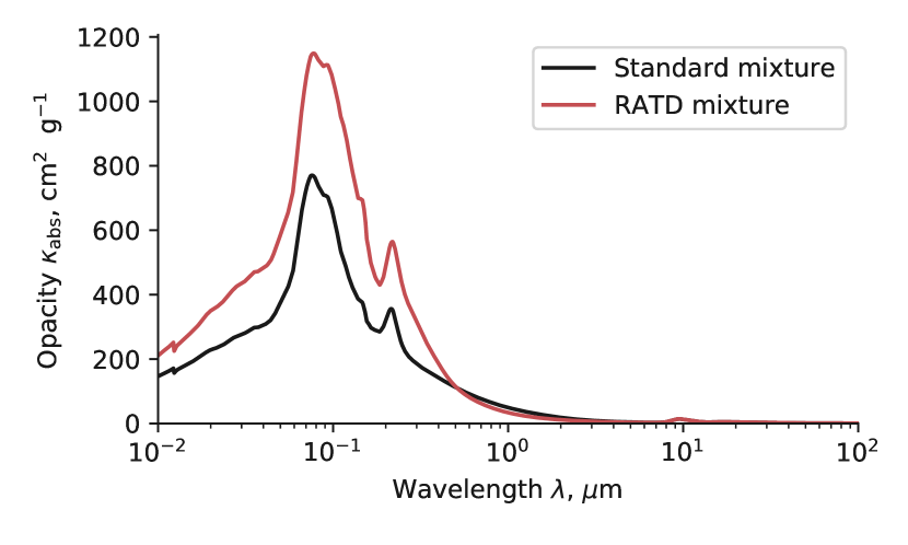
Figure 8: Change in dust opacity due to Radiative Torque Disruption of large grains. Black line shows the total absorption opacity of Cloudy’s standard ISM dust mixture. The red line shows the result of simulating the RATD process by removing the grains larger than $0.04\text{\,}\mathrm{\SIUnitSymbolMicro m}$ and distributing their mass among smaller grain sizes.

The properties of dust grains in bow shocks might be significantly different from those in the general interstellar medium, particularly because of the strong radiation field to which they are exposed, which has effects at both the small and large ends of the grain size distribution. At the small end, sub-nanometer sized particles, such as PAHs can be destroyed by hard EUV photons (Lebouteiller et al., 2007; Lebouteiller et al., 2011). Larger grains, on the other hand, are most vulnerable to Radiative Torque Disruption (RATD; Hoang et al., 2018), see discussion in § 6.4 of Paper II. This is important for our diagnostics because it would tend to reduce the average grain size, while maintaining the same total grain mass, which would have the effect of increasing the ultraviolet opacity, while leaving the mid-infrared opacity unchanged. We do not know the exact size distribution of fragments that would result from the RATD process, but we can estimate its effect by assuming that all grains with $a>$0.05\text{\,}\mathrm{\SIUnitSymbolMicro m}$$ are transformed into grains with $a=\text{$0.025\text{\,}\mathrm{\SIUnitSymbolMicro m}0.05\text{\,}\mathrm{\SIUnitSymbolMicro m}$}$. We implement this crudely in the Cloudy grain model (§ 4) by setting to zero the abundance of graphite and silicate grains in size bins 7, 8, 9, 10, while at the same time distributing their mass equally between size bins 5, and 6, which increases the abundance in those bins by factors of 5.19 and 4.45, respectively. The results are shown in Figure 8, which shows the wavelength-dependent absorption opacity $\kappa$ for both the standard ISM grain mixture and this RATD-modified mixture. As expected, the UV opacity is increased in the RATD mixture, but only by about 50%, whereas the near-infrared opacity is decreased and the visual extinction becomes much steeper, which would correspond to a small total-to-selective extinction ratio of $R_{V}<3$.

This modest increase in opacity from RATD grain processing is well within the systematic uncertainties that we have been assuming and so does not invalidate the results of the previous sections. If the larger grains were instead to break up into many small fragments, the effect would be much larger. If we repeat the above exercise, but assuming the fragment size is $<$0.01\text{\,}\mathrm{\SIUnitSymbolMicro m}$$, then we find an increase by a factor of five in the UV opacity, but we do not feel that this is realistic. Studies of the break-up of fast-spinning small asteroids (Hirabayashi, 2015; Zhang et al., 2018) show that when the tensile strength dominates over self-gravity, then stresses are highest in the center of the body, leading to break up into a small number of similarly sized pieces, as observed in asteroid P/2013 R3 (Jewitt et al., 2014). In the case of dust grains, the tensile strength and angular velocity are both far higher than in the asteroid case, but we expect a similar behavior so that the fragment size should be predominantly within a factor of about two below the critical size given in equation (28) of Hoang et al. (2018), as we assumed in Figure 8.

6.2 Why do results of the two mass-loss methods differ?

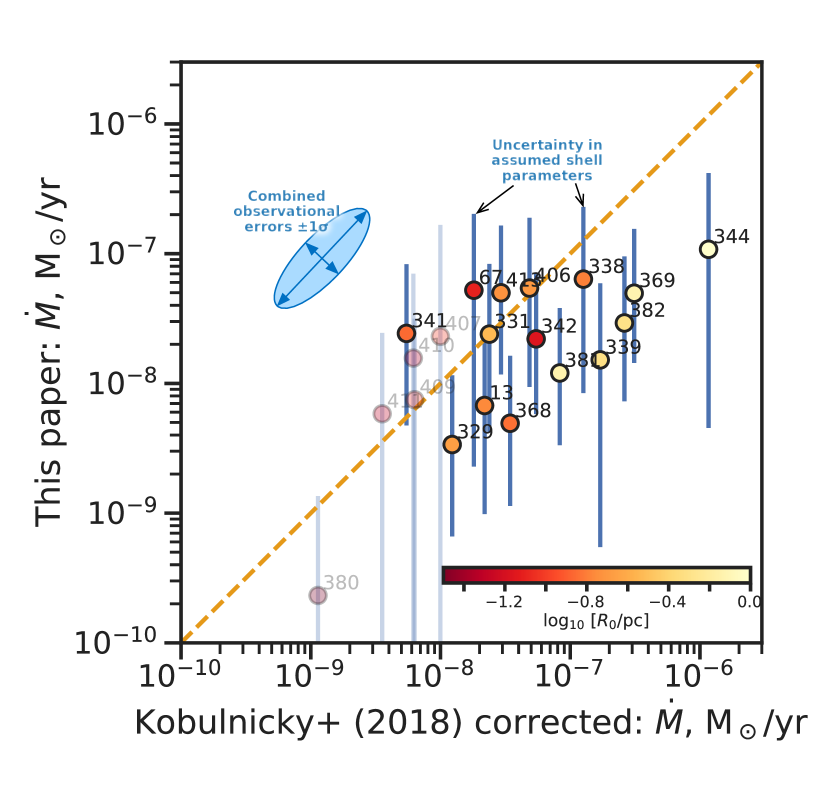
Figure 9: Comparison of the two mass-loss methods: K18 corrected method ($x$ axis) versus our method ($y$ axis). Error bars on the $y$ axis correspond to a factor-three uncertainty in $\eta_{\text{sh}}$. Sources for which these error bars overlap with the RBW zone are only upper limits for the wind mass-loss rate, and are indicated by faint symbols.

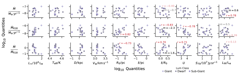
Figure 10: Correlations of derived mass loss rates with star and bow parameters. First row is for mass-loss rate derived using the method of this paper (§ 5.1). Second row is for mass-loss rate derived using the corrected K18 method (§ 5.2). Third row is the ratio of these two methods. Points show 18 of the 20 K18 sources, omitting the two strongest candidates for radiation support. The correlation coefficient, $r$, and linear regression slope, $m$, are shown for selected pairs of interest (fainter text indicates weaker correlations). These were calculated using the Python library function scipy.stats.linregress.

Figure 11: Relative chord length versus shell thickness. The line and gray shading shows the theoretical relation (eq. (19)) for planitude of $\Pi=1.8\pm 0.9$. The short vertical lines at the top of the graph show the chord lengths for each of the 20 K18 sources. The sources with the four smallest and four largest values of $\ell/R_{0}$ are individually labelled. The mean value of $\ell/R_{0}=1.8$ is indicated by a dashed line, which corresponds to $H/R_{0}=0.25$, which is the common value that we use in deriving $\eta$ and therefore $\dot{M}$ by our method. Inset diagram at lower right shows the geometry that leads to eq. (19).

From comparing the two panels in Figure 6 it is clear that there is a broad average agreement between the $\dot{M}$ values from the two methods. Nevertheless, there is considerable disparity for individual sources. Obviously this is to be expected for sources where the $\tau$–$\eta_{\text{sh}}$ method implies radiation support, since the K18 method assumes stellar wind support in all cases, and so has no way of identifying these. However, discrepancies remain even for sources that are well above the diagonal line in Figure 1. This is shown more clearly in Figure 9, where we compare the two mass-loss determinations. Plot symbols are colored according to the physical size of the bow, $R_{0}$, and radiation-support candidates are shown fainter. It is apparent that there is only weak correlation between the two techniques (Pearson correlation coefficient $r=0.67$). Interestingly, the smaller bows (red/orange shading) show much better agreement than the larger bows (yellow shading). The five bows with $R_{0}>$0.4\text{\,}\mathrm{p}\mathrm{c}$$ (339, 344, 369, 381, 382) show a difference of nearly an order of magnitude, in the sense that our method consistently predicts lower mass-loss rates than K18. The error ellipse for the combined observational errors (see Tab. 4 in App. A) is highly elongated along the leading diagonal in Figure 9 due to the fact that most of the observational uncertainties effect both mass-loss methods in a similar way. It is therefore unlikely that observational errors are a significant contribution to the difference in the two $\dot{M}$ methods, which must instead be due to the systematic model uncertainties. These are represented in the figure by the vertical error bars, which show the effect of a factor of three uncertainty in $\eta_{\text{sh}}$ due to variations in shell thickness, dust opacity, and shell gas temperature. It can be seen that systematic errors of this magnitude could indeed account for the observed differences, but the questions remain: which parameter is causing the problem? and can we correct for it?

Although we have seen (Fig. 9) that the mass-loss discrepancy increases with $R_{0}$, it is hard to understand why the physical size per se might cause this. We have therefore looked at the correlations between all of the observed and derived quantities, showing some of the more interesting results in Figure 10. Each row of plots shows the dependence ($y$ axis) of the two different derived mass-loss rates, and their ratio, on different parameters ($x$ axis) of the star (leftmost four columns) and bow shell (remaining six columns). The most significant correlations are marked in red with the value of the Pearson correlation coefficient, $r$ (calculated after taking the log of all quantities). The values shown with dark text have $r^{2}>0.5$, which means that at least 50% of the variance in the $y$ quantity is “explained” by the variance in the $x$ quantity (although this cannot necessarily be taken to imply causation in either direction since it might be due to the fact that both $x$ and $y$ are partially determined by a third quantity, $z$). For some correlations, we also mark the linear regression slope, $m$. Since we are working in logarithmic space, this is equal to the power index in the relation $y\propto x^{m}$. Some selected weaker correlations are also shown (fainter text).

For our $\eta$–$\tau_{\text{sh}}$ mass-loss method (top row) the only significant correlation is a positive one with the shell infrared luminosity $L_{\text{IR}}$ (rightmost column), with slope $m=0.6\pm 0.1$. For the K18 mass-loss method (middle row), the situation is very different, showing significant correlation with a trio of quantities: a positive correlation with bow radius, $R_{0}$, and negative correlations with relative chord length, $\ell/R_{0}$, and radiation field at the shell, $U$. The same three correlations (with inverted sense) are seen for the ratio of the two methods (bottom row). This is due to the fact that the $\eta$–$\tau_{\text{sh}}$ method shows much shallower slopes in its (weak) correlations with these quantities. As an example, we show the values for $\ell/R_{0}$ on the figure (seventh column): $m=-2.3\pm 0.4$ for the K18 method but $m=-0.7\pm 0.4$ for our method, which leaves a significant slope in the ratio of $m=1.6\pm 0.4$. For the shell luminosity, on the other hand, the ratio does not show any significant correlation at all. This is because both methods have essentially the same slope in their correlation with $L_{\text{IR}}$: $m=0.6\pm 0.1$ for our method, and a weak correlation with $m=0.5\pm 0.3$ for the K18 method.

Out of the three quantities, $R_{0}$, $\ell/R_{0}$, and $U$ (which are highly correlated between themselves) we will concentrate on the relative chord length $\ell/R_{0}$ as the most likely culprit for the discrepancy between the two mass-loss estimates. This is because it contains observational information that is used in the K18 method (step K2 of § 5.2), but is not used in the $\tau$–$\eta_{\text{sh}}$ method. The closest equivalent of $\ell$ in our method is the shell thickness, $h_{\text{sh}}$, which enters in step P2 of § 2, but crucially we use a fixed fraction of the bow radius, $h_{\text{sh}}/R_{0}=0.25$, rather than basing it on any observations. In principle, we could derive $h_{\text{sh}}$ from $\ell$ if we knew the radius of curvature of the shell, $R_{\text{c}}$, or equivalently the planitude: $\Pi=R_{\text{c}}/R_{0}$ (Tarango-Yong & Henney, 2018). The idealized geometry is illustrated in the inset to Figure 11, from which we find

$$\frac{h_{\text{sh}}}{R_{0}}=\frac{1}{8\Pi}\left(\frac{\ell}{R_{0}}\right)^{2}\ .$$ (19)

This is plotted in Figure 11 for planitudes of $\Pi=1.8\pm 0.9$, which are typical of OB star bows (this will be shown in detail in the upcoming Paper IV). Also shown in the figure are the individual relative chord lengths for the K18 sources (rug plot at top). Although the mean value of $\ell/R_{0}\approx 1.8$ corresponds closely to the $h_{\text{sh}}/R_{0}=0.25$ that we have used, the sources with $\ell/R_{0}<1$ are predicted to have thinner shells with $h_{\text{sh}}/R_{0}<0.1$. The four sources with the lowest values of $\ell/R_{0}$ are labeled on the figure (369, 339, 382, 344) and these are precisely those sources that show the largest discrepancy between the two mass loss methods (Fig. 9). Using a smaller value of $h_{\text{sh}}$ would increase $\eta_{\text{sh}}$ (eq. [2]) and hence $\dot{M}$ (eq. [17]), thereby reducing the discrepancy between the two methods.

We choose not make this correction to the $\tau$–$\eta_{\text{sh}}$ method in this paper since we want to test the methods using published data alone and without excessive fine-tuning. However, for future applications an empirical measurement of the shell thicknesses would clearly help improve the reliability of the $\tau$–$\eta_{\text{sh}}$ method.

It is hard to say which of the two mass-loss methods is “better”, except that the $\tau$–$\eta_{\text{sh}}$ method has the advantage of being able to identify radiation-supported bows, for which the mass loss cannot be determined. We recommend that both be employed if possible as a cross-check on one another. The $\tau$–$\eta_{\text{sh}}$ method has the disadvantage of requiring shell photometry at a range of wavelengths: $8\text{\,}\mathrm{\SIUnitSymbolMicro m}70\text{\,}\mathrm{\SIUnitSymbolMicro m}$ in order to be sure of covering the bulk of the grain emission, whereas the K18 method needs only the $70\text{\,}\mathrm{\SIUnitSymbolMicro m}$ surface brightness. On the other hand, we suspect that this makes the $\tau$–$\eta_{\text{sh}}$ method less sensitive to possible variations in grain composition and size distribution. This is because it depends on the average grain opacity over a broad range of ultraviolet wavelengths, rather than the emissivity in a single infrared band. Additionally, many bows are weak emitters at $70\text{\,}\mathrm{\SIUnitSymbolMicro m}$, whereas the background emission from the PDRs surrounding H ii regions is very bright and variable. The contrast of the bow against the background is usually much higher at $24\text{\,}\mathrm{\SIUnitSymbolMicro m}$, but K18 avoid this waveband on the grounds that it may be dominated by emission from stochastic heating of very small grains. We maintain that this avoidance is over-conservative (see § 4.1.1), since (i) the high circumstellar radiation fields ($U>1000$) mean that stochastic heating is only relevant for ultra-small nanometer-sized grains (Draine & Li, 2001), and (ii) the most important class of such grains in the general ISM is PAHs, and these are destroyed by the ionizing radiation from O stars (Desert et al., 1990). Although PAHs may survive in bows around B stars, which lack the energetic photons ($h\nu>$40\text{\,}\mathrm{e}\mathrm{V}$$) that most efficiently destroy them (Lebouteiller et al., 2007), their contribution to the $24\text{\,}\mathrm{\SIUnitSymbolMicro m}$ emissivity is likely to be small compared with the slightly larger grains ($>$5\text{\,}\mathrm{n}\mathrm{m}$$), which are in thermal equilibrium with the radiation field. It may therefore be worth modifying the K18 method to use the $24\text{\,}\mathrm{\SIUnitSymbolMicro m}$ surface brightness instead of $70\text{\,}\mathrm{\SIUnitSymbolMicro m}$. In the case of the $\tau$–$\eta_{\text{sh}}$ method, this is all irrelevant since equation (1) is valid in a time-averaged sense, irrespective of whether stochastic heating is important or not.

6.3 Common characteristics of radiation-supported candidates

For five of the K18 sources (380, 407, 409, 410, 411), our method of § 5.1 gives only an upper limit to the wind mass-loss rate if one assumes a factor-three uncertainty in $\eta_{\text{sh}}$, raising the possibility that they may be radiation-supported instead of wind-supported (see Paper I). It is notable that these sources are among the smallest in the K18 sample, all with $R_{0}<$0.1\text{\,}\mathrm{p}\mathrm{c}$$. The two Orion Nebula bows, LP Ori and $\theta^{1}$ Ori D also fall into this category, and they are smaller still, with $R_{0}<$0.01\text{\,}\mathrm{p}\mathrm{c}$$. Six of these 7 stars also occupy a narrow range of spectral type between O9 and B0, corresponding to $T_{\text{eff}}=\text{$28\text{\,}\mathrm{k}\mathrm{K}31\text{\,}\mathrm{k}\mathrm{K}$}$ (LP Ori is a much cooler B2 star with $T_{\text{eff}}=$20\text{\,}\mathrm{k}\mathrm{K}$$, Petit et al., 2008; Alecian et al., 2013).

The small bow sizes are fully consistent with the expectations from the theory developed in Paper I. Radiation-supported bows are predicted to occur either in high-density environments ($n>$100\text{\,}\mathrm{c}\mathrm{m}^{-3}$$) or for stars with particularly weak winds. In either case, the bow is expected to be smaller than $0.1\text{\,}\mathrm{p}\mathrm{c}$ for $v_{\infty}\geq$20\text{\,}\mathrm{k}\mathrm{m}\,\mathrm{s}^{-1}$$, see Figures 2a,b and 8 of Paper I.

Another common property of these sources is that they all have high ratios of chord length to stand-off radius, $\ell/R_{0}$. For instance, from Figure 11, the four sources with the highest $\ell/R_{0}$ values are all among the five radiation-supported candidates. From equation (19) this means they also should have thicker than average shells. This is consistent with our finding from Paper I’s § 3.3 that the shell tends to be broad in the radiation-supported bow wave regime. Furthermore, if the larger than average $H/R_{0}$ were to be taken account in the calculation of $\eta_{\text{sh}}$ (eq. [2]), then it would strengthen the case for radiation support in these objects.

6.4 The anomalous B star KGK2010 2 in Cygnus: strong wind or trapped ionization front?

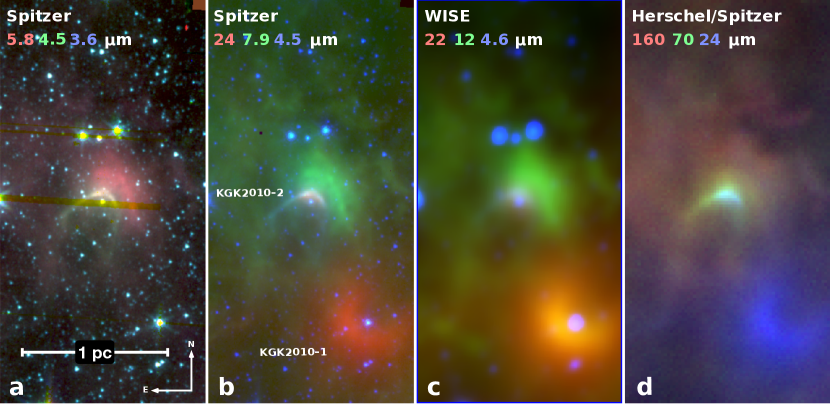
Figure 12: Two neighboring but highly contrasting bows in Cygnus: KGK2010 2 (source 342) and KGK2010 1 (source 341). Each panel shows the same $3.6^{\prime}\times 7.4^{\prime}$ field, centered on equatorial coordinates $(\alpha,\delta)=20^{\text{h}}34^{\text{m}}34.50^{\text{s}},$$$, but in different combinations of three filters, as marked.

K18 source 342 is the only source that shows a significant discrepancy above the theoretical mass-loss rate predictions. This is bow shock candidate 2 in a survey of mid-infrared arcs in Cygnus X (Kobulnicky et al., 2010), and is referred to as KGK2010 2 in subsequent works. For its early B spectral type, $\dot{M}\approx$3\text{\times}{10}^{-9}\text{\,}\mathrm{M}_{\odot}\,\mathrm{y}\mathrm{r}^{-1}$$ is expected, whereas the derived values from both mass-loss methods (panels a and b of Fig. 6) are about 10 times larger. This fact was already noted in K18, who suggested that the grain emissivity models may not be appropriate for this object. We propose instead to investigate the idea that the shell may be predominantly neutral instead of ionized, which might help explain other peculiar aspects of the source. Figure 12 shows infrared images of the field containing both sources 342 and 341. The field is located in the Cygnus X North region, between the DR 20 and DR 21 star forming regions, about $17\text{\,}\mathrm{p}\mathrm{c}$ north of the center of the Cygnus OB2 association (e.g., Schneider et al., 2016). It can be seen that the two bow shocks have very contrasting morphologies and spectra. Source 341 has a semi-circular shape, a very diffuse outer boundary, and is only prominent between wavelengths of $12\text{\,}\mathrm{\SIUnitSymbolMicro m}$ and $24\text{\,}\mathrm{\SIUnitSymbolMicro m}$. These characteristics are typical of many optically thin bows seen in fully ionized gas, such as the Ney–Allen nebula around $\theta^{1}$ Ori D compare the bow shape in Fig. 3a of Smith et al., 2005, source 406 HD 92607, which is ERO 36 in Carina, Sexton et al., 2015, and the central star of RCW 120 not included in current samples, but see Mackey et al., 2015, 2016. Source 342, on the other hand, has a more parabolic shape, a sharply defined outer boundary to its arc, and emits strongly at all wavelengths from $3.6\text{\,}\mathrm{\SIUnitSymbolMicro m}$ to $150\text{\,}\mathrm{\SIUnitSymbolMicro m}$ see also Fig. 13 of Kobulnicky et al., 2010. The parabolic arc shape and the broad SED are both reminiscent of LP Ori (more details on the Orion Nebula bows will be provided in Paper VI), and another bow that bears some similarities is Carina’s Sickle object ERO 21 Sexton et al., 2015, see also Ngoumou et al., 2013 and § 4 of Hartigan et al., 2015. Note also the second outer rim in this source, which emits primarily at $5.8\text{\,}\mathrm{\SIUnitSymbolMicro m}$, $7.9\text{\,}\mathrm{\SIUnitSymbolMicro m}$, and $12\text{\,}\mathrm{\SIUnitSymbolMicro m}$. This appears similar to the double-bow structure seen in IRAS 03063+5735 (Kobulnicky et al., 2012). Finally, it has the coldest dust of any of the K18 sources, as determined from the mid-to-far infrared color temperatures ($T_{22/70}=$70\text{\,}\mathrm{K}$$, $T_{70/150}=$69\text{\,}\mathrm{K}$$ from Tab. 5 of Kobulnicky et al., 2017).

If source 342 has trapped the ionization front in its shell, then $\eta_{\text{sh}}$ has been overestimated and the source should be moved vertically down on Figure 1 in a similar way to LP Ori. The exact correction factor is unknown, since it depends on the temperature and magnetic field in the neutral shell, but it could easily be of order 10, which would take the shell into the radiation-supported regime. The derived mass-loss rate would hence be reduced from the anomalously high value of Figure 9 to essentially zero. However, this requires that the shell be capable of absorbing all the ionizing photons from the central star, which implies a lower limit to the shell optical depth: $\tau>\tau_{\text{trap}}$, see Paper I’s § 3.1. In the radiation-supported bow wave (RBW) regime this is

$$\text{RBW:}\quad\tau_{\text{trap}}\approx 7.1\,\left(\frac{S_{49}\,\kappa_{600}}{L_{4}}\right)^{1/2}\ ,$$ (20)

while in the wind-supported bow shock (WBS) regime it is

$$\text{WBS:}\quad\tau_{\text{trap}}\approx 102\,\frac{S_{49}\,\kappa_{600}}{\eta_{\text{w}}\,L_{4}}\ .$$ (21)

In these equations, which are derived from equations (8, 10, 12, 24) of Paper I, $S_{49}$ is the ionizing photon luminosity of the star in units of ${10}^{49}\text{\,}\mathrm{s}^{-1}$, while $L_{4}$ and $\kappa_{600}$ are defined in § 2 and $\eta_{\text{w}}$ in § 5.1. Within the uncertainties, the observationally inferred spectral type of B0–B2V of source 342 is the same as the $10\text{\,}\mathrm{M}_{\odot}$ main-sequence star used in Papers I and II, which has a ratio of ionizing to bolometric luminosity $S_{49}/L_{4}=$2.1\text{\times}{10}^{-4}$$. Substituting into equation (20) yields $\tau_{\text{trap}}\approx 0.1$ for the RBW case, whereas the observed optical depth is more than an order of magnitude lower: $\tau\approx 0.005$. Similar difficulties arise if one assumes a wind-supported bow shock, in which case $\tau<\eta_{\text{w}}$ by definition. Combined with equation (21), this then implies a lower limit for the wind momentum efficiency: $\eta_{\text{w}}>0.14$. Given that we must always have $\eta_{\text{sh}}\geq\eta_{\text{w}}$ (eq. [15]), this is inconsistent with the observed $\eta_{\text{sh}}=0.07T_{4}/\kappa_{600}h_{1/4}$, especially since the whole point of the exercise is to reduce $\eta_{\text{sh}}$ via a reduction in $T_{4}$.

Therefore, we have shown that source 342 cannot have a neutral shell if we take the published observational data at face value. However, more recent spectroscopic observations revise the spectral classification to B4 V (H. Kobulnicky, priv. comm.) and this would change the picture completely. A B4 dwarf, with effective temperature of $16\,700\text{\,}\mathrm{K}$ (Tab. 4 of Pecaut & Mamajek, 2013) would have a very small ionizing luminosity. Interpolating on Table 4 of Lanz & Hubeny (2007), we find $S_{49}/L_{4}\approx$4\text{\times}{10}^{-6}$$, which yields $\tau_{\text{trap}}=0.017$ from equation (20). At the same time, the revised spectroscopy implies a smaller $L_{*}$ by roughly a factor of 10, which increases the shell’s derived $\tau$ by the same factor (eq. [1]), yielding $\tau\approx 0.05$. Since we now have $\tau>\tau_{\text{trap}}$ it is possible that ionization front may be trapped, giving a predominately neutral shell. This also relies, however, on the radiation field from the nearby Cygnus OB2 cluster being insufficient to ionize the shell. Given that the cluster’s stellar population (Wright et al., 2015) includes 3 WR stars and a handful of early-O supergiants, the ionizing luminosity must be of order ${10}^{51}\text{\,}\mathrm{s}^{-1}$. In the absence of absorption, and assuming that the true separation be no more than a few times larger than the projected separation, the cluster stars would contribute over 100 times greater ionizing flux at the position of source 342 than that due to the B4 star itself. It is therefore necessary for the source to lie outside of the cluster’s H ii region in order for the shell to be neutral. It is quite plausible that this might be the case, since radio continuum observations Fig. 4 of Wendker et al., 1991 and Fig. 7 of Tung et al., 2017 indicate that the neighborhood of source 342 is a local minimum in free-free emission between discrete H ii regions of the Cygnus X complex, while Herschel maps (Schneider et al., 2016) show the presence of both warm and cold dust along the line of sight and clumps of Class 0 and I YSOs are seen nearby (Beerer et al., 2010), indicative of shielded neutral/molecular gas.

7 Summary

We have proposed a novel diagnostic method, the $\tau$-$\eta_{\text{sh}}$ diagram, for analyzing observations of stellar bow shocks around OB stars, which allows discrimination between radiation-supported and wind-supported bows. Our principal results are as follows:

1. The UV optical depth $\tau$ of the bow shell can be estimated from the observed infrared shell luminosity $L_{\text{IR}}$ and stellar luminosity $L_{*}$ as $\tau=2L_{\text{IR}}/L_{*}$ (§ 2).

2. The shell momentum efficiency $\eta_{\text{sh}}$, which is the fraction of stellar radiative momentum that is transferred to the shell either directly or indirectly (via stellar wind), can be estimated from $\tau$ and the observed shell radius $R_{0}$, after making some auxiliary assumptions about the physical conditions in the shell (§ 2).

3. By comparing $\tau$ and $\eta_{\text{sh}}$, it is possible to discriminate between three regimes (§ 3 and see Paper I): wind-supported bow shocks ($\eta_{\text{sh}}\gg\tau$), radiation-supported bow waves ($\eta_{\text{sh}}\sim\tau<1$), and radiation-supported bow shocks ($\eta_{\text{sh}}\sim\tau>1$).

4. Shells with $\eta_{\text{sh}}<${10}^{-3}$$ are potentially in a fourth regime of dust waves, where gas–grain collisional coupling breaks down (see Paper II).

5. By analyzing a published sample of 20 mid-infrared bow shock candidates (Kobulnicky et al., 2018, K18), plus additional compact bows in Orion, we find 4 strong candidates for radiation-supported bow waves plus 3 marginal cases (§§ 3.5 and 6.3). No strong candidates for dust waves are found.

6. For wind-supported bow shocks, the stellar wind mass-loss rate can be found from $\tau$ and $\eta_{\text{sh}}$ (§ 5.1). We compare this method with the previously proposed method of K18 (§ 5.2) and suggest a correction to the dust emissivities used in the latter, which reduces the mass-loss rates by a factor of about 2.

7. After this correction, the two mass-loss methods agree well for small bows ($R_{0}\leq$0.3\text{\,}\mathrm{p}\mathrm{c}$$), but the $\tau$–$\eta_{\text{sh}}$ method under-predicts the mass-loss rate by up to a factor of 10 for larger bows, which also tend to have relatively thin shells (§ 6.2). This discrepancy could be eliminated by extending the $\tau$–$\eta_{\text{sh}}$ method to include the observed shell thickness.

8. Disruption of the largest dust grains by rotational torques in the strong circumstellar radiation field is predicted to increase the UV opacity by about 50% (§ 6.1), although the effect could be larger if the resulting fragments are very small.

9. The bow source KGK2010 2 is a low-luminosity B star with an anomalously high apparent mass-loss rate. This discrepancy could be eliminated if the bow shell has trapped the ionization front and is predominantly neutral, in which case it would become yet another candidate for radiation support.

Appendix A Covariance of derived quantities from propagation of observational uncertainties

Table 2: Propagation of observational uncertainties to derived quantities

$x_{i}$	$\sigma_{x_{i}}$	$J_{x_{i}}(\tau)$	$J_{x_{i}}(\eta_{\text{sh}})$	$J_{x_{i}}(\dot{M})$	$J_{x_{i}}(\dot{M}_{\text{K18}})$	$J_{x_{i}}(L_{*})$
$D$	$0.08$	$2$	$3$	$3$	$2$	$0$
$L_{*}$	$0.18$	$-1$	$-2$	$-1$	$-0.5$	$1$
$F_{\text{IR}}$	$0.12$	$1$	$1$	$1$	$0$	$0$
$I_{70}$	$0.12$	$0$	$0$	$0$	$1$	$0$
$\theta$	$0.11$	$0$	$1$	$1$	$2$	$0$
$\ell/R$	$0.08$	$0$	$0$	$0$	$-1$	$0$
$V_{\text{w}}$	$0.18$	$0$	$0$	$-1$	$-1$	$0$

Even though errors in the fundamental observed quantities, $x_{i}$, are assumed independent, errors in the derived quantities, $f_{k}(x_{1},x_{2},\dots)$, will not necessarily be so. For the purposes of this paper:

$$x_{i}\in \left\{D;\ L_{*};\ F_{\text{IR}};\ I_{70};\ \theta;\ \ell/R;\ V_{\text{w}}\right\}$$ (22)

$$f_{k}\in \left\{\tau;\ \eta_{\text{sh}};\ \dot{M};\ \dot{M}_{\text{K18}};\ L_{*}\right\}\ .$$ (23)

Note that $L_{*}$ appears in both lists because we use it as a graph axis in Figure 6. For the case where each $f_{k}$ is a simple product of powers of the $x_{i}$, the propagation of errors reduces to linear algebra of log quantities. This is exactly true for $\tau$ and $\eta_{\text{sh}}$, but only approximately so for $\dot{M}$ and $\dot{M}_{\text{K18}}$. We define $J_{x_{i}}(f_{k})$ as the elements of the Jacobian matrix of logarithmic derivatives $d\ln f_{k}/d\ln x_{i}$, which are given for our quantities in Table 2. Then, the elements of the variance–covariance matrix for the derived parameters are

$$C_{k,k^{\prime}}=\sum_{i}J_{x_{i}}(f_{k})\,\sigma_{x_{i}}^{2}\,J_{x_{i}}(f_{k^{\prime}})\ ,$$ (24)

where the $\sigma_{x_{i}}$ are the rms dispersions in $x_{i}$, measured in dex. In Figure 13 we give example python code for calculating this matrix, using the $\sigma_{x_{i}}$ derived in § 3.2.1–3.2.5 for the K18 sources (second column of Tab. 2), with results given in Table 3. It can be seen that many of the off-diagonal elements are of similar magnitude to the diagonal elements, which is an indication of significant correlations between the errors in the different parameters.

Table 3: Variance–covariance matrix $C_{k,k^{\prime}}$ for derived quantities

	$\tau$	$\eta_{\text{sh}}$	$\dot{M}$	$\dot{M}_{\text{K18}}$	$L_{*}$
$\tau$	$0.0724$	$0.1176$	$0.0852$	$0.0418$	$-0.0324$
$\eta_{\text{sh}}$	$0.1176$	$0.2137$	$0.1489$	$0.095$	$-0.0648$
$\dot{M}$	$0.0852$	$0.1489$	$0.1489$	$0.1112$	$-0.0324$
$\dot{M}_{\text{K18}}$	$0.0418$	$0.095$	$0.1112$	$0.1353$	$-0.0162$
$L_{*}$	$-0.0324$	$-0.0648$	$-0.0324$	$-0.0162$	$0.0324$

For any particular pair of derived quantities, $f_{m}$ and $f_{n}$, one can find the error ellipse that characterises the projection of observational errors onto the $f_{m}$–$f_{n}$ plane. The ellipse is characterized by standard deviations along major and minor axes, $\sigma_{a}$, $\sigma_{b}$, together with the angle $\theta_{a}$ between the $f_{m}$ axis and the ellipse major axis. These are given via the eigenvalues and eigenvectors of the relevant $2\times 2$ submatrix of the covariance matrix:

$$\sigma_{a}^{2}= \frac{1}{2}\left\{C_{m,m}+C_{n,n}+\left[\left(C_{m,m}+C_{n,n}\right)^{2}-4C_{m,n}^{2}\right]^{1/2}\right\}$$ (25)

$$\sigma_{b}^{2}= \frac{1}{2}\left\{C_{m,m}+C_{n,n}-\left[\left(C_{m,m}+C_{n,n}\right)^{2}-4C_{m,n}^{2}\right]^{1/2}\right\}$$ (26)

$$\theta_{a}= \frac{1}{2}\arctan\left(\frac{2C_{m,n}}{C_{m,m}-C_{n,n}}\right)\ .$$ (27)

For instance, Table 4 shows the resultant error ellipse parameters (shown in blue on the respective graphs) for the relations plotted in Figures 1, 6ab, and 9.

Table 4: Error ellipse parameters for particular pairs of derived quantities

$f_{m}$	$f_{n}$	$\sigma_{a}$	$\sigma_{b}$	$\theta_{a}$, $\mathrm{\SIUnitSymbolDegree}$	Figure
$\tau$	$\eta$	$0.529$	$0.077$	$60.5$	1
$L_{*}$	$\dot{M}$	$0.397$	$0.155$	$-75.5$	6a
$L_{*}$	$\dot{M}_{\text{K18}}$	$0.371$	$0.173$	$-81.3$	6b
$\dot{M}_{\text{K18}}$	$\dot{M}$	$0.503$	$0.175$	$46.7$	9

import numpy as np
sig = np.diag([0.08, 0.18, 0.12, 0.12, 0.11, 0.08, 0.18])
J = np.array([
    [2, -1, 1, 0, 0, 0, 0],
    [3, -2, 1, 0, 1, 0, 0],
    [3, -1, 1, 0, 1, 0, -1],
    [2, -0.5, 0, 1, 2, -1, -1],
    [0, 1, 0, 0, 0, 0, 0]
])
C = J @ sig**2 @ J.T
  

Figure 13: Snippet of Python code that calculates the covariance matrix of Table 3. The last line implements equation (24) by a triple matrix product of the Jacobian matrix J, the square of a diagonal matrix of observational standard deviations sig, and the transpose of J.

Appendix B The Herbig Be star V750 Mon

K18 source 380 (HD 53367, V750 Mon) is a Herbig Be star with spectral type B0V–B0III and mass 12 to $15\text{\,}\mathrm{M}_{\odot}$, which shows long-scale irregular photometric variability (Tjin A Djie et al., 2001; Pogodin et al., 2006) together with cyclic radial velocity variations, which are interpreted as an eccentric binary with a $5\text{\,}\mathrm{M}_{\odot}$ pre-main-sequence companion. It is located outside the solar circle and, although it was originally classified as part of the CMa OB association at about $1\text{\,}\mathrm{k}\mathrm{p}\mathrm{c}$ (Tjin A Djie et al., 2001), more recent estimates put it much closer. K18 assume a distance of $260\text{\,}\mathrm{p}\mathrm{c}$, based on Hipparcos measurements (van Leeuwen, 2007), but its Gaia DR2 parallax (Gaia Collaboration et al., 2016, 2018; Luri et al., 2018) puts it closer still at $140\pm 30\text{\,}\mathrm{p}\mathrm{c}$. This is the median and 90% confidence interval, estimated from Bayesian inference using an exponential density distribution with scale length of $1350\text{\,}\mathrm{p}\mathrm{c}$ as a prior.

Quireza et al. (2006b) report a kinematic distance to the associated H ii region IC 2177 (G$223.70$$-1.90$) of $1.6\text{\,}\mathrm{k}\mathrm{p}\mathrm{c}$, based an LSR radio recombination line velocity of $16\text{\,}\mathrm{k}\mathrm{m}\,\mathrm{s}^{-1}$ (Quireza et al., 2006a) and the outer Galaxy rotation curve of Brand & Blitz (1993). However, given the dispersion in peculiar velocities of star-forming clouds ($7\text{\,}\mathrm{k}\mathrm{m}\,\mathrm{s}^{-1}9\text{\,}\mathrm{k}\mathrm{m}\,\mathrm{s}^{-1}$, Stark, 1984) and likely streaming motions of the ionized gas ($\approx$10\text{\,}\mathrm{k}\mathrm{m}\,\mathrm{s}^{-1}$$, Matzner, 2002; Lee et al., 2012), this is still consistent with a much smaller distance, which would also help in bringing the radio continuum-derived nebular electron density into agreement with the value ($\approx$100\text{\,}\mathrm{c}\mathrm{m}^{-3}$$) derived from the optical [S ii] line ratio (Hawley, 1978).

Fairlamb et al. (2015) derive a distance of $340\pm 60\text{\,}\mathrm{p}\mathrm{c}$ from combining a spectroscopically determined effective temperature, gravity, and reddening with photometry and pre-main sequence evolutionary tracks. They also determine a luminosity of $13\,000\pm 1000\text{\,}\mathrm{L}_{\odot}$, which is only half that assumed by K18, and would have to be even lower to bring the photometry into concordance with the Gaia distance. Alternatively, the luminosity could remain the same if the total-to-selective extinction ratio were higher than the $R_{V}=3.1$ assumed by Fairlamb et al. (2015). Taking $R_{V}=5.5$ instead, as in Orion, would give $A_{V}=3.34$ and a predicted $V$ magnitude of 6.7 if we assume $L_{4}=1.3$, $D=$170\text{\,}\mathrm{p}\mathrm{c}$$ (furthest distance in Gaia 90% confidence interval) and $T_{\text{eff}}=$29.5\text{\,}\mathrm{k}\mathrm{K}$$ (Fairlamb et al., 2015) for a bolometric correction of $-2.86$ (Nieva, 2013). The observed brightness varies between $V=6.9$ and 7.2, which is still at least 20% fainter than predicted, but this is the best that can be achieved without rejecting the Gaia parallax distance entirely.

A final sanity check can be performed by considering the free-free radio continuum flux of V750 Mon’s surrounding H ii region, which, after converting to a luminosity, should be proportional to the total recombination rate in the nebula and therefore, assuming photoionization equilibrium and negligible dust absorption in the ionized gas, also proportional to the ionizing photon luminosity of the star. Quireza et al. (2006b) report a flux density of $6\text{\,}\mathrm{J}\mathrm{y}$ at $8.6\text{\,}\mathrm{G}\mathrm{h}\mathrm{z}$ for G$223.70$$-1.90$, as compared with a flux density of $260\text{\,}\mathrm{J}\mathrm{y}$ for the Orion Nebula using the same instrumental setup. Assuming an ionizing photon luminosity of $S_{49}=1$ and distance $410\text{\,}\mathrm{p}\mathrm{c}$ for the ionizing Trapezium stars in Orion, therefore implies $S_{49}=0.0027(D/$140\text{\,}\mathrm{p}\mathrm{c}$)^{2}$ for V750 Mon. Using an ionizing flux of $3.2\text{\times}{10}^{22}\text{\,}\mathrm{c}\mathrm{m}^{-2}\,\mathrm{s}^{-1}$ from the curves in Fig. 4 of Sternberg et al. (2003), this translates to a bolometric luminosity of $L_{4}=0.96(D/$140\text{\,}\mathrm{p}\mathrm{c}$)^{2}$, which is consistent with the Fairlamb et al. (2015) value if we take a distance towards the high end of the Gaia range.

References

- Acreman et al. (2016) Acreman D. M., Stevens I. R., Harries T. J., 2016, MNRAS, 456, 136
- Alecian et al. (2013) Alecian E., et al., 2013, MNRAS, 429, 1001
- Arthur & Hoare (2006) Arthur S. J., Hoare M. G., 2006, ApJS, 165, 283
- Arthur et al. (2011) Arthur S. J., Henney W. J., Mellema G., de Colle F., Vázquez-Semadeni E., 2011, MNRAS, 414, 1747
- Astropy Collaboration et al. (2013) Astropy Collaboration et al., 2013, A&A, 558, A33
- Astropy Collaboration et al. (2018) Astropy Collaboration et al., 2018, AJ, 156, 123
- Balog et al. (2014) Balog Z., et al., 2014, Experimental Astronomy, 37, 129
- Beerer et al. (2010) Beerer I. M., et al., 2010, ApJ, 720, 679
- Beitia-Antero & Gómez de Castro (2017) Beitia-Antero L., Gómez de Castro A. I., 2017, MNRAS, 469, 2531
- Blaauw (1961) Blaauw A., 1961, Bull. Astron. Inst. Netherlands, 15, 265
- Bodensteiner et al. (2018) Bodensteiner J., Baade D., Greiner J., Langer N., 2018, A&A, 618, A110
- Brand & Blitz (1993) Brand J., Blitz L., 1993, A&A, 275, 67
- Brown (2015) Brown W. R., 2015, ARA&A, 53, 15
- Callingham et al. (2019) Callingham J. R., Tuthill P. G., Pope B. J. S., Williams P. M., Crowther P. A., Edwards M., Norris B., Kedziora-Chudczer L., 2019, Nature Astronomy, 3, 82
- Canto et al. (1996) Canto J., Raga A. C., Wilkin F. P., 1996, ApJ, 469, 729
- Cantó et al. (2005) Cantó J., Raga A. C., González R., 2005, Rev. Mex. Astron. Astrofis., 41, 101
- Comeron & Kaper (1998) Comeron F., Kaper L., 1998, A&A, 338, 273
- Cordes et al. (1993) Cordes J. M., Romani R. W., Lundgren S. C., 1993, Nature, 362, 133
- Cox et al. (2012) Cox N. L. J., et al., 2012, A&A, 537, A35
- Desert et al. (1990) Desert F.-X., Boulanger F., Puget J. L., 1990, A&A, 237, 215
- Draine (1981) Draine B. T., 1981, ApJ, 245, 880
- Draine & Li (2001) Draine B. T., Li A., 2001, ApJ, 551, 807
- Draine & Li (2007) Draine B. T., Li A., 2007, ApJ, 657, 810
- Duley (1973) Duley W. W., 1973, Ap&SS, 23, 43
- Engelbracht et al. (2007) Engelbracht C. W., et al., 2007, PASP, 119, 994
- Fairlamb et al. (2015) Fairlamb J. R., Oudmaijer R. D., Mendigutía I., Ilee J. D., van den Ancker M. E., 2015, MNRAS, 453, 976
- Ferland et al. (2013) Ferland G. J., et al., 2013, Rev. Mex. Astron. Astrofis., 49, 137
- Ferland et al. (2017) Ferland G. J., et al., 2017, Rev. Mex. Astron. Astrofis., 53, 385
- Fitzpatrick & Massa (2007) Fitzpatrick E. L., Massa D., 2007, ApJ, 663, 320
- Gaia Collaboration et al. (2016) Gaia Collaboration et al., 2016, A&A, 595, A1
- Gaia Collaboration et al. (2018) Gaia Collaboration et al., 2018, A&A, 616, A1
- Giard et al. (1994) Giard M., Bernard J. P., Lacombe F., Normand P., Rouan D., 1994, A&A, 291, 239
- Gull & Sofia (1979) Gull T. R., Sofia S., 1979, ApJ, 230, 782
- Gvaramadze et al. (2012) Gvaramadze V. V., Langer N., Mackey J., 2012, MNRAS, 427, L50
- Gvaramadze et al. (2018) Gvaramadze V. V., Alexashov D. B., Katushkina O. A., Kniazev A. Y., 2018, MNRAS, 474, 4421
- Habing (1968) Habing H. J., 1968, Bull. Astron. Inst. Netherlands, 19, 421
- Hartigan et al. (2015) Hartigan P., Reiter M., Smith N., Bally J., 2015, AJ, 149, 101
- Hawley (1978) Hawley S. A., 1978, ApJ, 224, 417
- Henney (2002) Henney W. J., 2002, Revista Mexicana de Astronomia y Astrofisica, 38, 71
- Henney & Arthur (1998) Henney W. J., Arthur S. J., 1998, AJ, 116, 322
- Henney & Arthur (2019a) Henney W. J., Arthur S. J., 2019a, arXiv e-prints, 1903.03737 MNRAS submitted (Paper I)
- Henney & Arthur (2019b) Henney W. J., Arthur S. J., 2019b, arXiv e-prints, 1903.07774 MNRAS submitted (Paper II)
- Hirabayashi (2015) Hirabayashi M., 2015, MNRAS, 454, 2249
- Hoang et al. (2018) Hoang T., Tram L. N., Lee H., Ahn S.-H., 2018, arXiv, 1810.05557
- Hoogerwerf et al. (2001) Hoogerwerf R., de Bruijne J. H. J., de Zeeuw P. T., 2001, A&A, 365, 49
- Huthoff & Kaper (2002) Huthoff F., Kaper L., 2002, A&A, 383, 999
- Jewitt et al. (2014) Jewitt D., Agarwal J., Li J., Weaver H., Mutchler M., Larson S., 2014, ApJ, 784, L8
- Jones et al. (2019) Jones E., Oliphant T., Peterson P., et al., 2001–2019, SciPy: Open source scientific tools for Python, http://www.scipy.org/
- Katushkina et al. (2017) Katushkina O. A., Alexashov D. B., Izmodenov V. V., Gvaramadze V. V., 2017, MNRAS, 465, 1573
- Katushkina et al. (2018) Katushkina O. A., Alexashov D. B., Gvaramadze V. V., Izmodenov V. V., 2018, MNRAS, 473, 1576
- Kobulnicky et al. (2010) Kobulnicky H. A., Gilbert I. J., Kiminki D. C., 2010, ApJ, 710, 549
- Kobulnicky et al. (2012) Kobulnicky H. A., Lundquist M. J., Bhattacharjee A., Kerton C. R., 2012, AJ, 143, 71
- Kobulnicky et al. (2016) Kobulnicky H. A., et al., 2016, ApJS, 227, 18
- Kobulnicky et al. (2017) Kobulnicky H. A., Schurhammer D. P., Baldwin D. J., Chick W. T., Dixon D. M., Lee D., Povich M. S., 2017, AJ, 154, 201
- Kobulnicky et al. (2018) Kobulnicky H. A., Chick W. T., Povich M. S., 2018, ApJ, 856, 74 (K18)
- Krtička (2014) Krtička J., 2014, A&A, 564, A70
- Krtička & Kubát (2017) Krtička J., Kubát J., 2017, A&A, 606, A31
- Lanz & Hubeny (2007) Lanz T., Hubeny I., 2007, ApJS, 169, 83
- Lebouteiller et al. (2007) Lebouteiller V., Brandl B., Bernard-Salas J., Devost D., Houck J. R., 2007, ApJ, 665, 390
- Lebouteiller et al. (2011) Lebouteiller V., Bernard-Salas J., Whelan D. G., Brandl B., Galliano F., Charmandaris V., Madden S., Kunth D., 2011, ApJ, 728, 45
- Lee et al. (2012) Lee E. J., Murray N., Rahman M., 2012, ApJ, 752, 146
- Luri et al. (2018) Luri X., et al., 2018, A&A, 616, A9
- Mackey et al. (2015) Mackey J., Gvaramadze V. V., Mohamed S., Langer N., 2015, A&A, 573, A10
- Mackey et al. (2016) Mackey J., Haworth T. J., Gvaramadze V. V., Mohamed S., Langer N., Harries T. J., 2016, A&A, 586, A114
- Marcolino et al. (2009) Marcolino W. L. F., Bouret J.-C., Martins F., Hillier D. J., Lanz T., Escolano C., 2009, A&A, 498, 837
- Martins et al. (2005) Martins F., Schaerer D., Hillier D. J., 2005, A&A, 436, 1049
- Mathis et al. (1983) Mathis J. S., Mezger P. G., Panagia N., 1983, A&A, 128, 212
- Matsuda et al. (1989) Matsuda T., Fujimoto Y., Shima E., Sawada K., Inaguchi T., 1989, Progress of Theoretical Physics, 81, 810
- Matzner (2002) Matzner C. D., 2002, ApJ, 566, 302
- McKinney (2010) McKinney W., 2010, in van der Walt S., Millman J., eds, Proceedings of the 9th Python in Science Conference. pp 51 – 56
- Meyer et al. (2014) Meyer D. M.-A., Mackey J., Langer N., Gvaramadze V. V., Mignone A., Izzard R. G., Kaper L., 2014, MNRAS, 444, 2754
- Meyer et al. (2016) Meyer D. M.-A., van Marle A.-J., Kuiper R., Kley W., 2016, MNRAS, 459, 1146
- Meyer et al. (2017) Meyer D. M.-A., Mignone A., Kuiper R., Raga A. C., Kley W., 2017, MNRAS, 464, 3229
- Najarro et al. (2011) Najarro F., Hanson M. M., Puls J., 2011, A&A, 535, A32
- Ngoumou et al. (2013) Ngoumou J., Preibisch T., Ratzka T., Burkert A., 2013, ApJ, 769, 139
- Nieva (2013) Nieva M.-F., 2013, A&A, 550, A26
- O’Dell (2001) O’Dell C. R., 2001, AJ, 122, 2662
- Ochsendorf & Tielens (2015) Ochsendorf B. B., Tielens A. G. G. M., 2015, A&A, 576, A2
- Ochsendorf et al. (2014) Ochsendorf B. B., Cox N. L. J., Krijt S., Salgado F., Berné O., Bernard J. P., Kaper L., Tielens A. G. G. M., 2014, A&A, 563, A65
- Pecaut & Mamajek (2013) Pecaut M. J., Mamajek E. E., 2013, ApJS, 208, 9
- Peri et al. (2012) Peri C. S., Benaglia P., Brookes D. P., Stevens I. R., Isequilla N. L., 2012, A&A, 538, A108
- Peri et al. (2015) Peri C. S., Benaglia P., Isequilla N. L., 2015, A&A, 578, A45
- Petit et al. (2008) Petit V., Wade G. A., Drissen L., Montmerle T., Alecian E., 2008, MNRAS, 387, L23
- Planck Collaboration et al. (2016) Planck Collaboration et al., 2016, A&A, 586, A137
- Pogodin et al. (2006) Pogodin M. A., Malanushenko V. P., Kozlova O. V., Tarasova T. N., Franco G. A. P., 2006, A&A, 452, 551
- Povich et al. (2008) Povich M. S., Benjamin R. A., Whitney B. A., Babler B. L., Indebetouw R., Meade M. R., Churchwell E., 2008, ApJ, 689, 242
- Prišegen (2019) Prišegen M., 2019, A&A, 621, A37
- Quireza et al. (2006a) Quireza C., Rood R. T., Balser D. S., Bania T. M., 2006a, ApJS, 165, 338
- Quireza et al. (2006b) Quireza C., Rood R. T., Bania T. M., Balser D. S., Maciel W. J., 2006b, ApJ, 653, 1226
- Raga et al. (1997) Raga A. C., Noriega-Crespo A., Cantó J., Steffen W., van Buren D., Mellema G., Lundqvist P., 1997, Rev. Mex. Astron. Astrofis., 33, 73
- Robberto et al. (2005) Robberto M., et al., 2005, AJ, 129, 1534
- Salgado et al. (2012) Salgado F., et al., 2012, ApJ, 749, L21
- Salgado et al. (2016) Salgado F., Berné O., Adams J. D., Herter T. L., Keller L. D., Tielens A. G. G. M., 2016, ApJ, 830, 118
- Schlafly et al. (2016) Schlafly E. F., et al., 2016, ApJ, 821, 78
- Schneider et al. (2016) Schneider N., et al., 2016, A&A, 591, A40
- Sexton et al. (2015) Sexton R. O., Povich M. S., Smith N., Babler B. L., Meade M. R., Rudolph A. L., 2015, MNRAS, 446, 1047
- Simón-Díaz et al. (2015) Simón-Díaz S., et al., 2015, ApJ, 799, 169
- Smith et al. (2005) Smith N., Bally J., Shuping R. Y., Morris M., Kassis M., 2005, AJ, 130, 1763
- Spitzer (1978) Spitzer L., 1978, Physical processes in the interstellar medium. New York: Wiley-Interscience
- Stark (1984) Stark A. A., 1984, ApJ, 281, 624
- Sternberg et al. (2003) Sternberg A., Hoffmann T. L., Pauldrach A. W. A., 2003, ApJ, 599, 1333
- Tarango-Yong & Henney (2018) Tarango-Yong J. A., Henney W. J., 2018, MNRAS, 477, 2431
- Tielens & Hollenbach (1985) Tielens A. G. G. M., Hollenbach D., 1985, ApJ, 291, 722
- Tjin A Djie et al. (2001) Tjin A Djie H. R. E., van den Ancker M. E., Blondel P. F. C., Shevchenko V. S., Ezhkova O. V., de Winter D., Grankin K. N., 2001, MNRAS, 325, 1441
- Tung et al. (2017) Tung A. K., et al., 2017, AJ, 154, 156
- Tuthill et al. (1999) Tuthill P. G., Monnier J. D., Danchi W. C., 1999, Nature, 398, 487
- Vink et al. (2000) Vink J. S., de Koter A., Lamers H. J. G. L. M., 2000, A&A, 362, 295
- Weingartner & Draine (2001) Weingartner J. C., Draine B. T., 2001, ApJ, 548, 296
- Wendker et al. (1991) Wendker H. J., Higgs L. A., Landecker T. L., 1991, A&A, 241, 551
- Wilkin (1996) Wilkin F. P., 1996, ApJ, 459, L31
- Wilkin (2000) Wilkin F. P., 2000, ApJ, 532, 400
- Wright et al. (2015) Wright N. J., Drew J. E., Mohr-Smith M., 2015, MNRAS, 449, 741
- Xie et al. (2018) Xie Y., Ho L. C., Li A., Shangguan J., 2018, ApJ, 867, 91
- Zhang et al. (2018) Zhang Y., Richardson D. C., Barnouin O. S., Michel P., Schwartz S. R., Ballouz R.-L., 2018, ApJ, 857, 15
- van Buren & Mac Low (1992) van Buren D., Mac Low M.-M., 1992, ApJ, 394, 534
- van Buren et al. (1995) van Buren D., Noriega-Crespo A., Dgani R., 1995, AJ, 110, 2914
- van Leeuwen (2007) van Leeuwen F., 2007, A&A, 474, 653