An Efficient Approach for Cell Segmentation in Phase Contrast Microscopy Images

Abstract

In this paper, we propose a new model to segment cells in phase contrast microscopy images. Cell images collected from the similar scenario share a similar background. Inspired by this, we separate cells from the background in images by formulating the problem as a low-rank and structured sparse matrix decomposition problem. Then, we propose the inverse diffraction pattern filtering method to further segment individual cells in the images. This is a deconvolution process that has a much lower computational complexity when compared to the other restoration methods. Experiments demonstrate the effectiveness of the proposed model when it is compared with recent works.

1 Introduction

Phase contrast microscopy is one of the most fundamental invention that we can observe cells without any damages. Tremendous amounts of images are obtained from the phase contrast microscopy and the analysis of these images is critical. Cell segmentation in phase contrast microscopy images is still a great challenge because of the diversity of cells’ appearance and artifacts. Many approaches have been proposed to deal with these issues. By taking advantage of the gradient of cells’ boundary, methods like Active Contour [3] is introduced. However, the boundary cues are not always strong enough, therefore, this method often either can not converge or over-segment. To learning a statistical model from data, machine learning based methods [1, 6] are proposed. However, these generic image analysis techniques have limits in the case of cell adhesion, cell event, artifatcs, etc. It is evident that generic image analysis techniques, which are designed for natural images, have limits in phase contrast microscopy cell segmentation problem. Until recently, Yin et al. [11, 8] analyzed the uniqueness of the phase contrast microscopy and proposed a method via modeling phase contrast imaging theory. Though effective, these methods have a huge computation cost. Another novel method [13] proposed by modeling the differences between cells and non-cells when absorbing lights. This method needs sufficient prior information to tuning the parameters.

Background subtraction is an important pre-processing step in phase contrast microscopy cell segmentation, however limited number of works have done this. One common method is rolling ball filtering [2]. But this method fails to work if the background is not uniform, which is quite often in phase contrast images. Another common method is to model the background as a second-order polynomial function [8, 11]. However, the background in phase contrast microscopy images is more complicated than that, hence this model can not remove the background sufficiently. In recent years, low-rank techniques have been introduced to deal with background subtraction in natural images. Wright et al. [9] modelled the background as a low-rank matrix approximately and the foreground image as a sparse one. This method can learn the model of background from data directly.

In this work, we utilize the fact that images obtained from the similar environment tend to have similar background. Therefore cells can be obtained by subtracting the background. We formulate this problem as a low-rank and structured sparse matrix decomposition problem. Due to the existence of noise, we propose inverse diffraction pattern filtering to get accurate individual cells.

2 Methodology

In this section, we first illustrate the proposed method for background subtraction, which is based on low-rank and structured sparse matrix decomposition. Then, we demonstrate our proposed inverse diffraction patterns filtering.

2.1 Cell Images Background Subtraction

For a phase contrast microscopy image sequence, scenario that defined as A = [ $a_{1}$, $a_{2}$, $a_{3}$, $\dots$, $a_{n}$]. For each microscopy image, we can model it as the combination of a background part and a foreground part as $a_{i}=b_{i}+e_{i}$, where $b_{i}$ and $e_{i}$ are the matrices for the background and foreground, respectively. It is easy to find that the background of images from a certain image sequence are linearly correlated. Specifically, we first vectorize each background matrix and stack them together as a single matrix as B = [vec( $b_{1}$), vec( $b_{2}$), $\dots$, vec( $b_{n}$)]. Theoretically, this matrix should be approximately low-rank. Besides, we employ the sparse matrix to model the foreground cells as E = [ vec( $e_{1}$), vec( $e_{2}$), $\dots$, vec( $e_{n}$)]. To capture the structures in cells, we integrate generalized fused lasso (GFL) [10] in the model. Therefore, we formulate the problem as:

$$\underset{B,E}{\text{min}} rank({\bf B})+\lambda\lVert{\bf E}\rVert_{gfl}, {\large\bf A=B+E,}$$ s.t. (1)

where $\lambda$ is a positive trade-off parameter and the definition of ${\lVert\cdot\rVert_{gfl}}$ is written as:

$$\lVert{\bf E}\rVert_{gfl}=\sum_{k=1}^{n}\{\lVert e_{k}\rVert_{1}+\gamma\underset{(p,q)\varepsilon N}{\sum}\omega^{pq}_{k}\lvert e^{p}_{k}-e^{q}_{k}\rvert\},$$ (2)

where $e_{k}$ is the foreground of $\emph{k-}th$ frame in an image sequence; the pixel $p$ and $q$ are the spatial neighborhood in the set $N$ (i.e. 4-connected neighborhood); $\gamma$ is a heuristic parameter, which is used to balance the sparsity and structural information of objects; the $\omega^{pq}_{k}$ is weights between pixel p and q and computed as $\omega^{pq}_{k}=e^{\frac{-\lVert I^{p}_{k}-I^{q}_{k}\rVert^{2}_{2}}{2\sigma^{2}}}$. However, the rank function is hard to be optimized due to its non-convexity. We then use the nuclear norm, which is the sum of the singular values of ${\bf B}$, as an alternative relax solution:

$$\underset{B,E}{\text{min}} \lVert{\bf B}\rVert_{\ast}+\lambda\lVert{\bf E}\rVert_{gfl}, {\large\bf A=B+E},$$ s.t. (3)

where the ${\lVert\cdot\rVert_{\ast}}$ means the nuclear norm of a matrix, such as the sum of the matrix’s singular values.

Figure 1: One inverse diffraction pattern filter bank with 8 phases. From left to right are $\theta_{1}=0$, ${\theta_{2}=\pi/4}$,${\cdots}$, ${\theta_{8}=7\pi/4}$.

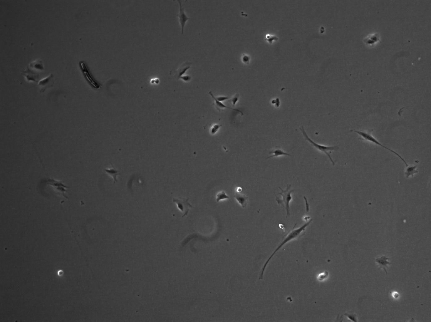
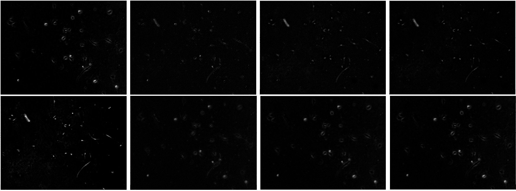
Figure 2: An input phase contrast image(Leftmost); Eight filtered outputs by applying filters on the image after the background subtraction(upper row are ${\Phi_{1},\cdots,\Phi_{4}}$; bottom row are ${\Phi_{5},\cdots,\Phi_{8}}$.)

2.1.1 Optimization

We now illustrate how to optimize Eq. 3 based on the Augmented Lagrange Multipliers (ALM) [7, 12]. We introduce the Lagrange multiplier ${\large\bf Y}$, the problem can be rewritten as

$$L({\large\bf B,E},\lambda)=\lVert{\large\bf B}\rVert_{\ast}+\lambda\lVert{\large\bf E}\rVert_{gfl}+\langle{\large\bf Y,A-B-E}\rangle$$ (4)

$$+\frac{\mu}{2}\lVert{\large\bf A-B-E}\rVert^{2}_{F},$$

where $\mu$ is a positive scalar. The optimal solution of ${\large\bf B}$ and ${\large\bf B}$ can be computed in an alternative way. Firstly, we update the ${\bf B_{t+1}}$ by fixing ${\bf E}={\bf E}_{t}$,

$${\large\bf B}_{t+1}=\arg\min_{{\large\bf B}}L({\large\bf B},{\large\bf E}_{t},{\large\bf Y}_{t},\mu_{t})$$ (5)

$$=\arg\min_{{\large\bf B}}\lVert{\large\bf B}\rVert_{\ast}+\langle{{\large\bf Y}_{t},{\large\bf A}-{\large\bf B}-{\large\bf E}_{t}}\rangle$$

$$+\frac{\mu_{t}}{2}\lVert{\large\bf A-B}-{\large\bf E}_{t}\rVert^{2}_{F},$$

Next, we update E by fixed the ${\bf B}$ as:

$${\large\bf E}_{t+1}=\arg\min_{\large\bf E}L({\large\bf B}_{t+1},{\large\bf E},{\large\bf Y}_{t},\mu_{t})$$ (6)

$$=\arg\min_{\large\bf E}\lambda\lVert{\large\bf E}\rVert_{gfl}+\langle{\large\bf Y}_{t},{\large\bf A}-{\large\bf B}_{t+1}-{\large\bf E}\rangle$$

$$+\frac{\mu_{t}}{2}\lVert{\large\bf A}-{\large\bf B}_{t+1}-{\large\bf E}\rVert^{2}_{F},$$

In each iteration, the Lagrange multiplier is updated as:

$${\large\bf Y}_{t+1}={\large\bf Y}_{t}+\mu_{t}({\large\bf A}-{\large\bf B}_{t+1}-{\large\bf E}_{t+1}),$$ (7)

Meanwhile, the parameter $\mu_{t}$ is updated accordingly as:

$$\mu_{t+1}=\begin{cases}{\rho\mu_{t}},\textup{if}\ \mu_{t}\lVert{\large\bf E}_{t+1}^{\ast}-{\large\bf E}_{t}^{\ast}\rVert_{F}/{\lVert{\large\bf A}\rVert}_{F}<\varepsilon\\ \mu_{t},\ \textup{otherwise}\end{cases}$$ (8)

where $\rho$ is a constant that is larger than $1$; $\varepsilon$ is a very small positive scalar.

2.2 Inverse Diffraction Pattern(IDP) filtering

In [8], the phase contrast microscopy image is approximated by a linear combination of $M$ diffraction patterns as:

$$\!g\!\propto\!\sum_{m=1}^{M}\!\Phi_{m}\!\ast\![sin\theta_{m}\delta(r)\!+\!(\varsigma_{p}cos\theta_{m}\!-\!sin\theta_{m})airy(r)],$$ (9)

where ${\theta_{m}}$ denotes the $\emph{m-}th$ phase retardation, which is defined as $\theta_{m}=2\pi\frac{m-1}{M}$; $\delta(r)$ is the Dirac delta function; $\varsigma_{p}$ is the amplitude attenuation factor caused by the phase ring, and we treat it as a constant at here; $\Phi_{m}$ is the coefficient of $\emph{m-}th$ basis; $airy(r)$ is an obscured airy pattern with the radius $r$ that is defined in [8]. For simplification, we define that

$$PSF(\theta_{m})=sin\theta_{m}\delta(r)\!+\!(\varsigma_{p}cos\theta_{m}\!-\!sin\theta_{m})airy(r),$$ (10)

where $PSF(\theta_{m})$ is the point spread function of the phase retardation $\theta_{m}$.

Mathematically, this is convolution process that images convolve with a complicated kernel. In order to restore the ideal image, we need deconvolution process that reverses the effects of the convolution on the observed data. More specifically, we need to seek the solution of a convolution equation of the form:

$$h\ast f=y,$$ (11)

where h is the ideal image and contaminated by convolving with the kernel f. The convolution result, which is the observed image, is y. To serve such purpose, we apply deconvolution in the Frequency domain, which is written as:

$$HF=Y,$$ (12)

where Y, H and F denote the Fourier transformation of y, h and f respectively. By computing the inverse filter of F as

$${F^{-1}}=\frac{H}{Y},$$ (13)

we can restore the ${H}$ as ${F^{-1}FH=H}$. Consequently, the inverse filter can be computed in the time domain as

$${f^{-1}}=\mathfrak{F}^{-1}(F^{-1}),$$ (14)

where ${f^{-1}}$ is the inverse filter of $f$; $\mathfrak{F}^{-1}$ is the inverse Fourier transform. With the definition of $PSF^{-1}(\theta_{m})$ as the inverse of the $PSF(\theta_{m})$, which is called as inverse diffraction pattern (IDP) and shown in Figure 2, we can recover ideal images as:

$$\Phi_{m}=\bar{g}\ast PSF^{-1}(\theta_{m}),$$ (15)

where $\bar{g}$ is the phase contrast microscopy image after background subtraction by the proposed method.

Usually, simple deconvolution is not robust due to the influence of noise, especially artifacts. In the presence of non-negligible noise, noise amplification will cause severe distortion [4]. The reason makes it success in our task is that noise is suppressed successfully by the proposed background subtraction method. Since the imaging condition is maintained to be unchanged for a certain sequence, the noise is also similar in each frame. Thus, the noise among frames are also approximately linearly correlated, which is similar to the medium. Thus, it can be treated as a part of the background and removed by the proposed method efficiently.

3 Experimental Results

	Dish1	Dish2	Dish3
Otsu threshold [5]	0.677	0.665	0.628
RPCA [10] + IDP	0.964	0.943	0.930
Cell-sensitive [13]	0.993	0.994	0.975
Ours	0.995	0.995	0.978

Table 1: The comparison of cell segmentation ACC on three dishes.

3.1 Evaluation Metrics and Data

	Dish1	Dish2	Dish3	Time
Preconditioning [11]	0.974	0.974	0.956	262 sec
Ours	0.995	0.995	0.981	$<$ 1 sec

Table 2: Performance comparison between ours and the Preconditioning restoration method.

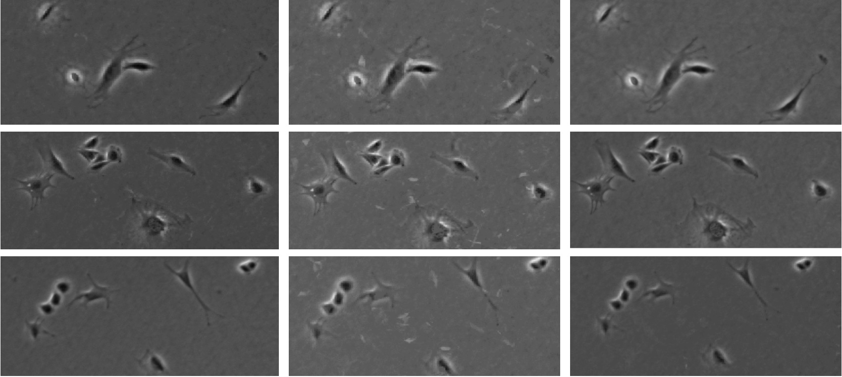
Figure 3: Left: input images; Middle: the background subtraction results by RPCA; Right: the background subtraction results by ours

The evaluation metric and data in [13] are adopted in the experiments to facilitate comparisons with related works. The definition of the evaluation metric, accuracy, is $ACC=(\lvert TP\rvert+\lvert N\rvert-\lvert FP\rvert)/(\lvert P\rvert+|N\rvert)$, where $P$ denotes the positives, $N$ denotes the negatives, $TP$ denotes the true positives and $FP$ denotes the false positives. The data set consists of three different cell dishes under different exposure durations and the ground truth data is labeled by two annotators.

3.2 Comparison and Evaluation

We conduct the performance comparison with different methods, shown in Table 1. Both the preconditioning method [11] and the proposed method achieved satisfactory results, where ours is slightly better than the preconditioning method. Our speed is much faster than the preconditioning method on these datasets, shown in Table 2. Although the performance of the proposed method is comparable to the cell-sensitive imaging [13], the proposed method holds some advantages. In cell-sensitive imaging method, the exposure time of images is a required parameter. Since the imaging information is not always available, this limits its application. Our method is designed to be independent of such parameters. This makes the proposed method more generally applicable. Also, our results demonstrate that the proposed method has better performance on removing artifacts in background images when compared to the cell-sensitive imaging method, shown in Figure 4. For qualitative evaluation, Figure 5 shows more results on background subtraction and restored artifact-free phase contrast images by the proposed method.

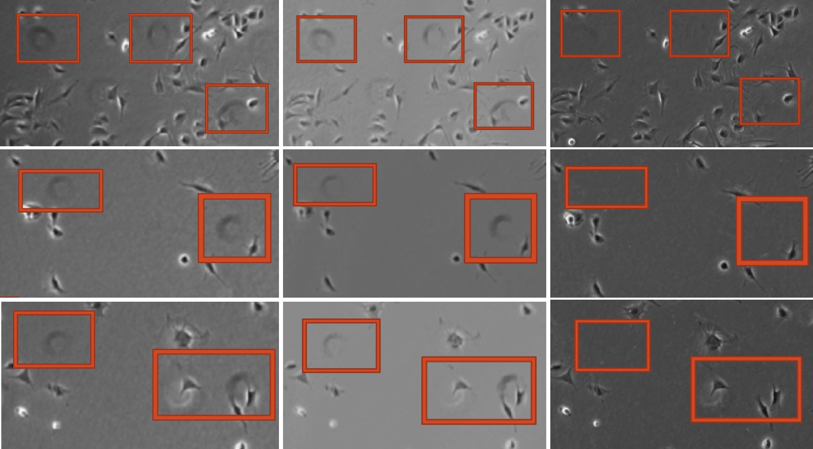
Figure 4: Left: input images with artifacts(red box); Middle: the results by cell-sensitive imaging method; Right: the results by the proposed background subtraction method

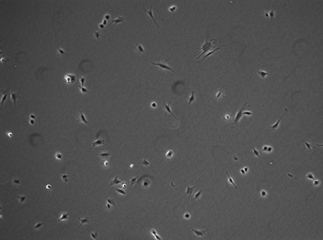
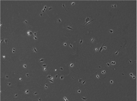
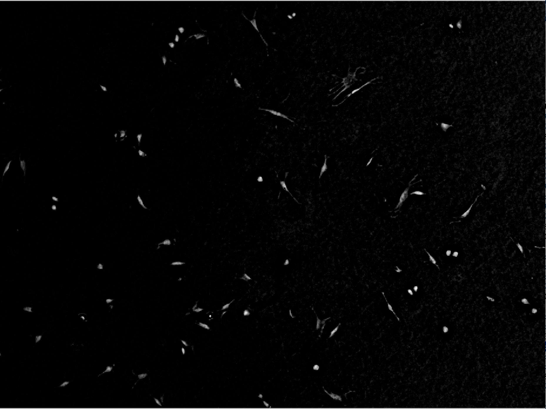
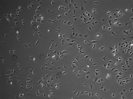
Figure 5: Column 1: input phase contrast images; Column 2: images after background subtraction; Column 3: restored phase contrast images by deconvolution;

4 Conclusion

In this paper, we propose a new approach for cell segmentation with two stages. We first remove background through a low-rank and sparse matrix decomposition. Then we obtain the accurate cells by introducing the inverse diffraction pattern filtering. It is inspired by optics model based restoration methods but much more efficient than them. Our experiments validate the effectiveness of the proposed method on cell segmentation.

References

- [1] J. Funke, F. A. Hamprecht, and C. Zhang. Learning to segment: Training hierarchical segmentation under a topological loss. In N. Navab, J. Hornegger, W. M. W. III, and A. F. Frangi, editors, MICCAI (3), volume 9351 of Lecture Notes in Computer Science, pages 268–275. Springer, 2015.
- [2] K. Li, M. Chen, and T. Kanade. Medical Image Computing and Computer-Assisted Intervention – MICCAI 2007: 10th International Conference, Brisbane, Australia, October 29 - November 2, 2007, Proceedings, Part II, chapter Cell Population Tracking and Lineage Construction with Spatiotemporal Context, pages 295–302. Springer Berlin Heidelberg, Berlin, Heidelberg, 2007.
- [3] D. T. Michael Kass, Andrew Witkin. Snakes: active contour models. International Journal of Computer Vision, 1:pp 321–331, 1988.
- [4] A. M.R.Banhamand. Digital image restoration. Signal Processing Magazine, IEEE, 1:14(2):24–41., 1997.
- [5] N. Otsu. A threshold selection method from gray-level histograms. IEEE Trans. Syst., Man, Cybernet, page 62–66, 1979.
- [6] J. Pan, T. Kanade, and M. Chen. Heterogeneous conditional random field: Realizing joint detection and segmentation of cell regions in microscopic images. In Computer Vision and Pattern Recognition (CVPR), 2010 IEEE Conference on, pages 2940–2947, June 2010.
- [7] Y. Peng, A. Ganesh, J. Wright, W. Xu, and Y. Ma. Rasl: Robust alignment by sparse and low-rank decomposition for linearly correlated images. pages 763–770, June 2010.
- [8] H. Su, Z. Yin, T. Kanade, and S. Huh. Phase contrast image restoration via dictionary representation of diffraction patterns. pages 615–622, 2012.
- [9] J. Wright, A. Ganesh, S. Rao, Y. Peng, and Y. Ma. Robust principal component analysis: Exact recovery of corrupted low-rank matrices via convex optimization. pages 2080–2088, 2009.
- [10] B. Xin, Y. Tian, Y. Wang, and W. Gao. Background subtraction via generalized fused lasso foreground modeling. CoRR, abs/1504.03707, 2015.
- [11] Z. Yin, T. Kanade, and M. Chen. Understanding the phase contrast optics to restore artifact-free microscopy images for segmentation. Medical Image Analysis, 16(5):1047–1062, 2012.
- [12] M. C. Z. Lin and Y. Ma. The augmented lagrange multiplier method for exact recovery of corrupted low-rank matrices. arXiv preprint arXiv:1009.5055,, 2010.
- [13] E. K. M. L. Zhaozheng Yin, Hang Su and H. Li. Cell sensitive phase contrast microscopy imaging by multiple exposures. Medical Image Analysis (MedIA), 2015.