Lattice QCD calculations of the quark and gluon contributions to the proton spin

Abstract:

A review of the calculations of the proton’s spin using lattice QCD is presented. Results for the three contributions, the quark contribution $\sum_{q=u,d,s,c}(\frac{1}{2}{\Delta q})$, the total angular momentum of the quarks $J_{q}$ and of the gluons $J_{g}$, and the orbital angular momentum of the quarks are discussed. The best measured is the the quark contribution $\sum_{q=u,d,s,c}(\frac{1}{2}{\Delta q})$, and its analysis is used to discuss the relative merits of calculations by the PNDME, ETMC and $\chi$QCD collaborations and the level of control over systematic errors achieved in each. The result by the PNMDE collaboration, $\sum_{q=u,d,s}\left[\frac{1}{2}{\Delta q}\right]=0.143(31)(36)$, is consistent with the COMPASS analysis $0.13<\frac{1}{2}\Delta\Sigma<0.18$. Results for $J_{q}$ and $J_{g}$ by the ETMC collaborations are also consistent with phenomenology. Lastly, I review first results from the LHPC collaboration for the calculation of the orbital angular momentum of the quarks. With much larger computing resources anticipated over the next five years, high precision results for all three will become available and provide a detailed description of their relative contributions to the nucleon spin.

1 Introduction

The spin is a fundamental defining property of the proton along with its mass, charge and magnetic moment. The simplest quark model picture would indicate that $S=1/2$ arises as a vector sum of the spins of the three valence quarks. In 1987, the European Muon Collaboration presented the remarkable result that the sum of the spins of the quarks contributes less than half of the total spin of the proton based on measurements of the spin asymmetry in polarized deep inelastic scattering [1]. This unexpected result was termed the “proton spin crisis”. The recent result of the COMPASS analysis is that the intrisic quark contribution to the proton’s spin is only about 30%, $0.13<\frac{1}{2}\Delta\Sigma<0.18$ at 3 GeV² [2].

Theoretically, the spin of the proton can be obtained by measuring a set of matrix elements of operators composed of quarks and gluons within the ground state of the nucleon. In this review, I will work with the gauge invariant decomposition of the nucleon’s total spin proposed by Ji [3]

$$\frac{1}{2}=\sum_{q=u,d,s,c,\cdot}\left(\frac{1}{2}{\Delta q}+L_{q}\right)+J_{g}$$ (1)

where ${\Delta q}\equiv{\Delta\Sigma_{q}}\equiv\langle 1\rangle_{\Delta q^{+}}\equiv g_{A}^{q}$ is the contribution of the intrinsic spin of a quark with flavor $q$; $L_{q}$ is the orbital angular momentum of that quark; and $J_{g}$ is the total angular momentum of the gluons. Thus, to explain the spin of the proton starting from QCD, one needs to calculate the contributions of all three terms. Of the three, the best determined is the first term, $\frac{1}{2}\Delta\Sigma\equiv\sum_{q=u,d,s}\frac{1}{2}{\Delta q}$. Results for which are presented here and have also been reviewed in the recent FLAG 2019 report [4].

Lattice QCD can unravel the mystery of where the proton gets its spin by measuring, from first principles, the matrix elements of appropriate quark and gluon operators within the nucleon state.

As orientation, the connection of the lattice QCD calculation of correlation functions from which matrix elements are extracted to an introductory course in non-relativistic quantum mechanics is conceptually simple. Simulations of lattice QCD using the path integral representation of the quantum field theory, provide the full relativistic Fock space wavefunction of a state (mesons or baryons) within which matrix elements can calculated. An illustration of the 2- and 3-point functions with the source and sink separated by Euclidean time $\tau$ and with the insertion of a quark bilinear operator $\overline{q}\Gamma q$, with $\Gamma$ one of the sixteen Dirac matrices, is given in Fig. 1. The three points are the source and sink at which the nucleon is created and annihilated using a suitable interpolating operator, and the timeslice of insertion on a quark line (valence or sea) of the quark bilinear operator whose matrix element is desired. Evaluating such correlation functions on each configuration, represents a “path”. The full nonperturbative wavefunction, and the matrix element of an operator within it, is then built up by the sum over all the “paths”, with the contribution of a given configuration weighted by its action. Expectations values of these correlation functions are finally obtained as the ensemble average over gauge configurations. To summarize, the elaborate machinery of lattice QCD, summarized briefly in Sec. 2, provides the non-perturbative wavefunction of the nucleon state within which the matrix elements of various operators can be calculated as ensemble averages.

To get high precision estimates for such nucleon n-point functions, the phase space of the path integral has to adequately covered, i.e., the ensemble should consist of a sufficiently large number of decorrelated gauge configurations. Next, all the systematic uncertainties introduced by discretizing QCD on a 4-d lattice need to be understood and controlled. Finally, lattice results that can be compared with experiments or phenomenology are obtained by performing a chiral-continuum-finite-volume (CCFV) fit to the data obtained over a range of values of $a$, $M_{\pi}$ and $L$ and evaluating the result at the physical pion mass $M_{\pi}=135$ MeV, taking the continuum limit defined by the lattice spacing $a\to 0$ and extrapolating in lattice size $L\to\infty$. A priori, one does not know how large a given systematic uncertainty in a given quantity is. It is largely determined a posteriori from the CCFV fits to the data. To increase the reliability of the CCFV fits and to control the total error requires high statistics data. In this review, I will devote considerable attention to how well the statistical and various systematic errors have been controlled and estimated in the various calculations.

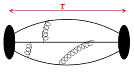
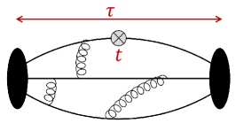
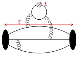
Figure 1: Illustration of the two- and three-point correlation functions calculated to extract the ground state nucleon matrix elements. (Left) the nucleon two-point function. (Middle) the connected three-point function with source-sink separation $\tau$ and operator insertion time slice $t$. (Right) the analogue disconnected three-point function that contributes to the flavor diagonal operators.

2 Flowchart of lattice QCD Calculation

The lattice methodology for the calculation of the contribution of the intrinsic spin of the quarks to the proton spin is mature. I will use it to exemplify, very briefly, the steps in the calculation.

• Formulate QCD on a finite 4-D Euclidean grid with lattice spacing $a$. This step defines the action ${\cal A}={\cal{A}}_{G}+\sum_{i}\overline{q}D_{i}q$ for the gauge and the quarks fields, and introduces discretization and finite volume errors. Here $D_{i}$ is the Dirac action for flavor $i$ and the sum is over the quark flavors. Since there is no one perfect lattice action that preserves all the properties of continuum QCD at finite $a$, a number of different actions have been used in simulations. They typically differ in how well the continuum chiral symmetry is preserved, the order $O(a^{n})$ of the discretization errors, and the cost of generation of ensembles of gauge configurations.

• In the path integral formulation of quantum field theory used in numerical simulations, the quark degrees of freedom are integrated out. The resulting Boltzmann weight, ${\cal{A}}={\cal{A}}_{G}+\sum_{i}{\rm Tr}\log D_{i}$, which is used to generate ensembles of background gauge fields, becomes a functional only of the gauge fields. The effects of quarks on the QCD vacuum are included through the term $\sum_{i}{\rm Tr}\log D_{i}$ in the Boltzmann weight used to generate lattices.

• A suite of ensembles of gauge configurations at multiple values of the lattice spacing and the light quark mass are generated with the chosen discretized action $\cal A$ using a Markov Chain Monte Carlo method with importance sampling. Simulations at a range of light quark masses at a fixed value of $a$ (equivalently the gauge coupling) are carried out to understand the chiral behavior of the observable and to improve the reliability of the extraction at the physical value taken to be $M_{\pi^{0}}=135$ MeV. With improvements in both algorithms and the computing power, current simulations include points at/near the physical pion mass. This has greatly improved the chiral fits and the extraction of results at the physical point $M_{\pi}=135$ MeV.

• Most calculations have, so far, been done assuming isospin symmetry, $m_{u}=m_{d}$, i.e., two degenerate light quark flavors. Thus effects proportional to $m_{d}-m_{u}$ are neglected. These are expected to be small for the quantities discussed here.

• Since the strange and charm quarks are relatively heavy, their contribution to the non-perturbative vacuum are included in the generation of gauge configurations with masses tuned to their physical values using appropriate spectral quantities, for example the masses of the $\Omega$ baryon and the $\eta_{c}$ meson. Thus, no fits in these quark masses are needed to get physical estimates. Simulations including these flavors are labeled 2+1 and 2+1+1 flavor calculations, respectively.

• The basic building blocks of the correlation functions are the gauge links and the quark propagators. Quark propagators, given by the inverse of the Dirac operator on a given configuration, are computed using Krylov solvers. Inverting the Dirac matrix, whether in gauge configuration generation or for quark propagators, is computationally the most expensive part of the calculation. The current algorithm of choice is the algebric Multigrid.

• Since the generation of gauge configurations is expensive, multiple measurements of correlation functions are made on each gauge configurations to increase the statistics. This exploits the fact that a large volume lattice can be considered to consist of many essentially decorrelated subvolumes.

• A large set of gauge invariant correlation functions (for example, for extracting matrix elements of different operators) are calculated at the same time by contracting the spin and color indices of quark propagators and gauge links in all possible combinations.

• Expectation values are constructed by averaging these correlation functions over measurements, i.e., over both multiple source points on a given configuration and over the ensemble of gauge configurations.

• Observables $O$, such as masses and matrix elements, are extracted from these expectation values using the spectral decomposition of the correlation functions. In this decomposition, the spectrum in a finite volume is defined by the eigenvalues of the transfer matrix.

• Different versions of an operator can be defined on the lattice and one can use any of these to calculate a given matrix elements. At finite $a$, results for different bare operators will, in general, differ. Renormalizing the operators removes the variation, and their matrix elements are finite in the continuum limit. In addition, to connect renormalized lattice results to those used by phenomenologists, the renormalization process includes a multiplicative matching factor from the lattice to some continuum scheme such as $\overline{MS}$ at a given scale, typically taken to be $\mu=2$ GeV.

• Lattice results obtained using renormalized operators depend on the lattice spacing, the pion mass (surrogate for the light quark mass), and the lattice size $L$. To obtain their physical value, $O_{\rm ph}$, lattice artifacts are removed by extrapolating $O(a,M_{\pi},L)$ to $a\to 0$, $M_{\pi}=135$ MeV and $L\to\infty$ using fits to data at multiple values of $a$, $M_{\pi}$ and $L$. These combined chiral-continuum-finite-volume (CCFV) fits are made using ansatz that are observable specific and physically motivated. For example, chiral perturbation theory is used to deduce the form of the correction terms with respect to $M_{\pi}$. The CCFV ansatz, with just the leader order correction terms, that is commonly used to fit the lattice data for the axial charges is

  $$g_{A}^{u,d,s}(a,M_{\pi},L)=g_{A}^{u,d,s}|_{\rm ph}+c_{2}a+c_{3}M_{\pi}^{2}+c_{4}M_{\pi}^{2}e^{-M_{\pi}L}\,,$$ (2)

  for lattice formulations in which discretization errors begin at $O(a)$ (PNDME). For the $\chi$QCD and ETMC calculations, this term should be read as $c_{2}a^{2}$.

2.1 Excited-State Contamination

An additional systematic error particularly relevant to the calculations of matrix elements within nucleon states is excited-state contamination. This is because interpolating operators used to create and annihilate nucleon states at either end the n-point correlation functions couple not just to the ground state nucleon but to all excitations and multiparticle states with the same quantum numbers. For baryons, the contribution of excited states is observed to be large because the number of states between 1.2–1.5 GeV grows with lattice volume. Their contributions need to be removed for each observable and on each ensemble before CCFV fits are made to get $O^{\rm ph}$. Two examples of excited-state contamination in the extraction of $g_{A}^{u-d}$ and its control by the PNDME Collaboration [5] using fits with up to three states in the spectral decomposition are shown in Fig. 2.

In the calculations reviewed, the excited state and the chiral-continuum fits were done separately for the connected and disconnected contributions. This is because the ranges of source-sink separation studied are typically different as are the number of ensembles analyzed. Such a separate analysis introduces an additional systematic that is judged to be small as explained in Ref. [6].

To obtain high-precision lattice results requires control over both statistical and the various systematic errors, i.e., excited-state contamination and those removed by the CCFV fits. In Section 3, I provide a critical analysis of the strengths and limitations of three calculations, PNDME [6], ETMC [7] and $\chi$QCD [8], of the quark contribution to the proton spin.

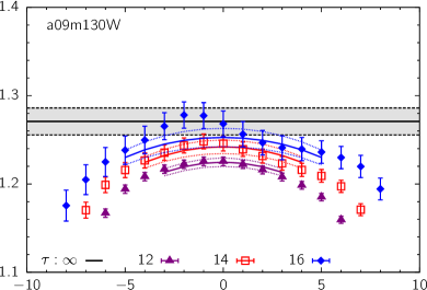
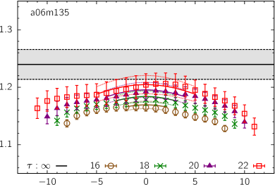
Figure 2: Illustration of the excited-state contamination in the extraction of $g_{A}^{u-d}$. Data from the two $M_{\pi}\approx 135$ MeV ensembles analyzed by the PNDME collaboration [5] are shown as a function of $t-\tau/2$ for various source-sink separations $\tau$. The grey band is the result for $g_{A}^{u-d}$ obtained in the $\tau\to\infty$ limit from a $3^{\ast}$-state fit. The colored lines show the fit for various values of $\tau$.

3 Intrinsic quark contribution to the proton spin

The intrinsic quark contribution to the proton spin is given by the flavor diagonal axial charges $g_{A}^{q}$. These are given by the matrix element of the flavor diagonal axial current, $\overline{q}\gamma_{\mu}\gamma_{5}q$,

$$g_{A}^{q}\overline{u}_{N}\gamma_{\mu}\gamma_{5}u_{N}\!=\!\langle N|Z_{A}\overline{q}\gamma_{\mu}\gamma_{5}q|N\rangle$$ (3)

where $Z_{A}$ is the renormalization constant and $u_{N}$ is the neutron spinor. In addition to quantifying the contribution of the quarks to the nucleon spin,

$$g_{A}^{q}\equiv\Delta q\!=\!\int_{0}^{1}dx(\Delta q(x)+\Delta\overline{q}(x))$$ (4)

is also the first Mellin moment of the polarized parton distribution function (PDF) integrated over the momentum fraction $x$ [9]. Thse are measured in semi-inclusive deep inelastic scattering experiments. The charges, $g_{A}^{u,d,s}$, also quantify the strength of the spin-dependent interaction of dark matter with nucleons [10, 11]. Of these, $\Delta s$ is the least well known and current phenomenological analyses [9] often rely on assumptions such as SU(3) symmetry and $\Delta s=\Delta\overline{s}$.

The most costly part of the calculation of $g_{A}^{u,d,s}$ is the contribution due to disconnected quark loops illustrated in Fig 1 (right). It is computed stochastically and then correlated with the nucleon two-point function. The resulting three-point function is then averaged over the ensemble of gauge configurations. The statistical error comes from both the stochastic evaluation (on each configuration) of the quark loop and it’s correlation with the nucleon 2-point function, and the ensemble average of the three-point function. Since the computational cost increases significantly as $M_{\pi}\to 135$ MeV, calculations of $g_{A}^{u,d,s}$ at the physical pion mass have started to be done only recently. The three results discussed in the next section include both disconnected contributions and evaluation of $g_{A}^{q}$ at $M_{\pi}=135$ MeV.

4 Lattice calculations of $g_{A}^{u,d,s}$

An overview of the lattice parameters of the results from three collaborations, PNDME [6], ETMC [7] and $\chi$QCD [8] that have presented results at the physical pion mass are given in Table 1. I will not review the work by JLQCD [12], LHPC [13] and Engelhardt [14] as they were done either at a single lattice spacing and/or with heavy quarks, and therefore cannot be compared to experimental/phenomenological results.

The results for connected and disconnected contributions for the three calculations reviewed are summarized in Table 2, and the final results in Table 3.

Collaboration	$N_{f}$	Formulation	$\#$ of	$a$	$M_{\pi}^{\rm val}$
			Ensembles	(fm)	(MeV)
PNDME [6]	2+1+1	Clover-on-HISQ	1	$0.15$	$321$
			4	$0.12$	$310,228$
			3	$0.087$	$313,226,138$
			3	$0.057$	$320,235,136$
$\chi$QCD [8]	2+1	Overlap-on-Domain Wall	1	$0.143$	147–327
		(Partially quenched)	1	$0.11$	254–389
			1	$0.083$	260–410
ETMC [7]	2	Twisted mass	1	0.094	130

Table 1: Lattice parameters of the three calculations discussed. The $\chi$QCD calculation consists of 5 or 6 values of the valence quark mass on each of the 3 ensembles constituting a partially quenched calculation.

Collaboration	$g_{A}^{u}|_{\rm Conn}$	$g_{A}^{d}|_{\rm Conn}$	$g_{A}^{u,d}|_{\rm disc}$	$g_{A}^{s}|_{\rm disc}$
PNDME [6]	0.895(21)	-0.320(12)	-0.118(14)	-0.053(8)
$\chi$QCD [8]	0.917(13(28)	-0.337(10)(10)	-0.070(12)(15)	-0.035(6)(7)
ETMC [7]	0.904(40)	-0.305(28)	-0.075(14)	-0.042(10)(2)

Table 2: Results for the flavor diagonal axial charges $g_{A}^{u,d,s}={\Delta q}$ for the proton. Results for the neutron can be obtained by interchanging the $u$ and $d$ flavor indices. All lattice results are quoted in $\overline{MS}$ scheme at 2 GeV².

Collaboration	$g_{A}^{u-d}$	$g_{A}^{u}$	$g_{A}^{d}$	$g_{A}^{s}$	$\sum_{q=u,d,s}(\frac{1}{2}{\Delta q})$
PNDME [6]	1.218(25)(30)	0.777(25)(30)	-0.438(18)(34)	-0.053(8)	0.143(31)(36)
$\chi$QCD [8]	1.254(16)(30)	0.847(18)(32)	-0.407(16)(18)	-0.035(6)(7)	0.203(13)(19)
ETMC [7]	1.212(40)	0.830(26)(4)	-0.386(16)(6)	-0.042(10)(2)	0.201(17)(5)

Table 3: Results for the flavor diagonal axial charges $g_{A}^{u,d,s}={\Delta q}$ for the proton. Results for the neutron can be obtained by interchanging the $u$ and $d$ flavor indices.

There are two obvious questions looking at the results in Tables 2 and 3: are the statistical and systematic errors in the three calculations equally well understood and controlled, and how much of the difference between the final results is due to the difference in the lattice parameters, listed in Table 1, that define the three calculations. Before answering the questions, I summarize the strengths and limitations of the three calculations to highlight the differences.

4.1 PNDME calculation

The connected parts of the PNDME 18A [6] results were obtained using eleven 2+1+1 flavour HISQ ensembles generated by the the MILC collaboration with $a\approx 0.057$, 0.87, 0.12 and 0.15 fm; $M_{\pi}\approx 135$, 220 and 320 MeV; and $3.3<M_{\pi}L<5.5$. The light disconnected contributions were obtained on six of these ensembles with the lowest pion mass $M_{\pi}\approx 220$ MeV, while the strange disconnected contributions were obtained on seven ensembles, i.e., including an additional one at $a\approx 0.087$ fm and $M_{\pi}\approx 135$ MeV. The CCFV fits to the connected contribution were done using the ansatz given in Eq. (2), and the finite volume correction was dropped for the analysis of the disconnected data.

The strengths of the PNDME calculation [6] with $2+1+1$ flavors of dynamical quarks are:

• High statistical precision with $O(10^{5})$ measurements performed on each ensemble.

• The data on the 11 ensembles cover a reasonable range in all three variables: $0.057<a<0.15$ fm, $135<M_{\pi}<320$ MeV and $3.3<M_{\pi}L<5.5$.

• The analysis of the excited-state contamination, discussed in Sec. 2, was done using three-state fits for the connected contribution and two-state fits for the disconnected contributions. Data at 4–5 values of the source sink separation $\tau$ in the range 1–1.5 fm were used in these fits.

• The CCFV fit was carried out keeping the leading terms in $a$, $M_{\pi}^{2}$ and $M_{\pi}L$ as defined in Eq. (2). Data from the two physical pion mass ensembles anchored the fit versus $M_{\pi}$. The Akaike Information Criteria [15] was used to justify not including higher order corrections, otherwise the fits would be over-parameterized.

• The CCFV fits are done separately for both the connected and disconnected contributions. The dominant variation in both was shown to be versus $a$.

The limitations of the PNDME calculation are:

• The mixed action, clover-on-HISQ, formulation is expected to give results for QCD in the $a\to 0$ limit. Ultimately, a confirmation using a unitary formulation is needed.

• The renormalization of the flavor diagonal charges is done assuming $Z_{A}^{\rm singlet}=Z_{A}^{\rm nonsinglet}$. While this has been validated to hold to within a percent by the ETMC and $\chi$QCD calculations, it needs to be confirmed for the clover-on-HISQ ensembles.

• Their estimate of the isovector axial charge $g_{A}^{u-d}=1.218(27)(30)$ is about 5% below the experimental value 1.277(2). The authors account for this deviation in the second systematic uncertainty of $0.030$ quoted in both $g_{A}^{u}$ and $g_{A}^{d}$.

4.2 $\chi$QCD calculation

The $\chi$QCD [8] calculation used three ensembles of $2+1$ flavors of dynamical domain-wall quarks generated by the RBC/UKQCD collaboration. Since two different discretizations of domain-wall fermions were used, the discretization effects in the CCFV fits require two separate $O(a^{2})$ terms. The strengths of the $\chi$QCD [8] calculation are:

• Both the sea and valence quark actions in the overlap-on-domain-wall formalism preserve the continuum chiral symmetry at finite $a$.

• The excited-state contamination is controlled using 2 states in the spectral decomposition of the 3-point data obtained at 4–5 values of the source sink separation $\tau$.

• Both renormalization factors, $Z_{A}^{\rm singlet}$ and $Z_{A}^{\rm nonsinglet}$, were calculated. They were found to agree to within a percent.

• The estimate of $g_{A}^{u-d}=1.254(16)(30)$ is consistent with the experimental value.

The limitations of the $\chi$QCD calculation are:

• The overlap-on-domain-wall formulation is also non-unitary.

• Only three approximate “unitary” points with lattice spacings 0.143, 0.11 and 0.083 fm and pion masses $M_{\pi}=171$, 337 and 302 MeV for the sea quarks, respectively, were analyzed. At each $a$, partially quenched data at 4–5 addition pion masses was collected. All the points (unitary and partially quenched) were analyzed together. In the chiral fit to this partially quenched data, possible dependence on $M_{\pi}^{\rm sea}$ was neglected and the data were fit versus only $M_{\pi}^{\rm valence}$.

• The CCFV fit used two terms of the form $c_{3}M_{\pi}^{2,{\rm sea}}+c_{3}^{v}M_{\pi}^{2,{\rm valence}}$ in Eq. (2), however, in practice, it was only sensitive to $M_{\pi}^{\rm valence}$. In the end, with only 3 “unitary” data points, Baysian priors were used to stabilize the two coefficients of the $O(a^{2})$ terms and the dependence on $M_{\pi}^{\rm sea}$ (sensitive only to the three approximately unitary points) and finite lattice size was neglected.

4.3 ETMC calculation

The strengths of the ETMC [7] calculation with $2$ flavors of dynamical quarks are:

• This is a unitary calculation. The same action, twisted mass with a clover term, is used for both the sea and valence quarks.

• The discretization errors in the twisted mass with a clover term formalism start at $O(a^{2})$.

• No extrapolation in $M_{\pi}$ was needed.

• Both renormalization factors, $Z_{A}^{\rm singlet}$ and $Z_{A}^{\rm nonsinglet}$, were calculated and found to agree to within a percent.

Limitations of the ETMC calculation are:

• The calculation used a single ensemble with $M_{\pi}=130$ MeV, $a=0.094$ and a relatively small $M_{\pi}L=2.98$. Thus discretization errors and finite lattice size corrections cannot be assessed.

• The estimate of $g_{A}^{u-d}=1.212(40)$ is about 5% below the experimental value 1.277(2).

4.4 My overall assessment of $g_{A}^{u,d,s}\equiv{\Delta\Sigma_{q}}$

Given that the three calculations differ in almost all aspects, it would seem unlikely that a simple explanation for the difference in the results shown in Table 3 can be presented. It turns out that the observed difference can be explained by the $a$ dependence found in the PNDME CCFV fits for the disconnected contributions shown in Fig. 3 if one assumes that there is no significant dependence on $N_{f}$, the lattice actions and the lattice size, and the excited-state fits and the chiral extrapolation are equally reliable.

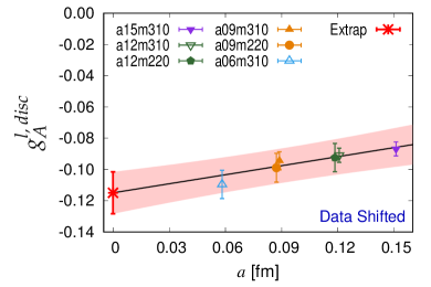
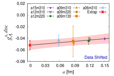
Figure 3: The chiral-continuum extrapolation of the renormalized $g_{A}^{l,{\rm disc}}$ and $g_{A}^{s,{\rm disc}}$ data using the ansatz given in Eq. (2). The pink band shows the result of the simultaneous fit plotted versus $a$. The data points have been shifted by extrapolating them to the physical point $M_{\pi}=135$ MeV using the fit.

Fig. 3 shows that the change between $a\approx 0.09$ fm and $a=0$ was found to be $\approx-0.04$ for $g_{A}^{l,{\rm disc}}$ and $\approx-0.01$ for $g_{A}^{s,{\rm disc}}$. Assuming that the same pattern of discretization corrections is applicable to the $\chi$QCD and ETMC results, then their values for $g_{A}^{u}$ would be smaller by $0.04$, those for $g_{A}^{d}$ more negative by $0.04$, and those for $g_{A}^{s}$ more negative by $0.01$. With these corrections, the results for the individual $g_{A}^{u,d,s}$ and for the sum $\frac{1}{2}{\Delta\Sigma}$ from the three calculations would overlap. Future higher precision data from more ensembles is, of course, necessary to validate this simple explanation.

5 Total angular momentum of quarks and gluons

The total angular momentum operator can be written in terms of the energy momentum tensor in a gauge invariant way as [3]

$$J^{i}=\frac{\epsilon^{ijk}}{2}\int d^{3}x(T^{0j}x^{k}-T^{0k}x^{j})$$ (5)

This can be further decomposed in terms of the contribution of quarks,

$$\vec{J}_{q}=\int d^{3}x\overline{q}\left[\vec{\gamma}\gamma_{5}+\vec{x}\times(-i\vec{D})\right]q,$$ (6)

and gluons

$$\vec{J}_{g}=\int d^{3}x(\vec{x}\times(\vec{E}\times\vec{B})\,.$$ (7)

To calculate these two contributions on the lattice, one evaluates the matrix elements of the following two operators within nucleon states:

$${O}_{q}^{\mu\nu}=\frac{1}{2}\left[\overline{q}\gamma^{(\mu}\stackrel{{\scriptstyle\rightarrow}}{{D}}{}^{\nu)}q+\overline{q}\gamma^{(\mu}\stackrel{{\scriptstyle\leftarrow}}{{D}}{}^{\nu)}q\right]\,,$$ (8)

and

$${O}_{g}^{\mu\nu}=\frac{1}{4}g^{\mu\nu}G^{2}-G^{\mu\alpha}G^{\nu}_{\alpha}\,.$$ (9)

The matrix elements of these operators at momentum transfer $Q^{2}\equiv(p^{\prime}-p)^{2}$ are then decomposed in terms of Lorentz covariant form factors as

$$\langle N(p^{\prime},s^{\prime})|{O}_{q,g}^{\mu\nu}|N(p,s)\rangle=\overline{u}_{N}(p^{\prime},s^{\prime})\Lambda_{q,g}^{\mu\nu}u_{N}(p,s)$$ (10)

where $P\equiv(p^{\prime}+p)/2$, $u_{N}$ is the nucleon spinor and

$$\Lambda_{q,g}^{\mu\nu}=A_{q,g}(Q^{2})\gamma^{\{\mu}P{}^{\nu\}}+B_{q,g}(Q^{2})\frac{P^{\{\mu}\sigma{}^{\nu\}\alpha}Q_{\alpha}}{2M_{N}}+C_{q,g}(Q^{2})\frac{Q^{\{\mu}Q^{\nu\}}}{M_{N}}$$ (11)

Here, $M_{N}$ is the nucleon mass and the curly braces denote that the two indices within them have to be symmetrized and the traceless part taken. From these, the total angular momentum is obtained from the following combination of the form factors

$$\vec{J}_{q,g}=\left[A_{q,g}(0)+B_{q,g}(0)\right]\,.$$ (12)

On the lattice, $A_{q,g}(0)$ can be extracted directly while $B_{q,g}(0)$ is obtained by extrapolating data at $Q^{2}\neq 0$ to $Q^{2}=0$.

The flowchart for the calculation of the three- point function from which $\langle N(p^{\prime},s^{\prime})|{O}_{q,g}^{\mu\nu}|N(p,s)\rangle$ are extracted is similar to that described in Sec. 2. There are, however, a number of additional challenges:

• ${O}_{q}^{\mu\nu}$ involves 1-link (one derivative) operators, and both connected and disconnected contributions need to be calculated.

• ${O}_{g}^{\mu\nu}$ is constructed out of Wilson loops. There is only a disconnected contribution with a noisier statistical signal.

• The matrix elements have to be decomposed in terms of form factors. The form factor $B_{q,g}(0)$ can only be evaluated at $Q^{2}\neq 0$ and the data extrapolated to $Q^{2}=0$.

5.1 ETMC Calculation of $J_{q}$ and $J_{g}$

As described above, the calculation of $J_{q}$ and $J_{g}$ is significantly harder and only the ETMC collaboration has presented results. Some details of the calculation are:

• The renormalization factor for ${O}_{q}^{\mu\nu}$ (involving one derivative operators) has been calculated non-perturbatively.

• The renormalization of ${O}_{g}^{\mu\nu}$ and its mixing with the quark singlet operator has only been carried out in 1-loop perturbation theory. The mixing is found to be a small correction.

• The stout smearing of gauge links in the operators brings the renormalization factor and mixing coefficient closer to their tree-level values [16].

• The disconnected contribution to $B_{q}(0)$ is found to be smaller than the statistical errors in the connected contributions. So $J_{s,c}\approx A_{s,c}(0)$ is used and $B_{q}(0)$ is neglected.

• The form factor $B_{g}(0)$ is assumed to be zero, so $J_{g}=A_{g}(0)$ is used.

• Checks on $A_{u-d}(0)$ are made by comparing with phenomenological values of the mean momentum fraction $\langle x\rangle_{u-d}=A_{u-d}(0)$.

Their results are

$$\vec{J}_{u+d+s}=0.255(12)(3)|_{\rm conn}+0.153(60)(47)|_{\rm disc}=0.408(61)(48)\,.$$ (13)

and

$$\vec{J}_{g}\approx A_{g}(0)=\frac{1}{2}\langle x\rangle_{g}=0.133(11)(14)\,.$$ (14)

Combining the two, the result for the spin of the nucleon is determined to be

$$J_{N}=\vec{J}_{q}+\vec{J}_{g}=0.541(62)(49)\,.$$ (15)

Within errors, the ETMC result is consistent with the proton spin being $1/2$.

6 Comparing results for quark angular momentum using Ji versus Jaffe-Manohar decompositions

Engelhardt [17, 18] has been developing methods to directly calculate the orbital angular momentum (OAM) of the quarks. The definition of OAM by Ji,

$$\vec{L}_{q}^{\rm Ji}=\int d^{3}x\ {q^{\dagger}}\left[\vec{x}\times i\vec{D}\right]q\,,$$ (16)

differs from that defined on the light-cone by Jaffe-Manohar [19],

$$\vec{L}_{q}^{\rm JM}=\int d^{3}x\ {q^{\dagger}}\left[\vec{x}\times i\vec{\nabla}\right]q\,,$$ (17)

in the form of the spatial derivative term. The relevant matrix elements required are of non-local quark bilinear operators connected by a staple shaped gauge connection shown in Fig. 4 (left). In this setup, the quark-antiquark is separated by distance $z$ in a direction that is transverse to both the average nucleon momentum $P$ and the momentum transfer $\Delta_{T}$; $p^{\prime}=P+\Delta_{T}$ and $p=P-\Delta_{T}$; and the nucleon spin and the staple direction $v$ are taken along the direction of $P$, which is typically taken to be the “3” direction. The matrix element of the operator with a straight link path ($\eta=0$) gives $\vec{L}_{q}^{\rm Ji}$, while the Jaffe-Manohar OAM, $\vec{L}_{q}^{\rm JM}$, is obtained in the limit $\eta\to\infty$. First results for both are presented in Ref. [18].

Results for the ratio $|\vec{L}_{q}^{\rm JM}|/|\vec{L}_{q}^{\rm Ji}|$ are shown in Fig. 4 (right). They indicate that $|\vec{L}_{q}^{\rm JM}|$ is about 40% larger than $|\vec{L}_{q}^{\rm Ji}|$. The difference is interpreted as the extra torque, due to final state interactions, accumulated by the struck quark as it flies out of the proton. Following up on this encouraging result, further work is in progress.

         

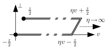
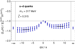
Figure 4: (Left) The geometry of the staple shaped gauge connection between the quark and antiquark used to study the Ji and Jaffe-Manohar orbital angular momentum of the quarks. (Right) The ratio $|\vec{L}_{q}^{\rm JM}|/|\vec{L}_{q}^{\rm Ji}|$ obtained on a 2+1-flavor clover ensemble with $M_{\pi}=317$ Mev and $a=0.114$ fm  [18].

7 Conclusions

This review makes the case that calculations of the nucleon spin from first principle simulations of lattice QCD are beginning to provide results with control over all systematics. Of the three contributions analyzed, the best determined is the quark contribution $\sum_{q=u,d,s,c}(\frac{1}{2}{\Delta q})$, followed by $J_{q}$ and finally $J_{g}$ and the orbital angular momentum of the quarks. The first results discussed are already consistent with phenomenology. The PNMDE collaboration have presented results for $\sum_{q=u,d,s}(\frac{1}{2}{\Delta q}$ with control over the various systematics. They find $\sum_{q=u,d,s}(\frac{1}{2}{\Delta q})=0.143(31)(36)$, consistent with the COMPASS value $0.13<\frac{1}{2}\Delta\Sigma<0.18$ obtained at 3 GeV² [2]. At the same time, the PNDME analysis makes a compelling case for the need for a new level of control over all systematic uncertainties in order to obtain results with $\leq 10\%$ total error.

The ETMC collaboration has presented first results for $J_{q}$ and $J_{g}$, and Engelhardt[18] for the orbital angular momentum of quarks. Over the next five years, with anticipated increase in computing resources, high precision results for all three will become available and provide an accurate picture of their relative contributions to the nucleon spin.

- [1] European Muon collaboration, J. Ashman et al., A Measurement of the Spin Asymmetry and Determination of the Structure Function g(1) in Deep Inelastic Muon-Proton Scattering, Phys. Lett. B206 (1988) 364.
- [2] COMPASS collaboration, C. Adolph et al., The spin structure function of the proton and a test of the Bjorken sum rule, Phys. Lett. B753 (2016) 18 [1503.08935].
- [3] X.-D. Ji, Gauge-Invariant Decomposition of Nucleon Spin, Phys. Rev. Lett. 78 (1997) 610 [hep-ph/9603249].
- [4] Flavour Lattice Averaging Group collaboration, S. Aoki et al., FLAG Review 2019, 1902.08191.
- [5] R. Gupta, Y.-C. Jang, B. Yoon, H.-W. Lin, V. Cirigliano and T. Bhattacharya, Isovector Charges of the Nucleon from 2+1+1-flavor Lattice QCD, Phys. Rev. D98 (2018) 034503 [1806.09006].
- [6] H.-W. Lin, R. Gupta, B. Yoon, Y.-C. Jang and T. Bhattacharya, Quark contribution to the proton spin from 2+1+1-flavor lattice QCD, Phys. Rev. D98 (2018) 094512 [1806.10604].
- [7] C. Alexandrou, M. Constantinou, K. Hadjiyiannakou, K. Jansen, C. Kallidonis, G. Koutsou et al., Nucleon Spin and Momentum Decomposition Using Lattice QCD Simulations, Phys. Rev. Lett. 119 (2017) 142002 [1706.02973].
- [8] J. Liang, Y.-B. Yang, T. Draper, M. Gong and K.-F. Liu, Quark spins and Anomalous Ward Identity, Phys. Rev. D98 (2018) 074505 [1806.08366].
- [9] H.-W. Lin et al., Parton distributions and lattice QCD calculations: a community white paper, Prog. Part. Nucl. Phys. 100 (2018) 107 [1711.07916].
- [10] A. L. Fitzpatrick, W. Haxton, E. Katz, N. Lubbers and Y. Xu, Model Independent Direct Detection Analyses, 1211.2818.
- [11] R. J. Hill and M. P. Solon, Standard Model anatomy of WIMP dark matter direct detection II: QCD analysis and hadronic matrix elements, Phys. Rev. D91 (2015) 043505 [1409.8290].
- [12] JLQCD collaboration, N. Yamanaka, S. Hashimoto, T. Kaneko and H. Ohki, Nucleon charges with dynamical overlap fermions, Phys. Rev. D98 (2018) 054516 [1805.10507].
- [13] J. Green, N. Hasan, S. Meinel, M. Engelhardt, S. Krieg, J. Laeuchli et al., Up, down, and strange nucleon axial form factors from lattice QCD, Phys. Rev. D95 (2017) 114502 [1703.06703].
- [14] M. Engelhardt, Strange quark contributions to nucleon mass and spin from lattice QCD, Phys. Rev. D86 (2012) 114510 [1210.0025].
- [15] H. Akaike, A new look at the statistical model identification, IEEE Transactions on Automatic Control 19 (1974) 716.
- [16] C. Alexandrou, M. Constantinou, K. Hadjiyiannakou, K. Jansen, H. Panagopoulos and C. Wiese, Gluon momentum fraction of the nucleon from lattice QCD, Phys. Rev. D96 (2017) 054503 [1611.06901].
- [17] M. Engelhardt, Quark orbital dynamics in the proton from Lattice QCD – from Ji to Jaffe-Manohar orbital angular momentum, Phys. Rev. D95 (2017) 094505 [1701.01536].
- [18] M. Engelhardt, J. Green, N. Hasan, S. Krieg, S. Meinel, J. Negele et al., Quark orbital angular momentum in the proton evaluated using a direct derivative method, PoS SPIN2018 (2019) 047 [1901.00843].
- [19] R. L. Jaffe and A. Manohar, The G(1) Problem: Fact and Fantasy on the Spin of the Proton, Nucl. Phys. B337 (1990) 509.