OGLE-2018-BLG-0022: First Prediction of an Astrometric Microlensing Signal from a Photometric Microlensing Event

Abstract

In this work, we present the analysis of the binary microlensing event OGLE-2018-BLG-0022 that is detected toward the Galactic bulge field. The dense and continuous coverage with the high-quality photometry data from ground-based observations combined with the space-based Spitzer observations of this long time-scale event enables us to uniquely determine the masses $M_{1}=0.40\pm 0.05~{}M_{\odot}$ and $M_{2}=0.13\pm 0.01~{}M_{\odot}$ of the individual lens components. Because the lens-source relative parallax and the vector lens-source relative proper motion are unambiguously determined, we can likewise unambiguously predict the astrometric offset between the light centroid of the magnified images (as observed by the Gaia satellite) and the true position of the source. This prediction can be tested when the individual-epoch Gaia astrometric measurements are released.

1. Introduction

Full characterization of a microlens requires the determination of its mass, $M$. For this determination, one has to measure both the angular Einstein radius, $\theta_{\rm E}$, and the microlens parallax, $\pi_{\rm E}$, i.e.,

$$M={\theta_{\rm E}\over\kappa\pi_{\rm E}},$$ (1)

where $\kappa=4G/(c^{2}~{}{\rm au})$. In order to determine $\theta_{\rm E}$, one has to detect deviations in the lensing light curve caused by finite source effects. For single-lens events, which comprise the overwhelming majority of lensing events, it is difficult to measure $\theta_{\rm E}$ because finite-source effects can be detected only for the very rare cases in which the lens passes over the surface of the source star. Determination of $\pi_{\rm E}$ requires to detect subtle deviations in the lensing light curve caused by the positional change of the source induced by the orbital motion of Earth around the Sun (Gould, 1992). However, such a parallax signal can be securely detected only for long time-scale events observed with a high-quality photometry. As a result, lens mass determinations by simultaneously measuring $\theta_{\rm E}$ and $\pi_{\rm E}$ have been confined to a very small fraction of all events.

In addition to photometric data, lens characteristics can be further constrained with astrometric data. By measuring the lensing-induced positional shifts of the image centroid using a high-precision instrument such as Gaia (Gaia Collaboration, 2016), the chance to measure the lens mass becomes higher (Paczyński, 1996). Astrometric microlensing observation is especially important to detect black holes (BHs), including isolated BHs, because the time scales are long for events produced by BHs and thus the probability to measure $\pi_{\rm E}$ is high. One can also measure the angular Einstein radius because astrometric lensing signals scale with $\theta_{\rm E}$.

To empirically verify the usefulness of Gaia lensing observations in characterizing microlenses, it is essential to predict Gaia astrometric signature on real microlensing events, and then confirm that the actual observations agree with these predictions. To do this, one needs a lensing event with not only a robust and unique solution but also relatively bright source. Unfortunately, such events are very rare because lensing solutions are, in many cases, subject to various types of degeneracy, e.g., the close/wide binary degeneracy (Griest & Safazadeh, 1998; Dominik, 1999; An, 2005), the ecliptic degeneracy (Smith et al., 2003; Skowron et al., 2011), the degeneracy between microlens-parallax and lens-orbital effects (Batista et al., 2011; Skowron et al., 2011; Han et al., 2016), the 4-fold degeneracy for space-based microlens parallax measurement (Refsdal, 1966; Gould, 1994; Zhu et al., 2015), etc.

In this work, we present the analysis of the binary-lens event OGLE-2018-BLG-0022. The dense and continuous coverage with high-quality photometric data from ground-based observations combined with space-based Spitzer observations of this long-timescale event yields a lensing solution without any degeneracy, leading to the unique determination of the physical lens parameters. Combined with the relative bright source, the event is an ideal case in which astrometric lensing signals can be predicted from the photometric data and confirmed from astrometric observations.

2. Observation and Data

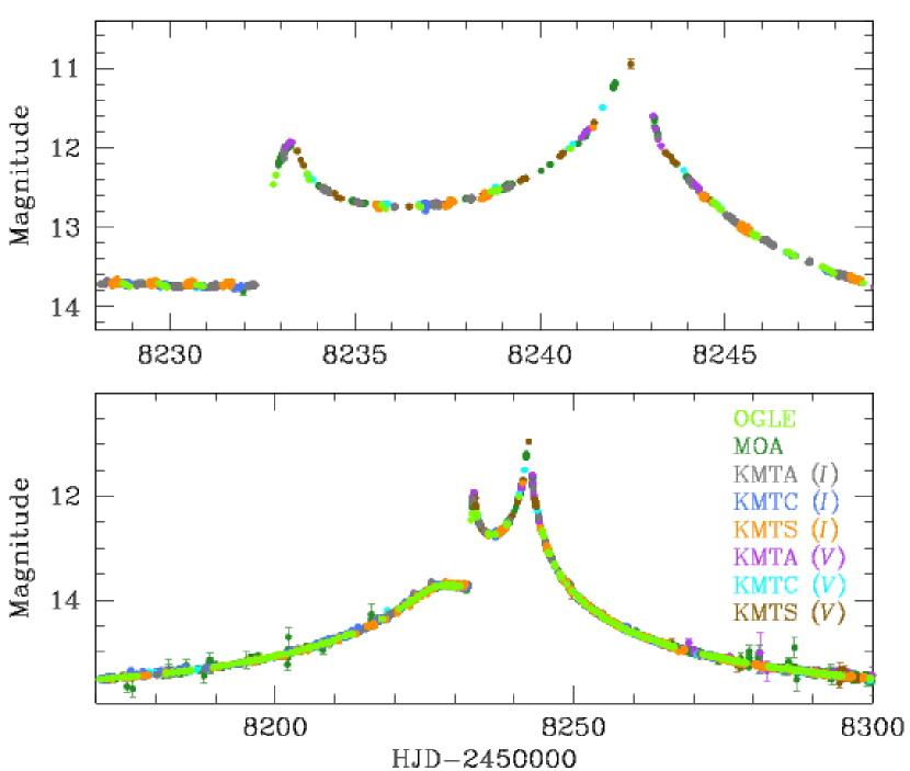
Figure 1.— Light curve of OGLE-2018-BLG-0022. The upper panels shows the zoom of the peak region. The colors of the data points match those of the labels of the telescopes used for observations.

The microlensing event OGLE-2018-BLG-0022 occurred on a star located toward the Galactic bulge field. The equatorial and galactic coordinates of the source are $({\rm RA},{\rm decl.})_{\rm J2000}=(17:59:27.04,-28:36:37.0)$ and $(l,b)=(1.82^{\circ},-2.44^{\circ})$, respectively. The source had a bright baseline magnitude of $I_{\rm base}=15.6$.

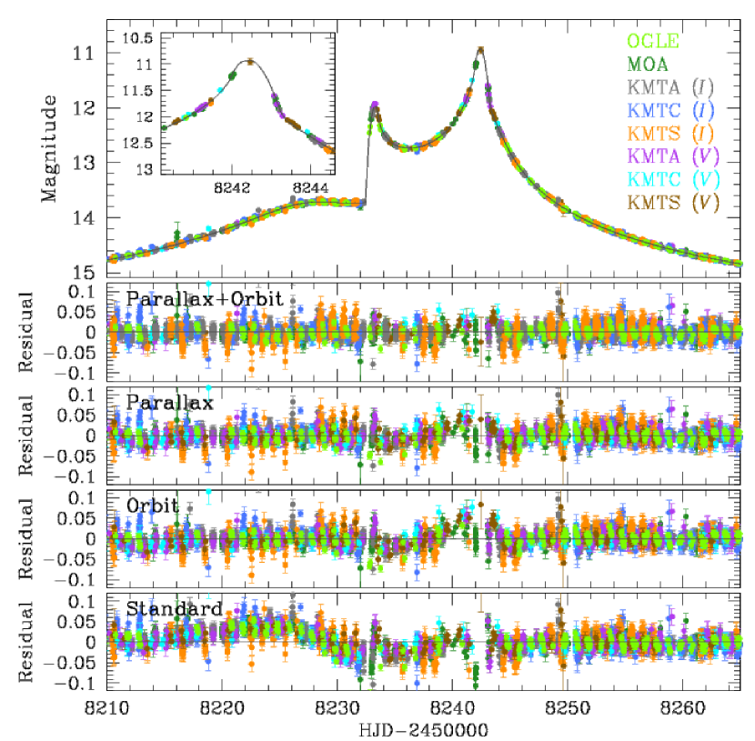
Figure 2.— Comparison of models obtained considering various higher-order effects. The top panel shows the data near the peak of the light curve, and the lower panels show the residuals from the tested models. The model curve superposed on the data points is the best-fit model considering both the microlens-parallax and lens-orbital effects.

Figure 1 shows the light curve of the event. It is characterized by two caustic-crossing spikes that occurred at ${\rm HJD}^{\prime}\equiv{\rm HJD}-2450000\sim 8233.0$ and $\sim 8242.5$ and a hump centered at ${\rm HJD}^{\prime}\sim 8227$. Caustics produced by a binary lens form close curves, and thus caustic crossings occur in multiples of two. Combined with the characteristic “U”-shape magnification pattern between the caustic spikes, the first and second spikes are inferred to be produced by the source’s caustic entrance and exit, respectively. The magnification pattern during the caustic entrance exhibits the typical shape when the source passes a regular fold caustic (Schneider & Weiss, 1986). However, the pattern during the second caustic spike appears to be different from a regular one, suggesting that another caustic feature is involved. The hump is likely to be produced by the source approach to a cusp of a caustic.

The event was discovered in the early 2018 bulge season by the OGLE survey (Udalski et al., 2015). The event is registered in the ‘OGLE-IV Early Warning System’ page as two identification (ID) numbers, OGLE-2018-BLG-0022 and OGLE-2018-BLG-0052. We use the former ID. The source was located also in the fields toward which two other lensing surveys of MOA (Bond et al., 2001) and KMTNet (Kim et al., 2016) were monitoring. In the list of ‘2018 MOA transient alerts’, the event was registered as MOA-2018-BLG-031. The lensing-induced brightening of the source started during the $\sim 3$-month time gap between the 2017 and 2018 bulge seasons. During this period, the Sun passed the bulge field and thus the event could not be observed. For this reason, at the first observation conducted in the 2018 bulge season on ${\rm HJD}^{\prime}=8151$ (February 1) the light curve was already $\sim 0.2$ mag brighter than the baseline magnitude. After being detected, the event lasted throughout the 2018 season. When the analysis of the event was completed, we learned that the event was additionally observed by the ROME/REA survey, which is a new survey commenced the 2018 season, and an independent analysis was in progress. We, therefore, conduct analysis based on the OGLE+MOA+KMTNet data sets.

We note that the event was very densely and continuously covered with an excellent photometric quality. The superb coverage was possible thanks to the high cadence of the survey observations conducted using globally distributed telescopes. The OGLE and MOA surveys utilize the 1.3 m telescope of the Las Campanas Observatory in Chile and the 1.8 m telescope located at Mt. John Observatory in New Zealand, respectively. The KMTNet survey uses 3 identical 1.6 m telescopes located at the Cerro Tololo Interamerican Observatory in Chile, the South African Astronomical Observatory, South Africa, and the Siding Spring Observatory, Australia. We designate the individual KMTNet telescopes as KMTC, KMTS, and KMTA, respectively. The OGLE survey observed the event with a cadence of $\sim 5$–6/night, and the KMTNet $I$-band and MOA cadences were 15 min and 10 min, respectively. In addition, KMTNet observed in $V$ band with a cadence of $\sim 2.5$ hours. The high photometric quality was achieved because the source star was very bright. The event brightness near the peak was brighter than $I\sim 12$, and many KMTNet data points near and above this limit were saturated. We exclude these data points. However, the KMTNet $V$-band points are not saturated, which is the reason for including them in the analysis. We note that there exist additional data obtained from space-based Spitzer observations. We will discuss the Spitzer data and the analysis of these data in Section 3.2.

The event was analyzed nearly in real time with the progress of the event. With the detection of the anomaly by the ARTEMiS system (Dominik et al., 2008), the first model was circulated to the microlensing community by V. Bozza. A. Cassan and Y. Hirao also circulated subsequent models. As the event proceeded, the models were further refined.

Reduction of the data was carried out using the photometry codes developed by the individual survey groups: Udalski (2003), Bond et al. (2001), and Albrow et al. (2009) for the OGLE, MOA, and KMTNet data sets, respectively. All of these codes are based on the difference imaging method (Alard & Lupton, 1998). For the KMTC $I$ and $V$-band data sets, additional photometry is conducted using the pyDIA code (Albrow, 2017) to measure the source color.

3. Analysis

3.1. Modeling Light Curve

Considering the characteristic caustic-crossing features, we conduct binary-lens modeling of the observed light curve. In the first-round modeling, we assume that the observer and the lens components do not experience any acceleration, and thus the relative lens-source motion is rectilinear. We refer to this model as the “standard” model.

Standard modeling requires seven lensing parameters, including the time of the closest lens-source approach, $t_{0}$, the separation at that time, $u_{0}$, the event timescale, $t_{\rm E}$, the projected separation, $s$, and the mass ratio between the lens components, $q$, the source trajectory angle, $\alpha$, and the normalized source radius, $\rho$. The lengths of $s$, $u_{0}$, and $\rho$ are normalized to $\theta_{\rm E}$. We compute finite-source magnifications considering the limb-darkening variation of the source star’s surface brightness. The profile of the surface-brightness is modeled by $S\propto 1-\Gamma_{\lambda}(1-1.5\cos\psi)$, where $\Gamma_{\lambda}$ denotes the linear limb-darkening coefficient and $\psi$ represents the angle between the normal to the source surface and the line of sight toward the source center. We adopt the limb-darkening coefficients from Claret (2000) considering the source type. The determination of the source type is discussed in section 3.3. The adopted limb-darkening coefficients are $\Gamma_{V}=0.726$, $\Gamma_{R}=0.639$, and $\Gamma_{I}=0.527$. We set the center of mass of the binary lens as the reference position. In the preliminary modeling, we conduct a grid search for $s$ and $q$ while the other parameters are searched for using a downhill approach based on the Markov chain Monte Carlo (MCMC) method. We then refine the solutions found from the preliminary search by allowing all parameters to vary.

Table 1Comparison of models

Model		$\chi^{2}$
Standard		21219.8
Orbit		14539.2
Parallax	($u_{0}>0$)	13765.0
–	($u_{0}<0$)	13764.5
Orbit + Parallax	($u_{0}>0$)	13029.7
–	($u_{0}<0$)	13256.0

The standard modeling yields a unique solution with binary lens parameters of $(s,q)\sim(0.51,0.35)$. This indicates that the lens is a binary composed of masses of a same order with a projected separation smaller than the angular Einstein radius, i.e., close binary ($s<1.0$). The event timescale is $t_{\rm E}\sim 67.6$ days, which is substantially longer than typical galactic lensing events. We check for the possible existence of a binary-lens solution with $s>1.0$, wide binary, caused by the close/wide binary degeneracy. We find that the fit of the best-fit wide-binary solution is worse than the fit of the close-binary solution by $\Delta\chi^{2}>20000$, indicating that the close/wide degeneracy is clearly resolved.

Although the standard model provides a fit that describes the overall light curve, we find that the model leaves systematic residuals. This can be seen in the bottom panel of Figure 2, which shows a relatively small ($\lesssim 0.05$ mag) but easily noticed deviation from the standard model in the region around the main anomaly features. We also find that the deviation persists throughout the light curve. This suggests the need to consider higher-order effects.

Noticing the residual from the standard model, we conduct additional modeling considering higher-order effects. It is known that two higher-order effects cause long-term deviations in lensing light curves. The first is the microlens-parallax effect, which is caused by the acceleration of the observer’s motion induced by the orbital motion of Earth around the Sun (Gould, 1992). The other is the lens-orbital effect, which is caused by the acceleration of the lens motion induced by the orbital motion of the lens (Dominik, 1998; Ioka et al., 1999). We test these effects by conducting three sets of additional modeling. In the “parallax” and “orbit” models, we separately consider the microlens-parallax and lens-orbital effects, respectively. In the “orbit+parallax” model, we simultaneously consider both effects. For events affected by the microlens-parallax effect, there usually exist a pair of degenerate solutions with $u_{0}>0$ and $u_{0}<0$. This so-called ‘ecliptic degeneracy’ is caused by the mirror symmetry of the source trajectory with respect to the binary axis (Smith et al., 2003; Skowron et al., 2011). We check this degeneracy when the microlens-parallax effect is considered in modeling.

Considering the higher-order effects requires one to include additional parameters in modeling. Parallax effects are described by 2 parameters of $\pi_{{\rm E},N}$ and $\pi_{{\rm E},E}$, which denote the two components of the microlens-parallax vector, $\mbox{\boldmath$\pi$}_{\rm E}$, projected onto the sky along the north and east directions in the equatorial coordinates, respectively. Under the approximation that the change of the lens position caused by the orbital motion is small, lens-orbital effects are described by 2 parameters of $ds/dt$ and $d\alpha/dt$, which represent the change rates of the binary separation and the orientation angle, respectively.

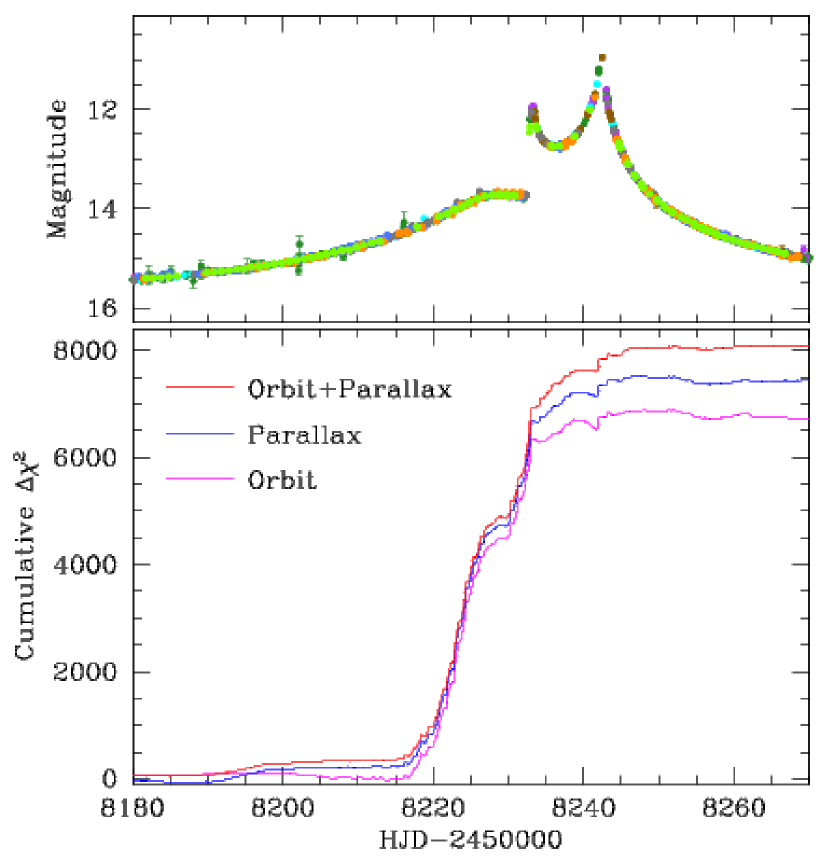
Figure 3.— Cumulative distribution of $\Delta\chi^{2}$ between the models with higher-order effects and the standard model.

In Table 1, we summarize the results of the additional modeling runs in terms of $\chi^{2}$ values. From the comparison of the model fits, we find the following results. First, the fit greatly improves with the consideration of the higher-order effects. We find that the fit improves by $\Delta\chi^{2}=6680.6$ and $7455.3$ with respect to the standard model by considering the lens-orbital and microlens-parallax effects, respectively, indicating that the higher-order effects are clearly detected. When both effects are simultaneously considered, the fit further improves by $\Delta\chi^{2}\sim 1509.5$ and 734.8 with respect to the orbit and parallax models, respectively. To visualize this improvement, we present the residuals of the tested models in the lower panels of Figure 2. In Figure 3, we also present the cumulative distributions of $\Delta\chi^{2}$ as a function of time to show the region of the fit improvement. It is found that the greatest fit improvement occurs in the region around the main features of the light curve, i.e., the hump and caustic spikes, although the fit improves throughout the event. Second, the ecliptic degeneracy between the solutions with $u_{0}>0$ and $u_{0}<0$ is also resolved. It is known that this degeneracy is usually very severe even for binary-lens events with well covered caustic features, e.g., $\Delta\chi^{2}\sim 3$ for OGLE-2017-BLG-053 (Jung et al., 2018) and $\Delta\chi^{2}\sim 8$ for OGLE-2017-BLG-0039 (Han et al., 2018b). For OGLE-2018-BLG-0022, we find that the solution with $u_{0}>0$ is preferred over the solution with $u_{0}<0$ by $\Delta\chi^{2}\sim 226.3$, which is big enough to clearly resolve the degeneracy.

Table 2Best-fit lensing parameters

parameter	Ground only	Ground+Spitzer
$t_{0}$ (${\rm HJD}^{\prime}$)	8238.467 $\pm$ 0.016	8238.490 $\pm$ 0.015
$u_{0}$	0.0085 $\pm$ 0.0001	0.0084 $\pm$ 0.0001
$t_{\rm E}$ (days)	71.19 $\pm$ 0.29	70.41 $\pm$ 0.25
$s$	0.528 $\pm$ 0.001	0.529 $\pm$ 0.001
$q$	0.302 $\pm$ 0.003	0.304 $\pm$ 0.003
$\alpha$ (rad)	0.176 $\pm$ 0.001	0.176 $\pm$ 0.001
$\rho$ ($10^{-3}$)	4.88 $\pm$ 0.05	4.97 $\pm$ 0.04
$\pi_{{\rm E},N}$	0.307 $\pm$ 0.020	0.242 $\pm$ 0.020
$\pi_{{\rm E},E}$	0.056 $\pm$ 0.001	0.052 $\pm$ 0.001
$ds/dt$ (yr-1)	0.511 $\pm$ 0.020	0.443 $\pm$ 0.020
$d\alpha/dt$ (yr-1)	0.506 $\pm$ 0.063	0.680 $\pm$ 0.061
$I_{s,{\rm OGLE}}$	15.86 $\pm$ 0.005	15.86 $\pm$ 0.005
$I_{b,{\rm OGLE}}$	18.85 $\pm$ 0.070	18.85 $\pm$ 0.070

Note. — ${\rm HJD}^{\prime}={\rm HJD-2450000}$. The values $I_{s,{\rm OGLE}}$ and $I_{b,{\rm OGLE}}$ represent the $I$-band magnitudes of the source and blend estimated based on the OGLE data, respectively.

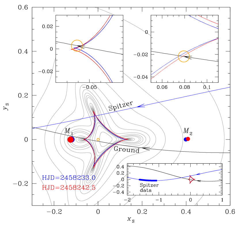
Figure 4.— Configuration of the lens system showing the source motion with respect to the caustic. The black and blue curves with arrows represent the source trajectories seen from the ground and the Spitzer telescope, respectively. The upper right and left insets show zoom of the regions around which the source entered and exited the caustic, respectively. The small orange circle on the source trajectory represents the source size. The grey curves around the caustic represent equi-magnification contours. Due to the change of the lens position caused by the orbital effect, we present the positions of the lens components ($M_{1}$ and $M_{2}$) and caustic at two epochs marked inside the main panel. The lower right inset shows a wider view to present the source positions when Spitzer observations were conducted (the region marked by thick line weight).

In the middle column of Table 2, we present the determined lensing parameters of the best-fit solution, i.e., orbit+parallax model with $u_{0}>0$. In Figure 4, we also present the lens-system configuration, which shows the source trajectory (the black curve with an arrow) with respect to the lens components (marked by $M_{1}$ and $M_{2}$) and caustic (closed curve composed of concave curves). It is found that the source passed almost parallel to the binary axis. The caustic, which is composed of 4 folds, is located between the lens components. The hump centered at ${\rm HJD}^{\prime}\sim 8227$ was produced when the source passed the excess magnification region extending from the right on-binary-axis caustic cusp. The source crossed the lower right fold caustic, producing the first caustic spike. Then, the source passed the upper left fold caustic, producing the second spike. To be mentioned is that the source enveloped the left on-axis caustic cusp during the caustic exit. See the left inset of Figure 4, which shows the enlargement of the caustic exit region. As a result, the caustic-crossing pattern differs from that produced when the source passes a regular fold caustic. See the inset in the upper panel of Figure 2.

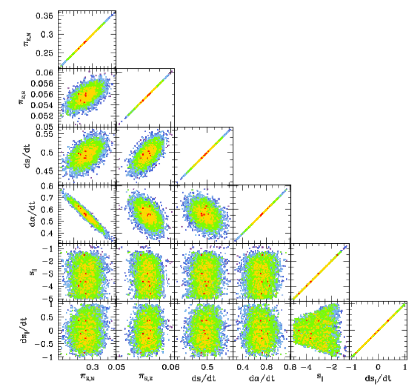
Figure 5.— $\Delta\chi^{2}$ distributions of MCMC points in the planes of the higher-order lensing-parameter combinations obtained from modeling considering full orbital parameters. The color coding indicates points within $1\sigma$ (red), $2\sigma$ (yellow), $3\sigma$ (green), $4\sigma$ (cyan), and $5\sigma$ (blue).

We note that OGLE-2018-BLG-0022 is a very rare case in which all the lensing parameters including those describing the higher-order effects are accurately determined without any ambiguity. As mentioned, the event does not suffer from the close/wide degeneracy, and thus there is no ambiguity in the binary separation. Furthermore, the ecliptic degeneracy is resolved with a significant confidence level, and thus the microlens parallax and the resulting lens mass are uniquely determined.

Prompted by the accuracy of modeling, we further check whether the determinations of the complete orbital parameters are possible for this event. This requires two additional parameters $s_{\parallel}$ and $ds_{\parallel}/dt$, which represent the line-of-sight binary separation normalized to $\theta_{\rm E}$ and the change rate of $s_{\parallel}$, respectively (Skowron et al., 2011; Shin et al., 2012). One also needs the information of the angular Einstein radius, and we describe the procedure for the $\theta_{\rm E}$ estimation in section 3.3. We find that it is difficult to determine the full orbital parameters. In Figure 5, we present the $\Delta\chi^{2}$ distributions of MCMC points in the planes of the higher-order lensing-parameter combinations. It is found that the additional two parameters ($s_{\parallel}$ and $ds_{\parallel}/dt$) are poorly constrained, while the other higher-order parameters ($\pi_{{\rm E},N}$, $\pi_{{\rm E},E}$, $ds/dt$, $d\alpha/dt$) are well constrained. We judge that the difficulty of full characterization of the orbital lens motion is caused by the short duration of the major anomaly features.

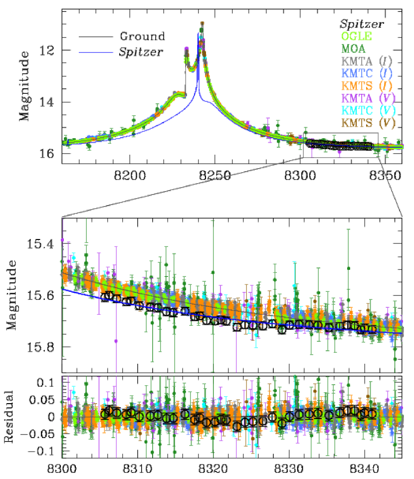
Figure 6.— Model light curves obtained from the combined analysis of the ground-based and space-based Spitzer data. The black and blue curves are for the ground-based and Spitzer data, respectively. The lower panels show the zoom of the region of the Spitzer data obtained during the period $8305.7\leq{\rm HJD}^{\prime}\leq 8341.0$.

3.2. Spitzer Data

In addition to the ground-based data, there exist data obtained from space-based Spitzer observations. Spitzer observations of the event were conducted in 3.6 $\mu$m channel ($L$ band) with 1-day cadence during the period $8305.7\leq{\rm HJD}^{\prime}\leq 8341.0$ and, in total, 34 data points were acquired. Data reduction was conducted using the procedure described in Calchi Novati et al. (2015). In Figure 6, we plot the Spitzer data over the data points from the ground-based observations.

Spitzer data may help to improve the accuracy of $\pi_{\rm E}$ measurement. This is because the Spitzer telescope is in a heliocentric orbit and thus the Earth-satellite separation and the physical Einstein radius, $r_{\rm E}=D_{\rm L}\theta_{\rm E}$, are of the same order of au. In this case, the light curve seen from space would be substantially different from the light curve observed from the ground (Refsdal, 1966; Gould, 1994), and thus space-based data can give an important constraint on the microlens parallax (Han et al., 2018a). We, therefore, check the effect of the Spitzer data on the $\pi_{\rm E}$ measurement. In the analysis with the additional Spitzer data, we impose a constraint of the source color with the measured instrumental value of $I-L=5.21\pm 0.02$ following the procedure described in Shin et al. (2017).

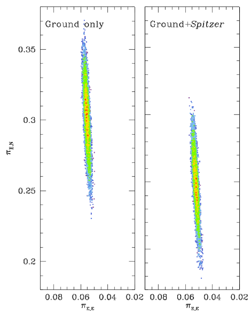
Figure 7.— $\Delta\chi^{2}$ distributions of MCMC points in the $\pi_{{\rm E},E}$–$\pi_{{\rm E},N}$ plane obtained from modelings with only ground-based data (left panel) and with additional space-based Spitzer data. The color coding indicates MCMC points within 1$\sigma$ (red), 2$\sigma$ (yellow), 3$\sigma$ (green), 4$\sigma$ (cyan), and 5$\sigma$ (blue) levels.

In the right column of Table 2, we present the lensing parameters estimated with the additional Spitzer data. From the comparison of the parameters with those estimated from the ground-based data, it is found that the parameters are similar to each other except for the slight differences in the higher-order parameters. In Figure 7, we present the $\Delta\chi^{2}$ distributions of MCMC points in the $\pi_{{\rm E},E}$–$\pi_{{\rm E},N}$ plane obtained from the modelings with (right panel) and without (left panel) the Spitzer data. It is found that the additional Spitzer data make the north component of the microlens parallax vector slightly smaller than the value estimated from the ground-based data.
In Figure 4, we present the source trajectory seen from the satellite (blue curve with an arrow marked by ‘Spitzer’). In Figure 6, we also present the model light curve for the Spitzer data (blue curve).

3.3. Angular Einstein Radius

We determine the angular Einstein radius, which is the other ingredient needed for the lens mass measurement besides $\pi_{\rm E}$, from the combination of the normalized source radius and the angular source radius, i.e., $\theta_{\rm E}=\theta_{*}/\rho$. The normalized source radius $\rho$ is determined by analyzing the caustic-crossing parts of the light curve. The angular source radius $\theta_{*}$ is estimated based on the de-reddened color, $(V-I)_{0}$, and brightness, $I_{0}$, of the source. We determine $(V-I)_{0}$ and $I_{0}$ using the method of Yoo et al. (2004), which utilizes the centroid of the red giant clump (RGC) in the color-magnitude diagram (CMD) as a reference.

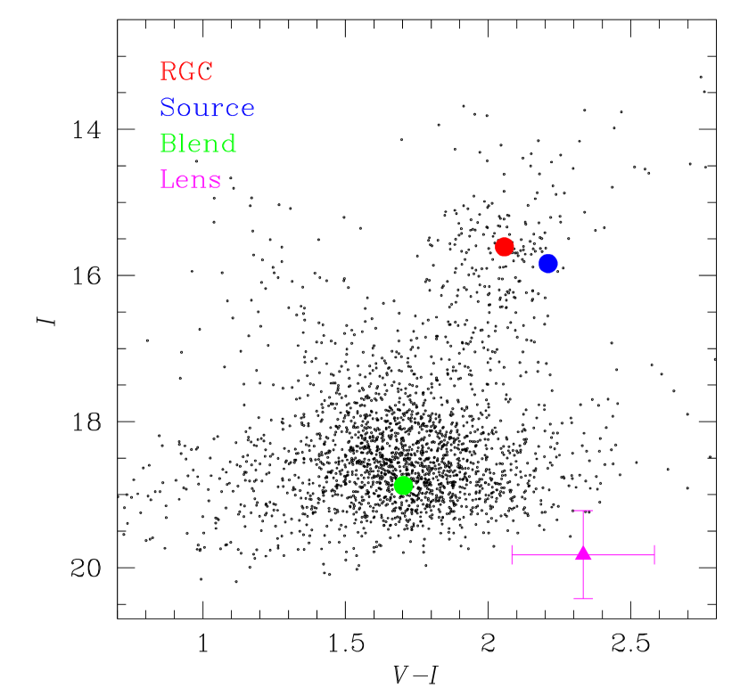
Figure 8.— Source position (blue dot) in the color-magnitude diagram of stars around the source. The red dot indicates the centroid of the red giant (RGC). The green dot represents the position of the blend, and the triangle dot with error bars denotes the expected position of the lens estimated from its mass and distance.

In Figure 8, we mark the position of the source with respect to the RGC centroid in the OGLE-III CMD. We note that the de-reddened source color and brightness are estimated using the $I$ and $V$-band pyDIA photometry of the KMTC data set. However, the magnitude of the KMTC data is not calibrated, while the OGLE-III data are calibrated (Szymański et al., 2011). We, therefore, place the source position on the calibrated OGLE-III CMD using the offsets in color and brightness between the RGC centroids of the KMTC and OGLE-III CMDs. With the apparent color and brightness of the source of $(V-I,I)=(2.21,15.86)$ and the RGC centroid of $(V-I,I)_{\rm RGC}=(2.06,15.61)$ combined with the known de-reddened values of the RGC centroid $(V-I,I)_{\rm RGC,0}=(1.06,14.35)$ (Bensby et al., 2011; Nataf et al., 2013), we estimate that the de-reddened color and brightness of the source are $(V-I,I)_{0}=(1.21,14.58)$, indicating that the source is a K-type giant. The measured $V-I$ color is converted into $V-K$ color using the color-color relation of Bessell & Brett (1988). We then estimate the angular source radius using the $(V-K)/\theta_{*}$ relation of Kervella et al. (2004). We estimate that the source has an angular radius of $\theta_{*}=6.54\pm 0.46~{}\mu{\rm as}$.

With the source radius, we estimate the angular Einstein radius of

$$\theta_{\rm E}=1.31\pm 0.09~{}{\rm mas}.$$ (2)

Combined with the measured event timescale $t_{\rm E}$, the relative lens-source proper motion as measured in the geocentric frame is estimated by

$$\mu_{\rm geo}={\theta_{\rm E}\over t_{\rm E}}=6.82\pm 0.48~{}{\rm mas}~{}{\rm yr}^{-1}.$$ (3)

In the heliocentric frame, the proper motion is

$$\mu_{\rm helio}=\left|\mu_{\rm geo}\,{\mbox{\boldmath$\pi$}_{\rm E}\over\pi_{\rm E}}+{\bf v}_{\oplus,\perp}{\pi_{\rm rel}\over{\rm au}}\right|=7.33\pm 0.52~{}{\rm mas}~{}{\rm yr}^{-1}.$$ (4)

Here ${\bf v}_{\oplus,\perp}(N,E)=(2.1,18.5)~{}{\rm km}~{}{\rm s}^{-1}$ denotes the projected velocity of Earth at $t_{0}$, $\pi_{\rm rel}={\rm au}(D_{\rm L}^{-1}-D_{\rm S}^{-1})$, and $D_{\rm S}$ denotes the distance to the source (Gould, 2004; Dong et al., 2009). In Table 3, we summarize the angular Einstein radius and the proper motion. Also listed is the angle of the heliocentric lens-source relative proper motion as measured from north toward east, i.e., $\phi_{\rm helio}=\tan^{-1}(\mu_{{\rm helio},E}/\mu_{{\rm helio},N})\sim 22^{\circ}$.

Table 3Einstein radius and proper motion

Quantity	Value
Angular Einstein radius	1.31 $\pm$ 0.09 mas
Proper motion (geocentric)	6.82 $\pm$ 0.48 mas yr-1
Proper motion (heliocentric)	7.32 $\pm$ 0.52 mas yr-1
$\phi_{\rm helio}$	$21.7^{\circ}\pm 1.5^{\circ}$

Note. — The angle $\phi_{\rm helio}$ represents the angle of the heliocentric lens-source relative proper motion as measured from north toward east.

Table 4Physical Lens Parameters

Quantity	Value
Mass of the primary lens	0.40 $\pm$ 0.05 $M_{\odot}$
Mass of the companion lens	0.15 $\pm$ 0.01 $M_{\odot}$
Distance to the lens	2.21 $\pm$ 0.18 kpc
Projected separation	1.54 $\pm$ 0.13 au
$({\rm KE}/{\rm PE})_{\perp}$	0.09 $\pm$ 0.01

Note. — $({\rm KE}/{\rm PE})_{\perp}$ represents the projected kinetic-to-potential energy ratio of the lens system.

3.4. Physical Lens Parameters

Being able to determine $\pi_{\rm E}$ and $\theta_{\rm E}$ without any ambiguity, the mass of the lens is uniquely determined. It is found that the lens is a binary composed of an early M-dwarf primary with a mass

$$M_{1}=0.50\pm 0.05~{}M_{\odot}$$ (5)

and a late M-dwarf companion with a mass

$$M_{2}=0.15\pm 0.01~{}M_{\odot}.$$ (6)

We note that the masses are estimated based on the solution obtained using both the ground-based and Spitzer data.

With the determined $\pi_{\rm E}$ and $\theta_{\rm E}$, the distance to the lens is determined by

$$D_{\rm L}={{\rm au}\over\pi_{\rm E}\theta_{\rm E}+\pi_{\rm S}}=2.21\pm 0.18~{}{\rm kpc},$$ (7)

indicating that the lens is in the disk. Here $\pi_{\rm S}={\rm au}/D_{\rm S}$. The source distance is estimated using the relation $D_{\rm S}=d_{\rm GC}/(\cos l+\sin l\cos\theta_{\rm bar}/\sin\theta_{\rm bar})\sim 7.87~{}{\rm kpc}$, where $d_{\rm GC}\sim 8160$ pc is the distance to the Galactic center and $\theta_{\rm bar}=40^{\circ}$ is the orientation angle of the bulge bar (Nataf et al., 2013). Once the distance is estimated, the projected separation between the lens components is estimated by

$$a_{\perp}=sD_{\rm L}\theta_{\rm E}=1.54\pm 0.13~{}{\rm au}.$$ (8)

For the source of the event, the parallax is not measured but the proper motion (in the heliocentric frame) is listed in the Gaia archive with values

$$\mbox{\boldmath$\mu$}_{\rm S}(N,E)=(-6.12,-2.76)~{}{\rm mas}~{}{\rm yr}^{-1}.$$ (9)

The proper motion indicates that the source is a typical bulge star. Since the relative lens-source proper motion (in the heliocentric frame), $\mu$, is related to the proper motions of the source, $\mbox{\boldmath$\mu$}_{\rm S}$, and the lens, $\mbox{\boldmath$\mu$}_{\rm L}$, by $\mbox{\boldmath$\mu$}=\mbox{\boldmath$\mu$}_{\rm L}-\mbox{\boldmath$\mu$}_{\rm S}$, the Gaia measurement of the source proper motion allows us to estimate the lens proper motion by the relation

$$\mbox{\boldmath$\mu$}_{\rm L}(N,E)=\mbox{\boldmath$\mu$}_{\rm S}+\mbox{\boldmath$\mu$}=(0.69,-0.05)~{}{\rm mas}~{}{\rm yr}^{-1}.$$ (10)

Then, the projected lens velocity in the heliocentric frame is

$${\bf v}_{{\rm L},\perp}(N,E)=\mbox{\boldmath$\mu$}_{\rm L}D_{\rm L}=(7.2,-0.5)~{}{\rm km}~{}{\rm s}^{-1},$$ (11)

which is very typical for disk stars. Therefore, the estimated lens distance is consistent with the additional constraint from the Gaia observation.

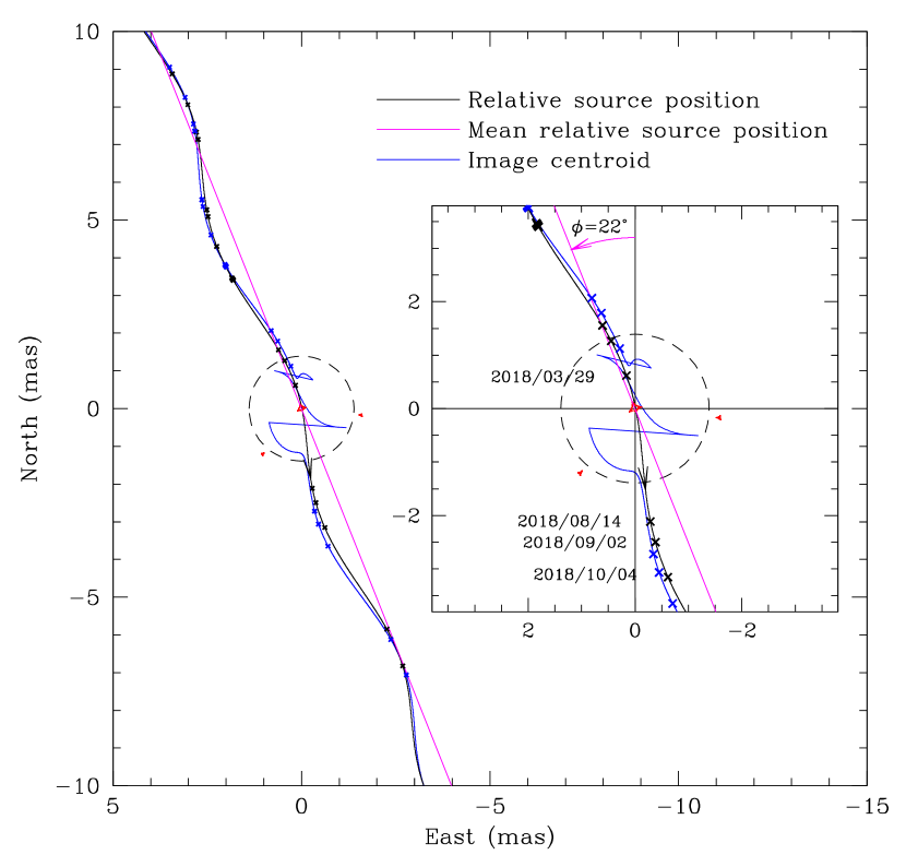
Figure 9.— Motions of the source (black curve) and image centroid (blue curve) predicted by the photometric lensing solution. The straight magenta line represents the relative lens-source motion. The points on the source and image-centroid curves represent the times of Gaia observations. Coordinates are centered at the barycenter of the lens and the abscissa and ordinate are aligned to the East and North directions.

We also check the validity of the lensing solution by computing the projected kinetic-to-potential energy ratio of the lens system. From the determined physical parameters $M$ and $a_{\perp}$ combined with the lensing parameters $s$, $ds/dt$, and $d\alpha/dt$, the ratio is computed by

$$\left({{\rm KE}\over{\rm PE}}\right)_{\perp}={(a_{\perp}/{\rm au})^{3}\over 8\pi^{2}(M/M_{\odot})}\left[\left({1\over s}{ds/dt\over{\rm yr}^{-1}}\right)^{2}+\left({d\alpha/dt\over{\rm yr}^{-1}}\right)^{2}\right]\sim 0.09.$$ (12)

In order for the lens to be a gravitationally bound system, the ratio should meet the condition of $({\rm KE}/{\rm PE})_{\perp}\leq{\rm KE}/{\rm PE}\leq 1.0$. The estimated kinetic-to-potential energy ratio satisfies this condition. In Table 4, we summarize the determined physical lens parameters.

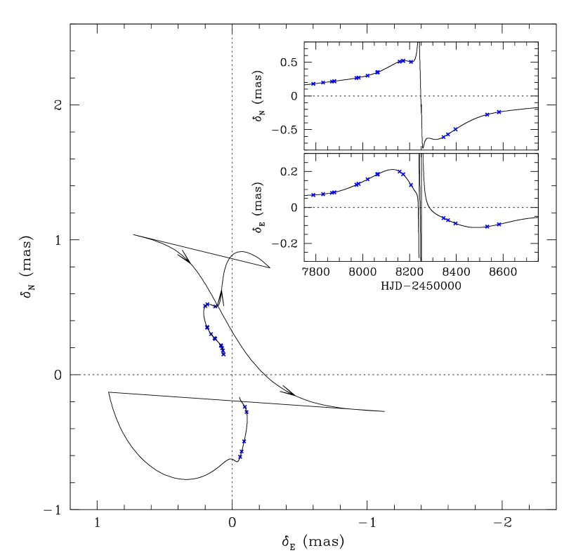
Figure 10.— Shift of the image centroid with respect to the unlensed source position. The two insets show the north and east components of the centroid shift vector as a function of time.

Given that the distance to the lens is small, the lens might comprise an important fraction of the blended light, e.g., OGLE-2017-BLG-0039 (Han et al., 2018b). We check this possibility by inspecting the agreement between the positions of the lens and blend in the CMD. In Figure 8, we place the locations of the blend and lens. The lens location is estimated based on the mass and distance. Considering the close distance to the lens, we assume that the lens experiences $\sim 1/3$ of the total extinction and reddening toward the bulge field of $A_{I}\sim 1.26$ and $E(V-I)\sim 1.02$, respectively (Nataf et al., 2013). The estimated color and brightness of the lens are $(V-I,I)_{\rm L}\sim(2.3,19.8)$, while those of the blend are $(V-I,I)_{b}\sim(1.7,18.9)$. The lens is substantially fainter and redder than the blend and this indicates that the lens is not the main source of the blended light.

4. Prediction of Gaia Astrometric Measurements

A lensing phenomenon causes not only the magnification of the source brightness but also the change of the image positions. When a source star is gravitationally lensed, it is split into multiple images and the brightness and location of each image change with the change of the relative lens-source position. By employing the GRAVITY instrument of the Very Large Telescope Interferometer (VLTI), Dong et al. (2018) recently reported the first resolution of the two microlens images of a domestic microlensing event TCP J05074264+2447555 (Gaia Collaboration, 2018), which occurred on a nearby source star located within $\sim 1$–2 kpc of the Sun in the direction opposite to the bulge field. This demonstrates that resolving microlens images is possible provided that a source is bright enough for VLTI GRAVITY observations ($K\lesssim 10.5$ or $I\lesssim 12.8$ for an $I-K=2.3$ star). For OGLE-2018-BLG-0022, the event during the caustic crossings was brighter than this threshold magnitude, and thus the separate images could have been resolved from VLTI GRAVITY observations, but no such observation was conducted.

Without directly resolving the separate images, a binary lens can still be astrometrically constrained by measuring the positional displacement of the image centroid (Han, 2001). Compared to the direct image resolution, which requires a resolution of order mas, the centroid shift measurement can be done with Gaia, which has resolution lower than VLTI GRAVITY by two orders of magnitude. Actually, the source of the event OGLE-2018-BLG-0022 is in the second Gaia data release. We, therefore, predict the astrometric behavior of the image centroid motion based on the solution obtained from the analysis of the photometric data.

In Figure 9, we present the motions of the source (black curve) and the image centroid (blue curve) in the East-North coordinates. By the time of writing this paper, the field has been observed 73 times by Gaia since 2014/10/15 (${\rm HJD}^{\prime}\sim 6945$) and 4 forthcoming observations are scheduled until 2019/04/08 (${\rm HJD}^{\prime}\sim 8583$). We mark the positions of the Gaia observations on the curves of the source and image-centroid motions. The straight magenta line represents the mean relative lens-source proper motion, i.e., without parallax motion, which is heading toward south-west with an angle $\phi_{\rm helio}\simeq 22^{\circ}$ as measured North through East. In Figure 10, we present the shift of the image centroid with respect to the unlensed source position, $\delta$. In the two insets, we present the north and east components of $\delta$ as a function of time.

The expected signal-to-noise ratio of the astrometric centroid shift measurement is

$${S\over N}={\sqrt{\sum_{i=1}^{N_{\rm obs}}{\delta_{i}^{2}}}\over\sqrt{2}\sigma_{\rm 1D}}={3.04\,{\rm mas}\over 0.707{\rm mas}}=4.3,$$ (13)

where $\delta_{i}=(\delta_{N,i}^{2}+\delta_{E,i}^{2})^{1/2}$ is the astrometric deviation, and $\sigma_{\rm 1D}$ is the mean astrometric error of an individual Gaia measurement along its principle axis. We estimate $\sqrt{2}\sigma_{\rm 1D}=\sigma_{\pi}[N_{\rm meas}\langle\sin^{2}(\Delta l)_{\rm eclip}\rangle]^{1/2}$, where $\sigma_{\pi}=0.218\,{\rm mas}$ is the reported Gaia parallax error, $N_{\rm meas}=13$ is the number of Gaia epochs entering this measurement, and $[\langle\sin^{2}(\Delta l)_{\rm eclip}\rangle]^{1/2}=0.9$ is the RMS parallactic offset of the target as seen by Gaia at the times of the observations. Therefore, it is expected that the astrometric centroid shift can be reliably measured.

5. Conclusion

We analyzed the binary-lensing event OGLE-2018-BLG-0022. Thanks to the dense and continuous coverage with the high-quality photometry data from the ground-based observations combined with space-based Spitzer observations, we found a lensing solution including microlens-parallax and lens-orbital parameters without any ambiguity, leading to the unique determination of the physical lens parameters. The robust and unique solution and the relatively bright source enabled the prediction of astrometric lensing signals that could be confirmed from actual astrometric observations using Gaia.

References

- Alard & Lupton (1998) Alard, C., & Lupton, R. H. 1998, ApJ, 503, 325
- Albrow (2017) Albrow, M. 2017, MichaelDAlbrow/pyDIA: Initial Release on Github, doi: 10.5281/zenodo.268049
- Albrow et al. (2009) Albrow, M. D., Horne, K., Bramich, D. M., et al. 2009, MNRAS, 397, 2099
- An (2005) An, J. H. 2005, MNRAS, 356, 1409
- Batista et al. (2011) Batista, V., Gould, A., Dieters, S., et al. 2011, A&A, 529, 102
- Bensby et al. (2011) Bensby, T., Adén, D., Meléndez, J., et al. 2011, PASP, 533, 134
- Bessell & Brett (1988) Bessell, M. S., & Brett, J. M. 1988, PASP, 100, 1134
- Bond et al. (2001) Bond, I. A., Abe, F., Dodd, R. J., et al. 2001, MNRAS, 327, 868
- Bramich (2018) Bramich, D. M. 2018, A&A, 618, A44
- Bramich & Nielsen (2018) Bramich, D. M., & Nielsen, M. B. 2018, Acta Astron., 68, 183
- Calchi Novati et al. (2015) Calchi Novati, S., Gould, A., Yee, J. C., 2015, ApJ, 814, 92
- Claret (2000) Claret, A. 2000, A&A, 363, 1081
- Dominik (1998) Dominik, M. 1998, A&A, 329, 36
- Dominik (1999) Dominik, M. 1999, A&A, 349, 108
- Dominik et al. (2008) Dominik, M., Horne, K., Allan, A., et al. 2008, Astronomische Nachrichten, 329, 248
- Dong et al. (2009) Dong, S., Gould, A., Udalski, A., et al. 2009, ApJ, 695, 970
- Dong et al. (2018) Dong, S., Mérand, A., Delplancke-Ströbele, F., et al. 2018, arXiv:1809.08243
- Gaia Collaboration (2018) Gaia Collaboration: Brown, A. G. A., Vallenari, A., Prusti, T., et al. 2018, A&A, 616, A1
- Gaia Collaboration (2016) Gaia Collaboration, 2016, A&A, 595, A1
- Gould (1992) Gould, A. 1992, ApJ, 392, 442
- Gould (1994) Gould, A. 1994, ApJ, 421, L75
- Gould (2004) Gould, A. 2004, ApJ, 606, 313
- Griest & Safazadeh (1998) Griest, K., & Safazadeh, N. 1998, ApJ, 500, 37
- Han (2001) Han, C. 2001, MNRAS, 325, 1281
- Han et al. (2018a) Han, C., Calchi Novati, S., Udalski, A., et al. 2018, ApJ, 859, 82
- Han et al. (2018b) Han, C., Jung, Y. K., Udalski, A., et al. 2018, ApJ, 867, 136
- Han et al. (2016) Han, C., Udalski, A., Lee, C.-U., et al. 2016, ApJ, 827, 11
- Ioka et al. (1999) Ioka, K., Nishi, R., & Kan-Ya, Y. 1999, PThPh, 102, 98
- Jung et al. (2018) Jung, Y. K., Han, C., Udalski, A., et al. 2018, ApJ, 863, 22
- Kervella et al. (2004) Kervella, P., Thévenin, F., Di Folco, E., & Ségransan, D. 2004, A&A, 426, 29
- Kim et al. (2016) Kim, S.-L., Lee, C.-U., Park, B.-G., et al. 2016, JKAS, 49, 37
- Nataf et al. (2013) Nataf, D. M., Gould, A., Fouqué, P., et al. 2013, ApJ, 769, 88
- Paczyński (1996) Paczyński, B. 1996, Acta Astron., 46, 291
- Proft et al. (2011) Proft, S., Demleitner, M., & Wambsganss, J. 2011, A&A, 536, 50
- Refsdal (1966) Refsdal, S. 1966, MNRAS, 134, 315
- Sahu et al. (2014) Sahu, K., Bond, H. E., Anderson, J., & Dominik, M. 2014, ApJ, 782, 89
- Salim & Gould (2000) Salim, S, & Gould, A, 2000, ApJ, 539, 241
- Schneider & Weiss (1986) Schneider, P., & Weiss, A. 1986, A&A, 164, 237
- Shin et al. (2012) Shin, I.-G., Han, C., Choi, J.-Y., et al. 2012, ApJ, 755, 91
- Shin et al. (2017) Shin, I.-G., Udalski, A., Yee, J. C., et al. 2017, AJ, 154, 176
- Skowron et al. (2011) Skowron, J., Udalski, A., Gould, A., et al. 2011, ApJ, 738, 87
- Smith et al. (2003) Smith, M. C., Mao, S., & Paczyński, B. 2003, MNRAS, 339, 925
- Szymański et al. (2011) Szymański, M.K., Udalski, A., Soszyński, I., et al. 2011, Acta Astron., 61, 83
- Udalski (2003) Udalski, A. 2003, Acta Astron., 53, 291
- Udalski et al. (2015) Udalski, A., Szymański, M. K., & Szymański, G. 2015, Acta Astron., 65, 1
- Yoo et al. (2004) Yoo, J., DePoy, D. L., Gal-Yam, A., et al. 2004, ApJ, 603, 139
- Zhu et al. (2015) Zhu, W., Udalski, A., Gould, A., et al. 2015, ApJ, 805, 8