Determining the physical conditions of extremely young Class 0 circumbinary disk around VLA1623A

Abstract

We present detailed analysis of high resolution C¹⁸O (2-1), SO ($8_{8}$-$7_{7}$), CO (3-2) and DCO⁺ (3-2) data obtained by the Atacama Large Millimeter/sub-millimeter Array (ALMA) towards a Class 0 Keplerian circumbinary disk around VLA1623A, which represents one of the most complete analysis towards a Class 0 source. From the dendrogram analysis, we identified several accretion flows feeding the circumbinary disk in a highly anisotropic manner. Stream-like SO emission around the circumbinary disk reveals the complicated shocks caused by the interactions between the disk, accretion flows and outflows. A wall-like structure is discovered south of VLA1623B. The discovery of two outflow cavity walls at the same position traveling at different velocities suggests the two outflows from both VLA1623A and VLA1623B overlays on top of each other in the plane of sky. Our detailed flat and flared disk modeling shows that Cycle 2 C¹⁸O J = 2-1 data is inconsistent with the combined binary mass of $0.2\,M_{\odot}$ as suggested by early Cycle 0 studies. The combined binary mass for VLA1623A should be modified to $0.3\sim 0.5\,M_{\odot}$.

1 Introduction

Around 50 percent of solar mass stars form in multiple systems (Raghavan et al., 2010). Multiplicity fraction increases for higher mass stars (Sana, & Evans, 2011). These multiple systems are formed in the early stage of star formation via three processes: turbulent fragmentation, thermal fragmentation of rotating cores, and disk fragmentation. Turbulent and thermal fragmentation occurs at relatively large scales, forming wide binaries with separation of order 1000 AU or larger. (Padoan, & Nordlund, 2002; Offner et al., 2010; Inutsuka, & Miyama, 1992; Burkert, & Bodenheimer, 1993; Boss, & Keiser, 2014; Pineda et al., 2015). As for the disk fragmentation, it is believed to be one of the primary processes for forming close ($\sim$ 100 AU) binaries (Takakuwa et al., 2012; Tobin et al., 2013).

Previous observations have found many circumbinary disks (Takakuwa et al., 2012; Tobin et al., 2013; Dutrey et al., 2014, 2016; Chou et al., 2014; Tang et al., 2014, 2016). Near-infrared surveys of Class I sources have found that around 15 out of 88 targets have binary separations between 50 to 200 AU (Connelley et al., 2008; Duchêne et al., 2007). Very Large Array survey of 94 known protostars in Perseus molecular clouds have found that Class 0 have significant higher multiplicity fraction (MF$=0.57\pm 0.09$) as compared to Class I sources (MF$=0.23\pm 0.08$)(Tobin et al., 2016). Submillimeter Array (SMA) studies of 33 Class 0 protostars in the nearby molecular clouds also found the multiplicity fraction (MF$=0.64\pm 0.08$) to be two times larger than Class I sources (Chen et al., 2013). Since disk fragmentation requires massive gravitationally unstable disks, close binary and multiplicity systems are expected to form in the early phase of star formation. Thus understanding the gas dynamics in extremely young Class 0 protobinary disk is crucial for testing binary formation theory.

Disk formation in the Class 0 phase attracted a lot of attention over the last 10 years and it remains an important unsolved problem for star formation. Numerical models simulating the collapse of a magnetized envelope with the assumption of ideal magnetohydrodynamics (MHD) show that disk formation is hindered by magnetic braking effects (Mellon, & Li, 2008). One solution proposed is that magnetic braking efficiency can be reduced if the rotation axis is misaligned with the magnetic field direction (Hennebelle, & Ciardi, 2009). Moreover, non-ideal MHD effects on disk formation have also been explored. Recently, 3D non-ideal MHD simulations have been carried out and a disk around 5 AU is formed at the end of the first core phase (Tomida et al., 2015). In the recent analytical study carried out by Hennebelle et al. (2016), a relationship between disk radius and magnetic fields in the inner part of the core is found. The weak dependence of various relevant quantities suggests that Class 0 disks have a typical disk size $\sim 18$ AU (Hennebelle et al., 2016).

An alternative solution to magnetic braking effects is turbulence. Santos-Lima et al. (2012, 2013) suggests that turbulence reconnection in disks is associated with the loss of magnetic flux which reduces the magnetic braking efficiency. In contrast, Seifried et al. (2015) have shown even with mild sub-sonic turbulence motion together with disorder magnetic field is enough for the formation of Class 0 Keplerian disks without the need for the loss of magnetic flux. In their simulations they found that both the accretion of mass and angular momentum is highly anisotropic.

Numerical simulations tend to have difficulties in explaining how the observed large Class 0 disks grow in size and possibly fragment. A well-studied Class 0 candidate, HH212 is found to have a Keplerian disk within the 44 AU centrifugal barrier (Lee et al., 2017). The Keplerian disk of Class 0 protostar L1527 has a disk radius of 74 AU and the scale height at 100 AU is 48 AU (Aso et al., 2017; Tobin et al., 2013). As for VLA1623A, the Keplerian rotating disk size is fitted to 150 AU using C¹⁸O as a tracer (Murillo et al., 2013). These observational results show Class 0 disks with varying disk sizes and structures. The discovery of large ($>$ 70AU) Class 0 rotationally supported disks, L1527 and VLA1623A, provide possible candidates to study disk fragmentation around Class 0 sources. Not much is known about how large rotationally supported disks are formed, and what factors influence their formation.

Figure 1: VLA1623 0.88 mm continuum image. The Class 0 source, VLA1623A is resolved into 2 sources, VLA1623A1 and VLA1623A2. The red ellipse marks the beam size.

VLA1623-2417 (VLA1623 hereafter) is a triple non-coeval protostellar system, located at 120$\pm$4.5 pc away in cloud $\rho$ Ophiuchus A (Andre et al., 1993; Loinard et al., 2008; Ortiz-León et al., 2017). The system consists of three components: VLA1623A (Class 0 source), VLA1623B (younger than VLA1623A, possibly a transition between starless core and Class 0) (Santangelo et al., 2015), and VLA1623W (Class 1) (Murillo, & Lai, 2013). Recent high angular resolution ($\sim$0$\farcs$16) 0.88 mm continuum data reveals that VLA1623A is in fact a binary denoted as VLA1623A1 and VLA1623A2 in Figure 1, and the Keplerian disk previously discovered is a circumbinary disk (Harris et al., 2018). The plane of sky separation between the VLA1623A1 and VLA1623A2 is around 0$\farcs$2, which corresponds to a physical scale of 24 AU. Unfortunately, our Cycle 2 C¹⁸O (J = 2-1) data with beam size 0$\farcs$5 cannot resolve the two sources (C¹⁸O Moment maps shown in Figure 2).

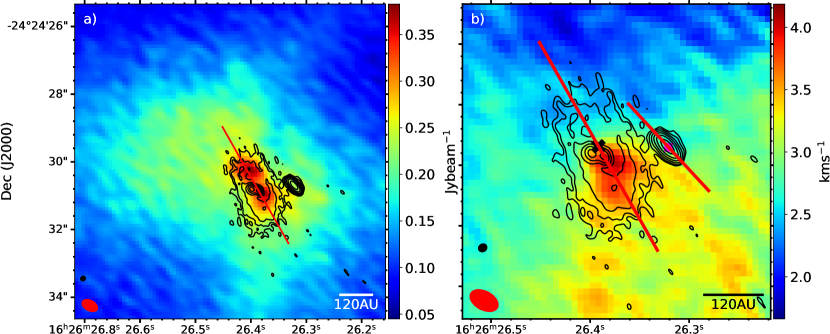
Figure 2: (a).VLA1623 0.88 mm continuum (contours) overlaid on the Briggs -1.0 weighted C¹⁸O integrated intensity map (color). The color represents the C¹⁸O J = 2-1 integrated intensity map (moment 0) using combined data from ALMA 12m array and 7m array. The black contours are 0.88 mm continuum data in steps of 3 $\sigma$, 5 $\sigma$, 10 $\sigma$, 20 $\sigma$, 40 $\sigma$, 80 $\sigma$, where $\sigma=5\times 10^{-4}$ Jy beam^-1. The red line indicates the location of the position velocity cuts used in this study (PA = 209.82^∘, centered at VLA1623A ($\alpha$(J2000) = 16^h26^m26$\fs$390, $\delta$(J2000) = –24°24′30$\farcs$688); PA=222.80^∘, centered at VLA1623B ($\alpha$(J2000) = 16^h26^m26$\fs$305, $\delta$(J2000) = –24°24′30$\farcs$705)). (b). VLA1623 0.88 mm continuum (contours) overlaid on the Briggs -1.0 weighted C¹⁸O intensity weighted velocity map (color). VLA1623A and B’s position are marked with a cross and a square, respectively.

Table 1: Summary of the observational data used in the analysis

				Maximum	Channel
Line	Transition	$\nu$	Beam Size	Recoverable	Widths	Rms noise	PI
		(GHz)	($\farcs$)	Scale ($\farcs$)	(kms-1)	(mJy beam-1)
CO	3-2	345.79599	$0\farcs 99\times 0\farcs 59$	$4\farcs 33$	0.0529	11	Cheng-Han Hsieh
C18O	2-1	219.56036	$0\farcs 52\times{0\farcs 31}$	$23\farcs 26$	0.0832	9
			$1\farcs 10\times 0\farcs 89$	$23\farcs 26$	0.0208	18	Shih-Ping Lai
			$0\farcs 51\times 0\farcs 31$	$23\farcs 26$	0.0208	14
DCO+	3-2	216.11402	$0\farcs 51\times 0\farcs 31$	$23\farcs 26$	0.085	5	Shih-Ping Lai
SO	$\nu=0$,	344.31061	$1\farcs 11\times 0\farcs 76$	$3\farcs 9$	0.212	20	Victor
	$J=8_{8}-7_{7}$						Magalh$\tilde{a}$es
Continuum	…	336.50000	$0\farcs 13\times 0\farcs 12$	$0\farcs 88$	53309.11	0.5	Leslie Looney
Total Power Array	…	219.56036	$29\farcs 67\times 29\farcs 67$	427$\farcs$86	0.0208	500	Shih-Ping Lai

With the increase of antennas and the UV-coverage, Cycle 2 data picks up significantly more C¹⁸O emission than Cycle 0 observations shown in Figure 3. VLA1623A, being one of the youngest protobinary disks ever discovered is thus the perfect candidate to study disk fragmentation around Class 0 sources.

In what follows, in Section 2 we discuss the data used in this analysis. In Section 3.1 we compare Cycle 0 and Cycle 2 C¹⁸O data and highlight major emission components that would be further explored. In Section 3 we present our main results of large scale emission fitting, dendrogram analysis (Cheong et al. 2019; submitted), flat and flared disk modeling, and accretion shocks analysis. In Section 4, we summarized the physical conditions of the VLA1623A circumbinary disk and its surrounding environment. In Section 5, we give our conclusions.

2 Observations

2.1 CO

We observed the CO ($J\,=\,3-2$) emission with Atacama Large Millimeter/submillimeter Array (ALMA) in Cycle 6 with pointing coordinates ($\alpha$(J2000) = 16^h26^m26$\fs$390, $\delta$(J2000) = –24°24′30$\farcs$688). The observation was taken on 2019 March 15 using 47 antenna of 12 m array in C34-1 compact configuration (project ID: 2018.1.00388S, PI: Chenghan Hsieh). The total on-source integration time is 10 minutes sampling baseline ranges between 15.1 $\sim$ 360.6 m. ALMA pipeline and Common Astronomy Software Applications (CASA) version 5.4.0-70 is used to calibrate the visibility data with J1924+2914 as the calibrator for bandpass and flux calibration and J1625+2527 for phase calibration. We used CASA CLEAN task with briggs 0.5 weighting and Hogbom as deconvolver for imaging. The resulting image has a beam size of 0$\farcs$99 $\times$ 0$\farcs$59 (P.A. = -84.8°) with rms noise level at 11 mJy beam^-1and velocity resolution at 0.0529  kms^-1.

2.2 C¹⁸O

C¹⁸O ($J=2-1$) were observed with ALMA in Cycle 2 with 12  m array configuration C34-5 and C34-1 (project ID: 2013.1.01004.S, PI: Shih-Ping Lai). We also include the 7m Atacama Compact Array (ACA) (hereafter 7m array) and Total Power Array of ACA in our analysis. The 12m array data and 7m array data are combined via the CASA task CLEAN with a weighting parameter of Briggs -1.5, Briggs -1.0, and a natural weighting. These maps are used for identifying accretion flows, comparing with ALMA C¹⁸O Cycle 0 data, and analysis of disk motion respectively.

For the Briggs -1.5 weighting, the UV taper range is $0\farcs 25$. The resulting C¹⁸O (J = 2–1) channel map has a resolution of $1\farcs 1\times 0\farcs 89$ (P.A. = $36.8^{\circ}$) with rms noise level at 18 mJy beam^-1. The velocity resolution is 0.0208 kms^-1 with rest frequency at 219.56036 GHz (corresponding to a system velocity of 4.0 kms^-1 away in the line of sight). The low resolution data is used for the dendrogram analysis and for identifying large structures around the circumbinary disk VLA1623A.

For the natural weighted data, Hogbom algorithm is used for the deconvolution process resulting the resolution of $0\farcs 52\times 0\farcs 31$ (P.A. = $87.89^{\circ}$) with rms noise level at 9 mJy beam^-1. The velocity resolution of 0.0832 kms^-1 is used to achieve a higher signal to noise ratio for disk modeling.

For comparison purposes, Briggs -1.0 weighting with UV taper range $0\farcs 25$ is applied to the Cycle 2 C¹⁸O data to achieve resolution $0\farcs 51\times 0\farcs 31$ (P.A. = $61.83^{\circ}$) with rms noise level at 14 mJy beam^-1. The velocity resolution is 0.0208 kms^-1. This data set is used to compare with Cycle 0 observation in Figure 3.

The C¹⁸O mean velocity map (Figure 2 b.) shows a rotating disk around VLA1623A. In this study, all the position-velocity (PV) diagrams will be aligned along the red line in Figure 2. The combined natural weighted C¹⁸O data for 12m array configuration C34-5 (baseline range $18.9\sim 1090$ m), C34-1 (baseline range $14.2\sim 347.3$ m), and 7m array (baseline range $7.1\sim 48.9$ m) data will be used in the analysis.

As for the Total Power Array data, the angular resolution is $29\farcs 67\times 29\farcs 67$ (P.A. = $0.0^{\circ}$) with rms noise level at 0.5 Jy beam^-1. The script provided by ALMA Regional Center (ARC) is used to calibrate and reduce the data. The Total Power Array data would be used to identify the large scale emission in the foreground as well as the background of the VLA1623A circumbinary disk.

2.3 Continuum data

We use the high resolution continuum data from the ALMA Archive (project ID: 2015.1.00084.S, PI: Leslie Looney) see Table 1. The observation is done in Band 7 with an integration time of 4798 seconds. The continuum data is prepared by using CASA task CLEAN with uniform weighting. The synthesized beam is $0\farcs 13\times 0\farcs 12$ (P.A. = $31.00^{\circ}$) with rms noise level at 0.5 mJy beam^-1.

2.4 DCO⁺$J=3-2$ data

The DCO+ data used in this paper is from ALMA Cycle 2 observation in Band 6 of the 12m array combined with the observation from the 7m array (project ID: 2013.1.01004.S, PI: Shih-Ping Lai). The data is prepared by the CASA task CLEAN with a weighting parameter of robust -0.5, and the UV taper range is set to 1$\farcs$0. The rms noise level of DCO+ data is $5$ mJy beam^-1 and the synthesis beam size is $0\farcs 51\times 0\farcs 31$ (P.A. = $63.05^{\circ}$). The velocity resolution of DCO⁺data is 0.085 kms^-1.

2.5 SO ($\nu=0,J=8_{8}-7_{7}$) data

In this paper, we present the results of the newly released ALMA Cycle 4 SO $\nu=0,J=8_{8}-7_{7}$ archival data (project ID: 2016.1.01468.S, PI: Victor Magalhaes) to trace accretion shocks (See Table 1). The observation is carried out by ALMA on March 4 in 2017 with a maximum UV baseline of $\sim$ 250 m. The data is calibrated by the ALMA calibration script, and the imaging is carried out via the CASA task CLEAN with a weighting parameter of robust 0.0. The resulting synthesized beam has an angular resolution of $1\farcs 11\times 0\farcs 76$ (P.A. = $82.59^{\circ}$) with rms noise level at 20 mJy beam^-1. The largest recoverable angular scale is around $3\farcs 5$. The spectral resolution is 0.212 kms^-1, and the SO ($\nu=0,J=8_{8}-7_{7}$) data have a line width larger than 8 kms^-1 resulting in a line width to channel width ratio $\sim$ 37.

3 Analysis

3.1 The comparison between Cycle 0 and Cycle 2 data

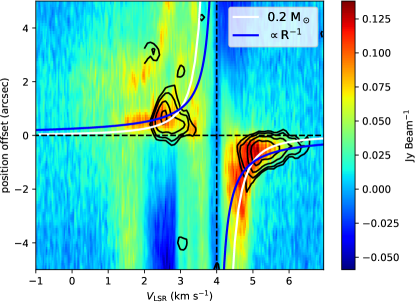
Figure 3: VLA1623A C¹⁸O J = 2-1 PV diagram for Briggs -1.0. The black contours marked the ALMA Cycle 0 C¹⁸O J=2–1 data, and the color background represents ALMA Cycle 2 C¹⁸O J=2–1 data. The blue line represents the infall velocity profile with conserved specific angular momentum. The white line represents the Keplerian rotation profile with a central mass of 0.2 $M_{\odot}$.

Figure 3 shows the comparison between the Cycle 0 (project ID: 2011.0.00902.S, PI: Nadia Murillo) and Cycle 2 (project ID: 2013.1.01004.S, PI: Shih-Ping Lai) ALMA data. In the Cycle 2 data shown as color background, we identified a high-velocity blue-shifted emission around 1.5 kms^-1, and the red-shifted emission extends to 4$\farcs$0. These features do not show in the Cycle 0 observations because there is not enough sampling in the short baselines.

Cycle 0 consists of only 16 antennae with a maximum baseline of $\sim$ 400 m. The beam-size is around $0\farcs 79\times 0\farcs 61$ with velocity resolution of 0.0833 kms^-1 (Murillo et al., 2013). The largest recoverable angular scale is around $2\farcs 46$. In comparison, Cycle 2 observations have increased sensitivity from the larger number of antennas and larger recoverable scale. More C¹⁸O emission is recovered. Thus, the previous disk size and the structure of VLA1623A Keplerian disk needs to be reanalyzed.

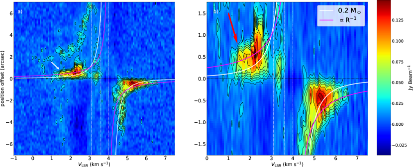
Figure 4: (a). Position-Velocity (PV) cut of the natural weighted C¹⁸O J = 2-1 ALMA Cycle 2 VLA1623A Keplerian disk. Centered at VLA1623A with position angle 209.82^∘ degrees. The magenta line represents the infall velocity profile with conserved specific angular momentum. The white line represents the Keplerian rotation profile with a central mass of 0.2 $M_{\odot}$ The white arrow marks the position of a gap between accretion flow and the Keplerian disk. The vertical white dotted lines mark the velocity of the major filtered out large scale emission (b). The zoomed in image of (a). Note the red arrow highlights a super-Keplerian rotation region.

3.2 Position velocity diagram

To study the gas kinematics, we create position-velocity (PV) diagrams centered at VLA1623A along the red line shown in Figure 2 ($\alpha$(J2000) = 16^h26^m26$\fs$390, $\delta$(J2000) = –24°24′30$\farcs$688), PA = 209.82^∘) with central velocity at 4.0 km s^-1. Since the binary separation is within our beam-size, the results are the same when we shift the PV cut from one component to the other. Thus we select the center of C¹⁸O emission for our PV diagrams. From the rotation curves, the Keplerian rotation with a central star mass 0.2 M_⊙ and an inclination angle of $55^{\circ}$ fits the PV data generally quite well. This is consistent with the results of Murillo using Cycle 0 data. Thus we first set the combined mass for the VLA1623A1 and VLA1623A2 binary to be 0.2 M_⊙ for flat and flared disk modeling.

In the high-velocity blue-shifted part we observed a strong emission above the Keplerian rotation white line (marked by a red arrow in Figure 4). The emission between 1.5 kms^-1 and 2.0 kms^-1 is reasonably well fitted with the infall line (with conserved angular momentum). This feature has not been seen in the Cycle 0 observation. The scaling of the conserved angular momentum line was set such that the cross over point with the Keplerian curve is located at the centrifugal radius of the disk. The corresponding specific angular momentum is 120 AU kms^-1. The detailed estimation of centrifugal radius is shown in Appendix A.

Is this high-velocity blue-shifted component part of the Keplerian disk? Is it due to a flared Keplerian disk with projection effects? Or is it accretion flows or other large structures in the line of sight? To determine the nature of this super-Keplerian rotation component we will conduct an analysis to identify large scale cloud emission, accretion flows, large scale structures, and the flared Keplerian disk.

3.3 Large scale emission around VLA1623

Figure 5: Gaussian fit of a total power spectrum of VLA1623. The black line represents the observational data for the Total Power Array, and the color lines represent the Gaussian fitting result.

Table 2: Total Power Spectrum fitting results (Large-scale emission)

Number	Velocity	Amplitude	Widths
	(kms-1)	(Jy)	(kms-1)
1	3.632	320.19	0.2782
2	3.996	153.11	0.1117
3	3.104	152.29	1.3790
4	2.561	19.87	0.0164
5	2.029	10.04	0.0348
	$\sigma=0.353(Jy)$	$\chi^{2}=9401.49$	$\chi^{2}/dof=29.29$

The total power spectrum data is used to determine the strength and velocities of the gas corresponding to the large-scale emission around the VLA1623. We did not combine the Total Power data with the 12m+7m array data in order to separate the compact disk emission from the large-scale cloud emission. In Figure 5, five Gaussian functions are used to fit the total power spectrum with the best fit result shown in Table 2. The main component identified from the Total Power Array (3.632 km s^-1) is closed to the system velocity and has intensity significantly larger than the other extended emission. We therefore associate the maximum component at velocity 3.632 km s^-1 as the cloud emission of the VLA1623 system. In Figure 3 at the system velocity 4.0 kms^-1 the C¹⁸O suffers a huge absorption and this is consistent with our Gaussian fitted extended emission component 2 shown in Figure 5. The coincident of vertical gaps in the PV diagrams and the Total Power components suggest these vertical gaps are resulted from the spatial filtering of extended emission. In all the C¹⁸O PV diagrams, we combined both the 12m array and 7m array to have maximum recoverable scale up to $\sim$23$\farcs$3 ($\sim$2760 AU). The disk emission and accretion flows are well covered in this range. Total Power Array traces extended emission at scales from $\sim$29$\farcs$7 ($\sim$3350 AU) to $\sim$427$\farcs$9 ($\sim$51350 AU). Any emission only observed in the Total Power Array is unlikely to be originated from the compact disk or accretion flows.

For other minor components located at velocities 3.104, 2.029, and 2.561 kms^-1, their physical origins and whether or not they are part of the VLA1623 system are unclear. Furthermore, all the filtered large scale emission in the PV diagrams including the central envelope are located in the blue-shifted region which is consistent with the preliminary estimations done by Murillo et al. (2013).

The Total Power data (large scale emission) is not included in the flat and flared disk models (Section 3.5 and 3.6). Since large scale emission corresponds to scales much larger than the disk or accretion flows, they are unlikely originate from the disk emission, and the low spatial resolution of data would bias the modeling. The purpose of this Total Power data fitting is to identify the velocity of large scale emission. When comparing the data with models, we will avoid these components.

3.4 Using Dendrograms to identify Accretion flows and set constraint on disk size

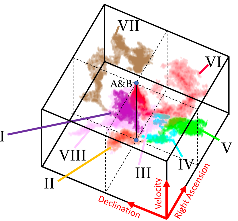
Figure 6: 3D Dendrogram around VLA1623 system. The C¹⁸O large structures are labeled with Roman numbers. The central black solid line marked the position of VLA1623A and VLA1623B in the PPV cube. VLA1623A and VLA1623B are very close to each other with separation within the blue dot. The 3D image is made by using GLUE visualization software (Beaumont et al., 2014). For the detailed analysis of dendrograms please see Cheong et al. (2019; submitted).

Figure 7: VLA1623A and blue-shifted accretion flow I channel maps. The color represents the C¹⁸O J = 2-1 emission (Briggs -1.5) identified by the dendrogram algorithm. The dendrogram corresponds to the Purple component (accretion flows and disk) in Cheong et al. (in prep.)’s paper. The magenta contours are 0.88 mm continuum data. The contours are in steps of 3 $\sigma$, 5 $\sigma$, 10 $\sigma$, 20 $\sigma$, 40 $\sigma$, 80 $\sigma$ , where $\sigma=5\times 10^{-4}$ Jy beam^-1).

A Class 0 protostar is actively accreting and is still deeply embedded in the envelope (Seifried et al., 2015). With infalling streamers feeding material from the envelope onto the circumbinary disk and outflows, it is challenging to identify disks around Class 0 sources. In order to determine the disk size in a Class 0 source, we need to identify outflows, envelope, accretion flows and other large scale structures. Outflows have been observed in ¹²CO by (Andre et al., 1990; Dent et al., 1995; Yu & Chernin, 1997). The envelope, which is located at 3.6 km s^-1 fitted by the total power spectrum, can be separated out from the rest of the components in velocity domain.

The C¹⁸O traces both the rotational disk and accretion flows around it. The dendrogram algorithm is used to identify the connected structures in the position-position-velocity (PPV) space (Cheong et al. 2019; submitted; see Figure 6). The algorithm identifies in total 8 major branches (local maximum) labeled in Figure 6. In additional to the 6 major branches found in Cheong et al. (2019; submitted), we found another 2 large structures, blue-shifted III and VIII component, connected to the VLA1623A circumbinary disk. In the following sections, we use SO as a shock tracer to identify the interactions between accretion flows and the circumbinary disk (See Table 3, Figure 19).

Besides the blue-shifted III and VIII component, Cheong et al. (2019; submitted) further compared the data with the CMU model (Ulrich, 1976; Cassen, & Moosman, 1981), a rotating collapse model with conserved specific angular momentum, and found that the red-shifted VI component and blue-shifted I component are accretion flows connected to the central Keplerian disk (channel maps shown in Figure 7 & Figure 8).

Figure 7 shows the channel maps of the blue-shifted I component identified by the dendrogram. The 0.88 mm continuum data is shown as the magenta contours which mark the location of the VLA1623A circumbinary disk and VLA1623B. Inside the magenta contours, the C¹⁸O emission shows the blue-shifted I accretion flows are faintly connected to the central disk. The drop of C¹⁸O intensity between the disk and large structure I indicates a clear gap around 120 AU exists between the large scale structure and the Keplerian disk. The Keplerian disk is constrained to roughly 180 AU from the blue-shifted channel maps.

Figure 8 shows the channel maps of the red-shifted accretion flow VI connected to the central disk. In the velocity channels between 4.17 to 5.00 kms^-1, the accretion flow is well mixed with the disk and the C¹⁸O emission extends to 6$\farcs$0 ($\sim$ 500 AU). Only in the high-velocity channels ( $>$ 5.1 kms^-1), the C¹⁸O emission traces the Keplerian disk without any contamination from the accretion flow. High-velocity channels are not contaminated by accretion flows, but they only provide the information in the inner region in the Keplerian disk. Thus the disk size can’t be determined by the red-shifted channels.

From the rotation curves in Figure 4, we deduce the motion of the disk is Keplerian. And hence without loss of generality, we can assume the disk is axially symmetric and use the blue-shifted side to constrain the disk size. We select the continuum level such that the edge of the disk matches the boundary of the gap in Figure 7. Therefore, the circumbinary disk size is constrained to be 180 AU. Furthermore, the extended emission between 4 kms^-1 and 5 kms^-1 in Figure 3 is likely a mixture of accretion flow and disk components. We will explore this more in the following sections. More technical details of dendrogram data preparation and accretion flows modeling can be found in Cheong et al. (2019; submitted)’s paper.

Figure 8: VLA1623A and red-shifted accretion flow VI channel maps. The color represents the C¹⁸O J = 2-1 (Briggs -1.5) emission identified by the dendrogram algorithm. The dendrogram corresponds to the Red component (accretion flows and disk) in Cheong et al. (in prep.)’s paper. The magenta contours are 0.88 mm continuum data. The contours are in steps of 5 $\sigma$, 40 $\sigma$, where $\sigma=5\times 10^{-4}$ Jy beam^-1.

3.5 Flat Disk Model

We first model the ALMA Cycle 2 C¹⁸O J = 2–1 position-velocity (PV) diagram of the VLA1623A circumbinary disk with a Flat Keplerian disk model. The PV diagram are cut along the red line in Figure 2. The governing equations for the velocity, temperature, and column density profiles in the flat Keplerian disk are described as the following:

$$v(R)=\sqrt[]{\frac{GM_{*}}{R}}$$ (1)

$$T(R)=T_{0}\times\bigg{(}\frac{R}{100AU}\bigg{)}^{-0.5}$$ (2)

$$\Sigma(R)=\Sigma_{0}\times\bigg{(}\frac{R}{100AU}\bigg{)}^{-1}$$ (3)

For the column density at 100 AU ($\Sigma_{0}$), we adopted the number to be $6.173\times 10^{21}$ cm^-2, and the disk inclination angle is $55^{\circ}$ (Murillo et al., 2013). For temperature distribution we assume the temperature power law exponent to be -0.5, and we adopted a temperature of $\sim 30$ K at 100 AU based on the DCO⁺ 5-4/3-2 data (Murillo et al., 2018).

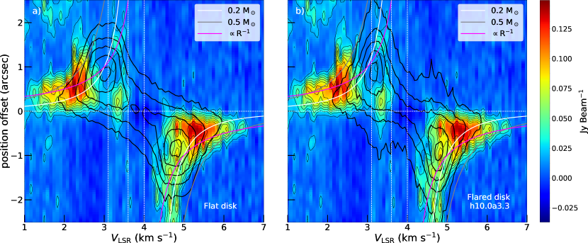
Figure 9: (a). Position velocity (PV) diagram of the VL1623A Keplerian disk overlaid with flat disk model contours. The color represents the PV diagram of the natural weighted C¹⁸O J = 2-1 emission centered at VLA1623A. The thick black contours outline the Flat Keplerian disk model in steps of 5 $\sigma$, 10 $\sigma$, 20 $\sigma$, 30 $\sigma$, 40 $\sigma$, 45 $\sigma$, 50 $\sigma$, where $\sigma=6\,$ mJy beam^-1. (b). Position-Velocity (PV) diagram of the VLA1623A Keplerian disk overlaid with the best fit flared disk model contours (vertical scale height $h_{0}=10.0$ and power law index $a=3.3$). The thick black contours outline the Flared Keplerian disk model in steps of 0.2, 0.4, 0.6, 0.8, 0.95 of the maximum flux in the model. In both panels, the white, gray and the magenta lines represent the Keplerian rotation curve with central star mass 0.2, 0.5 $M_{\odot}$ and an inclination angle of $55^{\circ}$. The infall velocity profile with conserved specific angular momentum respectively. The vertical white dotted lines mark the velocities of the major filtered out large scale emission. The color background represents the PV diagram of the natural weighted C¹⁸O J = 2-1 emission centered at VLA1623A and the thin black contours are plotted for 3 $\sigma$, 5 $\sigma$, 7 $\sigma$, 9 $\sigma$, 11 $\sigma$, 13 $\sigma$, 15 $\sigma$ with $\sigma=9$  mJybeam^-1.

A flat disk model is first generated using Equation 1, Equation 2, and Equation 3. A simple ray tracing radiative transfer calculation scheme assuming local thermal equilibrium (LTE) with a thermal broadening of 0.2 kms^-1 is used to generate the synthetic images in position-position velocity (PPV) space. Then the simulated disk is convolved with the ALMA telescope beam using CASA SimObserve and CASA SimAnalyze. The exact antenna setup for C34-1, C34-5 and two ACA observations are input into SimObserve to recreate the exact beam used in the observation.

From the PV diagram shown in Figure 9 a, we found the peak location of the flat disk model has a significant offset compared to the data. The flat disk model has a peak located at 0$\farcs$8 position offset while the observational data have a peak located at 0$\farcs$5 position offset in the red-shifted side. No emission was detected in the observational data corresponding to the flat disk model’s blue-shifted peak, and this is consistent with the filtering of the large scale emission at 3.1 km s^-1 fitted by the total power spectrum.

We plot both the infall with conserved angular momentum and Keplerian rotation curves in Figure 9 a. In the outer region of the disk, the white Keplerian line passes through the flat Keplerian disk model and the observation data on the red-shifted side for position offset within 2$\farcs$5. However, in the corresponding zoomed out PV diagram in Figure 4 a, for position offset greater than 2$\farcs$5 the white Keplerian rotation line clearly deviates from the data. Thus it is very likely the C¹⁸O long tail between 2$\farcs$5 to 5$\farcs$0 corresponds to materials at system velocity slowly infalling towards the circumbinary disk.

3.6 Flared Disk Model and the constraint of VLA1623 circumbinary disk’s vertical scale height

A more sophisticated 3D flared disk model is further developed to constrain the density profile and the physical structure of the circumbinary disk around VLA1623A. We followed the equations of Guilloteau & Dutrey to develop a 3D flared disk model (Guilloteau, & Dutrey, 1998; Yen et al., 2014). The density, velocity and temperature profile are given as the following:

$$v(R)={\bigg{(}{\frac{GM_{*}}{R}}\bigg{)}^{-v}}$$ (4)

$$T(R)=T_{0}\times\bigg{(}\frac{R}{100AU}\bigg{)}^{-q}$$ (5)

$$\rho(R)=\rho_{0}\times\bigg{(}\frac{R}{100AU}\bigg{)}^{-a}\times exp\bigg{(}-\frac{z^{2}}{2h(R)^{2}}\bigg{)}$$ (6)

And the scale height relationship is given as:

$$h(R)=h_{0}\times\bigg{(}\frac{R}{100AU}\bigg{)}^{b}$$ (7)

$h_{0}$ is the scale height of the circumbinary disk at 100 AU, and b is the flaring index. Assuming hydrostatic equilibrium, the scale height $b=1+v-q/2$ with $v=0.5,\,q=0.4$ for a theoretical flared Keplerian disk (Guilloteau et al., 2011). The value of b is set to 1.29, using the theoretical model of flared disk (Chiang, & Goldreich, 1997). The value of $a$ follows the $a=p+1+v-q/2=1.3+p$ , with p being the power law index of surface density $\Sigma=\Sigma_{0}r^{-p}$ (Guilloteau, & Dutrey, 1998). Considering the typical range for surface density power law $1\leq p\leq 2$ we explore the density power law index $a$ in the range between $2.0\sim 4.0$.

Figure 10: Position-Velocity (PV) diagram of the VLA1623A Keplerian disk overlaid with flared disk model contours (central binary mass: 0.2 $M_{\odot}$) for different vertical scale height $h_{0}$ and density power law $a$. The color represents the PV diagram of the natural weighted C¹⁸O J = 2-1 emission centered at VLA1623A and the thin black contours are plotted for 3 $\sigma$, 5 $\sigma$, 9 $\sigma$, 11 $\sigma$, 13 $\sigma$, 15 $\sigma$ with $\sigma=9$ mJybeam^-1. The brown contour marks the 7 $\sigma$ line used for model comparison. The thick black contours are from the Flared Keplerian disk model. The contours are in steps of 0.2, 0.4, 0.6, 0.8, 0.95 of the maximum flux in the model. The white and gray lines represent the Keplerian rotation curve with central star mass 0.2 and 0.5 $M_{\odot}$ and an inclination angle of $55^{\circ}$. The magenta line represents the infall velocity profile with conserved angular momentum.

In our simple flared disk model we set the C¹⁸O to H₂ ratio to be $1.7\times 10^{-7}$. The resolution of the model is $500\times 500\times 500$ with each pixel at the resolution of 0.72 AU. For the density profile, we normalized the $\rho_{0}$ such that the total mass of the circumbinary disk is 0.02 $M_{\odot}$ (Cheong et al. 2019; submitted). The disk size is set to be 180 AU in radius as constrained from the C¹⁸O data. The inclination angle is 55^∘ and the distance is at 120 pc (Loinard et al., 2008; Murillo et al., 2013).

We apply the RADMC-3D radiative transfer code on flared disk model to create synthetic images in 3D Cartesian geometries with channel width set to 0.060 kms^-1 (Dullemond et al., 2012). The synthetic images are then convolved with the ALMA telescope beam using CASA SimObserve and CASA SimAnalyze. Since we are interested in the density structure ($a$) and the vertical structure ($h_{0}$) of the flared circumbinary disk, we fixed the temperature $T_{0}$ to be 30K at 100AU based on the DCO⁺ data (Murillo et al., 2018).

Figure 10 display various flared disk models with different density power law index $a$ and the vertical scale height parameter $h_{0}$ for the red-shifted side of the disk. Comparing the models in Figure 10 and Figure 20 with observation data is very challenging. The total power spectrum reveals a huge large scale emission at velocity 4.0 kms^-1 (systematic velocity) and many more on the blue-shifted side. Therefore, in order to eliminate the contamination of the large scale cloud, foreground and background emission, we only model the red-shifted part on the right side of the line corresponding to system velocity 4.0 kms^-1. Furthermore, to avoid the contamination from the outer accretion flows, we only compare the data and model within the disk radius ($\leq$ 1$\farcs$5).

Isophote contours for each simulation model are plotted in order to compare the observational data with simulation models. Overall we run the parameters $h_{0}=1.0,\,2.5,\,5.0,\,10.0,\,15.0,\,25.0$ (AU) and $a=2.0,\,2.3,\,2.6,\,3.0,\,3.3,\,4.0$ for a total of 36 parameter combinations to examine how the central peak location changes when the scale height $h_{0}$ and the density power law index $a$ are varied.

In Figure 10 as the vertical scale height $h_{0}$ increases, the model’s peak (thick black contours) would shift towards the connecting bridge between blue-shifted and red-shifted region (system velocity 4 kms^-1, and offsets 0.0). As for the density power law index $a$, when $a$ increases the PV diagram would be stretched in the direction of the Keplerian rotation line (white line). This is because when $a$ increases, the extended part of the disk would be suppressed and the intensity peak would move closer to the disk center.

At first sight, the best fit model would be the one with density power law index $a=4.0$, and scale height $h_{0}=25.0$. The density power law index $a=4.0$ suggests the peak is very compact in the center of the circumbinary disk VLA1623A. In the very high velocity region $v>6.0$ kms^-1 and $v<2.0$ kms^-1 , the observation data deviates from the flared disk model and doesn’t follow the white Keplerian rotation line. This deviation suggests that an inner compact structure exists inside the VLA1623A circumbinary disk. To avoid the contamination from the inner super-Keplerian region when constraining the circumbinary disk properties, we only model the data outside the inner region ($\sim$0$\farcs$5 (60 AU)) where the inner structures of VLA1623A lies.

For the model with parameters $a=4.0,\,h_{0}=25.0$, we found the peak of the flared disk model has the same position offset ($\sim$ 0$\farcs$5) as the observation data but at a much lower velocity (4.9 kms^-1 as compared to 5.2 kms^-1). The peak of the flared disk model and observational data does not overlap suggests that the circumbinary disk does not have density power law index $a$ as large as 4.0. Instead, it has a relatively flatter density power law plus a compact inner structure within 60 AU from the disk center.

For density power law index $a$ less than 3.3, there are only minor differences when $a$ varies. The PV diagram overall is insensitive to parameter $a$. To prevent contamination of large scale emission and internal structures, we search for disk models with parameter $a\leq 3.3$, peak locations between 0$\farcs$5 $\sim$ 1$\farcs$5 in position offset, and have emission between $4.5\sim 4.9$ kms^-1.

Close inspection of the fitting reveals that when the vertical scale height $h_{0}$ equals to 25.0 AU, the models have peaks locate at velocity $4.5\sim 4.7$ kms^-1 on the red-shifted side. Most importantly, in all the $h_{0}=25.0$ models more than half of the peak area falls outside the $7\,\sigma$ (63 mJy brown line in Figure 10) line on the red-shifted side. This significant offset shows that the $h_{0}=25.0$ does not fit the data. For vertical scale height $h_{0}=15$ AU, the peak overlap area is around 20 % for model $h_{0}=15,\,a=2.6$, but around 70 % for $h_{0}=15,\,a=3.3$. Thus it cannot be completely ruled out. For vertical scale height $h_{0}$ less than or equal to 10 AU, the overlap region is more than 50 %. Therefore, we can only constrain the density power-law $a$ for the VLA1623A circumbinary disk to be $a\leq 3.3$ with the vertical scale height at 100 AU to be $h_{0}\leq 15\,$ AU.

It is important to highlight again that for all of the parameter sets, no model can perfectly fit the location of the peak in the PV diagram. Both flat and flared disk model does not produce peaks at the same location as the observational data. Changing vertical scale height can’t produce high-velocity peaks in the inner region of the Keplerian disk, and adjusting density power law only stretches the contours along the Keplerian rotational line. From the flat and flared disk modeling, we have shown that simple Keplerian rotation disk models with combined binary mass of 0.2 $M_{\odot}$ cannot fully explain the observational data.

3.7 Limitations and Degeneracy in Modelling

Modeling and constructing a coherent picture from the complex data set around the Class 0 source VLA1623 is difficult, as multiple physical processes (outflows, infalls, rotation, shocks) need to be taken into account, and a wide range of parameters can be adjusted. A careful and logical reasoning is required to connect the pieces and form the overall picture. In this section, we will discuss the limitations and the logical reasoning behind breaking the degeneracy in the modelling.

3.7.1 Important parameters and limitations of the disk modeling

Since the flared disk model is used to constrain disk properties (disk scale height and density power law index), the discussion of important parameters and limitations of the disk modeling will be focused on the flared disk model.

In total there are 10 parameters in the flared disk model: scale height, temperature profile (power law index and normalization), density profile (power law index and normalization), inner cutoff radius, disk inclination, disk size, combined binary mass, and distance. Two parameters, density profile (power law index) and scale height, are free parameters that are explored and constrained. The other 8 parameters and their effects on the PV diagram modeling (Figure 10) are listed below:

1. Temperature profile (power law index):

   The profile affects the position of the peak in the disk by stretching the peak along the Keplerian rotation line in the PV diagram. This is the second largest uncertainty in the modeling. It will be discussed more in § 3.7.2. However, we do not expect huge deviation from the theoretical flared disk model unless other heating or cooling mechanisms are present.

2. Temperature normalization at 100 AU:

   Affects the overall normalization of the flux. Does not change the peak position in PV diagram, therefore has no or little effect on the scale height and density power law modeling.

3. Density normalization (Disk mass):

   Affects the overall normalization of the flux. Also has little or no effect on the peak position in the PV diagram. It is constrained by normalizing the disk mass to 0.02 M_⊙ (Cheong et al. 2019; submitted).

4. Disk size:

   The gas disk size is $\sim 180$ AU constrained by the inner edge of the gap in Figure 4 and Figure 7. Disk size affects the spatial size of the model in the PV diagram. This parameter is well constrained by observation, and has uncertainty around half of the beam size ($\sim$30 AU).

5. inner cutoff radius:

   Since the disk is in Keplerian rotation, the closer to the protostar the faster it rotates. The inner cutoff radius would determine the velocity cutoff point in the PV diagram. To prevent artificial velocity cutoff at high velocity, small inner cutoff radius is chosen. In the inner region of the disk since the area decreases with smaller radius, the intensity drops rapidly at high velocity end of the PV diagram. Therefore, for small enough inner cutoff radius the velocity cuttoff would have little or no effect on the disk modeling. In the flared disk modeling, the inner cutoff radius is set to be 1 AU (cell size 0.72 AU). As for the flat disk model the inner cutoff radius is also 1 AU.

6. Disk inclination

   The inclination angle used in the modeling is 55^∘ (Loinard et al., 2008; Murillo et al., 2013). The PV diagram is aligned along the major axis of the disk, so the change in inclination would have no effects in the direction of position offset in the PV diagram. Inclination only affects the projection of velocity to the line of sight and stretches the model contours away or towards from the systematic velocity. Even for 5^∘ variation of inclination angle, the velocity stretching factor is less than 7 %. In Figure 10, for density power law index $a<3.3$ the peak velocity difference between vertical scale height $h=15$ AU and $h=25$ AU is $\sim 0.2$ kms^-1. The peak velocity of the $h=25$ AU models are located around 0.6 to 0.7 kms^-1 away from the systematic velocity. If the $h=25$ AU models are stretched by 7 %, the peak velocity would increase at most by $\sim 0.05$ kms^-1, which is still smaller than the $0.2$ kms^-1 difference used to distinguish accepted and non-accepted models. Thus disk inclination in our modeling would not change the result of flared disk modeling.

7. Combined binary mass

   Combined binary mass is the most important factor in the disk modeling. Not only will it significantly affect the results on flared disk modeling, it is also a possible explanation for the super-Keplerian rotation in the inner region of the disk. More in-depth discussion about the degeneracy of combined binary mass would be presented in § 4.1.

8. Distance

   In this paper, the distance of 120 pc (Murillo, & Lai, 2013) is used in the modelling instead of 137.3 pc (Ortiz-León et al., 2017). The physical scale would increase by a factor of 1.14 if the 137.3 pc distance is adopted. In Figure 10, for power law index $a<3.3$, the shape of the model peaks are elongated in the direction of position offset. One major difference between vertical scale height $h=15$ AU and vertical scale height $h=25$ AU is that the centers of the peaks are located at different velocities. Stretching the models by 14 % in position offset would make it harder to differentiate between the two, but it will not change the result of the flared disk modeling.

3.7.2 Degeneracy in Temperature and Density profile

Disk intensity profile is determined by both temperature and density. In this study, for the flared disk model we assumed a fixed temperature profile with a power law index of -0.4 based on the theoretical flared Keplerian disk model (Guilloteau et al., 2011). As for the normalization we fixed the temperature to 30 K at 100 AU based on the previous DCO⁺ modeling (Murillo et al., 2018).

Fixing the temperature profile greatly reduces the free parameters in the modelling. It is important to note that the temperature profile is based on a simple theoretical model and in reality the actual temperature profile might deviate from this fixed profile. If the power law index is varied with the overall temperature normalization fixed at 100 AU, you would expect the peak to move inward or outward depending on the power law index. In other words, the peak will move along the Keplerian rotation line in the PV diagram. This will affect the density and scale height modeling, making it even more difficult to break the degeneracy, but the model still won’t be able to reproduce the observed peaks which clearly deviates from the Keplerian rotation. Thus it is not a good explanation for the super-Keplerian motion.

It will, however, affect the result of scale height modeling. For a larger disk scale height, the peak will move closer to the position offset 0.0 (center of the disk) and towards the system velocity in the PV diagram. Adjusting the temperature power law index would further stretches the peak along the Keplerian line. The two completing effects combined would make it very difficult to break the degeneracy. Even so, we do not expect the temperature profile to deviate too much from the theoretical flared disk model unless additional heating or cooling processes are involved.

The better and more accurate way to break the temperature and density degeneracy is to use two C¹⁸O transitions to obtain the temperature profile and constrain it directly from observation instead of using the simple theoretical model. Future observation is needed to more accurately constrain the temperature profile of the VLA1623A circumbinary disk.

3.8 Accretion shocks around the circumbinary disk

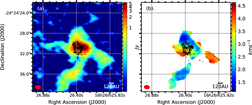
Figure 11: (a). SO intensity integrated map (Moment 0). The color represents the ALMA Cycle 4 SO $\nu=0,J=8_{8}-7_{7}$ data. The black contours are 0.88 mm continuum data. The contours are in steps of 3 $\sigma$, 5 $\sigma$, 10 $\sigma$, 20 $\sigma$, 40 $\sigma$, 80 $\sigma$ , where $\sigma=5\times 10^{-4}$ Jy beam^-1. (b). SO mean velocity map (Moment 1).

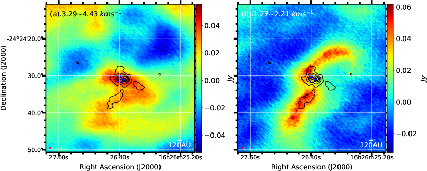
Figure 12: (a). C¹⁸O J = 2-1 intensity integrated map (Moment 0) between 3.29 kms^-1 and 4.43 kms^-1 for Briggs -1.0 weighted data. (b). C¹⁸O J = 2-1 intensity integrated map (Moment 0) between 1.27 kms^-1 and 2.21 kms^-1 for Briggs -1.0 weighted data. The color in both panels represent the C¹⁸O data. The black contours are ALMA Cycle 4 SO $\nu=0,J=8_{8}-7_{7}$ data. The contours are in steps of 0.025, 0.05, 0.1, 0.2, 0.4, 0.8 of the maximum intensity which is $8.5$ Jy beam^-1. The central blue contours are 0.88 mm continuum data in steps of 5$\sigma$, 40$\sigma$, where $\sigma=5\times 10^{-4}$ Jy beam^-1. The continuum data marked the position of the VLA1623A circumbinary disk and VLA1623B.

SO with sublimation temperature of 50 K is generally attached to dust grains. Observation of SO emission indicates that it comes from collisions or shocks that give enough energy to free SO into the gas phase. Previously SO emission has been used to trace shock fronts in another similar Class 0 disk system, L1527 (Sakai et al., 2014). In this section, we use SO as a shock tracer to understand the interactions between the accretion flows and the circumbinary disk.

Figure 11 a shows the SO $\nu=0,J=8_{8}-7_{7}$ Moment 0 map. A strong enhancement of SO molecules near the circumbinary disk and VLA1623B is apparent in the Moment 0 map and this indicates strong accretion shocks are created around VLA1623A circumbinary disk and VLA1623B. The SO emission shows 4 stream-like structures with two main streams to the west and south. The South stream has the strongest emission in all the streams and is connected to VLA1623B. The West stream corresponds to the red-shifted accretion flow VI identified by the dendrogram analysis using C¹⁸O, and the East stream corresponds to the blue-shifted accretion flow I in Figure 6 (Red and Purple Accretion flow respectively in Cheong et al. (2019; submitted)).

Figure 13: Intensity map of ALMA Cycle 4 SO ($\nu=0,J=8_{8}-7_{7}$, color), ALMA Cycle 6 CO (J = 3-2, red and white contours), and 0.88 mm continuum (black contours). The CO contours are in steps of 30 $\sigma$, 50 $\sigma$, 100 $\sigma$, 300 $\sigma$, where $\sigma=$ 11 mJy beam^-1 for CO. The red contours are red-shifted integrated CO emission between 8.80 kms^-1 to 17.1 kms^-1, and the white contours represent blue-shifted integrated CO emission between 5.20 kms^-1 to 8.59  kms^-1. The red circle marks the beam of the SO data, and the white circle represents the field of view for Band 7 CO observation.

Both the South and West stream connect to VLA1623B, and a strong emission of SO is detected on VLA16232B. The SO peaks at VLA1623B and the stream morphology suggests that on VLA1623B there exists violent shocks caused by the collision between B and the outer red-shifted accretion flow VI. As for the North and East streams, they connect to VLA1623A circumbinary disk on the map in the plane of sky. The North stream is much shorter than the South stream and this indicates the collision is much closer toward the VLA1623A and VLA1623B from the north. In the South stream, the peak locates around 7$\farcs$0 away south from the VLA1623A binaries.

Figure 11 b shows the mean velocity map (moment 1) of SO emission around VLA1623A circumbinary disk and VLA1623B. Notice that the system velocity of VLA1623A circumbinary disk is 4 kms^-1 and nearly all of the SO in Moment 1 map does not have a velocity greater than 4.4 kms^-1. The lack of red-shifted emissions in the North SO stream shows it corresponds to the blue-shifted accretion flow III (Figure 6) flow toward the circumbinary disk. The extended high velocity SO emission in the North stream is caused by the accretion shocks due to the collision between the circumbinary disk and accretion flow.

As for the South SO stream, it lies in the position corresponds to the red-shifted accretion flow VI (Fig. 8). However, the accretion flow VI traced by C¹⁸O is observed to be red-shifted and moving away from observer while the SO South stream is blue-shifted and moving in the opposite direction. For comparison between C¹⁸O and SO data, we plot the C¹⁸O J = 2-1 intensity integrated map (Moment 0) between 3.29 kms${}^{-1}\sim$ 4.43 kms^-1 in Figure 12 a and between 1.27 kms${}^{-1}\sim$ 2.21 kms^-1 in Figure 12 b with SO data display as black contours in both figures.

Figure 14: SO channel maps. The color represents the ALMA Cycle 4 SO $\nu=0,J=8_{8}-7_{7}$ data. The black contours are 0.88 mm continuum data in steps of 3 $\sigma$, 5 $\sigma$, 40 $\sigma$, 80 $\sigma$ , where $\sigma=5\times 10^{-4}$ Jy beam^-1.

In Figure 12 a, the C¹⁸O emission which corresponds to the materials at low blue-shifted velocity and at rest is much more extended than the Southern SO stream. C¹⁸O at rest are mostly distributed on the south side of the circumbinary disk and VLA1623B. Materials are piled up in the south, and this wall-like structure would be discussed in the next section.

One of the most prominent features in Figure 12 b is the Northern and Southern arm. The Northern C¹⁸O arm corresponds to the accretion flows III (See Figure 6). The Southern C¹⁸O arm has the same velocity range as the SO south stream and it overlays in the line of sight perfectly. From the dendrogram analysis carried out by Cheong et al. (2019; submitted), the Southern arm corresponds to the Structure II in Figure 6. Cheong et al. (2019; submitted) further carried out the CMU model analysis (Ulrich, 1976; Cassen, & Moosman, 1981), a rotating collapse model with conserved specific angular momentum, and found the blue-shifted component II does not match the CMU model. This indicates the materials in the South stream do not follow the infalling parabolic trajectories. From the dendrogram analysis and CMU fitting in Cheong et al. (2019; submitted) we concluded that the South SO stream of (Figure 11 a & b) corresponds to the materials with non-conserved specific angular momentum, possibly affected by outflows from the protostellar sources.

To confirm this interpretation, we plot the CO outflows on top of the SO shock emission in Figure 13. The black contours represent the 0.88 mm continuum data. The center of the bipolar outflow coincides with VLA1623B, hinting VLA1623B might be the origin of the outflow. The Northern, Eastern and Western SO streams are further away from the outflow direction, making them more likely tracing accretion shocks from the accretion flows rather than the shock fronts of the outflows. As for the Southern SO stream, it overlays perfectly with the CO outflow suggesting the SO South stream is tracing the collision between outflow and outflow cavity walls. The distribution of shocks in both position and velocity space are further shown as SO channel maps in Figure 14.

Figure 15: ALMA Cycle 4 SO ($\nu=0,J=8_{8}-7_{7}$, black contours), ALMA Cycle 2 C¹⁸O with natural weighting (J = 2-1, color), and DCO+ (J = 3-2, orange) position velocity (PV) diagram on VLA1623A. The contours are in steps of 5 $\sigma$, 10 $\sigma$, 20 $\sigma$, 30 $\sigma$, 50 $\sigma$, 70 $\sigma$, 90 $\sigma$, where $\sigma=$ 15, 4.4 mJy beam^-1 for SO and DCO+ respectively. The magenta solid line is the infall profile with conserved angular momentum, and the white solid line is the Keplerian rotation profile with central stellar mass of 0.2 $M_{\odot}$ and an inclination angle of $55^{\circ}$.

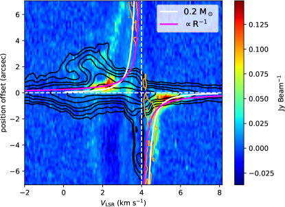
Figure 16: ALMA Cycle 4 SO ($\nu=0,J=8_{8}-7_{7}$, black contours), ALMA Cycle 2 C¹⁸O with natural weighting (J = 2-1, color), and DCO+ (J = 3-2, orange) position velocity (PV) diagram on VLA1623B. The contours are in steps of 5 $\sigma$, 10 $\sigma$, 20 $\sigma$, 30 $\sigma$, 50 $\sigma$, 70 $\sigma$, 90 $\sigma$, where $\sigma=$ 15, 8 mJy beam^-1 for SO and DCO+ respectively. The magenta solid line is the infall profile with conserved angular momentum, and white solid line is the Keplerian rotation profile with central stellar mass of 0.2 $M_{\odot}$ with an inclination angle of $55^{\circ}$. Note that the central velocity of SO is shifted to 3 kms^-1.

After identifying the corresponding SO streams around VLA1623A circumbinary disk by comparing with the C¹⁸O data, PV diagrams are used to further study their interactions. We plot the PV diagrams of SO ($J=8_{8}-7_{7}$), C¹⁸O (J = 2-1), and DCO⁺ (J = 3-2) across VLA1623A circumbinary disk in Figure 15. The PV cut is aligned along the red line shown in Figure 2. The black SO contours marked out the extended high velocity SO emission on the blue-shifted side. It spreads out from -4$\farcs$0 $\sim$ 2$\farcs$0 with the center of the circumbinary disk positioned at 0$\farcs$0. The spatially extended high velocity SO on the blue-shifted side suggests there are mild accretion shocks, which are likely produced by the interaction between the accretion flow I, III and the circumbinary disk. Since the northern SO stream is perpendicular to the outflow direction, the contribution from interaction with an outflow is ruled out. In contrast, the SO on the red-shifted part is very spatially compact and locates only in the center of the circumbinary disk. The compact structure of the red-shifted SO suggests that there is no violent accretion shocks between the red-shifted accretion flow VI and the circumbinary disk around VLA1623A.

Figure 17: VLA1623A and blue-shifted structure I, II, III and VIII channel maps. The color represents the C¹⁸O J = 2-1 (Briggs -1.5) emission identified by the dendrogram algorithm. The magenta contours are 0.88 mm continuum data. The contours are in step of 5 $\sigma$, where $\sigma=5\times 10^{-4}$ Jy beam^-1.

3.9 Outflow signatures from VLA1623A and VLA1623B

In Figure 17 we plot the channel maps of the four large scale blue-shifted structures from the dendrogram analysis. In previous sections, based on the CO outflows and SO shocks in Figure 13, we have established that structure II is an outflow cavity wall. At the exact same position as structure II in Figure 17, we discovered a similar elongated structure (VIII) at lower velocity ($2.953\sim 3.293\,km\,s^{-1}$). Structure (VIII) has the same shape and position as structure II, and it is also on top of both the CO outflow and SO shocked southern stream suggesting it is also an outflow cavity wall. The two outflows cavity walls traveling at different velocities is a strong evidence indicating that there are two outflows in the plane of sky, coming from VLA1623A and VLA1623B, respectively. Cycle 0 CO results (Santangelo et al., 2015), which is almost completely filtered out by ALMA, suggests that VLA1623B is driving a much more compact outflow, and the authors associate the slower large-scale outflows with VLA1623A.

In contrast, our high resolution Cycle 6 CO data and the discovery of outflow cavity walls (Structure II and VIII) suggests otherwise. There are two outflows overlaying on top of each other in the plane of sky. The large scale outflows come from both VLA1623A and VLA1623B as shown by the two outflow cavity walls at two different velocities. From our Cycle 6 CO data we found the outflow from VLA1623B is more red-shifted compared to VLA1623A, therefore we associate the outflow cavity II with outflows from VLA1623A and outflow cavity VIII with outflows from VLA1623B. Multi-tracer analysis to distinguish between the two outflows would be presented in a future paper.

3.10 Existence of Wall-like structure south of VLA1623B

The PV diagrams of SO ($J=8_{8}-7_{7}$), C¹⁸O (J = 2-1), and DCO⁺ (J = 3-2) on VLA1623B, centered at $\alpha$(J2000) = 16^h26^m26$\fs$305, $\delta$(J2000) = –24°24′30$\farcs$705 with position angle of 222.8^∘ are plotted in Figure 16. In the blue-shifted region at the position offset around 3$\farcs$0, we observed the similar extended high velocity blue-shifted SO feature (compare to Figure 15), which corresponds to the shock fronts of the accretion flow I and III. The SO emission has a very wide line width ($>$10 kms^-1) at the position offset between $\pm$1$\farcs$0 (across VLA1623B). The huge velocity dispersion on VLA1623B indicates there is a huge change in velocity on VLA1623B and huge shock fronts are formed. Furthermore, at the south of VLA1623B the materials only have velocity around 4.0 kms^-1 suggesting the SO is at rest. The huge change in SO velocity and materials (C¹⁸O, SO, DCO⁺) on the south of the VLA1623B are at rest both suggests a wall-like structure is located south of VLA1623B.

In the previous section, the red-shifted accretion flow VI is identified to be connecting to VLA1623B (See Figure 6,  Figure 8). When the materials from the blue-shifted accretion flow III accrete onto VLA1623B, they are quickly stopped by the red-shifted accretion flow VI (shown in Figure 8). The collision between blue-shifted accretion flow III and red-shifted accretion flow VI on VLA1623B slows down the materials and forms an extended wall-like structure south of VLA1623B. This explains why no violent accretion shocks from the red-shifted accretion flow VI is observed around VLA1623A circumbinary disk. The red-shifted accretion flow VI is already significantly slowed down around VLA1623B.

To constrain the size of the wall-like structure south of VLA1623B, we analyze the SO PV diagram in Figure 16. In Figure 16, around the systematic velocity 4 kms^-1 there exists a long extended SO and DCO⁺ on the south (negative offset) side of VLA1623B. DCO⁺ would have abundance enhancement when the temperature is below CO freeze-out temperature (Mathews et al., 2013). However, DCO⁺ emission at rest around the disk is contaminated from the envelope making it not ideal to trace the wall-like structure south of the circumbinary disk. On the other hand, SO which has high sublimation temperature of 50K traces the shocks region near the centrifugal barrier (Sakai et al., 2014). The SO in Figure 16 extends to around 6$\farcs$5 ($\sim$ 780 AU). Therefore, the wall on the south side of VLA1623B has a plane of sky width at least 780 AU.

4 Discussions

4.1 Explanations of the super-Keplerian rotation in the inner region of the disk

Figure 18: (a). Position-Velocity (PV) cut of C¹⁸O J = 2-1 ALMA Cycle 2 VLA1623A Keplerian disk (natural weighting), centered at VLA1623A with position angle 209.82^∘. The white and magenta solid lines represent the Keplerian rotation profile with a central mass of 0.2 $M_{\odot}$ and 0.5 $M_{\odot}$ respectively. The inclination angle is set to be $55^{\circ}$. The dotted lines marked their corresponding escape velocity. The white arrow marks the position of the Keplerian disk that is asymmetric in motion. The red arrow marks the blue-shifted accretion flow I. The vertical black lines mark the velocities of the major large scale emission. (b). The zoomed in image of (a).

As discussed in § 3.2, we identified a blue-shifted (super-Keplerian) rotation region between 1.5  kms^-1 and 2.0  kms^-1 within 1$\farcs$0 in position offset. A clear gap between VLA1623A circumbinary disk and the blue-shifted accretion flow I can be found between 2.3 km s^-1 to 3.2 km s^-1 in Figure 7 as well as the PV diagram in Figure 4 a. marked by a white arrow. This gap sets a clear boundary between blue-shifted accretion flow I and the disk. This further rules out the possibility that the blue-shifted super-Keplerian rotation region is part of any large scale structures or accretion flows in the line of sight as the disk and accretion flow I are clearly separate in position and velocity space by a gap is shown in Figure 4 a. The fact that magenta infall velocity profile passes through the inner region of the disk, but deviates significantly on the outer edge of the circumbinary disk on the red-shift side suggests this high-velocity super-Keplerian region inside the disk has different angular momentum from the large scale accretion flows. Thus, an important question remained to be answered is whether or not the high-velocity blue-shifted component (super-Keplerian rotation region) is part of the disk structure?

One possible explanation for this super-Keplerian rotation region is disk flaring. For a flared disk, due to the z-direction projection effect it is possible the inner region of the disk is projected to positions further away from the disk center. To take into account of disk flaring and projection effects, we developed a more sophisticated 3D flared disk model to model the observation data. By comparing the model with the ALMA data, we tested this interpretation.

As shown in Figure 20, all the flared disk models (thick black contours) can’t explain the blue-shifted super-Keplerian rotation region in 0$\farcs$5 position offset at velocity range 1.5 $\sim$ 2.0 kms^-1. The mismatch between the flared disk model and the data shows that the super-Keplerian rotation region is not due to projection effects of a flared disk. If the super-Keplerian region is due to projection effects, one would expect the disk to be very flared, so the higher velocity materials in the inner region can be projected at larger position offsets. In Figure 9 at 1.5 km s^-1 the white Keplerian rotation line has a position offset of 0$\farcs$2 ($\sim$ 24 AU) lower than the C¹⁸O data which locates at 0$\farcs$5 $\sim$ 0$\farcs$7 (60 $\sim$ 80 AU). Considering an inclination of 55^∘, if the super-Keplerian rotation region is due to project effects, then one would expect the majority of the C¹⁸O is distributed around 40$\sim$70 AU above the disk plane. To achieve this, the scale height of the disk, location where density drops to a fraction of 1/e from the mid-plane, must be much greater than 40 AU. Our flared disk models constrained the disk scale height to be within 15 AU, and thus shows this super-Keplerian rotation region is not due to projection effects from a flared disk.

The flat and flared Keplerian disk modeling cannot explain the high-velocity super-Keplerian rotation region in the inner part of the disk. Previous dendrogram analyses found a gap between accretion flows and circumbinary disk suggesting that this super-Keplerian rotation region is not coming from large scale accretion flows in the line of sight. It is within the 180  AU of the circumbinary disk. There are two possible explanations to this super-Keplerian rotation region: (i) It is due to collision with infalling materials from the envelope. The materials from above the circumbinary disk plane fall onto the inner region of the circumbinary disk. The collision resulted in the net gain of angular momentum in the inner region of the disk. (ii) Previous Cycle 0 data underestimate the mass, the combined mass of the binary should be 0.3$\sim$0.5 $M_{\odot}$ instead of 0.2 $M_{\odot}$.

The collision between the circumbinary disk and the infalling materials from above the disk plane can provide enough acceleration to explain the super-Keplerian rotation region. Previously, we have used the dendrogram to identify large scale accretion flows. We found a 120 AU wide gap between the accretion flow I and the circumbinary disk. In order to create high-velocity C¹⁸O component only in the inner region of the circumbinary disk, the infalling materials can only collide with the circumbinary disk from above the disk plane. Moreover, with outflows perpendicular to the disk the allowed infalling angles lie only between the outflow and the disk. Note that one important feature of the super-Keplerian region is that it is symmetric in both blue and red-shifted region. Consider the materials moving in a 60 AU circular orbit with circular velocity on the order of $\sim 2$ kms^-1, the time scale to complete 1 orbit is on the order of $\sim$200 years. This time scale is significantly smaller than the disk evolution time scales. We expect any asymmetry features caused by the infalling materials onto the disk to be smoothed out, creating a symmetric feature on both blue and red-shifted side of the PV diagram. The short orbital period compared to the outer disk evolution timescales ($\sim 10^{4}$ years) also implies any infalling signatures are only transient structures making them unlikely to be observed if the infalling materials are not continuously supplied by the envelope.

Another possible explanation of the inner super-Keplerian region is a higher combined binary mass. This would mean the previous mass estimate (0.2 $M_{\odot}$) from Cycle 0 (Murillo et al., 2013) underestimates the mass. To check this possibility, we plot the escape velocities as dotted lines for both combined binary mass of 0.2 $M_{\odot}$ and 0.5 $M_{\odot}$ in Figure 18.

The upper left stream (Blue-shifted accretion flow I marked by the red arrow) appears to match the escape velocity for 0.5 $M_{\odot}$. Infalling streams must have velocity less than the escape velocity. Thus, the sum of surrounding envelope mass and combined binary mass must be greater than 0.5 $M_{\odot}$. Since Class 0 protostar is still deeply embedded in the envelope (Seifried et al., 2015), and envelope mass could be comparable or larger than the central star, the motion of accretion flows cannot completely break the degeneracy in combined binary mass.

Figure 19: Cartoon diagram of accretion flows and disk interactions studied in this work towards VLA1623A circumbinary disk and VLA1623B for combined VLA1623A binary mass 0.5 M_⊙.

Unlike the case with the combined binary mass of 0.2 $M_{\odot}$ (Murillo et al., 2013) (white solid line Figure 18), the Keplerian rotation line for combined binary mass of 0.5 $M_{\odot}$ (magenta solid line Figure 18) passes through the high velocity blue-shifted component perfectly. It will however need the circumbinary disk to be asymmetric in the outer region. For the magenta solid lines, the blue-shifted disk between 1$\farcs$0 to 2$\farcs$0 rotates faster than the Keplerian rotation, while at the same position the red-shifted disk is sub-Keplerian (marked by white arrows). The observation of blue-shifted SO shocks north of the disk might be a possible explanation of this asymmetry in motion.

To break the mass degeneracy, we fit the PV diagram across VLA1623A with a careful treatment. First, we masked out all pixels with negative flux. Then for each velocity channel we search for the peaks above 3 sigma at different position. This will allow us to identify different structures at each velocity channels. Then we remove the infalling stream (red arrow in Figure 18) and uses the data that are at least 0.5 kms^-1 away from the systematic velocity (4.0 kms^-1) to prevent contamination. Intensity weighted position average is then calculated to determine the representative disk position for each velocity channel. The non-linear least squares fitting result yields a central binary mass of $0.3$ M_⊙. If one assumes that all gas should be sub-Keplerian in the disk and the Keplerian rotation line should “match only the edge of the PV diagram”, then a mass of $0.5$ M_⊙ would be obtained.

From the flat and flared disk modeling to the infalling streams from accretion flow I, we have concluded that the most plausible explanation of super-Keplerian motion is the underestimation of combined binary mass in VLA1623A. The combined binary mass from VLA1623A should be 0.3$\sim$ 0.5 $M_{\odot}$.

4.2 Summarized Picture

The results of flat and flared disk modeling show that VLA1623A circumbinary disk is a large flat Keplerian disk with a size of 180 AU and a combined binary mass of 0.3$\sim$ 0.5 $M_{\odot}$. At the edge of the circumbinary disk, it is estimated to have a thickness around 30 AU based on the of CMU modeling, which shows the thickness of the incoming accretion flows at the centrifugal radius is around 30 AU (Cheong et al. 2019; submitted).

In the previous sections, we used both SO $J=8_{8}-7_{7}$ and C¹⁸O J = 2-1 data to study how the accretion flows interact with the circumbinary disk around VLA1623A and VLA1623B. A cartoon diagram of their interactions is summarized in Figure 19 for combined binary mass 0.5 M_⊙. In short, there are around 3 main accretion flows found in this study: blue-shifted accretion flow I, III, and red-shifted accretion flow VI as summarized in Table 3.

Table 3: Accretion flows around VLA1623A

Structure	Velocity	SO data	C18O data
	(kms-1)
Accretion	2.02 $\sim$ 3.60	Figure 11 East	Figure 7
flows I		SO stream
Outflow		Figure 11	Figure 12 b
cavity wall	1.27 $\sim$ 2.21	South SO	South C18O
II		stream	stream
Accretion		Figure 11	Figure 12 b
flows III	1.27 $\sim$ 2.21	North SO	North C18O
		stream	stream
Accretion		Figure 11	Figure 8, 12 a
flows VI	3.45 $\sim$ 4.79	West SO	West
		stream	C18O clump
Outflow		Figure 14
cavity wall	2.95 $\sim$ 3.29	channel	Figure 17
VIII		3.084 km s-1

From the extended emission in the SO PV diagram (Figure 15), we identified an accretion shock north of the circumbinary disk around VLA1623A. This SO accretion shocks are produced by the blue-shifted accretion flows I and III colliding with the edge of the circumbinary disk. The blue-shifted accretion flow III also collide with the red-shifted accretion flows VI on VLA1623B (Figure 16). The collision creates extremely wide SO line width ($>$ 10 kms^-1) corresponding to the violent shocks on VLA1623B. The collision significantly slows down and stop the materials from the red-shifted accretion flows VI at a position south of the VLA1623B forming a wall-like structure as shown in Figure 16.

The materials from red-shifted accretion flow VI continue to pile up, spread to the south of VLA1623A circumbinary disk and infall towards it. The infall of rotating materials are connected to the boundary of the disk and extended up to $\sim$ 500 AU south of the circumbinary disk. This explains the extended red-shifted C¹⁸O emission in Figure 3. Furthermore, the outflow collides with this infall rotating materials and forms a long extended SO South stream in Figure 13 with a peak located around 4$\farcs$0 south from the disk. The overall picture of the interactions between accretion flows and circumbinary disk around VLA1623A and VLA1623B is summarized in Figure 19.

4.3 SO North of the VLA 1623A circumbinary disk and VLA 1623B; shocks or infall/rotation?

The SO north of the disk and VLA1623B in Figure 15 and Figure 16 (more positive positional offsets) appears to have similar linewidth as compared to C¹⁸O which traces infall and rotation. However, SO north of the VLA1623A circumbinary disk and VLA1623B is actually tracing a mild shock instead of infall and rotation. In the higher 0$\farcs$3 resolution SO 3 $\Sigma$  $\nu=0$  7(8)-6(7) observation (Project code: 2018.1.00388.S, PI: Cheng-Han Hsieh), 2 compact SO peaks are observed north of VLA1623A and VLA1623B (Hsieh et al. 2019 in prep). The SO linewidths of those peaks are 4 kms^-1 and 7 kms^-1 which are significantly larger than the C¹⁸O linewidth (Hsieh et al. 2019 in prep) suggesting they are very likely originated from a shock. More in-depth study of shocks around VLA1623 system would be present in the future paper.

5 Conclusions

This work presents a detailed analysis of VLA1623A circumbinary disk and VLA1623B. The results can be summarized as the following:

1. The super-Keplerian rotation region inside the VLA1623A circumbinary disk cannot be fitted properly with either Flat or Flared Keplerian disk models with binary mass 0.2 M_⊙. This is due to the results from Cycle 0 data significantly underestimate the binary mass. Based on accretion streams (Figure 18) and disk modeling, we suggest the combined binary mass for VLA1623A should be $0.3\sim$0.5 M_⊙.

2. From the SO PV diagrams, we detect the existence of a wall-like structure south of VLA1623B. The wall has a plane of sky width of around 780 AU on the VLA1623B side. Furthermore, plausible pictures of how accretion flows interact with VLA1623A circumbinary disk and VLA1623B are constructed and shown in Figure 19.

3. From the dendrogram analysis, we discovered two outflow cavity walls (structure II and VIII) at the same position moving at different velocities. This is strong evidence suggesting that there are two large-scale CO outflows in the plane of sky on top of each other originated from VLA1623A and VLA1623B.

Appendix A Estimation of Centrifugal Radius

Consider a simple disk such that the gravitational acceleration balances the centrifugal force where $j$ is the specific angular momentum.

$$\frac{GM_{*}}{r^{2}}={\frac{j^{2}}{r^{3}}}$$ (A1)

The centrifugal radius $r_{c}$ can be expressed in terms of the specific angular momentum ($j$) as following,

$$r_{c}={\frac{j^{2}}{G{M_{*}}}}$$ (A2)

If the disk is in hydro-static equilibrium in the vertical direction (z), the total column density ($\sigma$) can be expressed in terms of the volume density at mid-plane ($\rho_{c}$) as following:

$$\sigma=\sqrt[]{\frac{2c_{s}^{2}\rho_{c}}{\pi G}}$$ (A3)

where $c_{s}$ is the sound speed. It is simple to show that

$$\frac{c_{s}j}{G{M_{*}}}=\frac{c_{s}\omega_{c}r^{2}}{G\sigma\pi r^{2}}=\frac{\omega_{c}}{\sqrt[]{2\pi G\rho_{c}}}$$ (A4)

Numerical simulations by Matsumoto et al. (1997) has shown the factor

$$\frac{\omega_{c}}{\sqrt[]{2\pi G\rho_{c}}}\approx 0.3.$$ (A5)

Therefore, the centrifugal radius can be expressed as:

$$r_{c}={\frac{j^{2}}{G{M_{*}}}}=\frac{GM_{*}}{c_{s}^{2}}\Big{(}\frac{c_{s}j}{G{M_{*}}}\Big{)}^{2}\approx 0.09\frac{G{M_{*}}}{c_{s}^{2}}.$$ (A6)

Using the sound speed relation,

$$c_{s}^{2}=\frac{k_{B}T}{\mu m_{p},}$$ (A7)

where $\mu\approx 2.3$ and consider a typical disk temperature of 30 K and a combined binary mass of 0.2 $M_{\odot}$, we found that the sound speed $c_{s}\approx$ 0.33 km s^-1 and the corresponding centrifugal radius is $\sim$ 148 AU. For simplicity, the centrifugal radius is close to $\sim$ 120 AU, so we set the crossover point of constant angular momentum with the keplerian curve to be at 1$\farcs$0 in position offset, which corresponds to a specific angular momentum of 120 AU km s^-1.

Appendix B Flared Disk Modeling Results

Figure 20 displays the results of the flared disk modeling without zoomed in on the red-shifted components.

Figure 20: Position-Velocity (PV) diagrams of VLA1623A keplerian disk overlaid with flared disk model contours with different vertical scale height $h_{0}$ and density power-law $a$. The color represents the PV diagram of C¹⁸O J = 2-1 emission centered at VLA1623A and the thin black contours are plotted for 3 $\sigma$, 5 $\sigma$, 7 $\sigma$, 9 $\sigma$, 11 $\sigma$, 13 $\sigma$, 15 $\sigma$ with $\sigma=9$ mJybeam^-1. The thick black contours are from the Flared Keplerian disk model with central binary mass 0.2 $M_{\odot}$. The contours are in steps of 0.2, 0.4, 0.6, 0.8, 0.95 of the maximum flux in the model. The brown contour marks the 7 $\sigma$ line used for model comparison. The white and gray solid lines represent the Keplerian rotation curve with central star mass 0.2 and 0.5 $M_{\odot}$ and an inclination angle of $55^{\circ}$. The magenta line represents the infall velocity profile with conserved angular momentum. The vertical white lines mark the velocity of the major large scale emission.

References

- Andre et al. (1990) Andre, P., Martin-Pintado, J., Despois, D., et al. 1990, A&A, 236, 180.
- Artymowicz, & Lubow (1994) Artymowicz, P., & Lubow, S. H. 1994, ApJ, 421, 651.
- Andre et al. (1993) Andre, P., Ward-Thompson, D., & Barsony, M. 1993, ApJ, 406, 122.
- Aso et al. (2017) Aso, Y., Ohashi, N., Aikawa, Y., et al. 2017, ApJ, 849, 56
- Beaumont et al. (2014) Beaumont, C., Robitaille, T., & Borkin, M. 2014, Glue: Linked data visualizations across multiple files, ascl:1402.002.
- Boss, & Keiser (2014) Boss, A. P., & Keiser, S. A. 2014, ApJ, 794, 44.
- Burkert, & Bodenheimer (1993) Burkert, A., & Bodenheimer, P. 1993, MNRAS, 264, 798.
- Cassen, & Moosman (1981) Cassen, P., & Moosman, A. 1981, Icarus, 48, 353.
- Chiang, & Goldreich (1997) Chiang, E. I., & Goldreich, P. 1997, ApJ, 490, 368.
- Chou et al. (2014) Chou, T.-L., Takakuwa, S., Yen, H.-W., et al. 2014, ApJ, 796, 70.
- Chen et al. (2013) Chen, X., Arce, H. G., Zhang, Q., et al. 2013, ApJ, 768, 110
- Connelley et al. (2008) Connelley, M. S., Reipurth, B., & Tokunaga, A. T. 2008, AJ, 135, 2526.
- Lee et al. (2017) Lee, C.-F., Li, Z.-Y., Ho, P. T. P., et al. 2017, ApJ, 843, 27.
- Davidson et al. (2011) Davidson, J. A., Novak, G., Matthews, T. G., et al. 2011, ApJ, 732, 97.
- Dent et al. (1995) Dent, W. R. F., Matthews, H. E., & Walther, D. M. 1995, MNRAS, 277, 193.
- Duchêne et al. (2007) Duchêne, G., Bontemps, S., Bouvier, J., et al. 2007, A&A, 476, 229.
- Dullemond et al. (2012) Dullemond, C. P., Juhasz, A., Pohl, A., et al. 2012, Astrophysics Source Code Library , ascl:1202.015.
- Dutrey et al. (2014) Dutrey, A., di Folco, E., Guilloteau, S., et al. 2014, Nature, 514, 600.
- Dutrey et al. (2016) Dutrey, A., Di Folco, E., Beck, T., et al. 2016, Astronomy and Astrophysics Review, 24, 5.
- Fromang, & Stone (2009) Fromang, S., & Stone, J. M. 2009, A&A, 507, 19.
- Guan, & Gammie (2009) Guan, X., & Gammie, C. F. 2009, ApJ, 697, 1901.
- Guilloteau, & Dutrey (1998) Guilloteau, S., & Dutrey, A. 1998, A&A, 339, 467.
- Guilloteau et al. (2011) Guilloteau, S., Dutrey, A., Piétu, V., et al. 2011, A&A, 529, A105.
- Harris et al. (2018) Harris, R. J., Cox, E. G., Looney, L. W., et al. 2018, ApJ, 861, 91.
- Hennebelle, & Ciardi (2009) Hennebelle, P., & Ciardi, A. 2009, A&A, 506, L29.
- Hennebelle et al. (2016) Hennebelle, P., Commerçon, B., Chabrier, G., et al. 2016, ApJ, 830, L8.
- Hull et al. (2013) Hull, C. L. H., Plambeck, R. L., Bolatto, A. D., et al. 2013, ApJ, 768, 159.
- Hull et al. (2014) Hull, C. L. H., Plambeck, R. L., Kwon, W., et al. 2014, The Astrophysical Journal Supplement Series, 213, 13.
- Inutsuka, & Miyama (1992) Inutsuka, S.-I., & Miyama, S. M. 1992, ApJ, 388, 392.
- Jørgensen et al. (2009) Jørgensen, J. K., van Dishoeck, E. F., Visser, R., et al. 2009, A&A, 507, 861.
- Lesur, & Longaretti (2009) Lesur, G., & Longaretti, P.-Y. 2009, A&A, 504, 309.
- Lizano et al. (2016) Lizano, S., Tapia, C., Boehler, Y., et al. 2016, ApJ, 817, 35.
- Loinard et al. (2008) Loinard, L., Torres, R. M., Mioduszewski, A. J., et al. 2008, ApJ, 675, L29.
- Lubow (1991) Lubow, S. H. 1991, ApJ, 381, 259.
- Mathews et al. (2013) Mathews, G. S., Klaassen, P. D., Juhász, A., et al. 2013, A&A, 557, A132.
- Matsumoto et al. (1997) Matsumoto, T., Hanawa, T., & Nakamura, F. 1997, ApJ, 478, 569
- Mayama et al. (2010) Mayama, S., Tamura, M., Hanawa, T., et al. 2010, Science, 327, 306.
- Mellon, & Li (2008) Mellon, R. R., & Li, Z.-Y. 2008, ApJ, 681, 1356.
- Murillo et al. (2013) Murillo, N. M., Lai, S.-P., Bruderer, S., et al. 2013, A&A, 560, A103.
- Murillo, & Lai (2013) Murillo, N. M., & Lai, S.-P. 2013, ApJ, 764, L15.
- Murillo et al. (2018) Murillo, N. M., van Dishoeck, E. F., van der Wiel, M. H. D., et al. 2018, ArXiv e-prints , arXiv:1805.05205.
- Offner et al. (2010) Offner, S. S. R., Kratter, K. M., Matzner, C. D., et al. 2010, ApJ, 725, 1485.
- Ortiz-León et al. (2017) Ortiz-León, G. N., Loinard, L., Kounkel, M. A., et al. 2017, ApJ, 834, 141.
- Padoan, & Nordlund (2002) Padoan, P., & Nordlund, Å. 2002, ApJ, 576, 870.
- Pineda et al. (2015) Pineda, J. E., Offner, S. S. R., Parker, R. J., et al. 2015, Nature, 518, 213.
- Raghavan et al. (2010) Raghavan, D., McAlister, H. A., Henry, T. J., et al. 2010, The Astrophysical Journal Supplement Series, 190, 1.
- Sakai et al. (2014) Sakai, N., Sakai, T., Hirota, T., et al. 2014, Nature, 507, 78.
- Santangelo et al. (2015) Santangelo, G., Murillo, N. M., Nisini, B., et al. 2015, A&A, 581, A91.
- Sana, & Evans (2011) Sana, H., & Evans, C. J. 2011, Active OB Stars: Structure, Evolution, Mass Loss, and Critical Limits, 474.
- Santos-Lima et al. (2012) Santos-Lima, R., de Gouveia Dal Pino, E. M., & Lazarian, A. 2012, ApJ, 747, 21
- Santos-Lima et al. (2013) Santos-Lima, R., de Gouveia Dal Pino, E. M., & Lazarian, A. 2013, MNRAS, 429, 3371
- Schekochihin et al. (2004) Schekochihin, A. A., Cowley, S. C., Maron, J. L., et al. 2004, Phys. Rev. Lett., 92, 54502.
- Seifried et al. (2015) Seifried, D., Banerjee, R., Pudritz, R. E., et al. 2015, MNRAS, 446, 2776.
- Shu et al. (1987) Shu, F. H., Adams, F. C., & Lizano, S. 1987, Annual Review of Astronomy and Astrophysics, 25, 23.
- Shu et al. (2007) Shu, F. H., Galli, D., Lizano, S., et al. 2007, ApJ, 665, 535.
- Takakuwa et al. (2012) Takakuwa, S., Saito, M., Lim, J., et al. 2012, ApJ, 754, 52.
- Takakuwa et al. (2017) Takakuwa, S., Saigo, K., Matsumoto, T., et al. 2017, ApJ, 837, 86.
- Tobin et al. (2013) Tobin, J. J., Hartmann, L., Chiang, H.-F., et al. 2013, ApJ, 771, 48.
- Tobin et al. (2016) Tobin, J. J., Looney, L. W., Li, Z.-Y., et al. 2016, ApJ, 818, 73
- Tobin et al. (2018) Tobin, J. J., Bos, S. P., Dunham, M. M., et al. 2018, ApJ, 856, 164.
- Tomida et al. (2015) Tomida, K., Okuzumi, S., & Machida, M. N. 2015, ApJ, 801, 117.
- Tang et al. (2014) Tang, Y.-W., Dutrey, A., Guilloteau, S., et al. 2014, ApJ, 793, 10.
- Tang et al. (2016) Tang, Y.-W., Dutrey, A., Guilloteau, S., et al. 2016, ApJ, 820, 19.
- Ulrich (1976) Ulrich, R. K. 1976, ApJ, 210, 377.
- Yen et al. (2013) Yen, H.-W., Takakuwa, S., Ohashi, N., et al. 2013, ApJ, 772, 22.
- Yen et al. (2014) Yen, H.-W., Takakuwa, S., Ohashi, N., et al. 2014, ApJ, 793, 1.
- Yu & Chernin (1997) Yu, T., & Chernin, L. M. 1997, ApJ, 479, L63.