Parametric identification of the dynamics
of inter-sectoral balance: modelling and forecasting

Abstract

This work is devoted to modelling and identification of the dynamics of the inter-sectoral balance of a macroeconomic system. An approach to the problem of specification and identification of a weakly formalized dynamical system is developed. A matching procedure for parameters of a linear stationary Cauchy problem with a decomposition of its upshot trend and a periodic component, is proposed. Moreover, an approach for detection of significant harmonic waves, which are inherent to real macroeconomic dynamical systems, is developed.

Keywords: Leontief’s model, cyclical processes, harmonic waves, prediction.

2010 Mathematics Subject Classification: 91B02, 91B84.

1 Introduction

For any dynamical object (technical, economic, environmental, etc.), the most critical is the problem of limited resources and their optimal use. Thereby, there is a need to build mathematical models that adequately describe the existing trends and provide high-precision predictive properties of the dynamical systems. Therefore, it is necessary to evaluate the quality of mathematical models of dynamical processes through the prism of imitation and predictive properties.

The meaning of mathematical modelling, as a research method, is determined by the fact that a model is a conceptual tool focused on the analysis and forecasting of dynamical processes using differential or differential-algebraic equations. However, the parameters of these equations are usually unknown in advance. Therefore, in practice, any direct problem (imitation, prediction, and optimization) is always preceded by an inverse problem (model specification and identification of parameters and variables included in it).

To construct dynamical models in economics, it is necessary to formulate principles, based on economic theory, and consider equations that adequately determine the evolution of the investigated process. The functioning of a market economy, as well as any economic system, is not uniform and uninterrupted. An important tool for its prediction is the dynamical model of inter-industry equilibrium balance developed by Leontief (the so called “Leontief’s input-output model”), which became the basis of mathematical economics [Leontief] . Leontief’s input-output model is described by a system of linear differential equations in which the input is the non-productive consumption of sectors, and the output is the issue of these sectors. In practice, the matrices of the system of differential equations are unknown in advance. Therefore, there is a need to evaluate them based on statistical information of the macroeconomic system under study, for a certain period of time. The problem of parametric identification of macroeconomic dynamics is discussed in the papers [Ramsay] ; [NazarenkoFil] ; Olena01 ; Olena02 .

One feature of the dynamical Leontief model is that it can be considered as taking into account the cyclical nature of the macroeconomic processes, typical for developed countries of Western Europe, USA, Canada, Japan, and others [Diebolt] ; [Korotaev] . According to statistical analysis, their economic growth (upturn phase) alternates with the processes of stagnation and decline in production volumes (downturn phase), i.e., a decline in all the economic activity. After a decline phase, again, the economic cycle continues, similarly with ups and downs. Such periodic fluctuations indicate a cyclical nature of the economic development.

The analysis of the input-output model is critical for developing government regulatory programs, that are an integral part of the economic and environmental policy for any developed market system. Such an analysis is a useful tool for studying the strategic directions of economic development, the expansion of dynamical inter-industry relations, and the interaction between economic sectors and the natural environment [Fied] ; [Dobos] .

This paper is organized as follows. Section 2 is devoted to a detailed economic and mathematical description of the Leontief macroeconomic model. Section 3 focuses on the problem of specification and identification of this model and Section 4 to the testing of the Leontief model with time series data of a real macroeconomic dynamics. In Section 5, the main conclusions are carried out.

2 Problem statement

The static model of inter-industry balance is obtained when one equates the net production of branches to the final demand for the products of these industries:

$$\textbf{x}-A\textbf{x}=\textbf{y}\;,$$ (1)

where ${\bf x}=(x_{1},x_{2},\ldots,x_{n})^{{}^{\prime}}$ is the column vector of gross output by industries; ${\bf y}=(y_{1},y_{2},\ldots,y_{n})^{{}^{\prime}}$ is the column vector of final demand; and $A$ is the matrix of direct costs. The vector of final demand ${\bf y}$ can be represented as a sum of two vectors: investments, ${\bf y}_{1}(t)=B\dot{\bf x}(t)$, and consumer products, ${\bf y}_{2}(t)={\bf u}(t)$. Then, the model of dynamical inter-industry balance is

$${\bf x}(t)=A{\bf x}(t)+B\dot{\bf x}(t)+{\bf u}(t)\;,\ \ \dot{\bf x}(t)=\frac{d{\bf x}(t)}{dt}\;,$$ (2)

where ${\bf u}(t)$ is the vector-column of final (non-productive) consumption and $B$ is the matrix of capital coefficients. A discrete-time dynamic balance model can be reduced to a model with continuous time as follows:

$$B\dot{\bf x}(t)=(E-A){\bf x}(t)-{\bf u}(t)\;.$$ (3)

If the inverse matrix $B^{-1}$ exists, then the Leontief’s model can be rewritten as a linear multiply-connected system, with the final consumption vector ${\bf u}(t)$ as the input and with the gross output vector ${\bf x}(t)$ as the output:

$$\dot{\bf x}(t)=B^{-1}(E-A){\bf x}(t)-B^{-1}{\bf u}(t)\;,\ \ t\in[t_{0},t_{f}]\;.$$ (4)

The differential equation (4) must be supplemented with the boundary condition

$${\bf x}(t_{*})={\bf x}_{*}\;,$$ (5)

where $t_{*}$ is the point of the segment $[t_{0},t_{f}]$ at which the boundary state is specified. To determine the unknown parameters $A$, $B$, and ${\bf x}_{*}$ of the Cauchy problem (4)–(5), in accordance with the methodology proposed in [Nazarenko] , we divide the interval $[t_{0},t_{f}]$ into two intervals: the identification period $[t_{0},t_{*})$ and the forecasting period $[t_{*},t_{f}]$. We assume that the base period $[t_{0},t_{*})$ has statistical information ${\bf x}_{t}$ and ${\bf y}_{t}$ regarding industry’s outputs and consumption at its discrete-times $t=1,2,\ldots,N$, and the model will be adjusted for the vector of unknown coefficients ${\bf\theta}$. For the interval $[t_{*},t_{f}]$, we assume that $t_{f}-t_{*}\ll N$. Through this approach, the boundary condition (5) is satisfied in the first integer point of the forecast period. Then, if the model is stationary, and due to the inertia of the dynamical system, the vector ${\bf\theta}$ can be translated for the forecast period. The stationariness of the model is characterized by the high quality of approximation and forecasting and robustness [Green] . However, for modelling and prediction of linear stationary models, the identification period $N$ should be large enough to stabilize the interrelations between the elements of the system.

3 Algorithm

First of all, for convenience, we make the data dimensionless and then, we proceed by solving the Cauchy problem (4)–(5). To do this, we need to specify the vector of phase coordinates ${\bf x}(t)$ and estimate the unknown parameters that will appear in the specification process [Nazarenko] . The vector ${\bf x}(t)$ is searched by decomposing the trajectories of the phase coordinates motion into components [Nazarenko] . If these trajectories are defined, then the vector ${\bf u}(t)$ can be found. It will be supplied to the input of the dynamical system and it can be used to solve the problem of specifying the sectors’ output and manage their movement. The vector ${\bf u}$ will be considered as a control vector and it can be found using the inverse relationship

$${\bf u}(t)=P{\bf x}(t)-B\dot{\bf x}(t)\;,\ \ P=E-A\;.$$ (6)

At each time step, the vector $\bf{u}$ is a function of the phase coordinates and their derivatives. The regulator implements the critical idea of control theory: the principle of inverse connection, being used for identifying the model (6). In our research, the regulator consists of two devices. At any time $t$, they form a total value of phase coordinates (issues sectors) and controls (non-productive consumption sectors):

$${\bf x}(t)=\sum\limits_{m=1}^{n}{\bf x}_{m}(t)\;,\ \ {\bf u}(t)=\sum\limits_{m=1}^{n}{\bf u}_{m}(t)\;.$$ (7)

If the modelling trajectories ${\bf x}(t)$ and ${\bf u}(t)$, where ${\bf x}(t)=(x_{1}(t),x_{2}(t),\ldots,x_{n}(t))^{{}^{\prime}}$ and ${\bf u}(t)=(u_{1}(t),u_{2}(t),\ldots,u_{n}(t))^{{}^{\prime}},$ are adjusted to high imitation and prediction properties, then the total trajectories (7) should have the same properties. Following [Nazarenko] , we assume that the trajectory of the dynamical system is represented by an additive combination of its components:

$${\bf x}_{t}={\bf x}_{*}(t)+\varepsilon_{t}\;.$$ (8)

The development tendency is characterized by a linear trend,

$${\bf x}_{*}(t)=\bar{\bf x}+{\bf b}(t-\bar{t})\;,\ \ \bar{\bf x}_{*}=\bar{\bf x}+{\bf b}(t-\bar{t})=\bar{\bf x}\;,$$ (9)

while the fluctuation process is described by a linear combination of harmonics with some frequencies over the time interval $[1,N]$:

$${\bf\varepsilon}_{t}=\sum\limits_{k}({\bf a}_{k}\cos\omega_{k}t+{\bf b}_{k}\sin\omega_{k}t)+\nu_{t}\;,$$ (10)

where $\omega_{k}$ is the frequency of the harmonic $k$; ${\bf a}_{k},{\bf b}_{k}$, $k=1,\ldots,n-1$, are the unknown coefficients of the decomposition in the truncated Fourier series; and ${\bf\nu}_{t}$ is the vector of random residuals. We decompose the process of random oscillations as a truncated Fourier series in order to reflect the imitation and predict the real properties of the oscillations. Since the trend and periodic components correlate with each other, then the phase trajectories can be found after evaluating the regression model:

$${\bf x}_{t}-{\bf x}={\bf b}(t-\bar{t})+\sum\limits_{k=1}^{n-1}({\bf a}_{k}\cos\omega_{k}t+{\bf b}_{k}\sin\omega_{k}t)+{\bf\nu}_{t}\;,\quad t=1,\ldots,N\;.$$ (11)

It is assumed that in regression models the average value of residuals is zero. Therefore, it is necessary to choose the frequency fluctuation, so that the average harmonics values would be equal to zero. Harmonic fluctuations are adjusted in the spectrum of frequencies:

$$\left\{\begin{array}[]{ccc}\sin\omega_{k}t&=&0\\ \cos\omega_{k}t&=&0\\ \end{array}\right.\Rightarrow\omega_{k}=\frac{2\pi}{N}k,\ \ k=1,2,\ldots$$ (14)

Determination of frequencies from the spectrum given in (14), as well as the period $T$ of oscillations of this system, can be done using the first regulator device (6), which calculates the output of the entire macroeconomic system. If the fluctuation frequencies belong to the spectrum (14), where the variable $N$ is the sample size, then, from the mathematical point of view, we need the fluctuation period $T$ instead of the sample size. So, we assume that $N=T$. The optimal value $N$, as well as the fluctuation period, can be identified using the back-extrapolation method. Minimization of the residual sum of squares

$$S=\sum_{t=1}^{N}\nu_{t}^{2}=\sum_{t=1}^{N}(x_{t}-\bar{x}-b(t-\bar{t})-\sum\limits_{k}(a_{k}\cos\omega_{k}t+b_{k}\sin\omega_{k}t))^{2}\;$$ (15)

provides the following Ordinary Least Squares (OLS) estimates:

$$\begin{gathered}\hat{b}=\frac{\frac{2}{N}\sum\limits_{t=1}^{N}{(x_{t}-\bar{x})(t+\sum\limits_{k}(\cot\frac{\omega_{k}}{2}\sin\omega_{k}t-\cos\omega_{k}t))}}{\frac{N^{2}-1}{6}-\sum\limits_{k}\frac{1}{\sin^{2}\frac{\omega_{k}}{2}}}\;,\\ \varepsilon_{t}=x_{t}-\bar{x}-\hat{b}(t-\bar{t})\;,\ \ \hat{a_{k}}=\frac{2}{N}\sum\limits_{t=1}^{N}x_{t}\cos\omega_{k}t-\hat{b}\;,\\ \hat{b_{k}}=\frac{2}{N}\sum\limits_{t=1}^{N}x_{t}\sin\omega_{k}t+\hat{b}\cot\frac{\omega_{k}}{2}\;,\ \ \hat{c_{k}}=\sqrt{\hat{a_{k}}^{2}+\hat{b_{k}}^{2}}\;.\end{gathered}$$ (16)

According to (16), the trend correlates with harmonics and, vice versa, harmonic waves depend on the trend around which they fluctuate. Harmonics of the regression model of fluctuations, which have different spectra (14), do not correlate with each other. If the estimates $\hat{a}_{k}$ and $\hat{b}_{k}$, $k=1,2,\ldots$, are optimal (16), then the minimum sum of squares of deviations is equal to

$$\min S=\sum\limits_{t=1}^{N}\hat{\nu}^{2}=\sum\limits_{t=1}^{N}\varepsilon_{t}^{2}-\frac{N}{2}\sum\limits_{k}\hat{c_{k}}^{2}\;.$$ (17)

The significance of the OLS-estimates (16) was tested using Student’s t-test. The optimal dimension $n$ of the phase space is determined when the $n-1$ significant harmonics are found. The component specification ${\bf x}$ is executed with a specified value $n$. If the phase coordinates are chosen, then we assume that the inherent harmonic fluctuations are tuned to the frequency (14). The number of significant harmonics in models of different phase coordinates may differ, due to the fact that each subset $x_{1},x_{2},\ldots,x_{n}$ of the set ${\bf x}$ has its own specificity of functioning. If the phase coordinate responds quickly to qualitative changes in a given dynamical system, then this coordinate will have the maximum number, that is, $n-1$ harmonics. The minimum number of harmonics will be in the decomposition of those phase coordinates that are weakly responsive to changes in other subsets of the system. If the insignificant OLS-estimates of the decomposition coefficients are discarded, then the model of the phase coordinate fluctuations around the corresponding trends is back-extrapolated for the period $t\leq 0$ and checked if matches the statistical value $\varepsilon_{t}$, $t=0,-1,\ldots$ If we are satisfied with the test, then we model the trajectories of the phase coordinate movement as

$${\bf x}(t)=\bar{\bf x}+{\bf b}(t-\bar{t})+\sum\limits_{k}(\hat{\bf a}_{k}\cos\omega_{k}t+\hat{\bf b}_{k}\sin\omega_{k}t)\;.$$ (18)

The approximation properties of the obtained model curves are described by using the coefficients of determination $R^{2}$. The coefficients of determination linear trends of the phase coordinates are calculated by the formula

$${\bf R}_{tr}^{2}=\frac{\hat{\bf b}^{2}\frac{(N^{2}-1)}{12}N}{\sum\limits_{t=1}^{N}({\bf x}_{t}-\bar{\bf x})^{2}}\;.$$ (19)

Taking into account the periodic component in the model motion paths (18), we get

$${\bf R}^{2}=1-\frac{\sum\limits_{t=1}^{N}{\bf\nu}_{t}^{2}}{\sum\limits_{t=1}^{N}({\bf x}_{t}-\bar{\bf x})^{2}}\;,\ \ \ {\bf\nu}_{t}^{2}=\sum_{t=1}^{N}{\bf\varepsilon}_{t}^{2}-\frac{N}{2}\sum_{k}{\bf c}_{k}^{2}\;.$$ (20)

For the fluctuation model, one gets

$${\bf R}_{fl}^{2}=\frac{\frac{N}{2}\sum\limits_{k}\hat{\bf c}_{k}^{2}}{\sum\limits_{t=1}^{N}{\bf\varepsilon}_{t}^{2}}.$$ (21)

Particles of harmonic dispersions, in the general dispersion fluctuations of each sector $m=1,\ldots,n$, are calculated by using respective coefficients of determination. The proportion of dispersion of the $k$th harmonic, in the total dispersion of the fluctuation of the phase coordinates, is

$${\bf R}_{k}^{2}=\frac{\frac{N}{2}\hat{\bf c}_{k}^{2}}{\sum\limits_{t=1}^{N}{\bf\varepsilon}_{t}^{2}}=\frac{\hat{\bf c}_{k}^{2}}{\sum\limits_{k}\hat{\bf c}_{k}^{2}}{\bf R}_{fl}^{2}\;.$$ (22)

The specification of the control vector ${\bf u}$ is carried out at the given phase vector ${\bf x}(t)$ and its derivative $\dot{\bf x}(t)$. To identify the control vector ${\bf u}(t)$ taking into account (6), we construct the following regression model:

$${\bf u}(t)-\bar{\bf u}=P\left({\bf x}(t)-\bar{\bf x}\right)-B\left(\dot{\bf x}-\hat{\bf b}\right)+{\bf r}_{t}\;,$$ (23)

where ${\bf r}_{t}$ is the vector of random perturbations. The adequacy of the curves is checked using the coefficients of determination, as well as the second controller device, which models the trajectory of total non-production consumption, according to the second balance equation (7).

4 Implementation

The approbation of the constructed algorithm was carried out for real macroeconomic dynamics. The research was done using the statistical data of France [France] , which includes information from 1949 to 2017. It was found that the period of fluctuation for France is fifty years $(T=50)$. Consequently, $N=50$, while 1966–2015 is the identification period and 2016–2017 the forecast period. The next and main step is to establish the significant harmonics. For this, we have used the Student t-test with a significance level of $\alpha=0.005$. If the $k$-harmonic appears insignificant by Student’s t-test, then all insignificant harmonics are sequentially turned over, and we need to remove them from the regression. Then, coming back to the previous step, we start recalculations, as long as all the harmonics become significant. When we find four significant harmonics, Kondratieff’s wave $(k=1)$, Kuznets’ wave $(k=3)$, Juglar’s wave $(k=6)$, and the wave that equals half the period of the Kondratieff wave $(k=2)$, then we conclude that the number of all sectors is five, that is, $n=4$ harmonics plus $1$ trend [Korotaev] . Thus, the economy must be divided into five sectors. Empirically, we set the optimum division of the economy into sectors: Industry and Agriculture (Sector 1); Construction and Transport (Sector 2); Finance and Real estate (Sector 3); Communication and Science (Sector 4); and Service Industries (Sector 5); In each sector, the four harmonics are present. Parametric identification of the regression model of the sectors outputs gives the following coefficients of trends determination $R^{2}$ (Table 4), around which fluctuation occurs.

Table 1: The coefficients of trends determination.

Sector	1	2	3	4	5	$\sum$
$R^{2}$	0.8076	0.6871	0.7773	0.7233	0.8151	0.7883

Results in Table 4 show that, for the economy of France, the fluctuation of outputs around the corresponding trend is perceptible. The harmonic waves interact with the trend, complicating their analysis. But if we consider the pure oscillatory process, then the harmonics of Fourier’s series become uncorrelated, simplifying the analysis of the influence of individual harmonics on the general oscillation process. Particles of harmonic dispersions in the general dispersion fluctuations of each sector $m=1,\ldots,n$ are calculated using the respective coefficients of determination (22), the values of which are given in Table 4, where the “—” means that the harmonic is insignificant in the sector according to Student’s t-test.

Table 2: Contribution of harmonics into the oscillatory process.

Sector	$k=1$	$k=2$	$k=3$	$k=6$	$\sum$
1	0,8202	0,0254	0,0908	—	0,9364
2	0,3719	0,4622	0,0982	0,0173	0,9496
3	0,6460	0,2916	0,0208	—	0,9583
4	0,8855	0,0884	0,0073	—	0,9812
5	0,7354	0,2521	—	—	0,9875
$\sum$	0,7429	0,2186	0,0094	0,0089	0,9798

The analysis of the share of harmonics in the general dispersions fluctuations of each sector, calculated by appropriate coefficients of determination, shows that:

• The Kondratieff wave $k=1$ (long wave) substantially influences the $1$st and $4$th sectors.

• The wave with period of 25 years ($k=2$) prevails in the $2$nd and $3$rd sectors.

• The Kuznec wave $k=3$ (rhythms with period 15–20 years), especially manifests itself in the $1$st and $3$rd sectors.

• The contribution of the Juglar wave ($k=6$) is less significant in comparison with other waves, but it makes significant adjustments to the gross output function for the Sectors 2.

• The total contribution of harmonics, into the dispersion of fluctuations of the sectors, ranges from $93.64\%$ ($1$st sector) to $98.75\%$ ($5$th sector).

Therefore, regression models of fluctuations have the qualitative approximation properties and we can expect a significant contribution into the dispersions of issues. The values of the coefficients of determination of modelling trajectories of issues are given in Table 4.

Table 3: The quality of modelling trajectories of issues.

Sector	1	2	3	4	5	$\sum$
$R^{2}$	0,9983	0,9972	0,9987	0,9991	0,9998	0,9995

Comparing the results shown in Table 4 and Table 4, we can make a conclusion about the significant influence of harmonic waves on trajectories of sectors issues (the quality of modelling trajectories exceeds $99\%$).

In Figure 1, the graphics of modelling curves of gross issues and the trajectories corresponding to the fluctuations of the macroeconomic system are shown.

t]

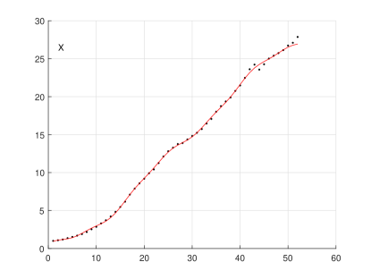
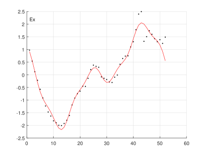
Figure 1: Modelling curves of gross outputs (left) and fluctuation of gross output (right) of all economy.

The graphics show points that give statistical information and the solid line is the trajectory. Comparison of the predicted values with the real data (the last two points, which correspond to years $2016$ and $2017$), testifies that the model has high accuracy predictive properties.

Analysis of modelling curves shows that they give a qualitative approximation of statistical data. Therefore, the proposed method can be used for effective forecasting in real macroeconomic systems. Investigating the economy of France, we have received the following modelling trajectory:

$$\begin{split}x(t)&=-7.10705+3.3429t+7.2722\cos(\omega_{1}t)-8.898\sin(\omega_{1}t)\\ &\quad+4.4042\cos(\omega_{2}t)-4.1148\sin(\omega_{2}t)-1.3436\cos(\omega_{3}t)\\ &\quad-0.1239\sin(\omega_{3}t)+0.2233\sin(\omega_{6}t)-0.0976\sin(\omega_{6}t)\;.\end{split}$$

Let us analyse the harmonics that are present in this modelling trajectory and, therefore, have an influence on the macroeconomic system of France. Figure 2 shows the graphics of the first, second, third, and sixth harmonics within the interval $t\in[35,80]$, that is, from years 2000 to 2045.

t]

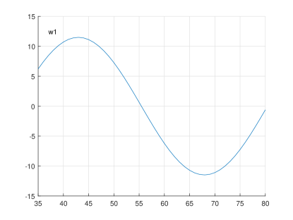
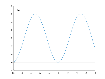
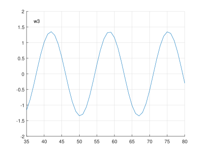
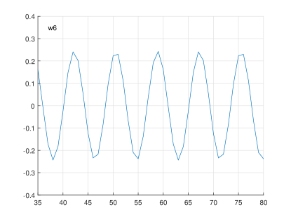
Figure 2: Modelling the harmonic waves for the economy of France.

The analysis shows that since $2000$, the first three harmonics are in the lifting phase. Since $2003$, it is supplemented by the $6$th harmonic lifting phase. So this period can be considered as the “golden era” of France. But in $2008$, the $1$st, $3$rd, and $4$th harmonics entered a phase of decline. As a result, at the end of $2008$, the economic crisis has begun. The cause of the crisis was the fact that all the basic harmonics entered into the phase of decline. It is supplemented by the $2$nd harmonic since $2012$. Further analysis shows the $6$th harmonic will enter the growth phase in $2020$. The $3$rd harmonic is in lifting phase now and until $2024$, when the wave starts to decline. The analysis of the $2$nd wave shows that it is now in a phase of decline. Changes are expected to begin in $2025$, when the $2$nd wave enters the growing phase until $2040$. However, significant changes should be expected starting with the year $2034$, when the Kondratieff wave will enter the phase of lifting. In $2034$, it will be supplemented with the $3$rd harmonic, in $2037$ with the $6$th harmonics. Therefore, after that time, we observe a gradual growth of the economic development of France.

5 Conclusions

The constructed mechanism, for simulation and forecasting dynamics of a macroeconomic system, allows to establish interconnections between individual economy sectors. The identification algorithm of the structural model of the inter-branch balance can be used for efficient allocation of resources in the formation of relationships between different branches. The resulting trajectories of issues and non-productive consumption have high imitation and forecast properties. The developed method can also be used for the analysis and forecasting development of real macroeconomic systems.

- (1) Leontief, W.: Input-Output Economics, Oxford University Press, New York, 1986.
- (2) Ramsay, J.O., Hooker, G., Campbell, D.: Parameter estimation for differential equations: A generalized smoothing approach, J. R. Stat. Soc. Ser. B Stat. Methodol. 69 (2007), no. 5, 741–796.
- (3) Nazarenko, O.M., Filchenko, D.V.: Parametric identification of state-space dynamic systems: A time-domain perspective, Int. J. of Innovating Computing, Information and Control. 4 (2008), no. 7, 1553–1566.
- (4) Kostylenko, O.O., Nazarenko, O.M: Modelling and identification of macroeconomic system dynamic interindustry balance, Mechanism of Economic Regulation 1(63) (2014), 76–86.
- (5) Kostylenko, O.O., Nazarenko, O.M: Identification of dynamic “input-output” model and forecasting of macroeconomic system, Novelties of Economic Cybernetics 3 (2013), 50–64.
- (6) Diebolt, C., Doliger, C.: Kondratieff Waves, Warfare and World Security. In: Economic Cycles Under Test: A Spectral Analysis, 39–47, IOS Press, Amsterdam, 2006.
- (7) Korotayev, A.V., Tsirel, S.V.: Spectral analysis of world GDP dynamics: Kondratieff waves, Kuznets swings, Juglar and Kitchin cycles in global economic development, and the 2008–2009 economic crisis, Structure and Dynamics 4 (2010), no. 1, 3–57.
- (8) Fied, B.C.: Environmental Economics: An Introduction, McGraw-Hill, New York, 1997.
- (9) Dobos, I., Floriska, A.: A dynamic Leontief model with non-renewable resources, Economics Systems Research 17 (2005), 319–328.
- (10) Nazarenko, O.M: Construction and identification of linear-quadratic models of weakly formalized dynamic systems (in Ukrainian), Math. Modelling Inform. Tech. Aut. Control Systems 10 (2008), no. 833, 185–192.
- (11) Greene, W.H.: Econometric Analysis, 5th ed., Pearson Educ. Int., N.Y., 2003.
- (12) INSEE, http://www.bdm.insee.fr/bdm2/index.action