Making Trotters Sprint: A Variational Imaginary Time Ansatz for Quantum Many-body Systems
Abstract
We introduce a variational wavefunction for many-body ground states that involves imaginary time evolution with two different Hamiltonians in an alternating fashion with variable time intervals. We successfully apply the ansatz on the one- and two-dimensional transverse-field Ising model and systematically study its scaling for the one-dimensional model at criticality. We find the total imaginary time required scales logarithmically with system size, in contrast to the linear scaling in conventional Quantum Monte Carlo. We suggest this is due to unique dynamics permitted by alternating imaginary time evolution, including exponential growth of bipartite entanglement. For generic models, the superior scaling of our ansatz potentially mitigates the negative sign problem at the expense of having to optimize variational parameters.
Introduction– Imaginary time plays a prominent role in multiple branches of physics, including cosmology, statistical mechanics and quantum field theory. The seemingly simple replacement of real time, , with its imaginary counterpart, , leads to fundamental connections between quantum theory and statistical mechanics Wick (1954). Such connections enable the efficient simulation of many quantum systems using quantum Monte Carlo techniques Handscomb (1962); Blankenbecler and Sugar (1983); Sandvik and Kurkijärvi (1991). However, for many physically interesting models, these methods suffer from the prohibitive ‘negative sign problem’ Loh et al. (1990); Troyer and Wiese (2005), which requires an exponential amount of computational resources to obtain reasonable accuracy for quantum many-body systems. Many outstanding problems in condensed matter, such as those involving high temperature superconductors or topologically ordered phases, require an understanding of complex interacting models which are unsolved with present techniques.
One class of Monte Carlo methods that can avoid the sign problem are so-called variational Monte Carlo (VMC) methods Gutzwiller (1963); *gutzwillerCorrelationElectronsNarrow1965; Ceperley et al. (1977); Otsuka (1992); Baeriswyl (1987); Becca and Sorella (2017). In VMC, one assumes a sufficiently general trial state that depends on adjustable parameters. These parameters are then chosen to minimize the energy with respect to the given Hamiltonian. Finding an effective trial state such as Jastrow Becca and Sorella (2017), matrix product states Verstraete et al. (2004); Sandvik and Vidal (2007); Vidal (2007), or neural network states Carleo and Troyer (2017); Freitas et al. (2018); Inack et al. (2018); Pilati et al. (2019), can result in efficient simulation of interacting quantum systems. The key to the success of these techniques is a well-chosen ansatz that reflects the properties of the target phase and the existence of a viable optimization scheme Umrigar et al. (1988); Sorella (1998); *sorellaGeneralizedLanczosAlgorithm2001; *sorellaWaveFunctionOptimization2005.
The recent advent of quantum computers and simulators has motivated the development of new variational approaches Jones et al. (2019). Such variational quantum algorithms involve applying a sequence of unitary operators, parameterized by several variables onto a easy-to-prepare initial state. The variables are chosen to optimize a given cost function involving the resulting wavefunction. For example, in the quantum approximate optimization algorithm (QAOA) Farhi et al. (2014); Zhou et al. (2018); Wang et al. (2018); Hadfield et al. (2019); Verdon et al. (2019) the cost function is a classical Hamiltonian encoding a combinatorial optimization problem, and the variational wavefunction is prepared by alternating between evolving with the Hamiltonian and a transverse field. The evolution times constitute variational parameters that are optimized to minimize the Hamiltonian cost function. This variational approach has been generalized for preparing both strongly correlated and highly-entangled states on near-term quantum devices Wecker et al. (2015); Ho and Hsieh (2019); Ho et al. (2019).
Motivated by the success of such variational approaches, in this Letter we propose a variational ansatz for ground states of quantum many-body systems which involves sequentially evolving with different Hamiltonians in imaginary time. In contrast to real time evolution with local Hamiltonians, which is limited by Lieb-Robinson bounds on the growth of correlation functions, imaginary time evolution does not have this constraint and can exhibit remarkable efficiency in traversing Hilbert space.
As proof of concept, we demonstrate the efficiency of our ansatz in representing the ground state of the transverse field Ising model at criticality. Whereas standard projector methods require imaginary time scaling with system size to reach the critical ground state, we show numerically that our ansatz requires time scaling logarithmically with . Furthermore, we analyze how entanglement grows after each imaginary time operation in our ansatz, and we find an exponential growth that is a unique feature of imaginary time dynamics. We conclude by demonstrating that the ansatz continues to perform well in the presence of integrability-breaking perturbations, and we mention generalizations of our ansatz to other models, including those with sign problems. We envision the main purpose of this ansatz to be an efficient trial wavefunction for quantum many-body physics on (classical) computers, however, it is possible that one can also implement such imaginary time evolution natively on a quantum computer McArdle et al. (2018); Motta et al. (2019).
Ansatz– Many Hamiltonians are naturally a linear combination of two components , where are individually tractable to analyze. Examples include transverse field Ising, Hubbard, and the – model. Motivated by the QAOA procedure, we consider the following variational imaginary time ansatz (VITA) for the ground state of :
| (1) |
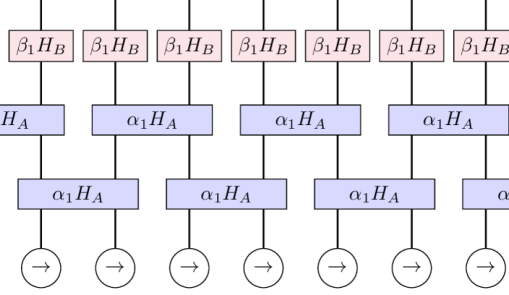
where is the number of pairs of variational parameters , is an initial state, and is a normalization factor. We further define the total imaginary time . A circuit representation is shown in Fig. 1. The bang-bang, or square-pulse, style of the ansatz is optimal for quantum control in real-time QAOA as per Pontryagin’s principle Yang et al. (2017).
While VITA is applicable to any Hamiltonian, in specific cases there is explicit physical motivation for considering such an ansatz. For example, for the fermionic Hubbard model, the ansatz reduces to Otsuka’s generalization of the Gutzwiller variational wavefunction Otsuka (1992); Gutzwiller (1963); *gutzwillerCorrelationElectronsNarrow1965; Baeriswyl (1987), which seeks to balance single occupancy per site with itinerancy. The case has been considered in Ref. Yanagisawa et al. (1998); *yanagisawaCrossoverWeaklyStrongly2016; *yanagisawaAntiferromagnetismSuperconductivityPhase2019 for the two-dimensional Hubbard model, but a systematic analysis of how its performance scales with system size and was not carried out. A related variational approach for the Hubbard model has also been considered in Ref. Vaezi and Vaezi (2018).
The standard projector method for attaining the ground state of involves evaluating for where is the many-body spectral gap. This can be decomposed via Trotterization into a sequence of the VITA form, with parameters for large . This guarantees that VITA can exactly represent the ground state in the limit. However, the projector method is especially expensive for critical systems where , and hence scales polynomially with . One can consider Eq. (1) as a non-uniform Trotterization with large (and variable) times steps. We will show that remarkably high fidelities can be attained even with that is exponentially smaller compared to the aforementioned estimate from the standard projector method.
We first present some general considerations of why such an ansatz may be efficient. It is useful to first compare with the real-time analogue, which are QAOA-type circuits involving alternating real-time evolution between two Hamiltonians. The Lieb-Robinson bound dictates that real-time evolution with local Hamiltonians can generate correlations only within a light cone, and thus there are lower bounds on the time it takes to prepare highly correlated states starting from unentangled product states. For example, in one dimension, the total time to prepare the GHZ (“cat”) state scales at least linearly with system size Bravyi et al. (2006); Ho and Hsieh (2019). In contrast, by evolving with the GHZ parent Hamiltonian in imaginary time ( is the Pauli- matrix), the GHZ state can be prepared with imaginary time scaling as 111See Supplemental Material.
Application– We test VITA on the transverse-field Ising model (TFIM)
| (2) |
with periodic boundary conditions on a system with spins. are the Pauli matrices, and is the transverse field strength. Our ansatz in this case starts from the paramagnetic ground state of , and alternates between and .
The Ising chain can be mapped to free fermions via the Jordan-Wigner transformation Lieb et al. (1961) which allows for the efficient evaluation of Eq. (1). We can thus optimize our ansatz for very large system sizes and several pulses. This allows us to properly characterize how efficient the VITA ansatz is without introducing sampling error. For a fixed , optimization involves finding the minima of the energy cost function .
We first focus on approximating the critical ground state of at . Figure 2a shows the relative error in energy where is the exact ground state energy at the critical point, for various . Evidently, increasing dramatically improves the accuracy in the energy, even for large system sizes. Optimized parameters for various are provided in supplementary material.
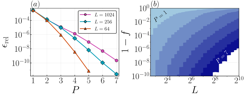
Since the exact ground state for the TFIM is known, we also compare the fidelity, , of the optimized trial state with the target state. The error in fidelity, , is shown in Fig. 2b for various . The efficiency is quite remarkable; for example, for , is already sufficient to approximate the critical state to within around in relative energy and in fidelity. Recall that the error in fidelity provides an upper-bound for the error in any observable 222See Supplemental Material.
Entanglement dynamics– While there is no Lieb-Robinson bound limiting the rate for generating long-range correlations in our ansatz, entanglement considerations provide lower bounds on the iterations required to prepare the critical state. Ignoring normalization, imaginary time evolution with a local Hamiltonian can be represented by a (non-unitary) quantum circuit; each iteration of our ansatz corresponds to three layers shown in Fig. 1. After pulses, the bipartite entanglement entropy between the left and right halves the system, hereafter abbreviated EE, can be attained by bisecting the circuit through bonds. Hence, EE after iterations is at most , where is the Schmidt rank (number of singular values) upon decomposing a single two-qubit imaginary time operator.
In order to generate the EE of the critical state, which scales as , we need the number of pulses scaling at least as . We observe that Fig. 2b is consistent with this scaling form. For example, for a target fidelity error of , each additional in the ansatz can represent a system approximately twice as large.
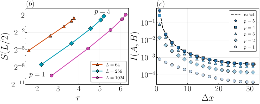
The entanglement dynamics in imaginary time evolution can be considerably different from its real time counterpart. For real time evolution, EE across a bipartition can increase only by acting with an operator supported on both sides of the partition. If the circuit in Fig. 1 were unitary, any increase in EE from one layer to the next would be bounded by a constant depending on the two-qubit unitary but not on the state being acted on (see the “small incremental entangling theorem” Mariën et al. (2014)). In contrast, even imaginary time operators acting on one side of the bipartition can generate entanglement across the cut. As a very simple example involving two spins, the action of on can increase EE as long as . This illustrates that the more entangled the initial state, the more imaginary time evolution can change the entanglement. The change is not simply bounded by a state-independent constant. This allows in principle an exponential growth of EE, as long as the total EE after steps lies below .
Our ansatz exhibits such dynamics. We take the ansatz and analyze the EE of the states at intermediate steps, , of our protocol using the technique of Peschel (2003); Vidal et al. (2003); *latorreGroundStateEntanglement2004. We find that the EE increases exponentially with imaginary time (Fig. 3a). Moreover, for every intermediate state, we plot the mutual information () between two spins as a function of their separation (Fig. 3b). The power law decay for every step is in stark contrast to any local real time evolution and illustrates the ability of imaginary time evolution to generate long-range correlations 333See Supplemental Material at [URL will be inserted by publisher] for considerations of a local quench in imaginary time in a conformal field theory . We find that under imaginary-time evolution, entanglement starts to grow immediately following a local quench, in contrast to real-time evolution Calabrese and Cardy (2005); *calabreseEntanglementCorrelationFunctions2007 where it takes a time proportional to before growing, being the distance between the location of the local quench and the entanglement cut.
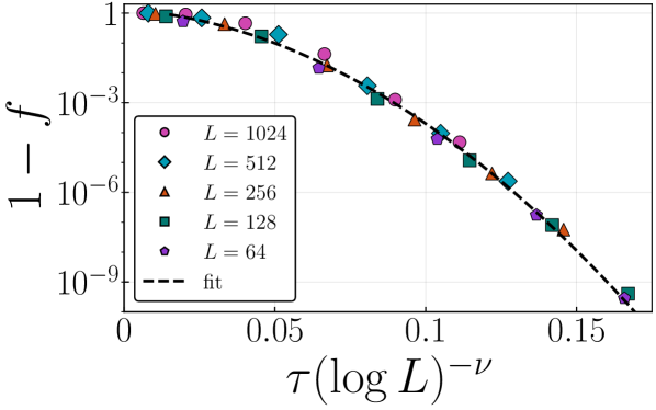
Scaling– To compare directly with the projector method, we also investigate the total imaginary time required to achieve a target fidelity. Motivated by the scaling for achieving a target fidelity, we propose a scaling form of for some exponent . We perform a scaling collapse for , and and find the optimal exponent . This logarithmic scaling is an exponential speedup compared to the linear scaling of the projector method, Liu et al. (2018).
Monte Carlo approach– While the TFIM model admits a dual representation as free fermions, for a general model sampling methods are crucial for estimating the energy cost function. As a proof of concept, we also use Monte Carlo sampling for stochastically optimizing VITA.
The quantum-classical correspondence maps quantum observables to dual classical observables of a classical anisotropic Ising model on an lattice. We denote the classical spin configurations by and the spatial and imaginary time by , respectively 444 This is a slight abuse of notation since in Eq. (1). However, this may be permitted since there are only unique time couplings due to the lattice symmetry..
The expectation value of a quantum observable is
| (3) |
where are dual classical observables, and is the Boltzmann weight corresponding to the Ising model with couplings between nearest neighbors in space and imaginary time, respectively. The couplings vary with imaginary time, , but are uniform in space. In this way, the energy of the trial wavefunction can be sampled efficiently with Monte Carlo.
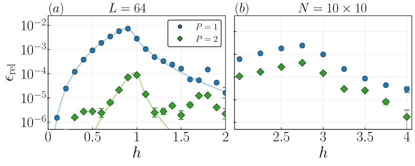
We use this scheme with to target the ground states for various values of the transverse field in both the (integrable) one-dimensional and the (non-integrable) two-dimensional TFIM. We use stochastic natural gradient descent (stochastic reconfiguration) to optimize the parameters Sorella (1998). We find rapid convergence for , while higher- becomes more difficult, especially for with a noisy objective function.
The relative error in energy achieved is shown in Fig. 5, with the free fermion results for comparison. For the VMC achieves the same accuracy as the free fermion method. However, for away from the critical point , the VMC performance is limited by sampling error 555 Of course the statistical error in Monte Carlo can be made arbitrarily small given long enough run-time since the sampling error goes as for Monte Carlo sweeps. This guarantees that VMC will converge to the free fermion solution in Fig. 5a if the globally optimal parameters can be found. The computational time of the MC sampling is where the autocorrelation time is a polynomial function of for spins and pulses of VITA. .
Discussion– We have introduced a variational technique that is motivated by both projector methods and recently developed quantum algorithms. It provides substantial shortcuts to the usual Trotterization of imaginary time evolution, at the expense of making the procedure variational. Using TFIM as a first testbed, we have demonstrated that this ansatz is viable for sampling methods and highly efficient. In particular, the number of variational parameters required to represent the TFIM critical state scales as , in contrast to other variational methods such as density matrix renormalization group (DMRG), which in this critical case requires bond dimension scaling with and thus number of parameters scaling with . One reason for this efficiency is the fact that imaginary time evolution is not subject to many bounds for real time evolution; despite being generated by local Hamiltonians, our ansatz exhibits an exponential growth of entanglement entropy and rapid generation of long-range correlations, features unique to imaginary time evolution.
Our variational approach is potentially useful in the many situations where imaginary time Trotterization involves a prohibitively large number of steps. For example, in models with a sign problem, the computational cost scales exponentially with space and imaginary time . Our ansatz provides a variational shortcut that significantly reduces (from to in the critical 1d TFIM) which could enable the study of larger systems even with a sign problem. For few variational parameters (), the optimization may be feasible, and we leave these investigations to future work.
Acknowledgements.
Acknowledgments– The authors would like to thank J. Carrasquilla, L. E. Hayward Sierens, E. Inack, B. Kulchytskyy, for many useful discussions. This research was supported by the Natural Sciences and Engineering Research Council of Canada (NSERC), the Canada Research Chair program, and the Perimeter Institute for Theoretical Physics. This work was made possible by the facilities of the Shared Hierarchical Academic Research Computing Network (SHARCNET) and Compute/Calcul Canada. Research at Perimeter Institute is supported by the Government of Canada through Industry Canada and by the Province of Ontario through the Ministry of Research & Innovation. TG is supported by the National Science Foundation under Grant No. DMR-1752417, and as an Alfred P. Sloan Research Fellow. This research was supported in part by the National Science Foundation under Grant No. NSF PHY-1748958.References
- Wick (1954) G. C. Wick, “Properties of Bethe-Salpeter Wave Functions,” Physical Review 96, 1124–1134 (1954).
- Handscomb (1962) D. C. Handscomb, “The Monte Carlo method in quantum statistical mechanics,” Mathematical Proceedings of the Cambridge Philosophical Society 58, 594–598 (1962).
- Blankenbecler and Sugar (1983) R. Blankenbecler and R. L. Sugar, “Projector Monte Carlo method,” Physical Review D 27, 1304–1311 (1983).
- Sandvik and Kurkijärvi (1991) Anders W. Sandvik and Juhani Kurkijärvi, “Quantum Monte Carlo simulation method for spin systems,” Physical Review B 43, 5950–5961 (1991).
- Loh et al. (1990) E. Y. Loh, J. E. Gubernatis, R. T. Scalettar, S. R. White, D. J. Scalapino, and R. L. Sugar, “Sign problem in the numerical simulation of many-electron systems,” Physical Review B 41, 9301–9307 (1990).
- Troyer and Wiese (2005) Matthias Troyer and Uwe-Jens Wiese, “Computational Complexity and Fundamental Limitations to Fermionic Quantum Monte Carlo Simulations,” Physical Review Letters 94, 170201 (2005).
- Gutzwiller (1963) Martin C. Gutzwiller, “Effect of Correlation on the Ferromagnetism of Transition Metals,” Physical Review Letters 10, 159–162 (1963).
- Gutzwiller (1965) Martin C. Gutzwiller, “Correlation of Electrons in a Narrow s Band,” Physical Review 137, A1726–A1735 (1965).
- Ceperley et al. (1977) D. Ceperley, G. V. Chester, and M. H. Kalos, “Monte Carlo simulation of a many-fermion study,” Physical Review B 16, 3081–3099 (1977).
- Otsuka (1992) Hiromi Otsuka, “Variational Monte Carlo Studies of the Hubbard Model in One- and Two-Dimensions –Off-Diagonal Intersite Correlation Effects–,” Journal of the Physical Society of Japan 61, 1645–1656 (1992).
- Baeriswyl (1987) D. Baeriswyl, “Variational Schemes for Many-Electron Systems,” in Nonlinearity in Condensed Matter, Springer Series in Solid-State Sciences, edited by Alan R. Bishop, David K. Campbell, Pradeep Kumar, and Steven E. Trullinger (Springer Berlin Heidelberg, 1987) pp. 183–193.
- Becca and Sorella (2017) Federico Becca and Sandro Sorella, Quantum Monte Carlo Approaches for Correlated Systems, 1st ed. (Cambridge University Press, Cambridge, United Kingdom ; New York, NY, 2017).
- Verstraete et al. (2004) F. Verstraete, D. Porras, and J. I. Cirac, “Density Matrix Renormalization Group and Periodic Boundary Conditions: A Quantum Information Perspective,” Physical Review Letters 93, 227205 (2004).
- Sandvik and Vidal (2007) A. W. Sandvik and G. Vidal, “Variational Quantum Monte Carlo Simulations with Tensor-Network States,” Physical Review Letters 99, 220602 (2007).
- Vidal (2007) G. Vidal, “Classical Simulation of Infinite-Size Quantum Lattice Systems in One Spatial Dimension,” Physical Review Letters 98, 070201 (2007).
- Carleo and Troyer (2017) Giuseppe Carleo and Matthias Troyer, “Solving the quantum many-body problem with artificial neural networks,” Science 355, 602 (2017).
- Freitas et al. (2018) Nahuel Freitas, Giovanna Morigi, and Vedran Dunjko, “Neural network operations and Susuki–Trotter evolution of neural network states,” International Journal of Quantum Information 16, 1840008 (2018).
- Inack et al. (2018) E. M. Inack, G. E. Santoro, L. Dell’Anna, and S. Pilati, “Projective quantum Monte Carlo simulations guided by unrestricted neural network states,” Physical Review B 98, 235145 (2018).
- Pilati et al. (2019) S. Pilati, E. M. Inack, and P. Pieri, “Self-learning projective quantum Monte Carlo simulations guided by restricted Boltzmann machines,” arXiv:1907.00907 [cond-mat] (2019).
- Umrigar et al. (1988) C. J. Umrigar, K. G. Wilson, and J. W. Wilkins, “Optimized trial wave functions for quantum Monte Carlo calculations,” Physical Review Letters 60, 1719–1722 (1988).
- Sorella (1998) S. Sorella, “Green Function Monte Carlo with Stochastic Reconfiguration,” Physical Review Letters 80, 4558–4561 (1998).
- Sorella (2001) S. Sorella, “Generalized Lanczos Algorithm for Variational Quantum Monte Carlo,” Physical Review B 64 (2001), 10/dz27zv.
- Sorella (2005) Sandro Sorella, “Wave function optimization in the variational Monte Carlo method,” Physical Review B 71, 241103 (2005).
- Jones et al. (2019) Tyson Jones, Suguru Endo, Sam McArdle, Xiao Yuan, and Simon C. Benjamin, “Variational quantum algorithms for discovering Hamiltonian spectra,” Physical Review A 99, 062304 (2019).
- Farhi et al. (2014) Edward Farhi, Jeffrey Goldstone, and Sam Gutmann, “A Quantum Approximate Optimization Algorithm,” arXiv:1411.4028 [quant-ph] (2014).
- Zhou et al. (2018) Leo Zhou, Sheng-Tao Wang, Soonwon Choi, Hannes Pichler, and Mikhail D. Lukin, “Quantum Approximate Optimization Algorithm: Performance, Mechanism, and Implementation on Near-Term Devices,” arXiv:1812.01041 [cond-mat, physics:quant-ph] (2018).
- Wang et al. (2018) Zhihui Wang, Stuart Hadfield, Zhang Jiang, and Eleanor G. Rieffel, “Quantum approximate optimization algorithm for MaxCut: A fermionic view,” Physical Review A 97, 022304 (2018).
- Hadfield et al. (2019) Stuart Hadfield, Zhihui Wang, Bryan O’Gorman, Eleanor G. Rieffel, Davide Venturelli, and Rupak Biswas, “From the Quantum Approximate Optimization Algorithm to a Quantum Alternating Operator Ansatz,” Algorithms 12, 34 (2019).
- Verdon et al. (2019) Guillaume Verdon, Juan Miguel Arrazola, Kamil Brádler, and Nathan Killoran, “A Quantum Approximate Optimization Algorithm for continuous problems,” arXiv:1902.00409 [quant-ph] (2019).
- Wecker et al. (2015) Dave Wecker, Matthew B. Hastings, and Matthias Troyer, “Progress towards practical quantum variational algorithms,” Physical Review A 92, 042303 (2015).
- Ho and Hsieh (2019) Wen Wei Ho and Timothy H. Hsieh, “Efficient variational simulation of non-trivial quantum states,” SciPost Physics 6, 029 (2019).
- Ho et al. (2019) Wen Wei Ho, Cheryne Jonay, and Timothy H. Hsieh, “Ultrafast variational simulation of nontrivial quantum states with long-range interactions,” Physical Review A 99, 052332 (2019).
- McArdle et al. (2018) Sam McArdle, Tyson Jones, Suguru Endo, Ying Li, Simon Benjamin, and Xiao Yuan, “Variational quantum simulation of imaginary time evolution,” arXiv:1804.03023 [quant-ph] (2018).
- Motta et al. (2019) Mario Motta, Chong Sun, Adrian Teck Keng Tan, Matthew J. O’ Rourke, Erika Ye, Austin J. Minnich, Fernando G. S. L. Brandao, and Garnet Kin-Lic Chan, “Quantum Imaginary Time Evolution, Quantum Lanczos, and Quantum Thermal Averaging,” arXiv:1901.07653 [quant-ph] (2019).
- Yang et al. (2017) Zhi-Cheng Yang, Armin Rahmani, Alireza Shabani, Hartmut Neven, and Claudio Chamon, “Optimizing Variational Quantum Algorithms Using Pontryagin’s Minimum Principle,” Physical Review X 7, 021027 (2017).
- Yanagisawa et al. (1998) Takashi Yanagisawa, Soh Koike, and Kunihiko Yamaji, “Off-Diagonal Wave Function Monte Carlo Studies of Hubbard Model I,” Journal of the Physical Society of Japan 67, 3867–3874 (1998).
- Yanagisawa (2016) Takashi Yanagisawa, “Crossover from Weakly to Strongly Correlated Regions in the Two-dimensional Hubbard Model — Off-diagonal Wave Function Monte Carlo Studies of Hubbard Model II —,” Journal of the Physical Society of Japan 85, 114707 (2016).
- Yanagisawa (2019) Takashi Yanagisawa, “Antiferromagnetism, Superconductivity and Phase Diagram in the Two-Dimensional Hubbard Model —Off-Diagonal Wave Function Monte Carlo Studies of Hubbard Model III—,” Journal of the Physical Society of Japan 88, 054702 (2019).
- Vaezi and Vaezi (2018) Mohammad-Sadegh Vaezi and Abolhassan Vaezi, “A unified theory of variational and quantum Monte Carlo methods and beyond,” arXiv:1810.00864 [cond-mat.str-el] (2018).
- Bravyi et al. (2006) S. Bravyi, M. B. Hastings, and F. Verstraete, “Lieb-Robinson Bounds and the Generation of Correlations and Topological Quantum Order,” Physical Review Letters 97, 050401 (2006).
- Note (1) See Supplemental Material.
- Lieb et al. (1961) Elliott Lieb, Theodore Schultz, and Daniel Mattis, “Two soluble models of an antiferromagnetic chain,” Annals of Physics 16, 407–466 (1961).
- Note (2) See Supplemental Material.
- Mariën et al. (2014) Michaël Mariën, Koenraad M. R. Audenaert, Karel Van Acoleyen, and Frank Verstraete, “Entanglement Rates and the Stability of the Area Law for the Entanglement Entropy,” arXiv:1411.0680 [math-ph] (2014).
- Peschel (2003) Ingo Peschel, “Calculation of reduced density matrices from correlation functions,” Journal of Physics A: Mathematical and General 36, L205–L208 (2003).
- Vidal et al. (2003) G. Vidal, J. I. Latorre, E. Rico, and A. Kitaev, “Entanglement in quantum critical phenomena,” Physical Review Letters 90 (2003), 10/chw37f.
- Latorre et al. (2004) J. I. Latorre, E. Rico, and G. Vidal, “Ground State Entanglement in Quantum Spin Chains,” Quantum Info. Comput. 4, 48–92 (2004).
- Note (3) See Supplemental Material at [URL will be inserted by publisher] for considerations of a local quench in imaginary time in a conformal field theory.
- Calabrese and Cardy (2005) Pasquale Calabrese and John Cardy, “Evolution of entanglement entropy in one-dimensional systems,” Journal of Statistical Mechanics: Theory and Experiment 2005, P04010 (2005).
- Calabrese and Cardy (2007) Pasquale Calabrese and John Cardy, “Entanglement and correlation functions following a local quench: A conformal field theory approach,” Journal of Statistical Mechanics: Theory and Experiment 2007, P10004–P10004 (2007).
- Liu et al. (2018) Lu Liu, Anders W. Sandvik, and Wenan Guo, “Typicality at quantum-critical points,” Chinese Physics B 27, 087501 (2018).
- Note (4) This is a slight abuse of notation since in Eq. (1). However, this may be permitted since there are only unique time couplings due to the lattice symmetry.
- Note (5) Of course the statistical error in Monte Carlo can be made arbitrarily small given long enough run-time since the sampling error goes as for Monte Carlo sweeps. This guarantees that VMC will converge to the free fermion solution in Fig. 5a if the globally optimal parameters can be found. The computational time of the MC sampling is where the autocorrelation time is a polynomial function of for spins and pulses of VITA.
- Sandvik (2005) Anders W. Sandvik, “Ground State Projection of Quantum Spin Systems in the Valence-Bond Basis,” Physical Review Letters 95, 207203 (2005).
- Sandvik (2003) Anders W. Sandvik, “Stochastic series expansion method for quantum Ising models with arbitrary interactions,” Physical Review E 68, 056701 (2003).