Fooling the Parallel Or Tester with Probability $8/27$

Abstract

It is well-known that the higher-order language PCF is not fully abstract: there is a program—the so-called parallel or tester, meant to test whether its input behaves as a parallel or—which never terminates on any input, operationally, but is denotationally non-trivial. We explore a probabilistic variant of PCF, and ask whether the parallel or tester exhibits a similar behavior there. The answer is no: operationally, one can feed the parallel or tester an input that will fool it into thinking it is a parallel or. We show that the largest probability of success of such would-be parallel ors is exactly $8/27$. The bound is reached by a very simple probabilistic program. The difficult part is to show that that bound cannot be exceeded.

1 Introduction

There is a recurring theme in security: to defeat a strong adversary, you need to rely on random choice. This paper will be a somewhat devious illustration of that principle, in the field of programming language semantics.

The higher-order, functional language PCF [Plo77] forms the core of actual programming languages such as Haskell [Bir98]. Plotkin [Plo77], and independently Sazonov [Saz76], had shown that PCF, while being adequate (i.e., its operational and denotational semantics match, in a precise sense), is not fully abstract: there are programs that are contextually equivalent (a notion arising from the operational semantics), but have different denotational semantics. (One should note that, conversely, two programs with the same denotational semantics are always contextually equivalent.)

The argument is as follows. In the denotational model, there is a function of type $\mathtt{int}\to\mathtt{int}\to\mathtt{int}$ called parallel or, which maps the pair $1,1$ to $1$, and both $0,N$ and $N,0$ to $0$, for whatever program $N$ (including non-terminating programs). One can show that parallel or is undefinable in PCF. More is true. One can define a PCF program, the parallel or tester, which takes an argument $f\colon\mathtt{int}\to\mathtt{int}\to\mathtt{int}$, and tests whether $f$ is a parallel or, by testing whether $f11=1$, $f0\Omega=0$, and $f\Omega 0=0$, where $\Omega$ is a canonical non-terminating program. The parallel or tester is contextually equivalent to the always non-terminating program $\lambda f.\Omega$, meaning that applying it to any PCF program (for $f$) will never terminate. However, the denotational semantics of the parallel or tester and of $\lambda f.\Omega$ differ: applied to any given parallel or map (which exists in the denotational model), one returns and the other one does not.

We introduce a probabilistic variant of PCF which we call PCF_P, and we define a suitable parallel or tester $\mathtt{portest}$. A PCF_P program $M$ fools the parallel or tester if $\mathtt{portest}$ applied to $M$ terminates. In PCF, there is no way of fooling the parallel or tester. Our purpose is to show that one can fool the parallel or tester of PCF_P with probability at most $8/27$, and that this bound is attained. The optimal fooler is easy to define. The hard part is to show that one cannot do better.

A final word before we start. Even though we started by motivating it from matters related to full abstraction, which involves both operational and denotational semantics, the question we are addressing is purely operational in nature: it is only concerned with the behavior of $\mathtt{portest}$ under its operational semantics, under arbitrary PCF_P contexts. Nonetheless, denotational semantics will be essential in our proof.

Outline. We define the syntax of $PCF_{\mathtt{P}}$ in Section 2, its operational semantics in Section 3, and—once we have stated the required basic facts we need from domain theory in Section 4—its denotational semantics in Section 5. We state the adequacy theorem at the end of the latter section. This says that the operational and denotational probabilities that a term $M$ of type $\mathtt{int}$ terminates on any given value $n\in\mathbb{Z}$ are the same. We define the parallel tester, and show that it can be fooled with probability $8/27$ at most, in Section 6. We conclude by citing some recent related work in Section 7.

2 The syntax of PCF_P

PCF_P is a typed language. The types are given by the grammar:

$$\sigma,\tau,\cdots ::=\mathtt{int}$$ basic types

$$\mid D\tau \tau$$ type of (subprobability) distributions on

$$\mid\sigma\to\tau \text{function types}.$$

Mathematically, $D\tau$ will be the type of subprobability valuations of elements of type $\tau$. Operationally, an element of type $D\tau$ is just a random value of type $\tau$. There is only one basic type, $\mathtt{int}$, but one could envision a more expressive algebra of datatypes.

A computation type is a type of the form $D\tau$ or $\sigma\to\tau$ where $\tau$ is a computation type. The computation types are the types where one can do computation, in particular whose objets can be defined by recursion.

Our language will have functions, and a function mapping inputs of type $\sigma$ to outputs of type $\tau$ will have type $\sigma\to\tau$. We write $\sigma_{1}\to\sigma_{2}\to\cdots\to\sigma_{n}\to\tau$ for $\sigma_{1}\to(\sigma_{2}\to(\cdots\to(\sigma_{n}\to\tau)\cdots))$, and this is a type of functions taking $n$ inputs, of respective types $\sigma_{1}$, $\sigma_{2}$, …, $\sigma_{n}$ and returning outputs of type $\tau$.

We fix a countably infinite set of variables $x_{\tau}$, $y_{\tau}$, $z_{\tau}$, …, for each type $\tau$. Each variable has a unique type, which we read off from its subscript. We will occasionally omit the type subscript when it is clear from context, or irrelevant.

$$\begin{array}[]{c@{\qquad}c}{tensy\vbox{\hbox spread0.0pt{\hskip 0.0pt plus 0.0001fil\hbox{\kern 9.04518pt\hbox{$\displaystyle\penalty 1$}}\hskip 0.0pt plus 0.0001fil}\hbox{\hbox{\kern 0.0pt\vrule height=0.25002pt,depth=0.25002pt,width=18.09036pt\hbox{}}}\hbox{\kern 0.0pt\hbox{$\displaystyle x_{\tau}\colon\tau$}}}}\qquad{tensy\vbox{\hbox spread0.0pt{\hskip 0.0pt plus 0.0001fil\hbox{\kern 11.75116pt\hbox{$\displaystyle\penalty 1$}}\hskip 0.0pt plus 0.0001fil}\hbox{\hbox{\kern 0.0pt\vrule height=0.25002pt,depth=0.25002pt,width=23.50232pt\hbox{\kern 3.00003pt$(n\in\mathbb{Z})$}}}\hbox{\kern 0.0pt\hbox{$\displaystyle n\colon\mathtt{int}$}}}}&{tensy\vbox{\hbox spread0.0pt{\hskip 0.0pt plus 0.0001fil\hbox{\kern 1.97221pt\hbox{$\displaystyle\penalty 1M\colon\mathtt{int}$}}\hskip 0.0pt plus 0.0001fil}\hbox{\hbox{\kern 0.0pt\vrule height=0.25002pt,depth=0.25002pt,width=32.23605pt\hbox{}}}\hbox{\kern 0.0pt\hbox{$\displaystyle{\mathtt{s}}M\colon\mathtt{int}$}}}}\qquad{tensy\vbox{\hbox spread0.0pt{\hskip 0.0pt plus 0.0001fil\hbox{\kern 2.77779pt\hbox{$\displaystyle\penalty 1M\colon\mathtt{int}$}}\hskip 0.0pt plus 0.0001fil}\hbox{\hbox{\kern 0.0pt\vrule height=0.25002pt,depth=0.25002pt,width=33.8472pt\hbox{}}}\hbox{\kern 0.0pt\hbox{$\displaystyle{\mathtt{p}}M\colon\mathtt{int}$}}}}\\ \\ {tensy\vbox{\hbox spread0.0pt{\hskip 0.0pt plus 0.0001fil\hbox{\kern 5.89758pt\hbox{$\displaystyle\penalty 1M\colon\mathtt{int}\quad N\colon\tau\quad P\colon\tau$}}\hskip 0.0pt plus 0.0001fil}\hbox{\hbox{\kern 0.0pt\vrule height=0.25002pt,depth=0.25002pt,width=102.43031pt\hbox{}}}\hbox{\kern 0.0pt\hbox{$\displaystyle\mathop{\mathtt{if}}\nolimits{M}=0\;\mathtt{then}\;{N}\;\mathbin{\mathtt{else}}{P}\colon\tau$}}}}&{tensy\vbox{\hbox spread0.0pt{\hskip 0.0pt plus 0.0001fil\hbox{$\displaystyle\penalty 1M\colon\tau\to\tau$}\hskip 0.0pt plus 0.0001fil}\hbox{\hbox{\kern 0.0pt\vrule height=0.25002pt,depth=0.25002pt,width=38.42337pt\hbox{\kern 3.00003pt$(\tau\text{ computation type})$}}}\hbox{\kern 6.18906pt\hbox{$\displaystyle\mathop{\mathtt{rec}}\nolimits_{\tau}M$}}}}\\ \\ {tensy\vbox{\hbox spread0.0pt{\hskip 0.0pt plus 0.0001fil\hbox{$\displaystyle\penalty 1M\colon\sigma\to\tau\quad N\colon\sigma$}\hskip 0.0pt plus 0.0001fil}\hbox{\hbox{\kern 0.0pt\vrule height=0.25002pt,depth=0.25002pt,width=72.93828pt\hbox{}}}\hbox{\kern 20.15845pt\hbox{$\displaystyle MN\colon\tau$}}}}&{tensy\vbox{\hbox spread0.0pt{\hskip 0.0pt plus 0.0001fil\hbox{\kern 17.73126pt\hbox{$\displaystyle\penalty 1M\colon\tau$}}\hskip 0.0pt plus 0.0001fil}\hbox{\hbox{\kern 0.0pt\vrule height=0.25002pt,depth=0.25002pt,width=58.95892pt\hbox{}}}\hbox{\kern 0.0pt\hbox{$\displaystyle\lambda x_{\sigma}.M\colon\sigma\to\tau$}}}}\\ \\ {tensy\vbox{\hbox spread0.0pt{\hskip 0.0pt plus 0.0001fil\hbox{$\displaystyle\penalty 1M\colon D\tau\quad N\colon D\tau$}\hskip 0.0pt plus 0.0001fil}\hbox{\hbox{\kern 0.0pt\vrule height=0.25002pt,depth=0.25002pt,width=72.44002pt\hbox{}}}\hbox{\kern 9.51978pt\hbox{$\displaystyle M\oplus N\colon D\tau$}}}}\qquad{tensy\vbox{\hbox spread0.0pt{\hskip 0.0pt plus 0.0001fil\hbox{\kern 12.00343pt\hbox{$\displaystyle\penalty 1M\colon\sigma$}}\hskip 0.0pt plus 0.0001fil}\hbox{\hbox{\kern 0.0pt\vrule height=0.25002pt,depth=0.25002pt,width=48.84586pt\hbox{}}}\hbox{\kern 0.0pt\hbox{$\displaystyle\mathop{\mathtt{ret}}\nolimits_{\sigma}M\colon D\sigma$}}}}&{tensy\vbox{\hbox spread0.0pt{\hskip 0.0pt plus 0.0001fil\hbox{$\displaystyle\penalty 1M\colon D\sigma\quad N\colon\sigma\to D\tau$}\hskip 0.0pt plus 0.0001fil}\hbox{\hbox{\kern 0.0pt\vrule height=0.25002pt,depth=0.25002pt,width=90.05217pt\hbox{}}}\hbox{\kern 11.26846pt\hbox{$\displaystyle\mathop{\mathtt{bind}}\nolimits_{\sigma,\tau}MN\colon D\tau$}}}}\end{array}$$

Figure 1: The syntax of PCF_P

The terms $M$, $N$, …, of our language are defined inductively, together with their types, in Figure 1. We agree to write $M\colon\tau$ to mean “$M$ is a term, of type $\tau$”. We shall write $MN_{1}N_{2}\cdots N_{n}$ for $(\cdots((MN_{1})N_{2})\cdots)N_{n}$, and $\lambda x_{1},\cdots,x_{n}.M$ for $\lambda x_{1}.\lambda x_{2}.\cdots.\lambda x_{n}.M$. We shall also use the abbreviations $\mathtt{let}\;{x_{\sigma}=M}\;\mathtt{in}\;{N}$ for $(\lambda x_{\sigma}.N)M$ and $\mathtt{letrec}\;{f_{\tau}=M}\;\mathtt{in}\;{N}$, where $M\colon\tau$, for $\mathtt{let}\;{f_{\tau}=\mathop{\mathtt{rec}}\nolimits\;{(}\lambda f_{\tau}.M)}\;\mathtt{in}\;{N}$. Finally, we shall write $\mathop{\mathtt{do}}{x_{\sigma}\leftarrow M};N$ for $\mathop{\mathtt{bind}}\nolimits_{\sigma,\tau}M(\lambda x_{\sigma}.N)$, of type $D\tau$ (draw $x_{\sigma}$ at random along distribution $M$, then run $N$). $M\oplus N$ is meant to execute either $M$ or $N$ with probability $1/2$.

The free variables and the bound variables of a term $M$ are defined as usual. A term with no free variable is ground. For a substitution $\theta\mathrel{\buildrel\text{def}\over{=}}[x_{1}:=N_{1},\cdots,x_{k}:=N_{k}]$ (where each $N_{i}$ has the same type as $x_{i}$, and the variables $x_{i}$ are pairwise distinct), we write $M\theta$ for the parallel substitution of each $N_{i}$ for each $x_{i}$, and $\mathop{\mathrm{dom}}\theta$ for $\{x_{1},\cdots,x_{k}\}$. We say that $\theta$ is ground if $N_{1}$, …, $N_{k}$ are all ground.

Example 2.1

The term $\mathtt{rand\_int}\mathrel{\buildrel\text{def}\over{=}}\mathop{\mathtt{rec}}\nolimits_{\mathtt{int}\to D\mathtt{int}}(\lambda r.\lambda m_{\mathtt{int}}.r({\mathtt{s}}m)\oplus\allowbreak\mathop{\mathtt{ret}}\nolimits_{\mathtt{int}}m)0$ is of type $D\mathtt{int}$. As we will see, this draws a natural number $n$ at random, with probability $1/2^{n+1}$.

Example 2.2

Rejection sampling is a process by which one draws an element of a subset $A$ of a space $X$, as follows: we draw an element of $X$ at random, and we return it if it lies in $A$, otherwise we start all over again. Here is a simple example of rejection sampling, meant to draw a number uniformly among $\{0,1,2\}$. The idea is to draw two independent bits at random, representing a number in $X\mathrel{\buildrel\text{def}\over{=}}\{0,1,2,3\}$, and to use rejection sampling on $A\mathrel{\buildrel\text{def}\over{=}}\{0,1,2\}$. Formally, we define the PCF_P term $\mathtt{rand3}\mathrel{\buildrel\text{def}\over{=}}\mathop{\mathtt{rec}}\nolimits_{D\mathtt{int}}(\lambda p_{D\mathtt{int}}.((\mathop{\mathtt{ret}}\nolimits_{\mathtt{int}}0\oplus\mathop{\mathtt{ret}}\nolimits_{\mathtt{int}}1)\oplus(\mathop{\mathtt{ret}}\nolimits_{\mathtt{int}}2\oplus p_{D\mathtt{int}})))$. Note that this uses recursion to define a distribution, not a function.

3 Operational semantics

The elementary contexts $E$, with their types $\sigma\vdash\tau$, are defined as:

• $[\_N]$ of type $(\sigma\to\tau)\vdash\tau$, for every $N\colon\sigma$, and for every type $\tau$;

• $[{\mathtt{s}}\_]$ and $[{\mathtt{p}}\_]$, of type $\mathtt{int}\vdash\mathtt{int}$;

• $[\mathop{\mathtt{if}}\nolimits{\_}=0\;\mathtt{then}\;{N}\;\mathbin{\mathtt{else}}{P}]$, of type $\mathtt{int}\vdash\tau$, for all $N,P\colon\tau$;

• $[\mathop{\mathtt{bind}}\nolimits_{\sigma,\tau}\_N]$, of type $D\sigma\vdash D\tau$, for every $N\colon\sigma\to D\tau$.

The initial contexts are $[\_]$ (of type $\sigma\vdash\sigma$ for any $\sigma$) and $[\mathop{\mathtt{ret}}\nolimits_{\mathtt{int}}\_]$ (of type $\mathtt{int}\vdash D\mathtt{int}$). The (evaluation) contexts $C$ are the finite sequences $E_{0}E_{1}\cdots E_{n}$, $n\in\mathbb{N}$, where $E_{0}$ is an initial context of type $\sigma_{1}\vdash\sigma_{0}$, each $E_{i}$ ($1\leq i\leq n$) is an elementary context of type $\sigma_{i+1}\vdash\sigma_{i}$. Then we say that $C$ has type $\sigma_{n+1}\vdash\sigma_{0}$.

The notation $C[M]$ makes sense for every context $C\mathrel{\buildrel\text{def}\over{=}}E_{0}E_{1}\cdots E_{n}$ of type $\sigma\vdash\tau$ and every $M\colon\sigma$, and is defined as $E_{0}[E_{1}[\cdots[E_{n}[M]]]]$, where $E[M]$ is defined by removing the square brackets in $E$ and replacing the hole $\_$ by $M$. E.g., if $C=[\mathop{\mathtt{ret}}\nolimits_{\mathtt{int}}\_][{\mathtt{p}}\_]$, then $C[M]=\mathop{\mathtt{ret}}\nolimits_{\mathtt{int}}({\mathtt{p}}M)$.

$$\begin{array}[]{cc}\hline\cr\lx@intercol\hfil\text{Exploration rules}\hfil\lx@intercol\\ \hline\cr C\cdot E[M]\mathrel{\buildrel 1\over{\to}}CE\cdot M\quad\text{($E$ elem.\ context)}&[\_]\cdot\mathop{\mathtt{ret}}\nolimits_{\mathtt{int}}M\mathrel{\buildrel 1\over{\to}}[\mathop{\mathtt{ret}}\nolimits_{\mathtt{int}}\_]\cdot M\\ \hline\cr\hline\cr\lx@intercol\hfil\text{Computation rules}\hfil\lx@intercol\\ \hline\cr C[\_N]\cdot\lambda x_{\sigma}.M\mathrel{\buildrel 1\over{\to}}C\cdot M[x_{\sigma}:=N]&C\cdot\mathop{\mathtt{rec}}\nolimits_{\tau}M\mathrel{\buildrel 1\over{\to}}C\cdot M(\mathop{\mathtt{rec}}\nolimits_{\tau}M)\\ C\cdot M\oplus N\mathrel{\buildrel 1/2\over{\to}}C\cdot M&C\cdot M\oplus N\mathrel{\buildrel 1/2\over{\to}}C\cdot N\\ C[\mathop{\mathtt{bind}}\nolimits_{\sigma,\tau}\_N]\cdot\mathop{\mathtt{ret}}\nolimits_{\sigma}M\mathrel{\buildrel 1\over{\to}}C\cdot NM&C[{\mathtt{p}}\_]\cdot n\mathrel{\buildrel 1\over{\to}}C\cdot n-1\quad C[{\mathtt{s}}\_]\cdot n\mathrel{\buildrel 1\over{\to}}C\cdot n+1\\ C[\mathop{\mathtt{if}}\nolimits{\_}=0\;\mathtt{then}\;{N}\;\mathbin{\mathtt{else}}{P}]\cdot 0\mathrel{\buildrel 1\over{\to}}C\cdot N&C[\mathop{\mathtt{if}}\nolimits{\_}=0\;\mathtt{then}\;{N}\;\mathbin{\mathtt{else}}{P}]\cdot n\mathrel{\buildrel 1\over{\to}}C\cdot P\quad(n\neq 0)\\ \hline\cr\end{array}$$

Figure 2: Operational semantics

A configuration (of type $\tau$) is a pair $C\cdot M$, where $C$ is a context of type $\sigma\vdash\tau$ and $M\colon\sigma$.

The operational semantics of PCF_P—an abstract interpreter that runs PCF_P programs—is a probabilistic transition system on configurations, defined by the rules of Figure 2. We write $s\mathrel{\buildrel\alpha\over{\to}}s^{\prime}$ to say that one can go from configuration $s$ to configuration $s^{\prime}$ in one step, with probability $\alpha$.

A trace is a sequence $s_{0}\mathrel{\buildrel\alpha_{1}\over{\to}}s_{1}\mathrel{\buildrel\alpha_{2}\over{\to}}\cdots\mathrel{\buildrel\alpha_{m}\over{\to}}s_{m}$, where $m\in\mathbb{N}$, and where each $s_{i-1}\mathrel{\buildrel\alpha_{i}\over{\to}}s_{i}$ is an instance of a rule of Figure 2. The trace starts at $s_{0}$, ends at $s_{m}$, its length is $m$ and its weight is the product $\alpha\mathrel{\buildrel\text{def}\over{=}}\alpha_{1}\cdots\alpha_{2}\cdots\alpha_{m}$. In that case, we also write $s_{0}\mathrel{\buildrel\alpha\over{\to}{}^{*}}s_{m}$.

The run starting at $s_{0}$ is the tree of all traces starting at $s_{0}$. Its root is $s_{0}$ itself, and for each vertex $s$ in the tree, for each instance of a rule of the form $s\mathrel{\buildrel\alpha\over{\to}}t$, $t$ is a successor of $s$, and the edge from $s$ to $t$ is labeled $\alpha$.

Figure 3: An example run in PCF_P

For every configuration $s$ of type $D\mathtt{int}$, and every $n\in\mathbb{Z}$, we define $\mathop{\text{Pr}}[s\mathbin{\downarrow}n]$ as the sum of the weights of all traces that start at $s$ and end at $[\mathop{\mathtt{ret}}\nolimits_{\mathtt{int}}\_]\cdot n$. This is the subprobability that $s$ eventually computes $n$. We also write $\mathop{\text{Pr}}[M\mathbin{\downarrow}n]$ for $\mathop{\text{Pr}}[[\_]\cdot M\mathbin{\downarrow}n]$, where $M\colon D\mathtt{int}$.

Example 3.1

The run starting at $\mathtt{rand\_int}$ (see Example 2.1) is shown in Figure 3. We have abbreviated some sequences of $\mathrel{\buildrel 1\over{\to}}$ steps as $\mathrel{\buildrel 1\over{\to}{}^{*}}$. One sees that $\mathop{\text{Pr}}[\mathtt{rand\_int}\mathbin{\downarrow}n]=1/2^{n+1}$ for every $n\in\mathbb{N}$, and is zero for every $n<0$. Notice the infinite branch on the left, whose weight is $0$.

Example 3.2

We let the reader draw the run starting at $\mathtt{rand3}$ (see Example 2.2), and check that $\mathop{\text{Pr}}[\mathtt{rand3}\mathbin{\downarrow}n]$ is equal to $1/3$ if $n\in\{0,1,2\}$, $0$ otherwise. Explicitly, if $n\in\{0,1,2\}$, show that the traces that start at $\mathtt{rand3}$ and end at $[\mathop{\mathtt{ret}}\nolimits_{\mathtt{int}}\_]\cdot n$ have respective weights $1/4$, $1/4\cdot 1/4$, …, $(1/4)^{n}\cdot 1/4$, …, and that the sum of those weights is $1/3$.

The following is immediate.

Lemma 3.3

The following hold:

1. For every rule $s\mathrel{\buildrel\alpha\over{\to}}t$, $t$ and $s$ have the same type.

2. For every rule of the form $s\mathrel{\buildrel 1\over{\to}}t$ of type $D\mathtt{int}$, for every $n\in\mathbb{Z}$, $\mathop{\text{Pr}}[t\mathbin{\downarrow}n]=\mathop{\text{Pr}}[s\mathbin{\downarrow}n]$.

3. $\mathop{\text{Pr}}[C\cdot M\oplus N\mathbin{\downarrow}n]=\frac{1}{2}\mathop{\text{Pr}}[C\cdot M\mathbin{\downarrow}n]+\frac{1}{2}\mathop{\text{Pr}}[C\cdot N\mathbin{\downarrow}n]$. $\Box$

4 A refresher on domain theory

We will require some elementary domain theory, for which we refer the reader to [GHK⁺03, AJ94, Gou13]. A poset $X$ is a set with a partial ordering, which we will always write as $\leq$. A directed family $D\subseteq X$ is a non-empty family such that every pair of points of $D$ has an upper bound in $D$. A dcpo is a poset in which every directed family $D$ has a supremum $\sideset{}{{}^{\,\makebox[0.0pt]{$\scriptstyle\uparrow$}\!}}{\sup}D$. If $D={(x_{i})}_{i\in I}$, we also write $\sideset{}{{}^{\,\makebox[0.0pt]{$\scriptstyle\uparrow$}\!}}{\sup}_{i\in I}x_{i}$ for $\sideset{}{{}^{\,\makebox[0.0pt]{$\scriptstyle\uparrow$}\!}}{\sup}D$.

The product $X\times Y$ of two dcpos is the set of pairs $(x,y)$, $x\in X$, $y\in Y$, ordered by $(x,y)\leq(x^{\prime},y^{\prime})$ if and only if $x\leq x^{\prime}$ and $y\leq y^{\prime}$.

For any two dcpos $X$ and $Y$, a map $f\colon X\to Y$ is Scott-continuous if and only if it is monotonic ($x\leq x^{\prime}$ implies $f(x)\leq f(x^{\prime})$) and preserves directed suprema (for every directed family ${(x_{i})}_{i\in I}$ in $X$, $\sideset{}{{}^{\,\makebox[0.0pt]{$\scriptstyle\uparrow$}\!}}{\sup}_{i\in I}f(x_{i})=f(\sideset{}{{}^{\,\makebox[0.0pt]{$\scriptstyle\uparrow$}\!}}{\sup}_{i\in I}x_{i})$). There is a category $\mathbf{Dcpo}$ of dcpos and Scott-continuous maps.

We order maps from $X$ to $Y$ by $f\leq g$ if and only if $f(x)\leq g(x)$ for every $x\in X$. The poset $[X\to Y]$ of all Scott-continuous maps from $X$ to $Y$ is then again a dcpo, and directed suprema are computed pointwise: $(\sideset{}{{}^{\,\makebox[0.0pt]{$\scriptstyle\uparrow$}\!}}{\sup}_{i\in I}f_{i})(x)=\sideset{}{{}^{\,\makebox[0.0pt]{$\scriptstyle\uparrow$}\!}}{\sup}_{i\in I}(f_{i}(x))$. $\mathbf{Dcpo}$ is a Cartesian-closed category—a model of simply-typed $\lambda$-calculus—and that can be said more concretely as follows:

• for all dcpos $X$, $Y$, there is a Scott-continuous map $\text{{App}}\colon[X\to Y]\times X\to Y$ defined by $\text{{App}}(f,x)\mathrel{\buildrel\text{def}\over{=}}f(x)$;

• for all dcpos $X$, $Y$, $Z$, for every Scott-continuous map $f\colon Z\times X\to Y$, the map $\Lambda_{X}(f)\colon Z\to[X\to Y]$ defined by $\Lambda_{X}(f)(z)(x)\mathrel{\buildrel\text{def}\over{=}}f(z,x)$ is Scott-continuous;

• those satisfy certain equations which we will not require.

If the dcpo $X$ is pointed, namely if it has a least element $\bot$, then every Scott-continuous map $f\colon X\to X$ has a least fixed point $\mathop{\mathrm{lfp}}\nolimits_{X}(f)\mathrel{\buildrel\text{def}\over{=}}\sideset{}{{}^{\,\makebox[0.0pt]{$\scriptstyle\uparrow$}\!}}{\sup}_{n\in\mathbb{N}}f^{n}(\bot)$. This is used to interpret recursion. Additionally, the map $\mathop{\mathrm{lfp}}\nolimits_{X}\colon[X\to X]\to X$ is itself Scott-continuous.

The set $\overline{\mathbb{R}}_{+}\mathrel{\buildrel\text{def}\over{=}}\mathbb{R}_{+}\cup\{\infty\}$ of extended non-negative real numbers is a dcpo under the usual ordering. We write ${\mathcal{L}}X$ for $[X\to\overline{\mathbb{R}}_{+}]$. Its elements are called the lower semicontinuous functions in analysis.

A Scott-open subset $U$ of a dcpo $X$ is an upwards-closed subset ($x\in U$ and $x\leq y$ imply $y\in U$) that is inaccessible from below (every directed family $D$ such that $\sideset{}{{}^{\,\makebox[0.0pt]{$\scriptstyle\uparrow$}\!}}{\sup}D\in U$ intersects $U$). The lattice of Scott-open subsets is written $\mathcal{O}X$, and forms a topology, the Scott topology on $X$. Note that $\mathcal{O}X$ is itself a dcpo under inclusion, and directed suprema are computed as unions.

The Scott-closed sets are the complements of Scott-open sets, i.e., the downwards-closed subsets $C$ such that for every directed family $D\subseteq C$, $\sideset{}{{}^{\,\makebox[0.0pt]{$\scriptstyle\uparrow$}\!}}{\sup}D\in C$.

In order to give a denotational semantics to probabilistic choice, we will follow Jones [JP89, Jon90]. A continuous valuation on $X$ is a map $\nu\colon\mathcal{O}X\to\overline{\mathbb{R}}_{+}$ that is strict ($\nu(\emptyset)=0$), monotone ($U\subseteq V$ implies $\nu(U)\leq\nu(V)$), modular ($\nu(U)+\nu(V)=\nu(U\cup V)+\nu(U\cap V)$), and Scott-continuous ($\nu(\sideset{}{{}^{\,\makebox[0.0pt]{$\scriptstyle\uparrow$}\!}}{\bigcup}_{i\in I}U_{i})=\sideset{}{{}^{\,\makebox[0.0pt]{$\scriptstyle\uparrow$}\!}}{\sup}_{i\in I}\nu(U_{i})$). A subprobability valuation additionally satisfies $\nu(X)\leq 1$. Continuous valuations and measures are very close concepts: see [KL05] for details.

Among subprobability valuations, one finds the Dirac valuation $\delta_{x}$, for each $x\in X$, defined by $\delta_{x}(U)\mathrel{\buildrel\text{def}\over{=}}1$ if $x\in U$, $0$ otherwise. One can integrate any Scott-continuous map $f\colon X\to\overline{\mathbb{R}}_{+}$, and the integral $\int_{x\in X}f(x)d\nu$ is Scott-continuous and linear (i.e., commutes with sums and scalar products by elements of $\mathbb{R}_{+}$) both in $f$ and in $\nu$.

We write $\mathbf{V}_{\leq 1}X$ for the poset of subprobability valuations on $X$. This is a dcpo under the pointwise ordering ($\mu\leq\nu$ if and only if $\mu(U)\leq\nu(U)$ for every $U\in\mathcal{O}X$), and directed suprema are computed pointwise ($(\sideset{}{{}^{\,\makebox[0.0pt]{$\scriptstyle\uparrow$}\!}}{\sup}_{i\in I}\nu_{i})(U)=\sideset{}{{}^{\,\makebox[0.0pt]{$\scriptstyle\uparrow$}\!}}{\sup}_{i\in I}(\nu_{i}(U))$). Additionally, $\mathbf{V}_{\leq 1}$ defines a monad on $\mathbf{Dcpo}$. Concretely:

• there is a unit $\eta\colon X\to\mathbf{V}_{\leq 1}X$, which is the continuous map $x\mapsto\delta_{x}$;

• every Scott-continuous map $f\colon X\to\mathbf{V}_{\leq 1}Y$ has an extension $f^{\dagger}\colon\mathbf{V}_{\leq 1}X\to\mathbf{V}_{\leq 1}Y$, defined by $f^{\dagger}(\nu)(V)\mathrel{\buildrel\text{def}\over{=}}\int_{x\in X}f(x)(V)d\nu$;

• those satisfy a certain number of equations, of which we will need the following:

  $$f^{\dagger}(\eta(x)) =f(x)$$ (1)

  $$\int_{y\in Y}h(y)df^{\dagger}(\nu) =\int_{x\in X}\left(\int_{y\in Y}h(y)df(x)\right)d\nu,$$ (2)

  for all Scott-continuous maps $f\colon X\to Y$, $h\colon Y\to\overline{\mathbb{R}}_{+}$, and every $\nu\in\mathbf{V}_{\leq 1}X$.

Note that the map $f\mapsto f^{\dagger}$ is itself Scott-continuous.

5 Denotational semantics

The types $\tau$ are interpreted as dcpos $\left\llbracket{\tau}\right\rrbracket$, as follows: $\left\llbracket{\mathtt{int}}\right\rrbracket\mathrel{\buildrel\text{def}\over{=}}\mathbb{Z}$, with equality as ordering; $\left\llbracket{D\tau}\right\rrbracket\mathrel{\buildrel\text{def}\over{=}}\mathbf{V}_{\leq 1}\left\llbracket{\tau}\right\rrbracket$; and $\left\llbracket{\sigma\to\tau}\right\rrbracket\mathrel{\buildrel\text{def}\over{=}}[\left\llbracket{\sigma}\right\rrbracket\to\left\llbracket{\tau}\right\rrbracket]$. Note that $\left\llbracket{\tau}\right\rrbracket$ is pointed for every computation type $\tau$, so $\mathop{\mathrm{lfp}}\nolimits_{\left\llbracket{\tau}\right\rrbracket}$ makes sense in those cases.

An environment is a map $\rho$ sending each variable $x_{\tau}$ to an element $\rho(x_{\tau})$ of $\left\llbracket{\tau}\right\rrbracket$. The dcpo $Env$ of environments is the product $\prod_{x_{\tau}\text{ variable}}\left\llbracket{\tau}\right\rrbracket$, with the usual componentwise ordering. When $V\in\left\llbracket{\sigma}\right\rrbracket$, we write $\rho[x_{\sigma}:=V]$ for the environment that maps $x_{\sigma}$ to $V$, and all other variables $y$ to $\rho(y)$.

$$\begin{array}[]{c@{\quad}c}\left\llbracket{x_{\tau}}\right\rrbracket\rho\mathrel{\buildrel\text{def}\over{=}}\rho(x_{\tau})\quad\left\llbracket{n}\right\rrbracket\rho\mathrel{\buildrel\text{def}\over{=}}n\ (n\in\mathbb{Z})&\left\llbracket{{\mathtt{s}}M}\right\rrbracket\rho\mathrel{\buildrel\text{def}\over{=}}\left\llbracket{M}\right\rrbracket\rho+1\quad\left\llbracket{{\mathtt{p}}M}\right\rrbracket\rho\mathrel{\buildrel\text{def}\over{=}}\left\llbracket{M}\right\rrbracket\rho-1\\ \lx@intercol\hfil\left\llbracket{\mathop{\mathtt{if}}\nolimits{M}=0\;\mathtt{then}\;{N}\;\mathbin{\mathtt{else}}{P}}\right\rrbracket\rho\mathrel{\buildrel\text{def}\over{=}}\left\{\begin{array}[]{ll}\left\llbracket{N}\right\rrbracket\rho&\text{if }\left\llbracket{M}\right\rrbracket\rho=0\\ \left\llbracket{P}\right\rrbracket\rho&\text{otherwise}\end{array}\right.\hfil\lx@intercol\\ \left\llbracket{MN}\right\rrbracket\rho\mathrel{\buildrel\text{def}\over{=}}\text{{App}}(\left\llbracket{M}\right\rrbracket\rho,\left\llbracket{N}\right\rrbracket\rho)&\left\llbracket{\lambda x_{\sigma}.M}\right\rrbracket\rho\mathrel{\buildrel\text{def}\over{=}}(V\in\left\llbracket{\sigma}\right\rrbracket\mapsto\left\llbracket{M}\right\rrbracket\rho[x_{\sigma}:=V])\\ \left\llbracket{\mathop{\mathtt{rec}}\nolimits_{\tau}M}\right\rrbracket\rho\mathrel{\buildrel\text{def}\over{=}}\mathop{\mathrm{lfp}}\nolimits_{\left\llbracket{\tau}\right\rrbracket}(\left\llbracket{M}\right\rrbracket\rho)&\left\llbracket{M\oplus N}\right\rrbracket\rho\mathrel{\buildrel\text{def}\over{=}}\frac{1}{2}(\left\llbracket{M}\right\rrbracket\rho+\left\llbracket{N}\right\rrbracket\rho)\\ \left\llbracket{\mathop{\mathtt{ret}}\nolimits_{\sigma}M}\right\rrbracket\rho\mathrel{\buildrel\text{def}\over{=}}\eta(\left\llbracket{M}\right\rrbracket\rho)=\delta_{\left\llbracket{M}\right\rrbracket\rho}&\left\llbracket{\mathop{\mathtt{bind}}\nolimits_{\sigma,\tau}MN}\right\rrbracket\rho\mathrel{\buildrel\text{def}\over{=}}(\left\llbracket{N}\right\rrbracket\rho)^{\dagger}(\left\llbracket{M}\right\rrbracket\rho).\end{array}$$

Figure 4: Denotational semantics

Let us write $V\in X\mapsto f(V)$ for the function that maps every $V\in X$ to the value $f(V)$. We can now define the value $\left\llbracket{M}\right\rrbracket$ of terms $M\colon\tau$, as Scott-continuous maps $\rho\in Env\mapsto\left\llbracket{M}\right\rrbracket\rho$, by induction on $M$, see Figure 4.

The operational semantics and the denotational semantics match, namely:

Theorem 5.1 (Adequacy)

For every ground term $M\colon D\mathtt{int}$, for every $n\in\mathbb{Z}$, $\left\llbracket{M}\right\rrbracket(\{n\})=\mathop{\text{Pr}}[M\mathbin{\downarrow}n]$.

The proof is relatively standard, and given in the appendices. Appendix A establishes soundness, namely $\left\llbracket{M}\right\rrbracket(\{n\})\geq\mathop{\text{Pr}}[M\mathbin{\downarrow}n]$, and Appendix B shows the converse inequality, using appropriate logical relations.

Example 5.2

We retrieve the result of Example 3.1 using adequacy as follows. $\left\llbracket{\lambda r_{\mathtt{int}\to D\mathtt{int}}.\lambda m_{\mathtt{int}}.r({\mathtt{s}}m)\oplus\mathop{\mathtt{ret}}\nolimits_{\mathtt{int}}m}\right\rrbracket$ is the function $F$ that maps every $\varphi\in\left\llbracket{\mathtt{int}\to D\mathtt{int}}\right\rrbracket$ (the value of $r$) and every $m\in\left\llbracket{\mathtt{int}}\right\rrbracket=\mathbb{Z}$ to $1/2\varphi(m+1)+1/2\delta_{m}$. Let $\varphi_{k}\mathrel{\buildrel\text{def}\over{=}}F^{k}(\bot)$, for every $k\in\mathbb{N}$. Then $\varphi_{0}=\bot$ maps every $m\in\mathbb{N}$ to the zero valuation $0$, $\varphi_{1}(m)=1/2\delta_{m}$ for every $m\in\mathbb{N}$, $\varphi_{2}(m)=1/4\delta_{m+1}+1/2\delta_{m}$ for every $m\in\mathbb{N}$, etc. By induction on $k$, $\varphi_{k}(m)=\sum_{i=0}^{k-1}1/2^{i+1}\delta_{m+i}$. Taking suprema over $k$, we obtain that $\mathop{\mathrm{lfp}}\nolimits_{\left\llbracket{\mathtt{int}\to D\mathtt{int}}\right\rrbracket}(F)$ maps every $m\in\mathbb{N}$ to $\sum_{i=0}^{\infty}1/2^{i+1}\delta_{m+i}$. Then $\left\llbracket{\mathtt{rand\_nat}}\right\rrbracket=\mathop{\mathrm{lfp}}\nolimits_{\left\llbracket{\mathtt{int}\to D\mathtt{int}}\right\rrbracket}(F)(0)=\sum_{n\in\mathbb{N}}\frac{1}{2^{n+1}}\delta_{n}$.

Example 5.3

We retrieve the result of Example 2.2, using adequacy, as follows. The semantics of $\lambda p_{D\mathtt{int}}.((\mathop{\mathtt{ret}}\nolimits_{\mathtt{int}}0\oplus\mathop{\mathtt{ret}}\nolimits_{\mathtt{int}}1)\oplus(\mathop{\mathtt{ret}}\nolimits_{\mathtt{int}}2\oplus p_{D\mathtt{int}}))$ is the function $f$ that maps every $\nu\in\left\llbracket{D\mathtt{int}}\right\rrbracket$ to $\frac{1}{4}\delta_{0}+\frac{1}{4}\delta_{1}+\frac{1}{4}\delta_{2}+\frac{1}{4}\nu$. For every $n\in\mathbb{N}$, $f^{n}(0)=a_{n}\delta_{0}+a_{n}\delta_{1}+a_{n}\delta_{2}$ where $a_{n}=1/4+(1/4)^{2}+\cdots+(1/4)^{n}=1/4(1-(1/4)^{n})/(1-1/4)$. Since $\left\llbracket{\mathtt{int}}\right\rrbracket$ has equality as ordering, the ordering on $\left\llbracket{D\mathtt{int}}\right\rrbracket$ is given by comparing the coefficients of each $\delta_{N}$, $N\in\left\llbracket{\mathtt{int}}\right\rrbracket$. In particular, the least fixed point of $f$ is obtained as $a\delta_{0}+a\delta_{1}+a\delta_{2}$, where $a\mathrel{\buildrel\text{def}\over{=}}\sideset{}{{}^{\,\makebox[0.0pt]{$\scriptstyle\uparrow$}\!}}{\sup}_{n\in\mathbb{N}}a_{n}=1/3$.

Example 5.4

Here is a lengthier example, which we will leave to the reader. While lengthy, working denotationally is doable. Proving the same argument operational would be next to impossible, even in the special case $\tau=\mathtt{int}$.

We define a more general form of rejection sampling, as follows. Let $\tau$ be any type. We consider the PCF_P term:

$$\mathtt{sample} \mathrel{\buildrel\text{def}\over{=}}\lambda p_{D\tau}.\lambda sel_{\tau\to D\mathtt{int}}.$$

$$\qquad\mathop{\mathtt{rec}}\nolimits_{D\tau}(\lambda r_{D\tau}.\mathop{\mathtt{do}}{x_{\tau}\leftarrow p_{D\tau}};$$

$$\qquad\qquad\qquad\quad\mathop{\mathtt{do}}{b_{\mathtt{int}}\leftarrow sel_{\tau\to D\mathtt{int}}x_{\tau}};$$

$$\qquad\qquad\qquad\quad\mathop{\mathtt{if}}\nolimits{b_{\mathtt{bool}}}=0\;\mathtt{then}\;{\mathop{\mathtt{ret}}\nolimits_{\tau}x_{\tau}}\;\mathbin{\mathtt{else}}{r_{D\tau}}).$$

The idea is that we draw $x$ according to distribution $p$, then we call $sel$ as a predicate on $x$. If the result, $b$, is true (zero) then we return $x$, otherwise we start all over. Note that $sel$ can itself return a random $b$.

For every $g\in{\mathcal{L}}{\left\llbracket{\tau}\right\rrbracket}$, and every $\nu\left\llbracket{D\tau}\right\rrbracket$, we let $g\cdot\nu$ (sometimes written $g\;d\nu$) be the continuous valuation defined from $\nu$ by using $g$ as a density, namely $(g\cdot\nu)(U)\mathrel{\buildrel\text{def}\over{=}}\int_{x\in\left\llbracket{\tau}\right\rrbracket}\chi_{U}(x)g(x)d\nu$ for every open subset $U$ of $\left\llbracket{\tau}\right\rrbracket$, where $\chi_{U}$ is the characteristic map of $U$. One can check that $g\cdot\nu=(x\mapsto g(x)\delta_{x})^{\dagger}(\nu)$, using the equality $\chi_{U}(x)=\delta_{x}(U)$, and, using (2), that for every $h\in{\mathcal{L}}{\left\llbracket{\tau}\right\rrbracket}$, $\int_{x\in X}h(x)d(g\cdot\nu)=\int_{x\in X}h(x)g(x)d\nu$.

For every $s\in\left\llbracket{\tau\to D\mathtt{int}}\right\rrbracket$, for every $x\in\left\llbracket{\tau}\right\rrbracket$, let $s_{0}(x)\mathrel{\buildrel\text{def}\over{=}}s(x)(\{0\})$, $s_{1}(x)\mathrel{\buildrel\text{def}\over{=}}s(x)(\mathbb{Z}\smallsetminus\{0\})$. We let the reader check that, for every environment $\rho$, $\left\llbracket{\mathtt{sample}}\right\rrbracket\rho$ maps every subprobability valuation $\nu$ on $\left\llbracket{\tau}\right\rrbracket$ and every $s\in\left\llbracket{\tau\to D\mathtt{int}}\right\rrbracket$ to the subprobability valuation $\frac{1}{1-(s_{1}\cdot\nu)(\left\llbracket{\tau}\right\rrbracket)}(s_{0}\cdot\nu)$ if $(s_{1}\cdot\nu)(\left\llbracket{\tau}\right\rrbracket)\neq 1$, to the zero valuation otherwise.

In particular, if $s$ is a predicate, implemented as a function that maps every $x\in U\subseteq\left\llbracket{\tau}\right\rrbracket$ to $\delta_{0}$ and every $x\in V\subseteq\left\llbracket{\tau}\right\rrbracket$ (for some disjoint open sets $U$ and $V$) to $\delta_{1}$, so that $s_{0}=\chi_{U}$ and $s_{1}=\chi_{V}$, then $\left\llbracket{\mathtt{sample}}\right\rrbracket\rho(\nu)(s)$ is the subprobability valuation $\frac{1}{1-\nu(V)}\nu_{|U}$ if $\nu(V)\neq 1$, the zero valuation otherwise. ($\nu_{|U}$ denotes the restriction of $\nu$ to $U$, defined by $\nu_{|U}(V)\mathrel{\buildrel\text{def}\over{=}}\nu(U\cap V)$.)

In the special case where $V$ is the complement of $U$, it follows that $\mathtt{sample}$ implements conditional probabilities: $\left\llbracket{\mathtt{sample}}\right\rrbracket\rho(\nu)(s)(W)$ is the probability that a $\nu$-random element lies in $W$, conditioned on the fact that it is in $U$.

6 The parallel or tester

In PCF_P, computation happens at type $D\mathtt{int}$, not $\mathtt{int}$, hence let us call parallel or function any $f\in\left\llbracket{D\mathtt{int}\to D\mathtt{int}\to\allowbreak D\mathtt{int}}\right\rrbracket$ such that $f(\delta_{1})(\delta_{1})=\delta_{1}$ and $f(\delta_{0})(\nu)=f(\nu)(\delta_{0})=\delta_{0}$ for every $\nu\in\left\llbracket{D\mathtt{int}}\right\rrbracket$. Realizing that every element of $\left\llbracket{D\mathtt{int}}\right\rrbracket$ is of the form $a\delta_{0}+b\delta_{1}$, with $a,b\in\mathbb{R}_{+}$ such that $a+b\leq 1$, the function $por$ defined by $por(a\delta_{0}+b\delta_{1})(a^{\prime}\delta_{0}+b^{\prime}\delta_{1})\mathrel{\buildrel\text{def}\over{=}}(a+a^{\prime}-aa^{\prime})\delta_{0}+bb^{\prime}\delta_{1}$ is such a parallel or function.

Note how parallel ors differ from the usual left-to-right sequential or used in most programming languages:

$$\mathtt{lror} \mathrel{\buildrel\text{def}\over{=}}\lambda p_{D\mathtt{int}}.\lambda q_{D\mathtt{int}}.$$

$$\mathop{\mathtt{do}}{x_{\mathtt{int}}\leftarrow p_{D\mathtt{int}}};\mathop{\mathtt{if}}\nolimits{x_{\mathtt{int}}}=0\;\mathtt{then}\;{\mathop{\mathtt{ret}}\nolimits_{\mathtt{int}}0}\;\mathbin{\mathtt{else}}{q_{D\mathtt{int}}}$$

whose semantics is given by $\left\llbracket{\mathtt{lror}}\right\rrbracket(a\delta_{0}+b\delta_{1})(a^{\prime}\delta_{0}+b^{\prime}\delta_{1})=(a+ba^{\prime})\delta_{0}+bb^{\prime}\delta_{1}$—so $\left\llbracket{\mathtt{lror}}\right\rrbracket$ maps $\delta_{1},\delta_{1}$ to $\delta_{1}$, and $\delta_{0},\nu$ to $\delta_{0}$, but maps $a\delta_{0}+b\delta_{1},\delta_{0}$ to $(a+b)\delta_{0}$, not $\delta_{0}$. Symmetrically, there is a right-to-left sequential or:

$$\mathtt{rlor} \mathrel{\buildrel\text{def}\over{=}}\lambda p_{D\mathtt{int}}.\lambda q_{D\mathtt{int}}.$$

$$\mathop{\mathtt{do}}{x_{\mathtt{int}}\leftarrow q_{D\mathtt{int}}};\mathop{\mathtt{if}}\nolimits{x_{\mathtt{int}}}\;\mathtt{then}\;{\mathop{\mathtt{ret}}\nolimits_{\mathtt{int}}0}\;\mathbin{\mathtt{else}}{p_{D\mathtt{int}}}.$$

We define a parallel or tester as follows:

$$\mathtt{portest} \mathrel{\buildrel\text{def}\over{=}}\lambda f_{D\mathtt{int}\to D\mathtt{int}\to D\mathtt{int}}.$$

$$\mathop{\mathtt{do}}{x_{\mathtt{int}}\leftarrow f(\mathop{\mathtt{ret}}\nolimits_{\mathtt{int}}1)(\mathop{\mathtt{ret}}\nolimits_{\mathtt{int}}1)};$$

$$\mathop{\mathtt{if}}\nolimits{x_{\mathtt{int}}=0}\;\mathtt{then}\;{\Omega}$$

$$\mathbin{\mathtt{else}}(\mathop{\mathtt{do}}{y_{\mathtt{int}}\leftarrow f(\mathop{\mathtt{ret}}\nolimits_{\mathtt{int}}0)(\Omega)};$$

$$\qquad\ \ \mathop{\mathtt{if}}\nolimits{y_{\mathtt{int}}=0}\;\mathtt{then}\;(\mathop{\mathtt{do}}{z_{\mathtt{int}}\leftarrow f(\Omega)(\mathop{\mathtt{ret}}\nolimits_{\mathtt{int}}0)};$$

$$\qquad\qquad\qquad\qquad\qquad\ \mathop{\mathtt{if}}\nolimits{z_{\mathtt{int}}}=0\;\mathtt{then}\;{\mathop{\mathtt{ret}}\nolimits_{\mathtt{unit}}0}\;\mathbin{\mathtt{else}}{\Omega})$$

$$\qquad\ \ \mathbin{\mathtt{else}}\Omega),$$

where $\Omega\mathrel{\buildrel\text{def}\over{=}}\mathop{\mathtt{rec}}\nolimits\;{(}\lambda a_{D\mathtt{int}}.a_{D\mathtt{int}})$. One can check that $\left\llbracket{\mathtt{portest}}\right\rrbracket(por)=\delta_{0}$, and that would hold for any other parallel or function instead of $por$. If things worked in PCF_P as in PCF, we would be able to show that $\mathtt{portest}$ is contextually equivalent to the constant map that loops on every input $f_{D\mathtt{int}\to D\mathtt{int}\to D\mathtt{int}}$.

However, that is not the case. As we will now see, there is a PCF_P term, the poor man’s parallel or $\mathtt{pmpor}$, such that $\mathtt{portest}\;\mathtt{pmpor}$ terminates with non-zero probability. That term takes its two arguments of type $D\mathtt{int}$, then decides to do one of the following three actions with equal probability $1/3$: (1) call $\mathtt{lror}$ on the two arguments; (2) call $\mathtt{rlor}$ on the two arguments; or (3) return true ($0$), regardless of its arguments.

In order to define $\mathtt{pmpor}$, we need to draw an element out of three with equal probability. We do that by rejection sampling, imitating $\mathtt{rand3}$ (Examples 2.2, 3.2 and 5.3): we draw one element among four with equal probability, and we repeat until it falls in a specified subset of three. Hence we define:

$$\mathtt{pmpor} \mathrel{\buildrel\text{def}\over{=}}\lambda p_{D\mathtt{int}}.\lambda q_{D\mathtt{int}}.\mathop{\mathtt{rec}}\nolimits_{D\mathtt{int}}(\lambda r.$$

$$((\mathtt{lror}\;p\;q)\oplus(\mathtt{rlor}\;p\;q))\oplus(\mathop{\mathtt{ret}}\nolimits_{\mathtt{int}}0\oplus r))$$

One can show that $\left\llbracket{\mathtt{pmpor}}\right\rrbracket$ maps every pair of subprobability distributions $\mu$, $\nu$ on $\left\llbracket{\mathtt{int}}\right\rrbracket$ to $\frac{1}{3}\left\llbracket{\mathtt{rlor}}\right\rrbracket(\mu)(\nu)+\frac{1}{3}\left\llbracket{\mathtt{lror}}\right\rrbracket(\mu)(\nu)+\frac{1}{3}\delta_{0}$. Intuitively, $\mathtt{portest}\;\mathtt{pmpor}$ will terminate with probability $(2/3)^{3}=8/27\approx 0.296296\ldots$: with $f=\mathtt{pmpor}$, the first test $f(\delta_{1})(\delta_{1})=\delta_{1}$ will succeed whether $f$ acts as $\mathtt{lror}$ or as $\mathtt{rlor}$ (but not as the constant map returning $\delta_{0}$), which happens with probability $2/3$; the second test $f(\delta_{0})(0)=\delta_{0}$ will succeed whether $f$ acts as $\mathtt{lror}$ or as the constant map returning $\delta_{0}$ (but not as $\mathtt{rlor}$), again with probability $2/3$; and the final test $f(0)(\delta_{0})=\delta_{0}$ will symmetrically succeed with probability $2/3$.

We now show that the probability $8/27$ is optimal. To this end, we need to use a logical relation $({\triangleright}_{\tau})_{\tau\text{ type}}$, namely a family of relations ${\triangleright}_{\tau}$, one for each type $\tau$, and related by certain constraints to be described below. Each ${\triangleright}_{\tau}$ will be an $I$-ary relation on values in $\left\llbracket{\tau}\right\rrbracket$, for some non-empty set $I$, namely ${\triangleright}_{\tau}\subseteq(\left\llbracket{\tau}\right\rrbracket)^{I}$. In practice, we will take $I\mathrel{\buildrel\text{def}\over{=}}\{1,2,3\}$, but the proofs are easier if we keep $I$ arbitrary for now.

Our construction will be parameterized by an $I$-ary relation ${\triangleright}\subseteq\overline{\mathbb{R}}_{+}^{I}$. We will also define an auxiliary family of relations ${\triangleright}_{\tau}^{\perp}$, as certain subsets of $({\mathcal{L}}{\left\llbracket{\tau}\right\rrbracket})^{I}$. We require ${\triangleright}$ to contains the all zero tuple $\vec{0}\mathrel{\buildrel\text{def}\over{=}}{(0)}_{i\in I}$, to be closed under directed suprema, and to be convex. (By convex, we mean that for all $\vec{x},\vec{y}\in{\triangleright}$ and $a\in[0,1]$, $a\vec{x}+(1-a)\vec{y}$ is in ${\triangleright}$ as well.)

We define:

• ${(n_{i})}_{i\in I}\in{\triangleright}_{\mathtt{int}}$ if and only if all $n_{i}$ are equal;

• ${(f_{i})}_{i\in I}\in{\triangleright}_{\sigma\to\tau}$ if and only if for all ${(V_{i})}_{i\in I}\in{\triangleright}_{\sigma}$, ${(f_{i}(V_{i}))}_{i\in I}\in{\triangleright}_{\tau}$;

• ${(\nu_{i})}_{i\in I}\in{\triangleright}_{D\tau}$ if and only if for all ${(h_{i})}_{i\in I}\in{\triangleright}_{\tau}^{\perp}$, ${(\int_{V\in\left\llbracket{\tau}\right\rrbracket}h_{i}(V)d\nu_{i})}_{i\in I}\in{\triangleright}$;

• ${(h_{i})}_{i\in I}\in{\triangleright}_{\tau}^{\perp}$ if and only if for all ${(V_{i})}_{i\in I}\in{\triangleright}_{\tau}$, ${(h_{i}(V_{i}))}_{i\in I}\in{\triangleright}$.

We also define ${\triangleright}_{*}\subseteq Env^{I}$ by ${(\rho_{i})}_{i\in I}\in{\triangleright}_{*}$ if and only if for every variable $x_{\sigma}$, ${(\rho_{i}(x_{\sigma}))}_{i\in I}\in{\triangleright}_{\sigma}$. We prove the following basic lemma of logical relations:

Proposition 6.1

For all ${(\rho_{i})}_{i\in I}\in{\triangleright}_{*}$, for every $M\colon\tau$, ${(\left\llbracket{M}\right\rrbracket\rho_{i})}_{i\in I}$ is in ${\triangleright}_{\tau}$.

Proof. Step 1. We claim that for every type $\tau$, ${\triangleright}_{\tau}$ is closed under directed suprema taken in ${(\left\llbracket{\tau}\right\rrbracket)}^{I}$, and contains the least element ${(\bot_{\tau})}_{i\in I}$ if $\tau$ is a computation type. This is by induction on $\tau$. The claim is trivial for $\mathtt{int}$, since $\left\llbracket{\mathtt{int}}\right\rrbracket^{I}$ is ordered by equality. For every directed family ${(\vec{f}_{j})}_{j\in J}$ in ${\triangleright}_{\sigma\to\tau}$, with $\vec{f}_{j}\mathrel{\buildrel\text{def}\over{=}}{(f_{ji})}_{i\in I}$, we form its supremum $\vec{f}\mathrel{\buildrel\text{def}\over{=}}{(f_{i})}_{i\in I}$ pointwise, namely $f_{i}\mathrel{\buildrel\text{def}\over{=}}\sideset{}{{}^{\,\makebox[0.0pt]{$\scriptstyle\uparrow$}\!}}{\sup}_{j\in J}f_{ji}$. For every ${(V_{i})}_{i\in I}\in{\triangleright}_{\sigma}$, ${(f_{ji}(V_{i}))}_{i\in I}$ is in ${\triangleright}_{\tau}$ for every $j\in J$, so by induction hypothesis ${(f_{i}(V_{i}))}_{i\in I}$ is also in ${\triangleright}_{\tau}$. It follows that ${(f_{i})}_{i\in I}$ is in ${\triangleright}_{\sigma\to\tau}$. For every directed family ${(\vec{\nu}_{j})}_{j\in J}$ in ${\triangleright}_{D\tau}$, with $\vec{\nu}_{j}\mathrel{\buildrel\text{def}\over{=}}{(\nu_{ji})}_{i\in I}$, we form its supremum $\vec{\nu}\mathrel{\buildrel\text{def}\over{=}}{(\nu_{i})}_{i\in I}$ pointwise, that is $\nu_{i}\mathrel{\buildrel\text{def}\over{=}}\sideset{}{{}^{\,\makebox[0.0pt]{$\scriptstyle\uparrow$}\!}}{\sup}_{j\in J}\nu_{ji}$. For all ${(h_{i})}_{i\in I}\in{\triangleright}_{\tau}^{\perp}$, ${(\int_{V\in\left\llbracket{\tau}\right\rrbracket}h_{i}(V)d\nu_{ji})}_{i\in I}\in{\triangleright}$ for every $j\in J$, by induction hypothesis. We take suprema over $j\in J$. Since ${\triangleright}$ is closed under directed suprema, and integration is Scott-continuous in the valuation, ${(\int_{V\in\left\llbracket{\tau}\right\rrbracket}h_{i}(V)d\nu_{i})}_{i\in I}$ is in ${\triangleright}$. Since ${(h_{i})}_{i\in I}$ is arbitrary, ${(\nu_{i})}_{i\in I}\in{\triangleright}_{D\tau}$.

We also show that ${(\bot_{\tau})}_{i\in I}\in{\triangleright}_{\tau}$ for every computation type $\tau$. For function types, this is immediate. For types of the form $D\tau$, we must check that $\vec{0}$ is in ${\triangleright}_{D\tau}$. For all ${(h_{i})}_{i\in I}\in{\triangleright}_{\tau}^{\perp}$, we indeed have ${(\int_{V\in\left\llbracket{\tau}\right\rrbracket}h_{i}(V)d0)}_{i\in I}\in{\triangleright}$, since $\vec{0}\in{\triangleright}$.

Step 2. We claim that for all ${(\nu_{i})}_{i\in I}\in{\triangleright}_{D\sigma}$, for all ${(f_{i})}_{i\in I}\in{\triangleright}_{\sigma\to D\tau}$, ${(f_{i}^{\dagger}(\nu_{i}))}_{i\in I}\in{\triangleright}_{D\tau}$. We wish to use the definition of ${\triangleright}_{D\tau}$, so we consider an arbitrary tuple ${(h_{i})}_{i\in I}\in{\triangleright}_{\tau}^{\perp}$, and we aim to prove that ${(\int_{V\in\left\llbracket{\tau}\right\rrbracket}h_{i}(V)df_{i}^{\dagger}(\nu_{i}))}_{i\in I}$ is in ${\triangleright}$. For that, we use equation (2), to the effect that $\int_{V\in\left\llbracket{\tau}\right\rrbracket}h_{i}(V)df_{i}^{\dagger}(\nu_{i})=\int_{x\in\left\llbracket{\sigma}\right\rrbracket}\left(\int_{V\in\left\llbracket{\tau}\right\rrbracket}h_{i}(V)df_{i}(x)\right)d\nu_{i}$, for every $i\in I$.

Let us define $h^{\prime}_{i}(x)\mathrel{\buildrel\text{def}\over{=}}\int_{V\in\left\llbracket{\tau}\right\rrbracket}h_{i}(V)df_{i}(x)$. We claim that ${(h^{\prime}_{i})}_{i\in I}\in{\triangleright}_{\sigma}^{\perp}$. Let ${(x_{i})}_{i\in I}\in{\triangleright}_{\sigma}$. Then ${(f_{i}(x_{i}))}_{i\in I}\in{\triangleright}_{D\tau}$, and since ${(h_{i})}_{i\in I}\in{\triangleright}_{\tau}^{\perp}$, ${(h^{\prime}_{i}(x_{i}))}_{i\in I}$ is in ${\triangleright}$, by definition of ${\triangleright}_{D\tau}$. Since ${(x_{i})}_{i\in I}$ is arbitrary, ${(h^{\prime}_{i})}_{i\in I}\in{\triangleright}_{\sigma}^{\perp}$.

Since ${(h^{\prime}_{i})}_{i\in I}\in{\triangleright}_{\sigma}^{\perp}$ and ${(\nu_{i})}_{i\in I}\in{\triangleright}_{D\sigma}$, by definition of ${\triangleright}_{D\sigma}$ we obtain that ${(\int_{x_{i}\in\left\llbracket{D\sigma}\right\rrbracket}h^{\prime}_{i}(x_{i})d\nu_{i})}_{i\in I}$ is in ${\triangleright}$, and this is exactly what we wanted to prove.

We now prove the claim by induction on $M$. If $M$ is a variable, this is by assumption. If $M=0$, this is trivial. If $M$ is of the form ${\mathtt{s}}N$, then all the values $\left\llbracket{N}\right\rrbracket\rho_{i}$ are equal, hence also all the values $\left\llbracket{M}\right\rrbracket\rho_{i}=\left\llbracket{N}\right\rrbracket\rho_{i}+1$. Similarly for terms of the form ${\mathtt{p}}N$. The case of applications is by definition of ${\triangleright}_{\sigma\to\tau}$. In the case of abstractions $\lambda x_{\sigma}.M$ with $M\colon\tau$, we must show that, letting $f_{i}$ be the map $V\in\left\llbracket{\sigma}\right\rrbracket\mapsto\left\llbracket{M}\right\rrbracket(\rho_{i}[x_{\sigma}\mapsto V])$ ($i\in I$), for all ${(V_{i})}_{i\in I}\in{\triangleright}_{\sigma}$, ${(f_{i}(V_{i}))}_{i\in I}\in{\triangleright}_{\tau}$. This boils down to checking that ${(\left\llbracket{M}\right\rrbracket(\rho_{i}[x_{\sigma}\mapsto V_{i}]))}_{i\in I}\in{\triangleright}_{\tau}$ for all ${(V_{i})}_{i\in I}\in{\triangleright}_{\sigma}$, which follows immediately from the induction hypothesis and the easily checked fact that ${(\rho_{i}[x_{\sigma}\mapsto V_{i}])}_{i\in I}$ is in ${\triangleright}_{*}$.

The case of terms of the form $\mathop{\mathtt{rec}}\nolimits_{\tau}M$, where $\tau$ is a computation type, is more interesting. Let $f_{i}$ be the map $\left\llbracket{M}\right\rrbracket\rho_{i}\colon\left\llbracket{\tau}\right\rrbracket\to\left\llbracket{\tau}\right\rrbracket$. By induction hypothesis ${(f_{i})}_{i\in I}$ is in ${\triangleright}_{\tau\to\tau}$, so for all ${(a_{i})}_{i\in I}\in{\triangleright}_{\tau}$, ${(f_{i}(a_{i}))}_{i\in I}$ is in ${\triangleright}_{\tau}$. Iterating this, we have ${(f_{i}^{n}(a_{i}))}_{i\in I}\in{\triangleright}_{\tau}$ for every $n\in\mathbb{N}$. By Step 1, ${(\bot_{\tau})}_{i\in I}$ is in ${\triangleright}_{\tau}$. Hence ${(f_{i}^{n}(\bot_{\tau}))}_{i\in I}\in{\triangleright}_{\tau}$ for every $n\in\mathbb{N}$. Since ${\triangleright}_{\tau}$ is closed under directed suprema by Step 1, ${(\mathop{\mathrm{lfp}}\nolimits_{\left\llbracket{\tau}\right\rrbracket}f_{i})}_{i\in I}={(\left\llbracket{\mathop{\mathtt{rec}}\nolimits_{\tau}M}\right\rrbracket\rho_{i})}_{i\in I}$ is in ${\triangleright}_{\tau}$.

For terms of the form $M\mathrel{\buildrel\text{def}\over{=}}\mathop{\mathtt{if}}\nolimits{N}=0\;\mathtt{then}\;{P}\;\mathbin{\mathtt{else}}{Q}$ of type $\tau$, by induction hypothesis ${(\left\llbracket{N}\right\rrbracket\rho_{i})}_{i\in I}\in{\triangleright}_{\mathtt{int}}$, so all values $\left\llbracket{N}\right\rrbracket\rho_{i}$ are the same integer, say $n$. (And this term exists because $I$ is non-empty.) If $n=0$, then for every $i\in I$, $\left\llbracket{M}\right\rrbracket\rho_{i}$ is then equal to $\left\llbracket{P}\right\rrbracket\rho_{i}$, so ${(\left\llbracket{M}\right\rrbracket\rho_{i})}_{i\in I}={(\left\llbracket{P}\right\rrbracket\rho_{i})}_{i\in I}$ is in ${\triangleright}_{\tau}$. We reason similarly if $n\neq 0$.

For terms of the form $M\oplus N$, of type $D\tau$, we consider an arbitrary tuple ${(h_{i})}_{i\in I}\in{\triangleright}_{\tau}^{\perp}$. By induction hypothesis ${(\left\llbracket{M}\right\rrbracket\rho_{i})}_{i\in I}$ and ${(\left\llbracket{N}\right\rrbracket\rho_{i})}_{i\in I}$ are in ${\triangleright}_{D\tau}$, so ${(\int_{V\in\left\llbracket{\tau}\right\rrbracket}h_{i}(V)d\left\llbracket{M}\right\rrbracket\rho_{i})}_{i\in I}$ and ${(\int_{V\in\left\llbracket{\tau}\right\rrbracket}h_{i}(V)d\left\llbracket{N}\right\rrbracket\rho_{i})}_{i\in I}$ are in ${\triangleright}$. Since ${\triangleright}$ is convex, and integration is linear in the valuation, ${(\int_{V\in\left\llbracket{\tau}\right\rrbracket}h_{i}(V)d\left\llbracket{M\oplus N}\right\rrbracket\rho_{i})}_{i\in I}$ is also in ${\triangleright}$. Since ${(h_{i})}_{i\in I}$ is arbitrary, ${(\left\llbracket{M\oplus N}\right\rrbracket\rho_{i})}_{i\in I}$ is in ${\triangleright}_{D\tau}$.

For terms of the form $\mathop{\mathtt{ret}}\nolimits_{\sigma}M$, we again consider an arbitrary tuple ${(h_{i})}_{i\in I}$ in ${\triangleright}_{\sigma}^{\perp}$. By induction hypothesis, ${(\left\llbracket{M}\right\rrbracket\rho_{i})}_{i\in I}$ is in ${\triangleright}_{\sigma}$, so by definition of ${\triangleright}_{\sigma}^{\perp}$, ${(h_{i}(\left\llbracket{M}\right\rrbracket\rho_{i}))}_{i\in I}$ is in ${\triangleright}$. Equivalently, ${(\int_{V\in\left\llbracket{\sigma}\right\rrbracket}h_{i}(V)d\delta_{\left\llbracket{M}\right\rrbracket\rho_{i}})}_{i\in I}$ is in ${\triangleright}$, and that means that ${(\left\llbracket{\mathop{\mathtt{ret}}\nolimits_{\sigma}M}\right\rrbracket\rho_{i})}_{i\in I}$ is in ${\triangleright}_{D\sigma}$.

Finally, for terms $\mathop{\mathtt{bind}}\nolimits_{\sigma,\tau}MN$, we have ${(\left\llbracket{M}\right\rrbracket\rho_{i})}_{i\in I}\in{\triangleright}_{D\sigma}$ and ${(\left\llbracket{N}\right\rrbracket\rho_{i})}_{i\in I}\in{\triangleright}_{\sigma\to D\sigma}$ by induction hypothesis, so ${(\left\llbracket{\mathop{\mathtt{bind}}\nolimits_{\sigma,\tau}MN}\right\rrbracket\rho_{i})}_{i\in I}\in{\triangleright}_{D\tau}$by Step 2. $\Box$

Proposition 6.2

For every ground PCF_P term $P\colon D\mathtt{int}\to D\mathtt{int}\to D\mathtt{int}$, $\left\llbracket{\mathtt{portest}\;P}\right\rrbracket\leq 8/27\cdot\delta_{0}$.

Proof. We specialize the construction of the logical relation ${({\triangleright}_{\tau})}_{\tau\text{ type}}$

to $I\mathrel{\buildrel\text{def}\over{=}}\{1,2,3\}$ and to ${\triangleright}$, defined as the downward closure in $\mathbb{R}_{+}^{3}$ of the convex hull $\{a\cdot(1,0,1)+b\cdot(1,1,0)+c\cdot(0,1,1)\mid a,b,c\in\mathbb{R}_{+},a+b+c\leq 1\}$ of the three points $\vec{\alpha}_{1}\mathrel{\buildrel\text{def}\over{=}}(1,0,1)$, $\vec{\alpha}_{2}\mathrel{\buildrel\text{def}\over{=}}(1,1,0)$, and $\vec{\alpha}_{3}\mathrel{\buildrel\text{def}\over{=}}(0,1,1)$. The relation ${\triangleright}$ has an alternate description as the set of those points $(a,b,c)$ of $\mathbb{R}_{+}^{3}$ such that $a,b,c\leq 1$ and $a+b+c\leq 2$. This is depicted on the right.

The relations ${\triangleright}$ and ${\triangleright}_{\tau}$ are ternary to account for the three calls to $f$ in the definition of $\mathtt{portest}$, and ${\triangleright}$ is designed so that ${\triangleright}_{D\mathtt{int}}$ is as small a relation as possible that contains the triples $(\delta_{1},\delta_{0},0)$ and $(\delta_{1},0,\delta_{0})$. Considering the three tests $f(\delta_{1})(\delta_{1})=\delta_{1}$, $f(\delta_{0})(0)=\delta_{0}$ and $f(0)(\delta_{0})=\delta_{0}$, the triple $(\delta_{1},\delta_{0},0)$ consists of the first arguments to $f$ in those tests, and the triple $(\delta_{1},0,\delta_{0})$ consists of the second arguments. Hence, with $f$ bound to $P$, the triple consisting of the three values of $f(\delta_{1})(\delta_{1})$, $f(\delta_{0})(0)$ and $f(0)(\delta_{0})$ respectively will also be contained in ${\triangleright}_{D\mathtt{int}}$, by the basic lemma of logical relations (Proposition 6.1). We will then show that the largest probability that those values are $1$, $0$ and $0$ respectively is $8/27$, and this will complete the proof.

First, let us check that $(\delta_{1},\delta_{0},0)$ and $(\delta_{1},0,\delta_{0})$ are in ${\triangleright}_{D\mathtt{int}}$. To that end, we simplify the expression of ${\triangleright}_{D\mathtt{int}}$. For all $h_{1},h_{2},h_{3}\in{\mathcal{L}}\left\llbracket{\mathtt{int}}\right\rrbracket$, $(h_{1},h_{2},h_{3})\in{\triangleright}_{\mathtt{int}}^{\perp}$ if and only if for every $n\in\left\llbracket{\mathtt{int}}\right\rrbracket$, $(h_{1}(n),h_{2}(n),h_{3}(n))\in{\triangleright}$. Next, $(a_{1}\delta_{0}+b_{1}\delta_{1},a_{2}\delta_{0}+b_{2}\delta_{1},a_{3}\delta_{0}+b_{3}\delta_{1})$ is in ${\triangleright}_{D\mathtt{int}}$ if and only if for all $(h_{1},h_{2},h_{3})\in{\triangleright}_{\mathtt{int}}^{\perp}$, $(a_{1}h_{1}(0)+b_{1}h_{1}(1),a_{2}h_{2}(0)+b_{2}h_{2}(1),a_{3}h_{3}(0)+b_{3}h_{3}(1))\in{\triangleright}$. Since ${\triangleright}$ is convex and downwards-closed, it suffices to check the latter when the triples $(h_{1}(0),h_{2}(0),h_{3}(0))$ and $(h_{1}(1),h_{2}(1),h_{3}(1))$ each range over the three points $\vec{\alpha}_{i}$, $1\leq i\leq 3$ (nine possibilities). Let us write $\vec{\alpha}_{i}$ as $(\alpha_{i1},\alpha_{i2},\alpha_{i3})$. Hence $(a_{1}\delta_{0}+b_{1}\delta_{1},a_{2}\delta_{0}+b_{2}\delta_{1},a_{3}\delta_{0}+b_{3}\delta_{1})$ is in ${\triangleright}_{D\mathtt{int}}$ if and only if the nine triples $(a_{1}\alpha_{i1}+b_{1}\alpha_{j1},a_{2}\alpha_{i2}+b_{2}\alpha_{j2},a_{3}\alpha_{i3}+b_{3}\alpha_{j3})$ ($1\leq i,j\leq 3$) are in ${\triangleright}$, namely consist of non-negative numbers $\leq 1$ that sum up to a value at most $2$. Verifying that this holds for $(\delta_{1},\delta_{0},0)$ ($a_{1}\mathrel{\buildrel\text{def}\over{=}}0$, $b_{1}\mathrel{\buildrel\text{def}\over{=}}1$, $a_{2}\mathrel{\buildrel\text{def}\over{=}}1$, $b_{2}\mathrel{\buildrel\text{def}\over{=}}0$, $a_{3}\mathrel{\buildrel\text{def}\over{=}}b_{3}\mathrel{\buildrel\text{def}\over{=}}0$) and $(\delta_{1},0,\delta_{0})$ ($a_{1}\mathrel{\buildrel\text{def}\over{=}}0$, $b_{1}\mathrel{\buildrel\text{def}\over{=}}1$, $a_{2}\mathrel{\buildrel\text{def}\over{=}}b_{2}\mathrel{\buildrel\text{def}\over{=}}0$, $a_{3}\mathrel{\buildrel\text{def}\over{=}}1$, $b_{3}\mathrel{\buildrel\text{def}\over{=}}0$) means verifying that for all $i$, $j$ between $1$ and $3$, $(\alpha_{j1},\alpha_{i2},0)$ and $(\alpha_{j1},0,\alpha_{i3})$ are in ${\triangleright}$, which is obvious since those are triples of numbers equal to $0$ or to $1$.

Using Proposition 6.1, $(\left\llbracket{P}\right\rrbracket\allowbreak(\delta_{1})\allowbreak(\delta_{1}),\left\llbracket{P}\right\rrbracket(\delta_{0})(0),\left\llbracket{P}\right\rrbracket(0)(\delta_{0}))$ is also in ${\triangleright}_{D\mathtt{int}}$. Let us write that triple as $(a_{1}\delta_{0}+b_{1}\delta_{1},a_{2}\delta_{0}+b_{2}\delta_{1},\allowbreak a_{3}\delta_{0}+b_{3}\delta_{1})$. Then $\left\llbracket{\mathtt{portest}\;P}\right\rrbracket$ is equal to $b_{1}a_{2}a_{3}\cdot\delta_{0}$, as one can check. We wish to maximize $b_{1}a_{2}a_{3}$ subject to the constraint $(a_{1}\delta_{0}+b_{1}\delta_{1},\allowbreak a_{2}\delta_{0}+b_{2}\delta_{1},a_{3}\delta_{0}+b_{3}\delta_{1})\in{\triangleright}_{D\mathtt{int}}$. That constraint rewrites to the following list of twelve inequalities, not mentioning the constraints that say that each $a_{i}$ and each $b_{i}$ is non-negative:

• $a_{1}+b_{1}$, $a_{2}+b_{2}$, and $a_{3}+b_{3}$ should be at most $1$,

• and the nine values $a_{1}+b_{1}+a_{3}+b_{3}$, $a_{1}+b_{1}+b_{2}+a_{3}$, $a_{1}+b_{2}+a_{3}+b_{3}$, $a_{1}+b_{1}+a_{2}+b_{3}$, $a_{1}+b_{1}+a_{2}+b_{2}$, $a_{1}+a_{2}+b_{2}+b_{3}$, $b_{1}+a_{2}+a_{3}+b_{3}$, $b_{1}+a_{2}+b_{2}+a_{3}$ and $a_{2}+b_{2}+a_{3}+b_{3}$ should be at most $2$.

That is not manageable. To help us, we have run a Monte-Carlo simulation: draw a large number of values at random for the variables $a_{i}$ and $b_{i}$ so as to verify all constraints (using rejection sampling), and find those that lead to the largest value of $b_{1}a_{2}a_{3}$. That simulation gave us the hint that the maximal value of $b_{1}a_{2}a_{3}$ was indeed $8/27$, attained for $a_{1}\mathrel{\buildrel\text{def}\over{=}}0$, $b_{1}\mathrel{\buildrel\text{def}\over{=}}2/3$, $a_{2}\mathrel{\buildrel\text{def}\over{=}}2/3$, $b_{2}\mathrel{\buildrel\text{def}\over{=}}0$, $a_{3}\mathrel{\buildrel\text{def}\over{=}}0$, $b_{3}\mathrel{\buildrel\text{def}\over{=}}2/3$. We now have to verify that formally. Knowing which values of $a_{i}$ and $b_{i}$ maximize $b_{1}a_{2}a_{3}$ allows us to select which constraints are the important ones, and then one can simplify slightly further.

In order to obtain a formal argument, we therefore choose to maximize $b_{1}a_{2}a_{3}$ with respect to the relaxed constraints that $a_{1}+b_{1}+a_{2}+b_{2}+a_{3}+b_{3}\leq 2$ (an inequality implied by all the above constraints), all numbers being non-negative. This will give us an upper bound, which may fail to be optimal (but won’t).

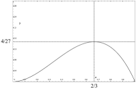
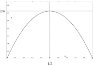
Figure 5: Maximizing $(1-r)r^{2}$ and $s(1-s)$

In order to do so, we first maximize $c_{1}c_{2}c_{3}$ under the constraints $c_{1},c_{2},c_{3}\geq 0$ and $c_{1}+c_{2}+c_{3}\leq 2$. Rewrite $c_{1}$ as $d(1-r)$, $c_{2}$ as $dr(1-s)$, and $c_{3}$ as $drs$, where $d\leq 2$ and $r,s\in[0,1]$. (Namely, let $d\mathrel{\buildrel\text{def}\over{=}}c_{1}+c_{2}+c_{3}$; if $d=0$, let $r$ and $s$ be arbitrary; otherwise, let $r\mathrel{\buildrel\text{def}\over{=}}1-c_{1}/d$; if $r=0$, then let $s$ be arbitrary; otherwise, let $s\mathrel{\buildrel\text{def}\over{=}}c_{3}/(dr)$.) The maximal value of $c_{1}c_{2}c_{3}=d^{3}(1-r)r^{2}s(1-s)$ is obtained by maximizing:

• $d$ (as $2$),

• $(1-r)r^{2}$ when $r\in[0,1]$ (value $4/27$ obtained at $r\mathrel{\buildrel\text{def}\over{=}}2/3$, see Figure 5, left),

• and $s(1-s)$ when $s\in[0,1]$ (value $1/4$ obtained at $s\mathrel{\buildrel\text{def}\over{=}}1/2$, see Figure 5, right),

hence is equal to $2\cdot(4/27)\cdot(1/4)=8/27$. It follows that for all $a_{1},b_{1},a_{2},b_{2},a_{3},b_{3}\in[0,1]$ such that $a_{1}+b_{1}+a_{2}+b_{2}+a_{3}+b_{3}\leq 2$, $b_{1}a_{2}a_{3}\leq(a_{1}+b_{1})(a_{2}+b_{2})(a_{3}+b_{3})\leq 8/27$, by taking $c_{i}\mathrel{\buildrel\text{def}\over{=}}a_{i}+b_{i}$ for each $i$. $\Box$

We sum up our results as follows. Note that $\mathop{\text{Pr}}[\mathtt{portest}\;P\mathbin{\downarrow}n]=0$, for any $P$, if $n\neq 0$.

Theorem 6.3

For every ground PCF_P term $P\colon D\mathtt{int}\to D\mathtt{int}\to D\mathtt{int}$, the probability $\mathop{\text{Pr}}[\mathtt{portest}\;P\mathbin{\downarrow}0]$ that $P$ fools the parallel or tester never exceeds $8/27$. That bound is attained by taking $P\mathrel{\buildrel\text{def}\over{=}}\mathtt{pmpor}$. $\Box$

7 Conclusion and Related Work

There is an extensive literature on the semantics of higher-order functional languages, and extensions that include probabilistic choice are now attracting attention more than ever.

Concerning denotational semantics, we should cite the following. Probabilistic coherence spaces provide a fully abstract semantics for a version of PCF with probabilistic choice, as shown by Ehrhard, Tasson, and Pagani [ETP14]. Quasi-Borel spaces and predomains have recently been used to give adequate semantics to typed and untyped probabilistic programming languages, see e.g. [VKS19]. QCB spaces form a convenient category in which various effects, including probabilistic choice, can be modeled [Bat06]. Comparatively, the domain-theoretic semantics we are using in this paper is rather mundane, and I have used similar models for further extensions that also include angelic [Gou15] and demonic [Gou19b] non-deterministic choice. In those papers, I obtain full abstraction at the price of adding some extra primitives, but also of considering a richer semantics that also includes forms of non-deterministic choice. The latter allows us to work in categories with nice properties. That is not available in the context of PCF_P, because there is no known Cartesian-closed category of continuous dcpos that is closed under $\mathbf{V}_{\leq 1}$ [JT98].

Let me remind the reader that denotational semantics is only a tool here: the result we have presented concerns the operational semantics, and domain-theory is only used, through adequacy, in order to bound $\mathop{\text{Pr}}[\mathtt{portest}\;P\mathbin{\downarrow}*]$. One may wonder whether a direct operational approach would work, but I doubt it strongly. Eventually, any operational approach would have to find suitable invariants, and such invariants will be hard to distinguish from an actual denotational semantics.

One may wonder whether such semantical proofs would be useful in the realm of probabilistic process algebras as well. In non-probabilistic process algebras, syntactic reasoning is usually enough, using bisimulations and up-to techniques. The case of probabilistic processes is necessarily more complex, and may benefit from such semantical arguments.

Appendix A Soundness

There is a unique way of defining a denotational semantics $\left\llbracket{C}\right\rrbracket\rho$ of contexts $C$ in such a way that $\left\llbracket{C[M]}\right\rrbracket\rho=\left\llbracket{C}\right\rrbracket\rho(\left\llbracket{M}\right\rrbracket\rho)$ for every $M$ of the right type and every $\rho\in Env$. For $C\mathrel{\buildrel\text{def}\over{=}}E_{0}E_{1}\cdots E_{n}$, $\left\llbracket{C}\right\rrbracket\rho$ is the composition of the maps $\left\llbracket{E_{0}}\right\rrbracket\rho$, $\left\llbracket{E_{1}}\right\rrbracket\rho$, …, $\left\llbracket{E_{n}}\right\rrbracket\rho$, where for each elementary or initial context $E$, $\left\llbracket{E}\right\rrbracket\rho$ is defined by:

• for every $N\colon\sigma$, $\left\llbracket{[\_N]}\right\rrbracket\rho(f)\mathrel{\buildrel\text{def}\over{=}}f(\left\llbracket{N}\right\rrbracket\rho)$;

• $\left\llbracket{[{\mathtt{p}}\_]}\right\rrbracket\rho(n)\mathrel{\buildrel\text{def}\over{=}}n-1$, $\left\llbracket{[{\mathtt{s}}\_]}\right\rrbracket\rho(n)\mathrel{\buildrel\text{def}\over{=}}n+1$;

• $\left\llbracket{[\mathop{\mathtt{if}}\nolimits{\_}=0\;\mathtt{then}\;{N}\;\mathbin{\mathtt{else}}{P}]}\right\rrbracket\rho(n)\mathrel{\buildrel\text{def}\over{=}}\left\llbracket{N}\right\rrbracket\rho$ if $n=0$, $\left\llbracket{P}\right\rrbracket\rho$ otherwise;

• $\left\llbracket{[\mathop{\mathtt{bind}}\nolimits_{\sigma,\tau}\_N]}\right\rrbracket\rho\mathrel{\buildrel\text{def}\over{=}}(\left\llbracket{N}\right\rrbracket\rho)^{\dagger}$;

• $\left\llbracket{[\mathop{\mathtt{ret}}\nolimits_{\mathtt{int}}\_]}\right\rrbracket\rho(n)\mathrel{\buildrel\text{def}\over{=}}\eta(n)=\delta_{n}$;

• $\left\llbracket{[\_]}\right\rrbracket\rho(\nu)\mathrel{\buildrel\text{def}\over{=}}\nu$;

It is standard that $\left\llbracket{M}\right\rrbracket\rho$ only depends on the value of $\rho$ on the free variables of $M$ (if $\rho(x)=\rho^{\prime}(x)$ for every free variable $x$ of $M$, then $\left\llbracket{M}\right\rrbracket\rho=\left\llbracket{M}\right\rrbracket\rho^{\prime}$), and that for every substitution $\theta\mathrel{\buildrel\text{def}\over{=}}[x_{1}:=N_{1},\cdots,x_{n}:=N_{n}]$, $\left\llbracket{M\theta}\right\rrbracket\rho=\left\llbracket{M}\right\rrbracket(\left\llbracket{\theta}\right\rrbracket\rho)$, where $\left\llbracket{\theta}\right\rrbracket\rho$ is the environment that maps every $x_{i}$, $1\leq i\leq n$, to $\left\llbracket{N_{i}}\right\rrbracket\rho$ and all other variables $y$ to $\rho(y)$. In particular, $\left\llbracket{M[x_{\sigma}:=N]}\right\rrbracket\rho=\left\llbracket{M}\right\rrbracket(\rho[x_{\sigma}\mapsto\left\llbracket{N}\right\rrbracket\rho])$. Finally, $\left\llbracket{(\lambda x_{\sigma}.M)N}\right\rrbracket\rho$ is equal to $\left\llbracket{M[x_{\sigma}:=N]}\right\rrbracket\rho$. We have:

Lemma A.1

Let $\rho$ be an environment.

1. For every rule of the form $s\mathrel{\buildrel 1\over{\to}}t$, $\left\llbracket{s}\right\rrbracket\rho=\left\llbracket{t}\right\rrbracket\rho$.

2. For every context $C$ of type $D\sigma\vdash D\mathtt{int}$, for all $M,N\colon D\sigma$, $\left\llbracket{C\cdot M\oplus N}\right\rrbracket\rho=\frac{1}{2}\left\llbracket{C\cdot M}\right\rrbracket\rho+\frac{1}{2}\left\llbracket{C\cdot N}\right\rrbracket\rho$.

Proof. 1. All the cases are easily checked, except perhaps for the rule $C[\mathop{\mathtt{bind}}\nolimits_{\sigma,\tau}\_N]\cdot\mathop{\mathtt{ret}}\nolimits_{\sigma}M\mathrel{\buildrel 1\over{\to}}C\cdot NM$. That reduces to showing the equality $\left\llbracket{\mathop{\mathtt{bind}}\nolimits_{\sigma,\tau}(\mathop{\mathtt{ret}}\nolimits_{\sigma}M)N}\right\rrbracket\rho=\left\llbracket{NM}\right\rrbracket\rho$. The left-hand side is $(\left\llbracket{N}\right\rrbracket\rho)^{\dagger}(\eta(\left\llbracket{M}\right\rrbracket\rho))$, which is equal to $\left\llbracket{N}\right\rrbracket\rho(\left\llbracket{M}\right\rrbracket\rho)$, by (1). In turn, that is $\left\llbracket{NM}\right\rrbracket\rho$.

2. Let $C\mathrel{\buildrel\text{def}\over{=}}E_{0}E_{1}\cdots E_{n}$. By inspection of types, all the elementary contexts $E_{i}$, $1\leq i\leq n$, must be of the form $[\mathop{\mathtt{bind}}\nolimits_{\sigma_{i+1},\sigma_{i}}\_N_{i}]$ for some $N_{i}\colon\sigma_{i+1}\to D\sigma_{i}$, $E_{0}=[\_]$, and $\sigma_{1}=\mathtt{int}$.

We observe that $\left\llbracket{E_{i}}\right\rrbracket\rho=(\left\llbracket{N_{i}}\right\rrbracket\rho)^{\dagger}$ is a linear map. In fact, $f^{\dagger}$ is linear for every Scott-continuous map $f\colon X\to Y$, in the following sense: for all $a,b\in\mathbb{R}_{+}$ with $a+b\leq 1$, for all $\mu,\nu\in\mathbf{V}_{\leq 1}X$, $f^{\dagger}(a\mu+b\nu)=af^{\dagger}(\mu)+bf^{\dagger}(\nu)$. Indeed, for every $V\in\mathcal{O}Y$, $f^{\dagger}(a\mu+b\nu)(V)=\int_{x\in X}f(x)(V)d(a\mu+b\nu)=a\int_{x\in X}f(x)(V)d\mu+b\int_{x\in X}f(x)(V)d\nu=af^{\dagger}(\mu)(V)+bf^{\dagger}(\nu)(V)$.

It follows that $\left\llbracket{C}\right\rrbracket\rho$ is also a linear map. Then $\left\llbracket{C\cdot M\oplus N}\right\rrbracket\rho=\left\llbracket{C}\right\rrbracket\rho(\frac{1}{2}\left\llbracket{M}\right\rrbracket\rho+\frac{1}{2}\left\llbracket{N}\right\rrbracket\rho)=\frac{1}{2}\left\llbracket{C}\right\rrbracket\rho(\left\llbracket{M}\right\rrbracket\rho)+\frac{1}{2}\left\llbracket{C}\right\rrbracket(\left\llbracket{N}\right\rrbracket\rho)=\frac{1}{2}\left\llbracket{C\cdot M}\right\rrbracket\rho+\frac{1}{2}\left\llbracket{C\cdot N}\right\rrbracket\rho$. $\Box$

Proposition A.2 (Soundness)

For every configuration $s$ of type $D\mathtt{int}$, for every $n\in\mathbb{Z}$, for every environment $\rho$, $\left\llbracket{s}\right\rrbracket\rho(\{n\})\geq\mathop{\text{Pr}}[s\mathbin{\downarrow}n]$.

Proof. It suffices to show that for every $r\in\mathbb{R}_{+}$ such that $r<\mathop{\text{Pr}}[s\mathbin{\downarrow}n]$, $r\leq\left\llbracket{s}\right\rrbracket\rho(\{n\})$. We write $\mathop{\text{Pr}}[s\mathbin{\downarrow}V]$ as a possibly infinite sum. Since $r<\mathop{\text{Pr}}[s\mathbin{\downarrow}n]$, there is a finite subset of the summands which sum to at least $r$. In other words, there is a finite set of traces starting at $s$ and ending at $[\mathop{\mathtt{ret}}\nolimits_{\mathtt{int}}\_]\cdot n$, whose weights sum up to at least $r$. Let $N$ be some upper bound on the lengths of those traces. By induction on $N$, we show that the sum $\mathop{\text{Pr}}_{\leq N}[s\mathbin{\downarrow}n]$ of all weights of traces of length at most $N$, starting at $s$ and ending at $[\mathop{\mathtt{ret}}\nolimits_{\mathtt{int}}\_]\cdot n$, is less than or equal to $\left\llbracket{s}\right\rrbracket\rho(\{n\})$, and this will prove the claim.

If $s=[\mathop{\mathtt{ret}}\nolimits_{\mathtt{int}}\_]\cdot n$, then $\left\llbracket{s}\right\rrbracket\rho(\{n\})=\delta_{\left\llbracket{n}\right\rrbracket\rho}(\{n\})=1$. Therefore $\mathop{\text{Pr}}_{\leq N}[s\mathbin{\downarrow}n]\leq\left\llbracket{s}\right\rrbracket\rho(\{n\})$.

From now on, we assume that $s$ is not of the form $[\mathop{\mathtt{ret}}\nolimits_{\mathtt{int}}\_]\cdot n$.

If $N=0$, then there is no trace of length at most $N$ starting at $s$ and ending at $[\mathop{\mathtt{ret}}\nolimits_{\mathtt{int}}\_]\cdot n$, so $\mathop{\text{Pr}}_{\leq N}[s\mathbin{\downarrow}n]=0\leq\left\llbracket{s}\right\rrbracket\rho(\{n\})$.

If $N\geq 1$, then we explore three cases.

If no rule applies to $s$, namely if $s\mathrel{\buildrel a\over{\to}}t$ for no $a$ and no $t$, then $\mathop{\text{Pr}}_{\leq N}[s\mathbin{\downarrow}n]=0\leq\left\llbracket{s}\right\rrbracket\rho(\{n\})$.

If $s$ if of the form $C\cdot M\oplus N$ then $\mathop{\text{Pr}}_{\leq N-1}(C\cdot M\mathbin{\downarrow}n)\leq\left\llbracket{C\cdot M}\right\rrbracket\rho(\{n\})$ and $\mathop{\text{Pr}}_{\leq N-1}(C\cdot N\mathbin{\downarrow}n)\leq\left\llbracket{C\cdot N}\right\rrbracket\rho(\{n\})$, by induction hypothesis. Now $\mathop{\text{Pr}}_{\leq N}(s\mathbin{\downarrow}n)=\frac{1}{2}\mathop{\text{Pr}}_{\leq N-1}(C\cdot M\mathbin{\downarrow}n)+\frac{1}{2}\mathop{\text{Pr}}_{\leq N-1}(C\cdot N\mathbin{\downarrow}n)$, which is less than or equal to $\frac{1}{2}\left\llbracket{C\cdot M}\right\rrbracket\rho(\{n\})+\frac{1}{2}\left\llbracket{C\cdot N}\right\rrbracket\rho(\{n\})=\left\llbracket{C\cdot M\oplus N}\right\rrbracket\rho(\{n\})$, by Lemma A.1, item 2.

In all other cases, $s\mathrel{\buildrel 1\over{\to}}t$ for some unique configuration $t$, so that $\mathop{\text{Pr}}_{\leq N}(s\mathbin{\downarrow}n)=\mathop{\text{Pr}}_{\leq N-1}(t\mathbin{\downarrow}n)\leq\left\llbracket{t}\right\rrbracket\rho(\{n\})$, by induction hypothesis. By Lemma A.1, item 1, the latter is equal to $\left\llbracket{s}\right\rrbracket\rho(\{n\})$. $\Box$

Appendix B Adequacy

The key to proving the converse of soundness is the design of a suitable logical relation $\mathrel{R}\mathrel{\buildrel\text{def}\over{=}}{(\mathrel{R}_{\tau})}_{\tau\text{ type}}$, where each $\mathrel{R}_{\tau}$ is a binary relation between ground terms $M$ of type $\tau$ and elements of $\left\llbracket{\tau}\right\rrbracket$. Since $\left\llbracket{M}\right\rrbracket\rho$ does not depend on $\rho$ when $M$ is ground, we simply write $\left\llbracket{M}\right\rrbracket$ in that case. We write $\left\llbracket{C}\right\rrbracket$ similarly for ground contexts $C$.

The definition of $\mathrel{R}_{\tau}$ is by induction on $\tau$, using auxiliary relations $\mathrel{R}_{D\tau}^{\perp}$ between ground contexts $C\colon D\tau\to D\mathtt{int}$ and Scott-continuous maps $h\colon\left\llbracket{D\tau}\right\rrbracket\to\left\llbracket{D\mathtt{int}}\right\rrbracket$:

• for all ground $M\colon\mathtt{int}$ and $n\in\mathbb{Z}$, $M\mathrel{R}_{\mathtt{int}}n$ if and only if $[\_]\cdot M\mathrel{\buildrel 1\over{\to}{}^{*}}[\_]\cdot n$;

• for all types $\sigma$, $\tau$, for all ground $M\colon\sigma\to\tau$ and $f\in\left\llbracket{\sigma\to\tau}\right\rrbracket$, $M\mathrel{R}_{\sigma\to\tau}f$ if and only if for all $N\mathrel{R}_{\sigma}a$, $MN\mathrel{R}_{\tau}f(a)$ (we say “for all $N\mathrel{R}_{\sigma}a$” instead of “for every ground $N\colon\sigma$ and for every $a\in\left\llbracket{\sigma}\right\rrbracket$ such that $N\mathrel{R}_{\sigma}a$”);

• for every type $\tau$, for all ground $M\colon D\tau$ and $\nu\in\left\llbracket{D\tau}\right\rrbracket$, $M\mathrel{R}_{D\tau}\nu$ if and only if for every ground context $C\colon D\tau\vdash D\mathtt{int}$, for every Scott-continuous map $h\colon\left\llbracket{D\tau}\right\rrbracket\to\left\llbracket{D\mathtt{int}}\right\rrbracket$ such that $C\mathrel{R}_{D\tau}^{\perp}h$, for every $n\in\mathbb{Z}$, $\mathop{\text{Pr}}[C\cdot M\mathbin{\downarrow}n]\geq h(\nu)(\{n\})$;

• for every type $\tau$, for every ground context $C\colon D\tau\vdash D\mathtt{int}$, for every Scott-continuous map $h\colon\left\llbracket{D\tau}\right\rrbracket\to\left\llbracket{D\mathtt{int}}\right\rrbracket$, $C\mathrel{R}_{D\tau}^{\perp}h$ if and only if for all $P\mathrel{R}_{\tau}a$, for every $n\in\mathbb{Z}$, $\mathop{\text{Pr}}[C\cdot\mathop{\mathtt{ret}}\nolimits_{\tau}P\mathbin{\downarrow}n]\geq h(\eta(a))(\{n\})$.

Lemma B.1

If $C\cdot M\mathrel{\buildrel 1\over{\to}{}^{*}}C\cdot N$ by any sequence of rules except the rule $[\_]\cdot\mathop{\mathtt{ret}}\nolimits_{\mathtt{int}}P\mathrel{\buildrel 1\over{\to}}[\mathop{\mathtt{ret}}\nolimits_{\mathtt{int}}\_]\cdot P$, then for every context $C^{\prime}$ of the expected type, $C^{\prime}C\cdot M\mathrel{\buildrel 1\over{\to}{}^{*}}C^{\prime}C\cdot N$.

Proof. It suffices to show the claim under the assumption that $C\cdot M\mathrel{\buildrel 1\over{\to}}C\cdot N$ by any other rule than the one we excluded. This is clear, since no rule except the one we excluded requires the context to have any specific shape. $\Box$

Lemma B.2

For every context $C\colon\sigma\vdash\tau$, for every term $M\colon\sigma$,

1. $[\_]\cdot C[M]\mathrel{\buildrel 1\over{\to}{}^{*}}C\cdot M$ by using the exploration rules only;

2. the run starting at $[\_]\cdot C[M]$ must start with the trace $[\_]\cdot C[M]\mathrel{\buildrel 1\over{\to}{}^{*}}C\cdot M$, followed by the run starting at $C\cdot M$.

Proof. 1 is clear. 2 is because the operational semantics is deterministic, in the sense that $s\mathrel{\buildrel 1\over{\to}}t_{0}$ and $s\mathrel{\buildrel 1\over{\to}}t_{1}$ implies $t_{0}=t_{1}$. $\Box$

Lemma B.3

For every context $C\colon\sigma\vdash\tau$, if $\sigma$ is a computation type, then so is $\tau$.

Proof. By inspection of the elementary contexts.

Lemma B.4

For every configuration $s$ of type $\mathtt{int}$, every trace $s\mathrel{\buildrel\alpha\over{\to}{}^{*}}s^{\prime}$ satisfies $\alpha=1$. Moreover, it does not use the rule $[\_]\cdot\mathop{\mathtt{ret}}\nolimits_{\beta}P\mathrel{\buildrel 1\over{\to}}[\mathop{\mathtt{ret}}\nolimits_{\beta}\_]\cdot P$.

Proof. It is enough to show the claim under the assumption that $s\mathrel{\buildrel\alpha\over{\to}}s^{\prime}$. Let us write $s$ as $C\cdot M$, where $C$ is of type $\sigma\vdash\beta$ and $M\colon\sigma$. By Lemma B.3, $\sigma$ cannot be a computation type. It follows that the rule that was used cannot be $C\cdot P\oplus Q\mathrel{\buildrel 1/2\over{\to}}C\cdot P$ or $C\cdot P\oplus Q\mathrel{\buildrel 1/2\over{\to}}C\cdot Q$, since $P\oplus Q$ has a computation type. Similarly, it cannot be $[\_]\cdot\mathop{\mathtt{ret}}\nolimits_{\beta}P\mathrel{\buildrel 1\over{\to}}[\mathop{\mathtt{ret}}\nolimits_{\beta}\_]\cdot P$, again because $\mathop{\mathtt{ret}}\nolimits_{\beta}P$ has a computation type.

Lemma B.5

For all terms $M\colon\tau$ and $N\colon\sigma$, for every context $C^{\prime}\colon\sigma\vdash\tau$, for every $V\in\left\llbracket{\tau}\right\rrbracket$, if $[\_]\cdot M\mathrel{\buildrel 1\over{\to}{}^{*}}C^{\prime}\cdot N$ without using the rule $[\_]\cdot\mathop{\mathtt{ret}}\nolimits_{\mathtt{int}}P\mathrel{\buildrel 1\over{\to}}[\mathop{\mathtt{ret}}\nolimits_{\mathtt{int}}\_]\cdot P$, and if $C^{\prime}[N]\mathrel{R}_{\tau}V$, then $M\mathrel{R}_{\tau}V$.

Proof. By induction on $\tau$. If $\tau=\mathtt{int}$, $C^{\prime}[N]\mathrel{R}_{\tau}V$ means that $[\_]\cdot C^{\prime}[N]\mathrel{\buildrel 1\over{\to}{}^{*}}[\_]\cdot V$. By Lemma B.2, item 2, our trace starting at $[\_]\cdot C^{\prime}[N]$ and ending at $[\_]\cdot V$ must factor as $[\_]\cdot C^{\prime}[N]\mathrel{\buildrel 1\over{\to}{}^{*}}C^{\prime}\cdot N\mathrel{\buildrel 1\over{\to}{}^{*}}[\_]\cdot V$. Hence $[\_]\cdot M\mathrel{\buildrel 1\over{\to}{}^{*}}C^{\prime}\cdot N\mathrel{\buildrel 1\over{\to}{}^{*}}[\_]\cdot V$, showing that $M\mathrel{R}_{\tau}V$.

For types of the form $D\tau$, our task is to show that $M\mathrel{R}_{D\tau}\nu$, where $\nu$ is any subprobability valuation in $\left\llbracket{D\tau}\right\rrbracket$, knowing that $C^{\prime}[N]\mathrel{R}_{\tau}\nu$. We let $C\colon D\tau\vdash D\mathtt{int}$ be an arbitrary ground context, $h\colon\left\llbracket{D\tau}\right\rrbracket\to\left\llbracket{D\mathtt{int}}\right\rrbracket$ be an arbitrary Scott-continuous map such that $C\mathrel{R}_{D\tau}^{\perp}h$, and we wish to show that for every $n\in\left\llbracket{\mathtt{int}}\right\rrbracket$, $\mathop{\text{Pr}}[C\cdot M\mathbin{\downarrow}n]\geq h(\nu)(\{n\})$. By Lemma B.1, $C\cdot M\mathrel{\buildrel 1\over{\to}{}^{*}}CC^{\prime}\cdot N$. Since $C^{\prime}[N]\mathrel{R}_{\tau}\nu$, $\mathop{\text{Pr}}[C\cdot C^{\prime}[N]\mathbin{\downarrow}n]\geq h(\nu)(\{n\})$. By Lemma B.2, item 2, the run starting at $C\cdot C^{\prime}[N]$ must factor as a trace $C\cdot C^{\prime}[N]\mathrel{\buildrel 1\over{\to}{}^{*}}CC^{\prime}\cdot N$ followed by a run starting at $CC^{\prime}\cdot N$, so $\mathop{\text{Pr}}[C\cdot C^{\prime}[N]\mathbin{\downarrow}n]=\mathop{\text{Pr}}[CC^{\prime}\cdot N\mathbin{\downarrow}n]$. Prepending instead the trace $C\cdot M\mathrel{\buildrel 1\over{\to}{}^{*}}CC^{\prime}\cdot N$ (i.e., using Lemma 3.3, item 2), we see that $\mathop{\text{Pr}}[C\cdot M\mathbin{\downarrow}n]=\mathop{\text{Pr}}[CC^{\prime}\cdot N\mathbin{\downarrow}n]$. That is equal to $\mathop{\text{Pr}}[C\cdot C^{\prime}[N]\mathbin{\downarrow}n]$, which is larger than or equal to $h(\nu)(\{n\})$ since $C^{\prime}[N]\mathrel{R}_{\tau}\nu$ and $C\mathrel{R}_{D\tau}^{\beta\perp}h$.

For function types $\sigma\to\tau$, we wish to show that $M\mathrel{R}_{\sigma\to\tau}f$, where $f\in\left\llbracket{\sigma\to\tau}\right\rrbracket$, knowing that $C^{\prime}[N]\mathrel{R}_{\sigma\to\tau}f$. The latter means that for all $P\mathrel{R}_{\sigma}a$, $C^{\prime}[N]P\mathrel{R}_{\tau}f(a)$. For every $C$, there is a trace $C\cdot MP\mathrel{\buildrel 1\over{\to}}C[\_P]\cdot M\mathrel{\buildrel 1\over{\to}{}^{*}}C[\_P]C^{\prime}\cdot N$, by Lemma B.1 with context $C[\_P]$, and this trace does not use the rule $[\_]\cdot\mathop{\mathtt{ret}}\nolimits_{\beta}Q\mathrel{\buildrel 1\over{\to}}[\mathop{\mathtt{ret}}\nolimits_{\beta}\_]\cdot Q$. By induction hypothesis (using $[\_P]C^{\prime}$ instead of $C^{\prime}$), $MP\mathrel{R}_{\tau}f(b)$. Since $P$ and $b$ are arbitrary, $M\mathrel{R}_{\sigma\to\tau}f$. $\Box$

By taking $C^{\prime}\mathrel{\buildrel\text{def}\over{=}}[\_]$, we obtain the following.

Corollary B.6

Let $M,N\colon\tau$, and $V\in\left\llbracket{\tau}\right\rrbracket$. If $[\_]\cdot M\mathrel{\buildrel 1\over{\to}{}^{*}}[\_]\cdot N$ by any sequence of rules except $[\_]\cdot\mathop{\mathtt{ret}}\nolimits_{\mathtt{int}}P\mathrel{\buildrel 1\over{\to}}[\mathop{\mathtt{ret}}\nolimits_{\mathtt{int}}\_]\cdot P$, and if $N\mathrel{R}_{\tau}V$ then $M\mathrel{R}_{\tau}V$. $\Box$

Lemma B.7

For every ground term $M\colon\tau$, the set $M\mathrel{R}_{\tau}$, defined as the set of elements $a\in\left\llbracket{\tau}\right\rrbracket$ such that $M\mathrel{R}_{\tau}a$, is Scott-closed. If $\tau$ is a computation type, then it also contains the least element $\bot_{\tau}$ of $\left\llbracket{\tau}\right\rrbracket$.

Proof. By induction on $\tau$. When $\tau=\mathtt{int}$, this is obvious. Let us consider the case of types of the form $D\tau$. For every ground context $C\colon D\tau\vdash D\mathtt{int}$, for every Scott-continuous map $h\colon\left\llbracket{D\tau}\right\rrbracket\to\left\llbracket{D\mathtt{int}}\right\rrbracket$ such that $C\mathrel{R}_{D\tau}^{\perp}h$, for every $n\in\left\llbracket{\mathtt{int}}\right\rrbracket$, the set $\Gamma_{C,h,n}\mathrel{\buildrel\text{def}\over{=}}\{\nu\in\left\llbracket{D\tau}\right\rrbracket\mid h(\nu)(\{n\})\leq\mathop{\text{Pr}}[C\cdot M\mathbin{\downarrow}n]\}$ is Scott-closed: it is easily seen to be downwards-closed, and for every directed family ${(\nu_{i})}_{i\in I}$ in $\Gamma_{C,h,n}$, $h(\sideset{}{{}^{\,\makebox[0.0pt]{$\scriptstyle\uparrow$}\!}}{\sup}_{i\in I}\nu_{i})(\{n\})=\sideset{}{{}^{\,\makebox[0.0pt]{$\scriptstyle\uparrow$}\!}}{\sup}_{i\in I}h(\nu_{i})(\{n\})\leq\mathop{\text{Pr}}[C\cdot M\mathbin{\downarrow}n]$, so $\sideset{}{{}^{\,\makebox[0.0pt]{$\scriptstyle\uparrow$}\!}}{\sup}_{i\in I}\nu_{i}\in\Gamma_{C,h,n}$. $M\mathrel{R}_{D\tau}$ is the intersection of all the sets $\Gamma_{C,h,n}$, hence is Scott-closed as well. It also contains the least element of $\left\llbracket{D\mathtt{int}}\right\rrbracket$, the zero valuation, since $\mathop{\text{Pr}}[C\cdot M\mathbin{\downarrow}n]\geq 0$ for all $C$ and $n$.

Finally, we consider function types. Let $M\colon\sigma\to\tau$ be ground, and let us show that $M\mathrel{R}_{\sigma\to\tau}$ is Scott-closed. That is equal to the intersection over all $N\mathrel{R}_{\sigma}a$ of the sets $\Delta_{N,a}$, where $\Delta_{N,a}\mathrel{\buildrel\text{def}\over{=}}\{f\in\left\llbracket{\sigma\to\tau}\right\rrbracket\mid f(a)\in(MN\mathrel{R}_{\tau})\}$. $\Delta_{N,a}$ is clearly downwards-closed; for Scott closure, for every directed family ${(f_{i})}_{i\in I}$ in $\Delta_{N,a}$, $(\sideset{}{{}^{\,\makebox[0.0pt]{$\scriptstyle\uparrow$}\!}}{\sup}_{i\in I}f_{i})(a)=\sideset{}{{}^{\,\makebox[0.0pt]{$\scriptstyle\uparrow$}\!}}{\sup}_{i\in I}f_{i}(a)$ is in $MN\mathrel{R}_{\tau}$, because the latter is Scott-closed by induction hypothesis. Taking intersections, $M\mathrel{R}_{\sigma\to\tau}$ is Scott-closed as well.

When $\sigma\to\tau$ is a computation type, $\tau$ is one, too, and by induction hypothesis $MN\mathrel{R}_{\tau}\bot_{\tau}$ for all $N\mathrel{R}_{\sigma}a$. That means that $MN\mathrel{R}_{\tau}\bot_{\sigma\to\tau}(a)$ for all $N\mathrel{R}_{\sigma}a$, hence that $M\mathrel{R}_{\sigma\to\tau}\bot_{\sigma\to\tau}$.

Corollary B.8

For every computation type $\tau$, for all $M\mathrel{R}_{\tau\to\tau}f$, $\mathop{\mathtt{rec}}\nolimits_{\tau}M\mathrel{R}_{\tau}\mathop{\mathrm{lfp}}\nolimits_{\left\llbracket{\tau}\right\rrbracket}f$.

Proof. By the second part of Lemma B.7, $\mathop{\mathtt{rec}}\nolimits_{\tau}M\theta\mathrel{R}_{\tau}\bot_{\tau}$.

Additionally, for every $a\in\left\llbracket{\tau}\right\rrbracket$, if $\mathop{\mathtt{rec}}\nolimits_{\tau}M\mathrel{R}_{\tau}a$ then $M(\mathop{\mathtt{rec}}\nolimits_{\tau}M)\mathrel{R}_{\tau}f(a)$, since $M\mathrel{R}_{\tau\to\tau}f$. Using Corollary B.6 with the step $[\_]\cdot\mathop{\mathtt{rec}}\nolimits_{\tau}M\mathrel{\buildrel 1\over{\to}}M(\mathop{\mathtt{rec}}\nolimits_{\tau}M)$, it follows that $\mathop{\mathtt{rec}}\nolimits_{\tau}M\mathrel{R}_{\tau}f(a)$.

Hence for every $a\in\mathop{\mathtt{rec}}\nolimits_{\tau}M\mathrel{R}_{\tau}$, $f(a)$ is also in $\mathop{\mathtt{rec}}\nolimits_{\tau}M\mathrel{R}_{\tau}$. It follows that $f^{n}(\bot_{\tau})$ is in $\mathop{\mathtt{rec}}\nolimits_{\tau}M\mathrel{R}_{\tau}$ for every $n\in\mathbb{N}$. By Lemma B.7, $\sideset{}{{}^{\,\makebox[0.0pt]{$\scriptstyle\uparrow$}\!}}{\sup}_{n\in\mathbb{N}}f^{n}(\bot_{\tau})$ must also be in $\mathop{\mathtt{rec}}\nolimits_{\tau}M\mathrel{R}_{\tau}$, and that is just $\mathop{\mathrm{lfp}}\nolimits_{\left\llbracket{\tau}\right\rrbracket}(f)$. $\Box$

Lemma B.9

Let $\sigma$ be a type. For all $M\mathrel{R}_{\sigma}a$, $\mathop{\mathtt{ret}}\nolimits_{\sigma}M\mathrel{R}_{D\sigma}\eta(a)$.

Proof. Relying on the definition of $\mathrel{R}_{D\sigma}$, let $\beta$ be a basic type, $C\colon D\sigma\vdash D\beta$ be a ground context, $h\colon\left\llbracket{D\sigma}\right\rrbracket\to\left\llbracket{D\beta}\right\rrbracket$ be Scott-continuous, and assume that $C\mathrel{R}_{D\sigma}^{\beta\perp}h$. By definition of $\mathrel{R}_{D\sigma}^{\beta\perp}$, and since $M\mathrel{R}_{\sigma}a$, we obtain $\mathop{\text{Pr}}[C\cdot\mathop{\mathtt{ret}}\nolimits_{\sigma}M\mathbin{\downarrow}V]\geq h(\eta(a))$, and that is what we wanted to show.

Lemma B.10

Let $\sigma$, $\tau$ be types. For all $M\mathrel{R}_{D\sigma}\nu$ and $N\mathrel{R}_{\sigma\to D\tau}f$, we have $\mathop{\mathtt{bind}}\nolimits_{\sigma,\tau}MN\mathrel{R}_{D\tau}f^{\dagger}(\nu)$.

Proof. We plan to use the definition of $\mathrel{R}_{D\tau}$, and for that we fix an arbitrary ground context $C\colon D\tau\vdash D\mathtt{int}$, an arbitrary Scott-continuous map $h\colon\left\llbracket{D\tau}\right\rrbracket\to\left\llbracket{D\mathtt{int}}\right\rrbracket$ such that $C\mathrel{R}_{D\tau}^{\perp}h$, and we wish to show: $(*)$ for every $n\in\mathbb{Z}$, $\mathop{\text{Pr}}[C\cdot\mathop{\mathtt{bind}}\nolimits_{\sigma,\tau}MN\mathbin{\downarrow}n]\geq h(f^{\dagger}(\nu))(\{n\})$.

For all $P\mathrel{R}_{\sigma}a$, by definition of $\mathrel{R}_{\sigma\to D\tau}$, we have $NP\mathrel{R}_{D\tau}f(a)$. Since $C\mathrel{R}_{D\tau}^{\perp}h$, and using the definition of $R_{D\tau}$, we obtain that $\mathop{\text{Pr}}[C\cdot NP\mathbin{\downarrow}n]\geq h(f(a))(\{n\})$ for every $n\in\mathbb{Z}$. We note that $C[\mathop{\mathtt{bind}}\nolimits_{\sigma,\tau}\_N]\cdot\mathop{\mathtt{ret}}\nolimits_{\sigma}P\mathrel{\buildrel 1\over{\to}}C\cdot NP$ and we use Lemma 3.3, item 2, so $\mathop{\text{Pr}}[C[\mathop{\mathtt{bind}}\nolimits_{\sigma,\tau}\_N]\cdot\mathop{\mathtt{ret}}\nolimits_{\sigma}P\mathbin{\downarrow}n]\geq h(f(a))(\{n\})$. By (1), $f=f^{\dagger}\circ\eta$, so $\mathop{\text{Pr}}[C[\mathop{\mathtt{bind}}\nolimits_{\sigma,\tau}\_N]\cdot\mathop{\mathtt{ret}}\nolimits_{\sigma}P\mathbin{\downarrow}n]\geq h(f^{\dagger}(\eta(a)))(\{n\})$. Since $n$, $P$ and $a$ are arbitrary such that $P\mathrel{R}_{\sigma}a$, we obtain that $C[\mathop{\mathtt{bind}}\nolimits_{\sigma,\tau}\_N]\mathrel{R}_{D\sigma}^{\perp}h\circ f^{\dagger}$, by definition of $\mathrel{R}_{D\sigma}^{\perp}$.

From that and $M\mathrel{R}_{D\sigma}\nu$, it follows that, for every $n\in\mathbb{Z}$, $\mathop{\text{Pr}}[C[\mathop{\mathtt{bind}}\nolimits_{\sigma,\tau}\_N]\cdot M\mathbin{\downarrow}n]\geq h(f^{\dagger}(\nu))(\{n\})$. Since $C\cdot\mathop{\mathtt{bind}}\nolimits_{\sigma,\tau}MN\mathrel{\buildrel 1\over{\to}}C[\mathop{\mathtt{bind}}\nolimits_{\sigma,\tau}\_N]\cdot M$, and using Lemma 3.3, item 2, we obtain $\mathop{\text{Pr}}[C\cdot\mathop{\mathtt{bind}}\nolimits_{\sigma,\tau}MN\mathbin{\downarrow}n]\geq h(f^{\dagger}(\nu))(\{n\})$. Since $n$, $C$ and $h$ are arbitrary such that $C\mathrel{R}_{D\tau}^{\mathtt{int}\perp}h$, $\mathop{\mathtt{bind}}\nolimits_{\sigma,\tau}MN\mathrel{R}_{D\sigma}f^{\dagger}(\nu)$. $\Box$

The crucial property of logical relations is the following basic lemma of logical relations. For a ground substitution $\theta\mathrel{\buildrel\text{def}\over{=}}[x_{1}:=N_{1},\cdots,x_{k}:=N_{k}]$ and an environment $\rho$, we write $\theta\mathrel{R}_{*}\rho$ to mean that for every $i$, $1\leq i\leq k$, $N_{i}\mathrel{R}_{\tau_{i}}\rho(x_{i})$, where $\tau_{i}$ is the type of $x_{i}$. The following is the basic lemma of logical relations for the case at hand.

Proposition B.11

For every PCF_P term $M\colon\tau$, for every ground substitution $\theta$ such that all the free variables of $M$ are in $\mathop{\mathrm{dom}}\theta$, and for every environment $\rho$ such that $\theta\mathrel{R}_{*}\rho$, $M\theta\mathrel{R}_{\tau}\left\llbracket{M}\right\rrbracket\rho$.

Proof. This is by induction on the structure of $M$. If $M=x_{i}$ for some $i$, $1\leq i\leq n$ (where $\theta=[x_{1}:=N_{1},\cdots,x_{n}:=N_{n}]$), then this follows from the assumption $\theta\mathrel{R}_{*}\rho$.

If $M$ is a constant $n\in\mathbb{Z}$, then $n\mathrel{R}_{\mathtt{int}}n$, because $[\_]\cdot n\mathrel{\buildrel 1\over{\to}{}^{*}}[\_]\cdot n$, trivially. If $M={\mathtt{s}}N$, then by induction hypothesis $N\theta\mathrel{R}_{\mathtt{int}}n$, where $n\mathrel{\buildrel\text{def}\over{=}}\left\llbracket{N}\right\rrbracket\rho$. Therefore $[\_]\cdot N\mathrel{\buildrel 1\over{\to}{}^{*}}[\_]\cdot n$. By Lemma B.4, that trace does not use the rule $[\_]\cdot\mathop{\mathtt{ret}}\nolimits_{\beta}P\mathrel{\buildrel 1\over{\to}}[\mathop{\mathtt{ret}}\nolimits_{\beta}\_]\cdot P$. We can therefore apply Lemma B.5 to the effect that $[{\mathtt{s}}\_]\cdot N\mathrel{\buildrel 1\over{\to}{}^{*}}[{\mathtt{s}}\_]\cdot n$. Then $[\_]\cdot{\mathtt{s}}M\mathrel{\buildrel 1\over{\to}}[{\mathtt{s}}\_]\cdot N\mathrel{\buildrel 1\over{\to}{}^{*}}[{\mathtt{s}}\_]\cdot n\mathrel{\buildrel 1\over{\to}}[\_]\cdot n+1=\left\llbracket{M}\right\rrbracket\rho$. We reason similarly if $M={\mathtt{p}}N$.

In the case of terms of the form $\mathop{\mathtt{if}}\nolimits{M}=0\;\mathtt{then}\;{N}\;\mathbin{\mathtt{else}}{P}$, we must show that $\mathop{\mathtt{if}}\nolimits{M\theta}=0\;\mathtt{then}\;{N\theta}\;\mathbin{\mathtt{else}}{P\theta}\mathrel{R}_{\tau}\left\llbracket{\mathop{\mathtt{if}}\nolimits{M}=0\;\mathtt{then}\;{N}\;\mathbin{\mathtt{else}}{P}}\right\rrbracket\rho$, knowing that $M\theta\mathrel{R}_{\mathtt{int}}\left\llbracket{M}\right\rrbracket\rho$, $N\theta\mathrel{R}_{\tau}\left\llbracket{N}\right\rrbracket\rho$ and $P\theta\mathrel{R}_{\tau}\left\llbracket{P}\right\rrbracket\rho$ by induction hypothesis. Let $n\mathrel{\buildrel\text{def}\over{=}}\left\llbracket{M}\right\rrbracket\rho$. Since $M\theta\mathrel{R}_{\mathtt{int}}n$, we have a trace $[\_]\cdot M\mathrel{\buildrel 1\over{\to}{}^{*}}[\_]\cdot n$, which cannot use the rule $[\_]\cdot\mathop{\mathtt{ret}}\nolimits_{\beta}Q\mathrel{\buildrel 1\over{\to}}[\mathop{\mathtt{ret}}\nolimits_{\beta}\_]\cdot Q$ by Lemma B.4. Hence $[\mathop{\mathtt{if}}\nolimits{\_}=0\;\mathtt{then}\;{N\theta}\;\mathbin{\mathtt{else}}{P\theta}]\cdot M\theta\mathrel{\buildrel 1\over{\to}{}^{*}}[\mathop{\mathtt{if}}\nolimits{\_}=0\;\mathtt{then}\;{N\theta}\;\mathbin{\mathtt{else}}{P\theta}]\cdot n$, and therefore $\mathop{\mathtt{if}}\nolimits{M\theta}=0\;\mathtt{then}\;{N\theta}\;\mathbin{\mathtt{else}}{P\theta}\mathrel{\buildrel 1\over{\to}{}^{*}}[\mathop{\mathtt{if}}\nolimits{\_}=0\;\mathtt{then}\;{N\theta}\;\mathbin{\mathtt{else}}{P\theta}]\cdot n$ by using an additional instance of the leftmost exploration rule. If $n=0$, by doing one more computation step, we obtain $\mathop{\mathtt{if}}\nolimits{M\theta}=0\;\mathtt{then}\;{N\theta}\;\mathbin{\mathtt{else}}{P\theta}\mathrel{\buildrel 1\over{\to}{}^{*}}[\_]\cdot N\theta$, still not using the rule $[\_]\cdot\mathop{\mathtt{ret}}\nolimits_{\beta}Q\mathrel{\buildrel 1\over{\to}}[\mathop{\mathtt{ret}}\nolimits_{\beta}\_]\cdot Q$. We now use Lemma B.5, and we obtain that $\mathop{\mathtt{if}}\nolimits{M\theta}=0\;\mathtt{then}\;{N\theta}\;\mathbin{\mathtt{else}}{P\theta}\mathrel{R}_{\tau}\left\llbracket{N}\right\rrbracket\rho=\left\llbracket{M}\right\rrbracket\rho$. When $n\neq 0$, we reason similarly and we obtain that $\mathop{\mathtt{if}}\nolimits{M\theta}=0\;\mathtt{then}\;{N\theta}\;\mathbin{\mathtt{else}}{P\theta}\mathrel{R}_{\tau}\left\llbracket{P}\right\rrbracket\rho=\left\llbracket{M}\right\rrbracket\rho$.

In the case of applications, we must show that $(MN)\theta\mathrel{R}_{\tau}\left\llbracket{M}\right\rrbracket\rho(\left\llbracket{N}\right\rrbracket\rho)$. This follows from the definition of $\mathrel{R}_{\sigma\to\tau}$, since by induction hypothesis $M\theta\mathrel{R}_{\sigma\to\tau}\left\llbracket{M}\right\rrbracket\rho$ and $N\theta\mathrel{R}_{\sigma}\left\llbracket{N}\right\rrbracket\rho$.

In the case of abstractions, we must show that $(\lambda x_{\sigma}.M)\theta\mathrel{R}_{\sigma\to\tau}\left\llbracket{\lambda x_{\sigma}.M}\right\rrbracket\rho$. We write $\theta$ as $[x_{1}:=N_{1},\cdots,x_{k}:=N_{k}]$, we fix an arbitrary ground term $N\colon\sigma$, and a value $a\in\left\llbracket{\sigma}\right\rrbracket$ such that $N\mathrel{R}_{\sigma}a$. We rename $x_{\sigma}$ to a fresh variable if necessary, and we define $\theta^{\prime}$ as $[x_{1}:=N_{1},\cdots,x_{k}:=N_{k},x_{\sigma}:=N]$, so that $(\lambda x_{\sigma}.M)\theta=\lambda x_{\sigma}.M\theta$ and $M\theta^{\prime}=M\theta[x_{\sigma}:=N]$. We must show that $(\lambda x_{\sigma}.M\theta)N\mathrel{R}_{\tau}\left\llbracket{M}\right\rrbracket(\rho[x_{\sigma}\mapsto a])$. By induction hypothesis, $M\theta^{\prime}\mathrel{R}_{\tau}\left\llbracket{M}\right\rrbracket(\rho[x_{\sigma}\mapsto a])$. We now apply Corollary B.6, noticing that $[\_]\cdot(\lambda x_{\sigma}.M\theta)N\mathrel{\buildrel 1\over{\to}}[\_N]\cdot\lambda x_{\sigma}.M\theta\mathrel{\buildrel 1\over{\to}}[\_]\cdot M\theta[x_{\sigma}:=N]=M\theta^{\prime}$. This allows us to conclude that $(\lambda x_{\sigma}.M\theta)N\mathrel{R}_{\tau}\left\llbracket{M}\right\rrbracket(\rho[x_{\sigma}\mapsto a])$, as desired.

Let us deal with terms of the form $M\oplus N$, of type $D\tau$. We must show that for every ground context $C\colon D\tau\vdash D\mathtt{int}$, for every Scott-continuous map $h\colon\left\llbracket{D\tau}\right\rrbracket\to\left\llbracket{D\mathtt{int}}\right\rrbracket$ such that $C\mathrel{R}_{D\tau}^{\perp}h$, for every $n\in\mathbb{Z}$, $\mathop{\text{Pr}}[C\cdot M\oplus N\mathbin{\downarrow}n]\geq h(\nu)(\{n\})$. By induction hypothesis, $M\theta\mathrel{R}_{D\tau}\left\llbracket{M}\right\rrbracket\rho$, so $\mathop{\text{Pr}}[C\cdot M\mathbin{\downarrow}n]\geq h(\nu)(\{n\})$. Similarly, $\mathop{\text{Pr}}[C\cdot N\mathbin{\downarrow}n]\geq h(\nu)(\{n\})$. By Lemma 3.3, item 3,

$$\mathop{\text{Pr}}[C\cdot(M\oplus N)\theta\mathbin{\downarrow}n] =\frac{1}{2}\mathop{\text{Pr}}[C\cdot M\theta\mathbin{\downarrow}n]+\frac{1}{2}\mathop{\text{Pr}}[C\cdot N\theta\mathbin{\downarrow}n]$$

$$\geq\frac{1}{2}h(\nu)(\{n\})+\frac{1}{2}h(\nu)(\{n\})=h(\nu)(\{n\}).$$

The case of terms of the form $\mathop{\mathtt{rec}}\nolimits_{\tau}M$, $\mathop{\mathtt{ret}}\nolimits_{\tau}M$ and $\mathop{\mathtt{bind}}\nolimits_{\sigma,\tau}M$ follow from Corollary B.8, Lemma B.9, and Lemma B.10 respectively. $\Box$

Lemma B.12

$[\_]\mathrel{R}_{D\mathtt{int}}^{\perp}\mathrm{id}_{\left\llbracket{D\mathtt{int}}\right\rrbracket}$.

Proof. We must show that for all $P\mathrel{R}_{\mathtt{int}}a$, for every $n\in\left\llbracket{\mathtt{int}}\right\rrbracket$, $\mathop{\text{Pr}}[[\_]\cdot\mathop{\mathtt{ret}}\nolimits_{\mathtt{int}}P\mathbin{\downarrow}n]\geq\eta(a)(\{n\})$. By definition of $\mathrel{R}_{\mathtt{int}}$, and since $P\mathrel{R}_{\mathtt{int}}a$, $[\_]\cdot P\mathrel{\buildrel 1\over{\to}{}^{*}}[\_]\cdot a$. By Lemma B.4, that trace does not use the rule $[\_]\cdot\mathop{\mathtt{ret}}\nolimits_{\mathtt{int}}Q\mathrel{\buildrel 1\over{\to}}[\mathop{\mathtt{ret}}\nolimits_{\mathtt{int}}\_]\cdot Q$. We can therefore use Lemma B.1, and we obtain $[\mathop{\mathtt{ret}}\nolimits_{\mathtt{int}}\_]\cdot P\mathrel{\buildrel 1\over{\to}{}^{*}}[\mathop{\mathtt{ret}}\nolimits_{\mathtt{int}}\_]\cdot a$. Together with $[\_]\cdot\mathop{\mathtt{ret}}\nolimits_{\mathtt{int}}P\mathrel{\buildrel 1\over{\to}}[\mathop{\mathtt{ret}}\nolimits_{\mathtt{int}}\_]\cdot P$, we obtain that $[\_]\cdot\mathop{\mathtt{ret}}\nolimits_{\mathtt{int}}P\mathrel{\buildrel 1\over{\to}{}^{*}}[\mathop{\mathtt{ret}}\nolimits_{\mathtt{int}}\_]\cdot a$. That is, $\mathop{\text{Pr}}[[\_]\cdot\mathop{\mathtt{ret}}\nolimits_{\mathtt{int}}P\mathbin{\downarrow}n]$ is equal to $1$ if $n=a$, $0$ otherwise. This is precisely $\eta(a)(\{n\})$. $\Box$

Theorem B.13 (Adequacy)

For every ground term $M\colon D\mathtt{int}$, for every $n\in\mathbb{Z}$, $\left\llbracket{M}\right\rrbracket(\{n\})=\mathop{\text{Pr}}[M\mathbin{\downarrow}n]$.

Proof. By soundness (Proposition A.2), $\left\llbracket{M}\right\rrbracket(\{n\})\geq\mathop{\text{Pr}}[M\mathbin{\downarrow}n]$. In the converse direction, we use Proposition B.11 with $\theta\mathrel{\buildrel\text{def}\over{=}}[]$ and we obtain $M\mathrel{R}_{D\mathtt{int}}\left\llbracket{M}\right\rrbracket$. By Lemma B.12, $[\_]\mathrel{R}_{D\mathtt{int}}^{\perp}\mathrm{id}_{\left\llbracket{D\mathtt{int}}\right\rrbracket}$. Hence, using the definition of $\mathrel{R}_{D\mathtt{int}}$, for every $n\in\mathbb{Z}$, $\mathop{\text{Pr}}[M\mathbin{\downarrow}n]\geq\mathrm{id}_{\left\llbracket{D\mathtt{int}}\right\rrbracket}(\left\llbracket{M}\right\rrbracket)(\{n\})=\left\llbracket{M}\right\rrbracket(\{n\})$. $\Box$

References

[AJ94]
Samson Abramsky and Achim Jung.
Domain theory.
In S. Abramsky, D. M. Gabbay, and T. S. E. Maibaum, editors, Handbook of Logic in Computer Science vol. III, pages 1–168. Oxford
University Press, 1994.
[Bat06]
Ingo Battenfeld.
Computational effects in topological domain theory.
Electronic Notes in Theoretical Computer Science, 158:59–80,
2006.
[Bir98]
B. Bird.
Introduction to Functional Programming using Haskell.
Prentice-Hall Series in Computer Science, 1998.
[ETP14]
Thomas Ehrhard, Christine Tasson, and Michele Pagani.
Probabilistic coherence spaces are fully abstract for probabilistic
PCF.
In Suresh Jagannathan and Peter Sewell, editors, Proc. 41st Ann.
ACM SIGPLAN-SIGACT Symposium on Principles of Programming Languages (POPL
’14), pages 309–320, 2014.
[GHK+03]
Gerhard Gierz, Karl Heinrich Hofmann, Klaus Keimel, Jimmie D. Lawson, Michael
Mislove, and Dana Stewart Scott.
Continuous Lattices and Domains, volume 93 of Encyclopedia
of Mathematics and its Applications.
Cambridge University Press, 2003.
[Gou13]
Jean Goubault-Larrecq.
Non-Hausdorff Topology and Domain Theory—Selected Topics in
Point-Set Topology, volume 22 of New Mathematical Monographs.
Cambridge University Press, 2013.
[Gou15]
Jean Goubault-Larrecq.
Full abstraction for non-deterministic and probabilistic extensions
of PCF I: the angelic cases.
Journal of Logic and Algebraic Methods in Programming,
84(1):155–184, January 2015.
[Gou19a]
Jean Goubault-Larrecq.
Fooling the parallel or tester with probability .
arXiv, 2019.
[Gou19b]
Jean Goubault-Larrecq.
A probabilistic and non-deterministic call-by-push-value language.
In 34th Annual ACM/IEEE Symposium on Logic in Computer Science
(LICS’19), 2019.
Full version on arXiv:1812.11573 [cs.LO].
[GPT07]
Jean Goubault-Larrecq, Catuscia Palamidessi, and Angelo Troina.
A probabilistic applied pi-calculus.
In Zhong Shao, editor, Proceedings of the 5th Asian
Symposium on Programming Languages and Systems (APLAS’07), volume
4807 of Lecture Notes in Computer Science, pages 175–290, Singapore,
November-December 2007. Springer.
[Jon90]
Claire Jones.
Probabilistic Non-Determinism.
PhD thesis, University of Edinburgh, 1990.
Technical Report ECS-LFCS-90-105.
[JP89]
Claire Jones and Gordon Plotkin.
A probabilistic powerdomain of evaluations.
In Proceedings of the 4th Annual Symposium on Logic in Computer
Science, pages 186–195. IEEE Computer Society, 1989.
[JT98]
Achim Jung and Regina Tix.
The troublesome probabilistic powerdomain.
In A. Edalat, A. Jung, K. Keimel, and M. Kwiatkowska, editors, Proc. 3rd Workshop on Computation and Approximation, volume 13 of Electronic Lecture Notes in Computer Science. Elsevier, 1998.
23pp.
[KL05]
Klaus Keimel and Jimmie Lawson.
Measure extension theorems for -spaces.
Topology and its Applications, 149(1–3):57–83, 2005.
[Plo77]
Gordon D. Plotkin.
LCF considered as a programming language.
Theoretical Computer Science, 5(1):223–255, 1977.
[Saz76]
Vladimir Yuri Sazonov.
Expressibility of functions in D. Scott’s LCF language.
Algebra i Logika, 15(3):308–330, 1976.
Translated from Russian.
[VKS19]
Matthijs Vákár, Ohad Kammar, and Sam Staton.
A domain theory for statistical probabilistic programming.
In Proc. 46th ACM Symp. Principles of Programming Languages
(POPL’19), 2019.
arXiv:1811.04196 [cs.LO].