Green’s functions of Nambu-Goldstone modes and Higgs modes in superconductors

Abstract

We examine fundamental properties of Green’s functions of Nambu-Goldstone and Higgs modes in superconductors with multiple order parameters. Nambu-Goldstone and Higgs modes are determined once the symmetry of the system and that of the order parameters are specified. Multiple Nambu-Goldstone modes and Higgs modes exist when we have multiple order parameters. The Nambu-Goldstone Green function $D(\omega,{\bf q})$ has the form $1/(gN(0))^{2}\cdot(2\Delta)^{2}/(\omega^{2}-c_{s}^{2}{\bf q}^{2})$ with the coupling constant $g$ and $c_{s}=v_{F}/\sqrt{3}$ for small $\omega$ and ${\bf q}$, with a pole at $\omega=0$ and ${\bf q}=0$ indicating the existence of a massless mode. It is shown, based on the Ward-Takahashi identity, that the massless mode remains massless in the presence of intraband scattering due to nonmagnetic and magnetic impurities. The pole of $D(\omega,{\bf q})$, however, disappears as $\omega$ increases as large as $2\Delta$: $\omega\sim 2\Delta$. The Green function $H(\omega,{\bf q})$ of the Higgs mode is given by $H(\omega,{\bf q})\propto(2\Delta)^{2}/((2\Delta)^{2}-\frac{1}{3}\omega^{2}+\frac{1}{3}c_{s}^{2}{\bf q}^{2})$ for small $\omega$ and ${\bf q}$. $H(\omega,{\bf q})$ is proportional to $1/(gN(0))^{2}\cdot\Delta/\sqrt{(2\Delta)^{2}+c_{s}^{2}{\bf q}^{2}-\omega^{2}}$ for $\omega\sim 2\Delta$ and $\omega<\omega({\bf q})$ where $\omega({\bf q})=\sqrt{(2\Delta)^{2}+c_{s}^{2}{\bf q}^{2}}$. This behavior is similar to that of the $\sigma$-particle Green function in the Gross-Neveu model. That is, the Higgs Green function $H(\omega,{\bf q})$ has the same singularity as the Green function of the $\sigma$ boson of the Gross-Neveu model. The constant part of the action for the Higgs modes is important since it determines the coherence length of a superconductor. There is the case that it has a large eigenvalue, indicating that the large upper critical field $H_{c2}$ may be realized in a superconductor with multiple order parameters.

I Introduction

When global and continuous symmetries are spontaneously broken, gapless excitation modes, called the Nambu-Goldstone (NG) bosons, exist and govern the long-distance behaviors of the system. The spontaneous symmetry breaking indicates that the state is not invariant under a symmetry transformation although the Lagrangian is invariant under this transformation. The spontaneous symmetry breaking occurs when an asymmetric state is realized in a symmetric system. When a continuous symmetry is spontaneously broken, a massless boson appears, called the Nambu-Goldstone boson (NG boson)gol61 ; nam60 ; gol62 ; wei95 . The spontaneous symmetry breaking has been studied intensively in condensed matter physicsgin50 ; bar57 ; and84 ; abr88 ; whi06 ; gol92 and in field theorynam61 ; hig64 ; gol66 ; wei72 ; nie76 ; col85 ; bra10 ; wat12 ; hid13 ; oda13 ; yan16 .

A superconducting transition is a typical example of the spontaneous symmetry breaking. The Nambu-Goldstone boson and also the Higgs boson appear associated with this transition. The second-order phase transition that occurs as a spontaneous symmetry breaking is characterized by the order parameter. A multi-component (multi-band) superconductor has been studied as a generalization of the Bardeen-Cooper-Schrieffer (BCS) theorybcs . The study of multi-band superconductivity started from works by Moskalenkomos59 , Suhl et al.suh59 , Perettiper62 and Kondokon63 . There appear many interesting properties in multi-band superconductors such as time-reversal symmetry breakingsta10 ; tan10a ; tan10b ; dia11 ; yan12 ; hu12 ; sta12 ; pla12 ; mai13 ; wil13 ; gan14 ; yer15 ; hil09 ; has09 , the existence of massless modesyan13 ; lin12 ; kob13 ; koy14 ; yan14 ; tan15 , unusual isotope effectcho09 ; shi09 ; yan09 and the existence of fractionally quantized-flux vorticesizy90 ; vol09 ; tan02 ; kup11 ; tan18 ; yan18 . We have multiple order parameters, and thus there appear multiple Nambu-Goldstone bosons and Higgs bosonsyan13 ; lit82 ; cea14 ; pek15 ; cea15 ; yan15 ; koy16 ; yan17 ; ait99 ; mur17 . This will result in significant excitation modes that are unique in multi-band superconductors. The phase-difference mode between two order parameters is sometimes called the Leggett modeleg66 . An effective model for the dynamics of the phase-difference mode, that is, the sine-Gordon model has also been examinedyan16 ; yan12 ; yan13 ; yan18b .

The purpose of this paper is to investigate properties of Green’s functions of Nambu-Goldstone bosons (modes) and Higgs bosons in superconductors. The Nambu-Goldstone mode is a phase mode of the order parameter and the Higgs mode is a fluctuation mode of the amplitude of the order parameter. We have interband couplings $g_{mn}$ as well as intraband attractive couplings $g_{nn}$ in a multi-band superconductor, where $m$ and $n$ stand for band indices. The matrix $g\equiv(g_{mn})$ determines the property of superconductors. The Green functions also show dependence on the matrix $g$. We investigate the dispersion relation of excitation gaps.

In an $N$-band superconductor, there are $N$ Nambu-Goldstone modes. We have one gapless mode (Nambu-Goldstone mode) and the other $N-1$ modes are massive (called the Nambu-Goldstone-Leggett or Leggett modes) in general when there are non-zero interband couplings $g_{nm}$. The Nambu-Goldstone mode is a mode described by the quasiparticle excitation mode, namely the Green function $D(\omega,{\bf q})$ is proportional to $D(\omega,{\bf q})\propto(2\Delta)^{2}/(\omega^{2}-c_{s}^{2}{\bf q}^{2})$ with finite residue for small $(\omega,{\bf q})$ (where $c_{s}=v_{F}/\sqrt{3}$ for the Fermi velocity $v_{F}$). $D(\omega,{\bf q})$ has, however, no singularity when $\omega\sim 2\Delta$ (where $\Delta$ is the gap function).

When the time reversal symmetry is broken, which depends on the matrix $g$, some of Leggett modes become gapless when $N$ is greater than 2. We can incorporate the effects of interaction in Green’s function, using the Ward-Takahashi identity. The Nambu-Goldstone mode remains gapless even with electron scattering due to impurities.

We also examine the property of Green’s function of the Higgs mode. The kinetic term of the action of Higgs modes is dependent upon temperature. The Higgs action reduces to the time-dependent Ginzburg-Landau model (TDGL) with dissipation when the temperature is close to the critical temperature $T_{c}$. At low temperatures, instead, the action is given by the quadratic form without dissipation. We have $H(\omega,{\bf q})\propto(\omega^{2}-(2\sqrt{3}\Delta)^{2}-c_{s}^{2}{\bf q}^{2})^{-1}$ for small $\omega$ and ${\bf q}$, based on the BCS theory. This has no pole when $\omega$ is small as far as $0\leq\omega\leq 2\Delta$. When $\omega\sim 2\Delta$, $H(\omega,{\bf q})$ is given by $H(\omega,{\bf q})\propto\Delta/\sqrt{(2\Delta)^{2}+c_{s}^{2}{\bf q}^{2}-\omega^{2}}$.

We also mention that the constant term of the action of Higgs modes is important since it is related with the upper critical field $H_{c2}$. The eigenvalue $y_{H}^{2}$ of the constant term of the action of Higgs bosons is enhanced extremely or is softened, depending on the coupling constant matrix $g$. Because $y_{H}$ is proportional to the inverse of the coherence length $\xi$, the upper critical field $H_{c2}$ scales linearly with the square of $y_{H}$: $H_{c2}\propto y_{H}^{2}$. The large eigenvalue $y_{H}$ indicates a possibility of the large critical field $H_{c2}$.

The paper is organized as follows. In Section II, we briefly show formulas for spontaneous symmetry breaking that are necessary in later Sections. In Section III, we examine the properties of Green’s functions of Nambu-Goldstone modes in superconductors. In Section IV, the plasma mode is investigated in the presence of electromagnetic scalar potential. We discuss Green’s functions of the Higgs modes in Section V. We give a summary in last Section.

II Formulas for spontaneous symmetry breaking

In this section, we give a brief formal theory on spontaneous symmetry breaking. This can be applied to multi-band superconductivity. Let us assume that the system is invariant under the continuous transformation given by a compact Lie group $G$. ${\bf g}$ denotes the Lie algebra of $G$. The elements of the basis set of ${\bf g}$ are denoted as $T_{a}$ ($a=1,\cdots,N_{G}$) where $N_{G}$ is the dimension of $G$. The transformation of the fermion field $\psi$ is represented as

$$\psi\rightarrow e^{-i\theta T_{a}}\psi=\psi-i\theta T_{a}\psi+O(\theta^{2}),$$ (1)

where $\theta$ is an infinitesimal real parameter. We set $\delta\psi_{a}=-i\theta T_{a}\psi$ for this transformation. When the Lagrangian $\mathcal{L}$ or the Hamiltonian is invariant under the transformation $\psi\rightarrow\psi+\delta\psi_{a}$, there is a conserved current.

$$j_{a}^{\mu}=\frac{\delta\mathcal{L}}{\delta(\partial_{\mu}\psi)}\delta\psi_{a}.$$ (2)

We have $\partial_{\mu}j_{a}^{\mu}=0$. The conserved quantities are given by

$$Q_{a}=\int d{\bf r}J_{a}^{0}({\bf r}),$$ (3)

where we defined

$$J_{a}^{\mu}=j_{a}^{\mu}/\theta.$$ (4)

In spontaneous symmetry breaking, the ground state loses a part of symmetry that the Lagrangian possesses. We introduce an infinitesimal term in the Lagrangian to consider a spontaneous symmetry breaking:

$$\mathcal{L}_{SB}=\lambda\psi^{{\dagger}}M\psi,$$ (5)

where $\lambda$ is a real infinitesimal parameter and $M$ is a hermitian matrix in the basis set of the Lie algebra ${\bf g}$, that is, $M\in\{T_{a}\}$. $M$ indicates a broken symmetry and can be a linear combination of $T_{a}$. The second-order phase transition is characterized by the order parameter, where the order parameter is gien by the expectation value of the symmetry breaking term:

$$\Delta=\langle\psi^{{\dagger}}M\psi\rangle.$$ (6)

The spontaneous symmetry breaking occurs when $\Delta$ does not vanish, $\Delta\neq 0$, in the limit $\lambda\rightarrow 0$. Under the transformation $\psi\rightarrow\psi-i\theta T_{a}\psi$, $\mathcal{L}_{SB}$ is transformed to $\mathcal{L}_{SB}+\delta\mathcal{L}_{SB}$ where

$$\delta\mathcal{L}_{SB}=i\theta\lambda\psi^{{\dagger}}[T_{a},M]\psi.$$ (7)

Then, the corresponding current is not conserved:

$$\partial_{\mu}J_{a}^{\mu}=\delta\mathcal{L}_{SB}=i\lambda\psi^{{\dagger}}[T_{a},M]\psi.$$ (8)

The Nambu-Goldstone boson is given by

$$\pi_{a}=i\psi^{{\dagger}}[T_{a},M]\psi.$$ (9)

$\pi_{a}$ indeed indicates a massless boson, which is shown by evaluating the Green’s function,

$$D_{aa}(x-y)=-i\langle T\pi_{a}(x)\pi_{b}(y)\rangle.$$ (10)

The Fourier transform of $D_{aa}(x-y)$ has a pole at $q=(\omega,{\bf q})=0$ in the limit $\lambda\rightarrow 0$. We set $M=T_{m}\in\{T_{a}\}$ and assume that $\Delta_{m}\equiv\langle\psi^{{\dagger}}T_{m}\psi\rangle\neq 0$ in the limit $\lambda\rightarrow 0$. Then, we can show

$$\Delta_{m}=\frac{1}{\sum_{c}f_{amc}^{2}}\lambda D_{aa}(\omega=0,{\bf q}=0),$$ (11)

where we assumed that $[T_{a},T_{m}]\neq 0$ and $f_{amc}$ are the structure constants defined by

$$[T_{a},T_{b}]=\sum_{c}if_{abc}T_{c}.$$ (12)

This indicates that

$$D_{aa}(\omega=0,{\bf q}=0)\propto 1/\lambda.$$ (13)

Hence, we have a gapless mode in the limit $\lambda\rightarrow 0$.

The Higgs boson means the fluctuation mode of the amplitude of the order parameter. We define the Higgs boson as

$$h=\psi^{{\dagger}}T_{m}\psi.$$ (14)

We show examples of spontaneous symmetry breaking in Table I. Our formulation can be applied to second-order phase transitions that occur as a spontaneous symmetry breaking. An application to superconductivity is shown in the next section. In the ferromagnetic transition, $SU(2)$ symmetry is broken to $U(1)$ symmetry, where the bases of Lie algebra $\{T_{a}\}$ are given by Pauli matrices $\sigma_{a}$. For the Hubbard modelhub63 ; mor85 ; yam98 ; yan96 ; yan16c , the Lagrangian including the interaction term $V=U\psi_{\uparrow}^{{\dagger}}\psi_{\uparrow}\psi_{\downarrow}^{{\dagger}}\psi_{\downarrow}$ is invariant under the transformation $\psi\rightarrow e^{-i\theta\sigma_{a}}\psi$ for $\psi=^{t}(\psi_{\uparrow},\psi_{\downarrow})$ and $a=1$,2 and 3. The symmetry breaking term is given as the magnetization of electrons: $\mathcal{L}_{SB}=\lambda\psi^{{\dagger}}\sigma_{3}\psi$.

Table 1: Examples of spontaneous symmetry breaking. BEC indicates the Bose-Einstein condensation. NJL denotes the Nambu-Jona-Lasinio model. For superconductivity $\psi$ indicates the Nambu representation $\psi(x)=^{t}(\psi_{\uparrow}(x),\psi^{{\dagger}}_{\downarrow})$. For ferromagnetism $\psi$ is a doublet of fermions given by $\psi(x)=^{t}(\psi_{\uparrow}(x),\psi_{\downarrow}(x))$. For BEC,$\phi$ is a complex scalar field. In NJL $\psi$ is a Dirac spinor where $\bar{\psi}=\psi^{{\dagger}}\gamma_{0}$.

Phenomena	Symmetry	Higgs boson	NG boson
Superconductivity	$\psi\rightarrow\exp(i\theta\sigma_{3})\psi$	$\psi^{{\dagger}}\sigma_{1}\psi$	$\psi^{{\dagger}}\sigma_{2}\psi$
Ferromagnetism	$\psi\rightarrow\exp(i\theta\sigma_{1})\psi$	$\psi^{{\dagger}}\sigma_{3}\psi$	$\psi^{{\dagger}}\sigma_{2}\psi$
BEC	$\phi\rightarrow\exp(i\theta)\phi$	$\phi+\phi^{{\dagger}}$	$i(\phi-\phi^{{\dagger}})$
NJL	$\psi\rightarrow\exp(i\theta\gamma_{5})\psi$	$\bar{\psi}\psi$	$i\bar{\psi}\gamma_{5}\psi$

III Nambu-Goldstone Green’s function in superconductors

III.1 Hamiltonian and excitation modes

Let us investigate Nambu-Goldstone modes in single-band as well as multi-band superconductors. This subject has been studied intensivelysuh59 ; per62 ; kon63 ; sta10 ; tan10a ; tan10b ; dia11 ; yan12 ; hu12 ; sta12 ; pla12 ; mai13 ; wil13 ; gan14 ; yer15 ; yan13 ; lin12 ; kob13 ; koy14 ; yan14 ; tan15 ; leg66 . The Hamiltonian is

$$H = \sum_{i\sigma}\int d{\bf r}\psi_{n\sigma}^{{\dagger}}({\bf r})K_{n}({\bf r})\psi_{n\sigma}({\bf r})$$ (15)

$$-\sum_{ij}g_{nm}\int d{\bf r}\psi_{n\uparrow}^{{\dagger}}({\bf r})\psi_{n\downarrow}^{{\dagger}}({\bf r})\psi_{m\downarrow}({\bf r})\psi_{m\uparrow}({\bf r}),$$

where $n$ and $m$ (=1,2,$\cdots,N$) are band indices. $K_{n}({\bf r})$ stands for the kinetic operator given by $K_{n}({\bf r})=p^{2}/(2m_{n})-\mu\equiv\xi_{n}({\bf p})$ where $\mu$ is the chemical potential. We assume that $g_{nm}=g_{mn}^{*}$. The second term indicates the pairing interaction with the coupling constants $g_{nm}$. This model is a simplified version of multi-band model and the coupling constants $g_{nm}$ are assumed to be real constants.

We use the Nambu representation

$$\psi_{n}=\left(\begin{array}[]{c}\psi_{n\uparrow}\\ \psi^{{\dagger}}_{n\downarrow}\\ \end{array}\right).$$ (18)

In the sigle-band case, the Hamiltonian is invariant under the gauge transformation

$$\psi\rightarrow e^{-i\theta\sigma_{3}}\psi,$$ (19)

for $\psi=\psi_{1}$. This means the model has $U(1)$ phase invariance for $\psi_{\sigma}\rightarrow e^{-i\theta}\psi_{\sigma}$. In the multi-band case, however, the inter-band interactions for $n\neq m$ break the gauge invariance. Thus we have only one gauge invariance. This indicates the existence of one massless NG mode and other NG fields become massive modes.

In the $N$-band model, we have $N$ order parameters $\Delta_{n}$ $(n=1,\cdots,N)$. The symmetry breaking terms are given by

$$H_{SB}=\sum_{n}\lambda_{n}\psi^{{\dagger}}_{n}\sigma_{1}\psi_{n},$$ (20)

where $\psi_{n}$ is the Nambu representation for the $n$-th band fermions: $\psi_{n}=^{t}(\psi_{n\uparrow},\psi^{{\dagger}}_{n\downarrow})$. $\lambda_{n}$ is an infinitesimal parameter for the $n$-th band. According to the discussion in the previous section, the Nambu-Goldstone fields are

$$\pi_{n}=\psi_{n}^{{\dagger}}\sigma_{2}\psi_{n}.$$ (21)

The Higgs modes are represented by

$$h_{n}=\psi_{n}^{{\dagger}}\sigma_{1}\psi_{n},$$ (22)

for $n=1,\dots,N$. $h_{n}$ indicates the fluctuation mode of the amplitude of the order parameter.

III.2 Green’s functions of Nambu-Goldstone modes

The NG boson Green’s functions are given as a matrix $D=(D_{nm})$ where

$$D_{nm}(x-y)=-i\langle T\pi_{n}(x)\pi_{m}(y)\rangle.$$ (23)

The Fourier transform of $D_{nm}(x-y)$ is denoted as $D_{nm}(\omega,{\bf q})$. We show diagrams that contribute to NG boson Green’s function in Fig.1. The equation for NG boson Green’s functions is written as shown in Fig.2koy16 ; yan17 :

$$D_{nm}(q) = -i\int\frac{dk_{0}}{2\pi}\frac{d^{d}k}{(2\pi)^{d}}\mathrm{tr}\Big{[}4\delta_{nm}\sigma_{2}G_{n}(k)\sigma_{2}G_{n}(k+q)$$

$$-2\sum_{\ell}\sigma_{2}G_{n}(k)\Lambda_{n\ell}(k,k+q)G_{n}(k+q)D_{\ell m}(q)\Big{]},$$

for $q=(\omega,{\bf q})$ where $d$ is the space dimension, $\mathrm{tr}$ means taking the trace of a matrix and $\Lambda_{n\ell}$ indicates the vertex function. The electron Green’s function is defined as

$$G_{n}(\omega,{\bf k})^{-1}=\left(\begin{array}[]{cc}\omega-\xi({\bf k})&-\bar{\Delta}_{n}\\ -\bar{\Delta}_{n}&\omega+\xi({\bf k})\\ \end{array}\right)-\Sigma_{n}(k),$$ (27)

where the gap function $\bar{\Delta}_{n}$ is adopted to be real. We use the four momentum notation $k=(k_{0},{\bf k})=(\omega,{\bf k})$. $\Sigma_{n}(k)$ indicates the self-energy part in the $n$-th band, given by a $2\times 2$ matrix, that represents an interaction effect. In the finite-temperature formulation using the Matsubara Green’s functions, the integral with respect to $k_{0}$ is replaced by the Matsubara frequency summation.

There is a relation between the vertex function $\Lambda_{n\ell}$ and the self-energy $\Sigma_{n}$ based on the Ward-Takahashi identitykoy16 ; yan17 . We put the vertex function in the form:

$$\Lambda_{n\ell}=\frac{1}{4}\tilde{\Lambda}_{n}g_{n\ell}\sigma_{2},$$ (28)

where $\tilde{\Lambda}_{n}$ shows a modification due to the self-energy correction. For the BCS model without electron interaction, we have $\tilde{\Lambda}_{n}=1$. We define

$$\chi_{NG,n}(q)=-\frac{1}{2}i\int\frac{dk_{0}}{2\pi}\frac{d^{d}k}{(2\pi)^{d}}\mathrm{tr}\sigma_{2}G_{n}(k)\sigma_{2}G_{n}(k+q),$$ (29)

$$\tilde{\chi}_{NG,n}(q) = -\frac{1}{2}i\int\frac{dk_{0}}{2\pi}\frac{d^{d}k}{(2\pi)^{d}}\mathrm{tr}\tilde{\Lambda}_{n}(k,p)\sigma_{2}G_{n}(k)\sigma_{2}$$ (30)

$$\times G_{n}(k+q).$$

We use the matrix notation $D=(D_{nm})$ for the NG boson Green’s function, and those for $\chi_{NG,n}$ and $\tilde{\chi}_{NG,n}$:

$$\chi = {\rm diag}(\chi_{NG,1},\chi_{NG,2},\cdots),$$ (31)

$$\tilde{\chi} = {\rm diag}(\tilde{\chi}_{NG,1},\tilde{\chi}_{NG,2},\cdots).$$ (32)

The NG boson Green function matrix is represented as

$$D(q)=8g^{-1}(g^{-1}+\tilde{\chi}(q))^{-1}\chi(q),$$ (33)

where $g$ is the matrix of coupling constants given by $g=(g_{n\ell})$. For a single-band superconductor, $g$ itself denotes the coupling constant. The singularity of $D$ is determined by the zero of $g^{-1}+\tilde{\chi}$.

We can show that a massless mode indeed exists, namely, the dispersion $\omega({\bf q})$ approaches zero as $|{\bf q}|\rightarrow 0$. We consider the case where the self-energy part $\Sigma_{n}$ vanishes. $\chi(q)$ can be calculated exactly in the limit ${\bf q}=0$. The inverse of $D(q)$ for $q=(\omega,{\bf q})$ is proportional to

$$(D^{-1}(\omega,{\bf q}))_{nm}$$ (34)

$$\propto (g^{-1})_{nm}-\frac{\delta_{nm}}{2}i{\rm Tr}\sigma_{2}G_{n}^{(0)}(k)\sigma_{2}G_{n}^{(0)}(k+q)$$

$$= (g^{-1})_{nm}-\delta_{nm}\Big{[}f_{n}+\frac{1}{2}N_{n}(0)\frac{\omega}{\bar{\Delta}_{n}}\frac{1}{\sqrt{1-(\omega/2\bar{\Delta}_{n})^{2}}}$$

$$\times{\rm tan}^{-1}\sqrt{\frac{(\omega/2\bar{\Delta}_{n})^{2}}{1-(\omega/2\bar{\Delta}_{n})^{2}}}+O(|{\bf q}|^{2})+\cdots\big{]},$$

for $|{\bf q}|\rightarrow 0$ where $\bar{\Delta}_{n}$ is the mean-field value of the order parameter and $\delta_{nm}$ is the Kronecker delta. $v_{Fn}$ is the Fermi velocity of the $n$-th band, and $N_{n}(0)$ is the density of states at the Fermi surface in the $n$-th band. We used the notation

$$f_{n}=N_{n}(0)\int d\xi_{k}\frac{1}{2E_{n}}{\rm tanh}\left(\frac{E_{n}}{2k_{B}T}\right),$$ (35)

for $E_{n}=\sqrt{\xi_{k}^{2}+\bar{\Delta}_{n}^{2}}$. Because the gap equation is given as

$${\rm det}(g^{-1}-F)=0,$$ (36)

where $F={\rm diag}(f_{1},\cdots,f_{N})$ is the diagonal matrix with elements $f_{n}$ ($n=1,\cdots,N$), ${\rm det}D^{-1}(\omega,{\bf q})$ has a zero as $\omega\rightarrow 0$ and ${\bf q}\rightarrow 0$, indicating that $\omega({\bf q})\rightarrow 0$ as ${\bf q}\rightarrow 0$. Thus the NG mode exists with vanishing gap. The other $N-1$ modes become massive due to the interband couplings $g_{nm}$. These modes are called the Leggett modesleg66 . When all the couplings $g_{nm}$ vanish, we have $N$ massless modes.

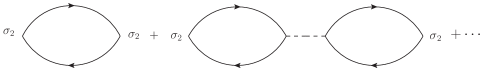
Figure 1: Diagrams for Nambu-Goldstone boson Green’s function. The solid line shows the electron propagator and the dashed line denotes the BCS pairing interaction.

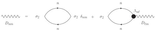
Figure 2: Diagrams for the equation of Nambu-Goldstone boson Green’s function. The solid line shows the electron propagator and the wavy line denotes the NG Green function. We introduced the vertex function indicated by the dot.

III.3 Poles of the NG boson Green’s function $D$

The energy dispersion of the NG mode is determined by the poles of the NG Green function. In general, we have one massless mode and $N-1$ gapped modes for an $N$-band superconductor. The poles depend on the intraband and interband couplings $g_{nm}$. We consider the case $\Sigma_{n}=0$ in this subsection. In this case we have $\tilde{\chi}=\chi$.

We assume that $v_{Fn}|{\bf q}|/q_{0}$ is small for $q=(q_{0},{\bf q})$. At absolute zero, we obtain

$$\chi_{NG,n}(q) = -N_{n}(0)\int d\xi_{k}\frac{1}{2E_{n}(\xi_{k})}$$ (37)

$$-N_{n}(0)\frac{\tilde{q}_{n}}{2\bar{\Delta}_{n}}\frac{1}{\sqrt{1-(\tilde{q}_{n}/2\bar{\Delta}_{n})^{2}}}$$

$$\times\tan^{-1}\left(\frac{\tilde{q}_{n}}{2\bar{\Delta}_{n}}\frac{1}{\sqrt{1-(\tilde{q}_{n}/2\bar{\Delta}_{n})^{2}}}\right),$$

for

$$\tilde{q}_{n}=\sqrt{q_{0}^{2}-\frac{1}{3}v_{Fn}^{2}{\bf q}^{2}},$$ (38)

where we used an approximation $({\bf v}_{F}\cdot{\bf q})^{2}\approx(1/3)v_{F}^{2}|{\bf q}|^{2}$. $q_{0}$ and ${\bf q}$ appear as a linear combination $q_{0}^{2}-(1/3)v_{Fn}^{2}{\bf q}^{2}$ for $v_{Fn}|{\bf q}|/q_{0}\ll 1$. The equation ${\rm det}(g^{-1}+\tilde{\chi})(q)=0$ determines the dispersion relation of the NG modes. We have one massless mode since ${\rm det}D^{-1}(q)$ vanishes as $q=(q_{0},{\bf q})\rightarrow 0$. $D(q)$ has a pole with a finite residue. Using $\tan^{-1}x=x-(1/3)x^{3}+\cdots$, for a single-band superconductor, the NG Green function for small $q_{0}$ and ${\bf q}$ is written as

$$D(q)\simeq 8N(0)\frac{1}{(gN(0))^{2}}\frac{(2\Delta)^{2}}{q_{0}^{2}-c_{s}^{2}{\bf q}^{2}},$$ (39)

where $c_{s}=v_{F}/\sqrt{3}$. In the two-band case, we obtain

$$D(q) = \tilde{D}(q)\Big{[}\frac{\gamma_{12}}{4\bar{\Delta}_{1}\bar{\Delta}_{2}}(N_{1}+N_{2})(q_{0}^{2}-v_{NG}^{2}{\bf q}^{2})$$ (40)

$$+\frac{N_{1}N_{2}}{16\bar{\Delta}_{1}^{2}\bar{\Delta}_{2}^{2}}(q_{0}^{4}-\frac{1}{3}(v_{F1}^{2}+v_{F2}^{2})q_{0}^{2}{\bf q}^{2})\Big{]}^{-1},$$

where

$$v_{NG}^{2}=\frac{1}{3}\frac{N_{1}v_{F1}^{2}+N_{2}v_{F2}^{2}}{N_{1}+N_{2}},$$ (41)

and we write $N_{m}=N_{m}(0)$. $\gamma_{nm}$ is the strength of Josephson coupling defined as the inverse of $g$:

$$\gamma_{nm}=(g^{-1})_{nm}.$$ (42)

There are corrections to the coefficient of $q_{0}^{4}$ and $q_{0}^{2}{\bf q}^{2}$, which are of the order of $\gamma_{12}$. We neglected them in eq.(36). $\tilde{D}(q)$ is a matrix given as

$$\tilde{D}(q) = g^{-1}\left(\begin{array}[]{cc}\gamma_{22}-f_{2}-N_{2}I(\frac{\tilde{q}_{2}}{2\bar{\Delta}_{2}})&-\gamma_{12}\\ -\gamma_{21}&\gamma_{11}-f_{1}-N_{1}I(\frac{\tilde{q}_{1}}{2\bar{\Delta}_{1}})\\ \end{array}\right)$$ (48)

$$\times\left(\begin{array}[]{cc}\chi_{1}(q)&0\\ 0&\chi_{2}(q)\\ \end{array}\right),$$

where we put

$$I(x)=\frac{x}{\sqrt{1-x^{2}}}\tan^{-1}\left(\frac{x}{\sqrt{1-x^{2}}}\right).$$ (50)

In deriving $D(q)$ in eq.(36), we used the gap equation written as

$$(\gamma_{11}-f_{1})\bar{\Delta}_{1}+\gamma_{12}\bar{\Delta}_{2} = 0,$$ (51)

$$\gamma_{21}\bar{\Delta}_{1}+(\gamma_{22}-f_{2})\bar{\Delta}_{2} = 0.$$ (52)

From zeros of the denominator of eq.(36), the dispersions of excitation modes (Nambu-Goldstone-Leggett modes) are determined. The Nambu-Goldstone mode has the dispersion $\omega_{NG}({\bf q})=v_{NG}|{\bf q}|$, and the massive mode hassha02

$$\omega_{NGL}({\bf q})^{2}=\omega_{L}^{2}+v_{L}^{2}{\bf q}^{2},$$ (53)

where

$$\omega_{L}=\sqrt{\frac{4|\gamma_{12}\bar{\Delta}_{1}\bar{\Delta}_{2}|\frac{N_{1}+N_{2}}{N_{1}N_{2}}}{1+\frac{2}{3}\gamma_{12}\left(\frac{1}{N_{1}}\frac{\bar{\Delta}_{1}}{\bar{\Delta}_{2}}+\frac{1}{N_{2}}\frac{\bar{\Delta}_{2}}{\bar{\Delta}_{2}}\right)}},$$ (54)

$$v_{L}^{2} = \frac{1}{3}\frac{N_{1}v_{F2}^{2}+N_{2}v_{F1}^{2}}{N_{1}+N_{2}}$$

$$+ \frac{2}{9}v_{F1}^{2}\left(\frac{\gamma_{12}}{N_{2}}\frac{\bar{\Delta}_{2}}{\bar{\Delta}_{1}}-\frac{\gamma_{12}}{N_{1}}\frac{\bar{\Delta}_{1}}{\bar{\Delta}_{2}}\right)$$

$$\times\left(1+\frac{2}{3}\gamma_{12}\left(\frac{1}{N_{1}}\frac{\bar{\Delta}_{1}}{\bar{\Delta}_{2}}+\frac{1}{N_{2}}\frac{\bar{\Delta}_{2}}{\bar{\Delta}_{2}}\right)\right)^{-1},$$

$$+ \frac{2}{9}v_{F2}^{2}\left(\frac{\gamma_{12}}{N_{1}}\frac{\bar{\Delta}_{1}}{\bar{\Delta}_{2}}-\frac{\gamma_{12}}{N_{2}}\frac{\bar{\Delta}_{2}}{\bar{\Delta}_{1}}\right)$$

$$\times\left(1+\frac{2}{3}\gamma_{12}\left(\frac{1}{N_{1}}\frac{\bar{\Delta}_{1}}{\bar{\Delta}_{2}}+\frac{1}{N_{2}}\frac{\bar{\Delta}_{2}}{\bar{\Delta}_{2}}\right)\right)^{-1}.$$

We included a correction of the order of $\gamma_{12}$. Here please note that when $\gamma_{12}<0$, we have $\bar{\Delta}_{1}\bar{\Delta}_{2}>0$, and when $\gamma_{12}>0$, $\bar{\Delta}_{1}\bar{\Delta}_{2}<0$ from the gap equation. Thus, $\gamma_{12}\bar{\Delta}_{1}\bar{\Delta}_{2}<0$.

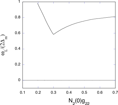
Figure 4: Gap energy of the Nambu-Goldstone-Leggett mode as a function of $N_{2}g_{22}$ for a two-band superconductor. We used $N_{1}g_{11}=0.3$ and $N_{1}g_{12}=0.02$. We set $\Delta_{m}=min(\bar{\Delta}_{1},\bar{\Delta}_{2})$ and $N_{1}(0)=N_{2}(0)$.

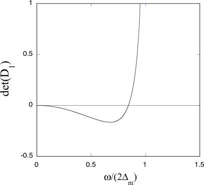
Figure 5: The determinant ${\rm det}D_{1}(\omega,{\bf q}=0)$ as a function of $\omega/(2\Delta_{m})$ where $D_{1}=g^{-1}+\chi$. The zero of ${\rm det}D_{1}$ indicates the excitation energy. We used $N_{1}g_{11}=0.3$, $N_{2}g_{22}=0.25$ and $N_{1}g_{12}=0.03$. We set $\Delta_{m}=min(\bar{\Delta}_{1},\bar{\Delta}_{2})$ and $N_{1}(0)=N_{2}(0)$.

We show the excitation energy as a function of $g_{12}$ for two-band superconductors in Fig. 3. There are two massless modes when $g_{12}=0$, and the one mode becomes massive for non-zero $g_{12}$. The excitation energy $\omega_{L}$ of the Leggett mode is dependent upon coupling constant $\{g_{nm}\}$. We show $\omega_{L}$ as a function of $g_{22}$ in Fig. 4 for a two-band superconductor. The excitation gap energy is determined as a zero of ${\rm det}D^{-1}(\omega,{\bf q}=0)$ which is shown in Fig. 5.

For a three-band superconductor, ${\rm det}(g^{-1}+\chi)$ is expanded as follows for small $q_{0}$ and ${\bf q}$:

$${\rm det}(g^{-1}+\chi)$$ (56)

$$= -\frac{N_{1}+N_{2}+N_{3}}{4(\bar{\Delta}_{1}\bar{\Delta}_{2}\bar{\Delta}_{3})^{2}}(\gamma_{12}\gamma_{13}\bar{\Delta}_{1}^{2}\bar{\Delta}_{2}\bar{\Delta}_{3}+\gamma_{12}\gamma_{23}\bar{\Delta}_{1}\bar{\Delta}_{2}^{2}\bar{\Delta}_{3}$$

$$+ \gamma_{13}\gamma_{23}\bar{\Delta}_{1}\bar{\Delta}_{2}\bar{\Delta}_{3}^{2})(q_{0}^{2}-v_{NG}^{2}{\bf q}^{2})$$

$$-\frac{1}{16(\bar{\Delta}_{1}\bar{\Delta}_{2}\bar{\Delta}_{3})^{2}}\big{[}N_{2}(N_{1}+N_{3})\gamma_{13}\bar{\Delta}_{1}\bar{\Delta}_{3}$$

$$+N_{1}(N_{2}+N_{3})\gamma_{23}\bar{\Delta}_{2}\bar{\Delta}_{3}+N_{3}(N_{1}+N_{2})\gamma_{12}\bar{\Delta}_{1}\bar{\Delta}_{2}\big{]}q_{0}^{4}$$

$$- \frac{1}{64(\bar{\Delta}_{1}\bar{\Delta}_{2}\bar{\Delta}_{3})^{2}}N_{1}N_{2}N_{3}q_{0}^{6}$$

$$+ \frac{1}{16(\bar{\Delta}_{1}\bar{\Delta}_{2}\bar{\Delta}_{3})^{2}}\big{[}N_{1}N_{2}(\gamma_{13}\bar{\Delta}_{1}\bar{\Delta}_{3}+\gamma_{23}\bar{\Delta}_{2}\bar{\Delta}_{3})$$

$$\times\frac{1}{3}(v_{F1}^{2}+v_{F2}^{2})+N_{2}N_{3}(\gamma_{12}\bar{\Delta}_{1}\bar{\Delta}_{2}+\gamma_{13}\bar{\Delta}_{1}\bar{\Delta}_{3})$$

$$\times\frac{1}{3}(v_{F2}^{2}+v_{F3}^{2})+N_{1}N_{3}(\gamma_{12}\bar{\Delta}_{1}\bar{\Delta}_{2}+\gamma_{23}\bar{\Delta}_{2}\bar{\Delta}_{3})$$

$$\times\frac{1}{3}(v_{F1}^{2}+v_{F3}^{2})\big{]}q_{0}^{2}{\bf q}^{2}+\cdots,$$

where we assume $\gamma_{nm}=\gamma_{mn}$ and used the gap equation for three gaps:

$$\left(\begin{array}[]{ccc}\gamma_{11}-f_{1}&\gamma_{12}&\gamma_{13}\\ \gamma_{21}&\gamma_{22}-f_{2}&\gamma_{23}\\ \gamma_{31}&\gamma_{32}&\gamma_{33}-f_{3}\\ \end{array}\right)\left(\begin{array}[]{c}\bar{\Delta}_{1}\\ \bar{\Delta}_{2}\\ \bar{\Delta}_{3}\\ \end{array}\right)=0.$$ (63)

The velocity for the NG mode in the three-band case is given by

$$v_{NG}^{2}=\frac{1}{3}\frac{N_{1}v_{F1}^{2}+N_{2}v_{F2}^{2}+N_{3}v_{F3}^{2}}{N_{1}+N_{2}+N_{3}}.$$ (64)

The velocity $v_{NG}$ in the $N$-band case is straightforwardly obtained as

$$v_{NG}^{2}=\frac{1}{3}\frac{N_{1}v_{F1}^{2}+\cdots+N_{N}v_{FN}^{2}}{N_{1}+\cdots+N_{N}}.$$ (65)

The gap $\omega_{L}$ of the massive mode is obtained as a zero of ${\rm det}(g^{-1}+\chi)$ in the limit ${\bf q}\rightarrow 0$, that is, a solution of the cubic equation for $q_{0}^{2}$. $\omega_{L}$ is given as

$$\omega_{L}^{2}=-\frac{2A_{1}}{A_{0}}\pm\frac{2}{A_{0}}\sqrt{A_{1}^{2}-4A_{0}A_{2}},$$ (66)

where

$$A_{0} = N_{1}N_{2}N_{3},$$ (67)

$$A_{1} = N_{1}(N_{2}+N_{3})\gamma_{23}\bar{\Delta}_{2}\bar{\Delta}_{3}+N_{2}(N_{1}+N_{3})\gamma_{13}\bar{\Delta}_{1}\bar{\Delta}_{3}$$ (68)

$$+N_{3}(N_{1}+N_{2})\gamma_{12}\bar{\Delta}_{1}\bar{\Delta}_{2},$$

$$A_{2} = (N_{1}+N_{2}+N_{3})\bar{\Delta}_{1}\bar{\Delta}_{2}\bar{\Delta}_{3}(\gamma_{12}\gamma_{13}\bar{\Delta}_{1}+\gamma_{12}\gamma_{23}\bar{\Delta}_{2}$$ (69)

$$+\gamma_{13}\gamma_{23}\bar{\Delta}_{3}).$$

Here we assumed that $A_{1}<0$ and $A_{1}^{2}-4A_{0}A_{2}\geq 0$. The lower energy gap is given by $(2/A_{0})(|A_{1}|-\sqrt{A_{1}^{2}-A_{0}A_{2}})$. If $A_{1}^{2}\gg A_{0}A_{2}$ is satisfied, this leads to $\omega_{L}^{2}\approx 4A_{2}/|A_{1}|$. When the contribution of one band is small, say $N_{3}\ll N_{1},N_{2}$, this gap reduces to that of the Leggett mode in the two-band case.

In the three-band case, there are in general three zeros in the determinant ${\rm det}D^{-1}(\omega,{\bf q}=0)$ as shown in Fig. 6. When $N\geq 3$, there is the case where several Leggett modes become massless. This is shown in Fig. 7 where the excitation energy $\omega_{L}$ is presented as a function of $g_{12}$. $\omega_{L}$ vanishes and one mode becomes massless when the time-reversal symmetry is broken.

Let us turn to examine $D(q)$ when $\tilde{q}_{n}\sim 2\bar{\Delta}_{n}$ ($\tilde{q}_{n}\leq 2\bar{\Delta}_{n}$). An analytic property of $\chi(q)$ will be changed as $q_{0}$ approaches the threshold energy $2\bar{\Delta}_{n}$. Using $\tan^{-1}(1/t)\simeq\frac{\pi}{2}-t+\frac{1}{3}t^{3}+\cdots$ for small $t>0$, we have

$$\chi_{n}(q)\simeq-f_{n}-N_{n}(0)\frac{\pi}{2}\frac{2\bar{\Delta}_{n}}{\sqrt{(2\bar{\Delta}_{n})^{2}+\frac{1}{3}v_{Fn}^{2}{\bf q}^{2}-q_{0}^{2}}},$$ (70)

for $\tilde{q}_{n}=\sqrt{q_{0}^{2}-\frac{1}{3}v_{Fn}^{2}{\bf q}^{2}}\simeq 2\bar{\Delta}_{n}$. In the single-band case, the Green function $D(q)$ is

$$D(q)\simeq\frac{8}{g}\left(1+\frac{1}{gN(0)\pi\bar{\Delta}}\sqrt{(2\bar{\Delta})^{2}+\frac{1}{3}v_{F}^{2}{\bf q}^{2}-q_{0}^{2}}+\cdots\right).$$ (71)

At the threshold $\tilde{q}=2\bar{\Delta}$, $D(q)$ becomes a constant: $D(q)\simeq 8/g$. $D(q)$ has no pole as a function of $q_{0}$ and loses a quasiparticle character in this region.

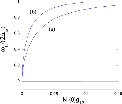
Figure 3: Gap energy of the Nambu-Goldstone-Leggett mode as a function of $N_{1}(0)g_{12}$ for two-band superconductors. The parameters are (a) $N_{1}(0)g_{11}=N_{2}(0)g_{22}=0.3$, and (b) $N_{1}(0)g_{11}=0.3$ and $N_{2}(0)g_{22}=0.25$. We set $\Delta_{m}=min(\bar{\Delta}_{1},\bar{\Delta}_{2})$ and $N_{1}(0)=N_{2}(0)$.

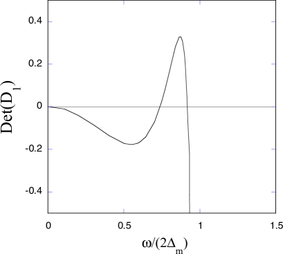
Figure 6: The determinant ${\rm det}D_{1}(\omega,{\bf q}=0)$ as a function of $\omega/(2\Delta_{m})$ for $D_{1}=g^{-1}+\chi$ in a three-gap case. The zero of ${\rm det}D_{1}$ indicates the excitation energy, There are three zeros in the three-gap case. We used $N_{1}g_{11}=N_{2}g_{22}=N_{3}g_{33}=0.3$, $N_{1}g_{12}=0.05$, $N_{1}g_{23}=0.04$ and $N_{1}g_{13}=0.02$. We set $\Delta_{m}=min(\bar{\Delta}_{1},\bar{\Delta}_{2},\bar{\Delta}_{3})$ and $N_{1}(0)=N_{2}(0)=N_{3}(0)$.

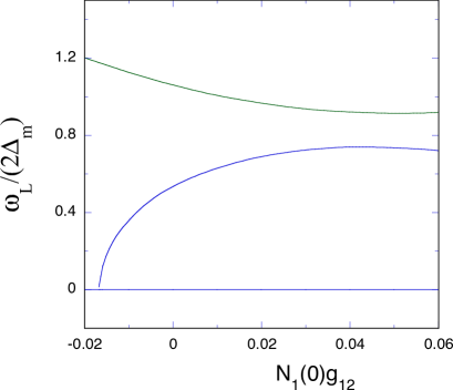
Figure 7: Gap energy of the Nambu-Goldstone-Leggett mode as a function of $N_{1}g_{12}$ in a three-gap case. The zero of ${\rm det}D_{1}$ indicates the excitation energy, There are three zeros in the three-gap case. We used $N_{1}g_{11}=N_{2}g_{22}=N_{3}g_{33}=0.3$, $N_{1}g_{23}=0.05$, and $N_{1}g_{23}=0.02$. We set $\Delta_{m}=min(\bar{\Delta}_{1},\bar{\Delta}_{2},\bar{\Delta}_{3})$ and $N_{1}(0)=N_{2}(0)=N_{3}(0)$.

III.4 Ward-Takahashi identity and impurity scattering

We investigate the effect of impurity scattering on the Nambu-Goldstone modes in superconductors. The Hamiltonian for impurity scattering that we consider is written as

$$H_{imp} = \sum_{i}\sum_{m\sigma}u_{1mm}({\bf r}-{\bf R}_{i})\psi_{m\sigma}^{{\dagger}}({\bf r})\psi_{m\sigma}({\bf r})$$ (72)

$$+ \sum_{i}\sum_{m}u_{2m}({\bf r}-{\bf R}_{i}){\bf S}_{i}\cdot{\bf s}_{mi}$$

$$\equiv \sum_{m}\sum_{\sigma\sigma^{\prime}}\psi_{m\sigma}^{{\dagger}}V_{m\sigma\sigma^{\prime}}\psi_{m\sigma^{\prime}}.$$

where ${\bf R}_{i}$ indicates the position of an impurity, ${\bf S}_{i}$ indicates the spin operator of the impurity spin and ${\bf s}_{mi}$ is the spin operator of the electron in the $m$-th band. Here we consider only the intra band scattering for simplicity because the interband scattering breaks the gauge invariance under $\psi_{m\sigma}\rightarrow e^{-i\theta_{m}}\psi_{m\sigma}$.

We introduce the matrix self-energy to take account of the electron scattering due to non-magnetic and magnetic impurities:

$$\Sigma_{m}=\left(\begin{array}[]{cc}\Sigma_{1m}&\Sigma_{2m}\\ \Sigma_{2m}^{*}&\Sigma_{1m}\\ \end{array}\right).$$ (75)

We write the Green function in the form,

$$G_{m}(k)=\left(\begin{array}[]{cc}G_{m\uparrow\uparrow}(k)&F_{m}(k)\\ F_{m}^{*}(k)&G_{m\downarrow\downarrow}(k)\\ \end{array}\right).$$ (78)

Here we use the finite-temperature formalism by putting $k_{0}\rightarrow i\omega_{n}$ where $\omega_{n}=(2n+1)\pi/\beta$ is the Matsubara frequencyagd . In the impurity scattering, self-energies are given askop01

$$\Sigma_{1m}(i\omega_{n},{\bf k}) = \frac{1}{2\pi\tau_{1m}}\int d\xi_{k}G_{m\uparrow\uparrow}(i\omega_{n},{\bf k}),$$ (79)

$$\Sigma_{2m}(i\omega_{n},{\bf k}) = \frac{1}{2\pi\tau_{2m}}\int d\xi_{k}F_{m}(i\omega_{n},{\bf k}),$$ (80)

where $\tau_{1m}$ and $\tau_{2m}$ indicate relaxation times in the $m$-th band due to impurity scattering. We have $\tau_{1m}=\tau_{2m}$ for scattering by non-magnetic impurities, and $\tau_{1m}\neq\tau_{2m}$ for magnetic impurities.

$\Sigma_{1m}$ and $\Sigma_{2m}$ are related as follows.

$$\Sigma_{1m}(i\omega_{n})=-\frac{i}{2\tau_{1m}}\frac{\omega_{n}+i\Sigma_{1m}}{\sqrt{(\omega_{n}^{2}+i\Sigma_{1m})^{2}+(\bar{\Delta}_{m}+\Sigma_{2m})^{2}}},\\$$ (81)

$$\Sigma_{2m}(i\omega_{n})=\frac{1}{2\tau_{2m}}\frac{\bar{\Delta}_{m}+\Sigma_{2m}}{\sqrt{(\omega_{n}^{2}+i\Sigma_{1m})^{2}+(\bar{\Delta}_{m}+\Sigma_{2m})^{2}}}.\\$$ (82)

We define $\tau_{sm}$ by

$$\frac{1}{\tau_{sm}}=\frac{1}{\tau_{1m}}-\frac{1}{\tau_{2m}}.$$ (83)

When $1/\tau_{sm}$ is small, $\Sigma_{1m}$ and $\Sigma_{2m}$ are expanded as

$$-\Sigma_{1m}(i\omega_{n}) = \frac{1}{2\tau_{1m}}\frac{i\omega_{n}}{\sqrt{\omega_{n}^{2}+\bar{\Delta}_{m}^{2}}}+\frac{1}{4\tau_{1m}\tau_{sm}}\frac{i\omega_{n}\bar{\Delta}_{m}^{2}}{(\omega_{n}^{2}+\bar{\Delta}_{m}^{2})^{2}},$$

$$\Sigma_{2m}(i\omega_{n}) = \frac{1}{2\tau_{2m}}\frac{\Delta_{n}}{\sqrt{\omega_{n}^{2}+\bar{\Delta}_{m}^{2}}}-\frac{1}{4\tau_{2m}\tau_{sm}}\frac{i\omega_{n}^{2}\bar{\Delta}_{m}}{(\omega_{n}^{2}+\bar{\Delta}_{m}^{2})^{2}},$$

The inverse Green function is expressed as

$$G_{n}^{-1}(i\omega,{\bf k})=\left(\begin{array}[]{cc}i\omega-\xi({\bf K})-\Sigma_{1m}&-\bar{\Delta}_{n}-\Sigma_{2n}\\ -\bar{\Delta}_{n}^{*}-\Sigma_{2n}^{*}&i\omega+\xi({\bf k})-\Sigma_{1n}\\ \end{array}\right).$$ (88)

The Ward-Takahashi identity is used to obtain a relation between the self-energy and the vertex function. The Ward-Takahashi identity is given askoy16 ; yan17

$$(q-k)_{\mu}G_{n}(k)\Gamma^{\mu}_{nm}(k,q)G_{n}(q)$$

$$~{}~{}~{}=i\delta_{nm}\sigma_{3}G_{n}(q)-i\delta_{nm}(k)\sigma_{3}-\lambda_{m}G_{n}(k)\Gamma_{nm}(k,q)G_{n}(q),$$

where

$$\Gamma_{nm}(k,q)=-2\delta_{nm}\sigma_{2}+\sum_{\ell}\Lambda_{n\ell}D_{\ell m}(q-k).$$ (91)

When $q\rightarrow k$, we have

$$iG_{n}^{-1}(k)\sigma_{3}-i\sigma_{3}G_{n}^{-1}(k)-\sum_{m}\lambda_{m}\Gamma_{nm}(k,k)=0.$$ (92)

The relation in eq.(11) is generalized to the multiband case as:

$$\sum_{m}\lambda_{m}D_{nm}(q\rightarrow 0)=-8\bar{\Delta}_{n},$$ (93)

as $\lambda_{m}\rightarrow 0$. Then we obtain

$$\sum_{m}\lambda_{m}\Gamma_{nm}(k,k)\rightarrow-8\sum_{\ell}\Lambda_{n\ell}(k,k)\bar{\Delta}_{\ell}$$ (94)

in the limit $\lambda_{m}\rightarrow 0$. This results in

$$iG_{n}^{-1}(k)\sigma_{3}-i\sigma_{3}G_{n}^{-1}(k)+8\sum_{\ell}\Lambda_{n\ell}(k,k)\bar{\Delta}_{\ell}=0.$$ (95)

The vertex function is determined as $\Lambda_{n\ell}=(1/4)\tilde{\Lambda}_{n}g_{n\ell}\sigma_{2}$ with

$$\tilde{\Lambda}_{n}=1+\frac{\Sigma_{2n}}{\bar{\Delta}_{n}}=1+\frac{1}{2\tau_{2n}}\frac{1}{\sqrt{\omega^{2}+\bar{\Delta}_{n}^{2}}}.$$ (96)

Here we used the gap equation given by

$$\bar{\Delta}_{n}=\sum_{\ell}g_{n\ell}\frac{1}{\beta}\sum_{\omega}\int\frac{d^{d}k}{(2\pi)^{d}}F_{\ell}(i\omega,{\bf k}).$$ (97)

From this relation, we can show that the NG boson Green function $D(q)$ has a pole at $q=(q_{0},{\bf q})=0$. In fact, the matrix $g^{-1}+\tilde{\chi}(q)$ in the limit $q\rightarrow 0$ is represented as

$$(g^{-1})_{n\ell}+\delta_{n\ell}\tilde{\chi}_{NG,n}(q=0)$$

$$= (g^{-1})_{n\ell}$$

$$-\delta_{n\ell}\frac{1}{\bar{\Delta}_{n}}N_{n}(0)\pi\frac{1}{\beta}\sum_{\omega}\frac{\bar{\Delta}_{n}+\Sigma_{2n}}{\sqrt{(\omega+i\Sigma_{1n})^{2}+(\bar{\Delta}_{n}+\Sigma_{2n})^{2}}}.$$

The determinant of this matrix vanishes because of the gap equation written as

$${\rm det}\left((g^{-1})_{n\ell}-\delta_{n\ell}\frac{1}{\bar{\Delta}_{n}}s_{n}\right)=0,$$ (99)

where

$$s_{n}=\pi N_{n}(0)\frac{1}{\beta}\sum_{\omega}\frac{\bar{\Delta}_{n}+\Sigma_{2n}}{\sqrt{(\omega+i\Sigma_{1n})^{2}+(\bar{\Delta}_{n}+\Sigma_{2n})^{2}}}.$$ (100)

IV Plasma mode

The Nambu-Goldstone mode becomes a massive plasma mode in the presence of the Coulomb potential. The plasma mode is represented by the spatial derivative of the phase variables $\theta_{n}$ where the order parameters are parametrized as $\Delta_{n}=e^{i2\theta_{n}}(\bar{\Delta}_{n}+h_{n})$. The action density for $\theta_{j}$ is written asyan15 ; yan17

$$\mathcal{L}[\theta] = \sum_{j}\Big{[}N_{j}(0)(\partial_{\tau}\theta_{j}-e\phi)^{2}+n_{j}\frac{1}{2m_{j}}(\nabla\theta_{j})^{2}\Big{]}$$

$$+ \frac{1}{8\pi}(\nabla\phi)^{2}+\sum_{ij}\bar{\Delta}_{i}(g^{-1})_{ij}\bar{\Delta}_{j}\cos(2(\theta_{i}-\theta_{j})),$$

where $e$ is the charge of the electron and $\phi$ indicates the Coulomb potential. The effective action for $\theta_{j}$ is obtained by integrating out the field $\phi$:

$$\mathcal{L}[\theta] = \frac{1}{8\pi e^{2}N(0)^{2}}\sum_{jj^{\prime}a}N_{j}(0)N_{j^{\prime}}(0)\partial_{\tau}\zeta_{ja}\partial_{\tau}\zeta_{j^{\prime}a}$$ (102)

$$+\sum_{ja}\frac{n_{j}}{2m_{j}}\zeta_{ja}^{2}+\sum_{j}N_{j}(0)\left(\partial_{\tau}\theta_{j}\right)^{2}$$

$$-\frac{1}{N(0)}\left(\sum_{j}N_{j}(0)\partial_{\tau}\theta_{j}\right)^{2}$$

$$+\sum_{ij}\bar{\Delta_{i}}(g^{-1})_{ij}\bar{\Delta_{j}}\cos(2(\theta_{i}-\theta_{j}))+\cdots,$$

where we put

$$\zeta_{ja}=\nabla_{a}\theta_{j},$$ (103)

and $N(0)=\sum_{j}N_{j}(0)$. The index $a$ takes $x$, $y$ and $z$.

In the single-band case, the plasma frequency is given by

$$\omega_{pl,a}^{2}=4\pi e^{2}n/m_{a},$$ (104)

where $n=n_{1}$ is the electron density. In the two-band case, the quadratic part of $\zeta_{ja}$ is written as

$$\frac{1}{\beta}\sum_{\ell}\frac{1}{8\pi e^{2}N(0)^{2}}\sum_{a}(\zeta_{1a}(\omega_{\ell})~{}\zeta_{2a}(\omega_{\ell}))M_{\zeta}\left(\begin{array}[]{c}\zeta_{1a}(-\omega_{\ell})\\ \zeta_{2a}(-\omega_{\ell})\\ \end{array}\right),$$ (107)

where

$$M_{\zeta}$$ (111)

$$= \left(\begin{array}[]{cc}\omega_{\ell}^{2}N_{1}(0)^{2}+\frac{4\pi e^{2}N(0)^{2}n_{1}}{m_{1a}}&\omega_{\ell}^{2}N_{1}(0)N_{2}(0)\\ \omega_{\ell}^{2}N_{1}(0)N_{2}(0)&\omega_{\ell}^{2}N_{2}(0)^{2}+\frac{4\pi e^{2}N(0)^{2}n_{2}}{m_{2a}}\\ \end{array}\right),$$

where $N(0)=N_{1}(0)+N_{2}(0)$. Then, the plasma frequency is given by the solution of ${\rm det}M_{\zeta}(i\omega_{\ell}\rightarrow\omega+i\delta)=0$:

$$\omega_{pl,a}^{2}=4\pi e^{2}\frac{n_{1}n_{2}}{m_{1a}m_{2a}}\frac{(N_{1}(0)+N_{2}(0))^{2}}{\frac{n_{1}}{m_{1a}}N_{2}(0)^{2}+\frac{n_{2}}{m_{2a}}N_{1}(0)^{2}}.$$ (113)

In an $N$-gap superconductor, the plasma frequency is generalized to be

$$\omega_{pl,a}^{2} = 4\pi e^{2}\frac{n_{1}\cdots n_{N}}{m_{1a}\cdots m_{Na}}N(0)^{2}\Big{[}N_{1}(0)^{2}\frac{n_{2}\cdots n_{N}}{m_{2a}\cdots m_{Na}}$$

$$+\cdots+N_{N}(0)^{2}\frac{n_{1}\cdots n_{N-1}}{m_{1a}\cdots m_{N-1,a}}\Big{]}^{-1},$$

for $a=x$, $y$ and $z$ where $N(0)=\sum_{j}N_{j}(0)$. When $N$ gaps are equivalent, this formula reduces to

$$\omega_{pl,a}^{2}=4\pi e^{2}\frac{n}{m_{a}}N.$$ (115)

V Higgs Green’s function in superconductors

V.1 Higgs Green’s function

The Green functions for the Higgs boson $h_{n}=\psi_{n}^{{\dagger}}\sigma_{1}\psi_{n}$ are defined by

$$H_{nm}(x-y)=-i\langle Th_{n}(x)h_{m}(y)\rangle.$$ (116)

The effective action for the Higgs fields, up to the one-loop order, is written as

$$S[h] = -\sum_{nm}\int dtd^{d}xh_{n}(g^{-1})_{nm}h_{m}$$ (117)

$$+\frac{i}{2}\sum_{n}{\rm Tr}h_{n}G_{n}^{(0)}(p)\sigma_{1}G_{n}^{(0)}(p+q)\sigma_{1}h_{n}.$$

When the temperature $T$ is near $T_{c}$, this gives the well-known time-dependent Ginzburg-Landau (TDGL) action. In the TDGL action, due to the dissipation effect, the Higgs mode may not be defined clearly. The Higgs mode is well defined at low temperatures.

The second term in the effective action eq.(117) for the Higgs field is the one-loop contribution given by

$$\Pi_{n}(i\epsilon,{\bf q}) = \frac{1}{2\beta}\sum_{n}\frac{1}{V}\sum_{{\bf p}}{\rm tr}\Big{[}G_{n}^{(0)}(i\omega_{n}+i\epsilon,{\bf p}+{\bf q})\sigma_{1}$$ (118)

$$\times G_{n}^{(0)}(i\omega_{n},{\bf p})\sigma_{1}\Big{]},$$

where we use the Matsubara formalism. At absolute zero, $\Pi_{n}(q_{0},{\bf q})$ (where $q_{0}=i\epsilon$) is expanded in $|{\bf q}|$ as

$$\Pi_{n}(q_{0},{\bf q}) = -N_{n}(0)\int d\xi\frac{1}{2E_{n}(\xi)}$$ (119)

$$+N_{n}(0)\left(4\bar{\Delta}_{n}^{2}-q_{0}^{2}\right)\frac{1}{4\bar{\Delta}_{n}^{2}}F\left(\frac{q_{0}}{2\bar{\Delta}_{n}}\right)$$

$$+N_{n}(0)\frac{1}{3}c_{ns}^{2}\left(\frac{{\bf q}}{2\bar{\Delta}_{n}}\right)^{2}+\cdots,$$

where $c_{ns}^{2}=v_{Fn}^{2}/3$ and $E_{n}(\xi)=\sqrt{\xi^{2}+\bar{\Delta}_{n}^{2}}$. $F(x)$ is given bykoy16

$$F(x) = \frac{1}{x\sqrt{1-x^{2}}}\tan^{-1}\left(\frac{x}{\sqrt{1-x^{2}}}\right)(0\leq x<1)$$ (120)

$$F(x) = -\frac{i}{x\sqrt{x^{2}-1}}\frac{\pi}{2}+\frac{1}{2x\sqrt{x^{2}-1}}\ln\Big{|}\frac{x-\sqrt{x^{2}-1}}{x+\sqrt{x^{2}-1}}\Big{|}$$ (121)

$$~{}~{}~{}~{}~{}(1<x).$$

We used an approximation that the density of states is constant.

When $q_{0}$ and ${\bf q}$ are small, we have for a single-band superconductor

$$\frac{1}{g}+\Pi(q_{0},{\bf q}) = N(0)\Big{[}1-\frac{1}{3}\left(\frac{q_{0}}{2\bar{\Delta}}\right)^{2}\Big{]}+N(0)\frac{1}{3}c_{s}^{2}\left(\frac{{\bf q}}{2\bar{\Delta}}\right)^{2}.$$

This is proportional to the inverse of the Fourier transform of the Higgs Green function. This agrees with the effective action for the Higgs mode obtained by means of the functional integral method given asyan17 ; ait99

$$S^{(2)}[h] = \int d\tau d^{d}xN(0)\Big{[}\frac{1}{12\bar{\Delta}^{2}}\left(\frac{\partial h}{\partial\tau}\right)^{2}+\frac{v_{F}^{2}}{36\bar{\Delta}^{2}}\left(\nabla h\right)^{2}$$ (123)

$$+h^{2}\Big{]},$$

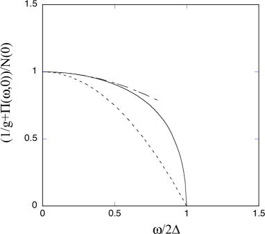
Figure 9: $g^{-1}+\Pi(\omega,{\bf q}=0)$ as a function of the $x\equiv\omega/2\bar{\Delta}$. The dash-dotted line shows the curve $1-x^{2}/3$. The dotted line indicates $1-x^{2}$ that corresponds to the Nambu-Jona-Lasinio model where $N(0)$ is replaced by the divergent integral $I_{0}\equiv(1/4\pi^{2})\ln(\Lambda/\bar{\Delta})$ with the cutoff $\Lambda$.

in the imaginary-time formulation. Please note that $1/g+\Pi(q)$ does not have a zero when $q_{0}$ is small as far as $0\leq q_{0}<2\bar{\Delta}$. We show the behavior of $F(x)$ in Fig.8 and $g^{-1}+\Pi(\omega,{\bf q}=0)$ as a function of $\omega$ in Fig.9.

When $v_{Fn}|{\bf q}|/q_{0}\ll 1$, the $g^{-1}+\Pi$ is given by

$$\left(g^{-1}+\Pi\right)_{mn} = (g^{-1})_{mn}-\delta_{mn}f_{n}$$

$$+ \delta_{mn}N_{n}(0)\Big{[}1-\left(\frac{\tilde{q}_{n}}{2\bar{\Delta}_{n}}\right)^{2}\Big{]}F\left(\frac{\tilde{q}_{n}}{2\bar{\Delta}_{n}}\right),$$

where we put

$$\tilde{q}_{n}=\sqrt{q_{0}^{2}-\frac{1}{3}v_{Fn}^{2}{\bf q}^{2}},$$ (125)

for the Fermi velocity $v_{Fn}$ in the $n$-th band.

We indicate the Fourier transform of the Higgs Green function $H_{nm}(x-y)$ as $H_{nm}(q)$:

$$H_{nm}(x)=\int\frac{dp_{0}}{2\pi}\frac{d^{d}p}{(2\pi)^{d}}e^{ip_{0}x_{0}+i{\bf p}\cdot{\bf x}}H_{nm}(p),$$ (126)

for $p=(p_{0},{\bf p})$. In a similar way as to the NG boson, the Higgs Green function satisfieskoy16

$$H_{nm}(q) = -i\int\frac{dk_{0}}{2\pi}\frac{d^{d}k}{(2\pi)^{d}}{\rm tr}\Big{[}\delta_{nm}\sigma_{1}G_{n}(k)\sigma_{1}G_{n}(k+q)$$

$$- \sum_{\ell}\sigma_{1}G_{n}(k)\Lambda_{H,n\ell}(k.k+q)G_{n}(k+q)H_{\ell m}(q)\Big{]},$$

where we introduced the vertex function $\Lambda_{H,n\ell}$. We can put this in the form

$$\Lambda_{H,n\ell}=\frac{1}{2}g_{n\ell}\sigma_{1}.$$ (128)

Then the matrix of Higgs Green’s function $H=(H_{nm})$ is written as follows.

$$H(q)=2g^{-1}(g^{-1}+\Pi(q))^{-1}\Pi(q),$$ (129)

where $\Pi(q)$ is the diagonal matrix with elements $\Pi_{n}(q)$ ($n=1,\cdots$): $\Pi(q)={\rm diag}(\Pi_{1}(q),\Pi_{2}(q),\cdots)$.

In the single-band case, the Higgs Green function for small $q_{0}$ and ${\bf q}$ is given by

$$H(q)\simeq 2N(0)\frac{1}{gN(0)}\frac{(2\bar{\Delta})^{2}}{(2\bar{\Delta})^{2}-\frac{1}{3}q_{0}^{2}+\frac{1}{3}c_{s}^{2}{\bf q}^{2}}.$$ (130)

When $q_{0}$ is as large as $2\bar{\Delta}$, $H(q)$ is approximated as

$$H(q)\approx-\frac{8}{\pi}N(0)\left(\frac{1}{gN(0)}\right)^{2}\frac{\bar{\Delta}}{\sqrt{\omega({\bf q})^{2}-q_{0}^{2}}}.$$ (131)

for $q_{0}<\omega({\bf q})$ where

$$\omega({\bf q})=\sqrt{(2\bar{\Delta})^{2}+\frac{1}{3}v_{F}^{2}{\bf q}^{2}}.$$ (132)

In the latter case, the singularity is given by a square root function. Thus, $H(q)$ represents a fluctuation mode, not a quasiparticle excitation mode since the residue at $q_{0}=\omega({\bf q})$ vanishes. $H(q)$ is defined on a Riemann surface with a cut from $q_{0}=-\omega({\bf q})$ to $q_{0}=\omega({\bf q})$ om the real axis. For $q_{0}>\omega({\bf q})$, there is the imaginary part representing the damping effect:

$$H(q)^{-1} \approx -\frac{1}{2}g^{2}N(0)\frac{1}{(2\bar{\Delta})^{2}}\left(q_{0}^{2}-\omega({\bf q})^{2}\right)$$ (133)

$$-i\frac{\pi}{4}g^{2}N(0)\frac{1}{2\bar{\Delta}}\sqrt{q_{0}^{2}-\omega({\bf q})^{2}},$$

when $q_{0}$ is near $\omega({\bf q})$. This behavior of the Higgs Green function is similar to that of the $\sigma$-particle Green function in the Gross-Neveu modelgro74 . The Higgs mode considered here has strong similarity with the $\sigma$ boson of the Gross-Neveu model in two dimensions. In fact, the Green function $G_{\sigma}(p)$, where $p=(p_{0},p_{1})$, of the $\sigma$ boson is given as up to the one-loop order

$$iG_{\sigma}(p)^{-1}=g^{2}\frac{N_{f}}{\pi}\sqrt{\frac{4\bar{\Delta}^{2}-p^{2}}{p^{2}}}\tan^{-1}\sqrt{\frac{p^{2}}{4\bar{\Delta}^{2}-p^{2}}},$$ (134)

for $0<p^{2}\equiv p_{0}^{2}-p_{1}^{2}<(2\bar{\Delta})^{2}$, and

$$iG_{\sigma}(p)^{-1} = -g^{2}\frac{N_{f}}{2\pi}\Bigg{[}\sqrt{\frac{p^{2}-4\bar{\Delta}^{2}}{p^{2}}}\ln\left|\frac{\sqrt{p^{2}}-\sqrt{p^{2}-4\bar{\Delta}^{2}}}{\sqrt{p^{2}}+\sqrt{p^{2}-4\bar{\Delta}^{2}}}\right|$$ (135)

$$~{}~{}+i\pi\sqrt{\frac{p^{2}-4\bar{\Delta}^{2}}{p^{2}}}\Bigg{]},$$

for $p^{2}>(2\bar{\Delta})^{2}$, where $N_{f}$ is the number of fermions and $g$ is the coupling constant in the Gross-Neveu model. For $p^{2}<0$ we have

$$iG_{\sigma}(p)^{-1}=-g^{2}\frac{N_{f}}{2\pi}\sqrt{\frac{-p^{2}+4\bar{\Delta}^{2}}{-p^{2}}}\ln\left|\frac{\sqrt{-p^{2}}-\sqrt{-p^{2}+4\bar{\Delta}^{2}}}{\sqrt{-p^{2}}+\sqrt{-p^{2}+4\bar{\Delta}^{2}}}\right|.$$ (136)

In the two-band case, the Higgs Green function is given as

$$H(q) = 2g^{-1}\left(\begin{array}[]{cc}\gamma_{11}+\Pi_{1}&\gamma_{12}\\ \gamma_{21}&\gamma_{11}+\Pi_{2}\\ \end{array}\right)^{-1}\left(\begin{array}[]{cc}\Pi_{1}&0\\ 0&\Pi_{2}\\ \end{array}\right)$$ (146)

$$= \frac{2}{(\gamma_{11}-f_{1})d_{2}+(\gamma_{22}-f_{2})d_{1}+d_{1}d_{2}}$$

$$\times\Big{[}\frac{1}{{\rm det}g}\left(\begin{array}[]{cc}\Pi_{1}&0\\ 0&\Pi_{2}\\ \end{array}\right)+\Pi_{1}\Pi_{2}\left(\begin{array}[]{cc}\gamma_{11}&\gamma_{12}\\ \gamma_{21}&\gamma_{22}\\ \end{array}\right)\Big{]},$$

where we set $\Pi_{n}(q)=-f_{n}+d_{n}(q)$ where

$$d_{n}(q)=N_{n}(0)\Big{[}1-\left(\frac{\tilde{q}_{n}}{2\bar{\Delta}_{n}}\right)^{2}\Big{]}F\left(\frac{\tilde{q}_{n}}{2\bar{\Delta}_{n}}\right),$$ (148)

and $\gamma_{nm}=(g^{-1})_{nm}$. We assume that $\gamma_{nm}=\gamma_{mn}$. Here we used the gap equation

$${\rm det}\left(\begin{array}[]{cc}\gamma_{11}-f_{1}&\gamma_{12}\\ \gamma_{21}&\gamma_{22}-f_{2}\\ \end{array}\right)=0.$$ (151)

It is seen from this expression that the Green function $H(q)$ shows no divergence when $\bar{\Delta}_{1}\neq\bar{\Delta}_{2}$ in general. This is shown in Fig. 10. The Higgs mode is not a quasiparticle mode and exists as a fluctuation mode in a multiband superconductor.

We define the Higgs constant potential $V=(V_{mn})$ as

$$V_{mn}=(g^{-1})_{mn}+\delta_{mn}\Pi_{n}(q_{0}=0,{\bf q}=0).$$ (152)

This is something like the ’mass term’ for Higgs fields $h_{n}$. In the subsection 5.4, we evaluate the eigenvalue $y_{H}^{2}$ of this matrix, by solving the gap equation. In a usual field theory, $y_{H}$ indicates the mass of the field $h$. In a superconductor, however, $y_{H}$ is different from the excitation gap because $y_{H}$ is not determined from a singularity of the Higgs Green function. The eigenvalues $y_{Hn}$, however, characterize the Higgs modes and determine the spatial expanse of the Higgs fields. In case ${\rm det}(V_{mn})=0$, one eigenvalue vanishes.

Figure 8: $F(x)$ as a function of $x=q_{0}/2\bar{\Delta}$. $F(x)$ has a singularity at $x=1$. The ’mass’ term is obtained by expanding $(1-x^{2})F(x)$ in terms of $x$.

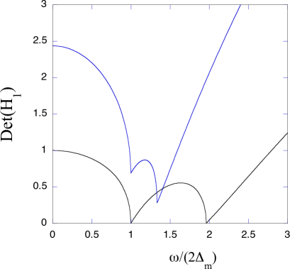
Figure 10: ${\rm det}H_{1}$ as a function of $\omega/2\Delta_{m}$ in a two-band case where $H_{1}={\rm Re}(g^{-1}+\Pi)$. The lower curve is for $N_{1}g_{11}=0.3$, $N_{2}g_{22}=0.25$ and $N_{1}g_{12}=0$ and the upper curve is for $N_{1}g_{11}=0.3$, $N_{2}g_{22}=0.25$ and $N_{1}g_{12}=0.05$. We put $\Delta_{m}=min(\bar{\Delta}_{1},\bar{\Delta}_{2},\bar{\Delta}_{3})$. When the interband $g_{12}$ vanishes, we have zeros at $\omega=\bar{\Delta}_{1}$ and $\omega=\bar{\Delta}_{2}$.

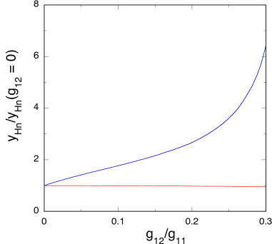
Figure 11: Eigenvalue $y_{H}^{2}$ in a two-band superconductor as a function of the interband coupling $g_{12}$. $y_{H}$ is measured in unit of that in the case of $g_{12}=0$. We set $g_{11}\bar{N}(0)=g_{22}\bar{N}(0)=0.35$ for $\bar{N}(0)=N_{1}(0)=N_{2}(0)$. The Higgs ’mass’ of one mode remains a constant whereas the other ’mass’ grows very large as $g_{12}$ increases.

V.2 Kinetic terms of the Higgs mode

We discuss the kinetic terms of Higgs boson in this subsection briefly, where the kinetic terms mean $(\partial_{\tau}h)^{2}$ and $(\nabla h)^{2}$. The time-dependent Ginzburg-Landau model with dissipation is often used in a study of nonequilibrium properties of superconductors near the critical temperature $T_{c}$. At low temperature $T\ll T_{c}$, the action for the Higgs mode is given by the quadratic from as shown in the previous subsection. Thus there is a temperature dependence. We consider here the single-band case for simplicity. The coefficient of $h\partial_{\tau}^{2}h$ is given as, up to the one-loop order,

$$I_{\tau}\equiv\frac{1}{\beta}\sum_{\ell}\frac{1}{V}\sum_{{\bf k}} \Big{[} \frac{\bar{\Delta}^{2}-\omega_{\ell}^{2}-\xi_{k}^{2}}{(\omega_{\ell}^{2}+\xi_{k}^{2}+\bar{\Delta}^{2})^{3}}-2\frac{\omega_{\ell}^{2}}{(\omega_{\ell}^{2}+\xi_{k}^{2}+\bar{\Delta}^{2})^{3}}$$ (153)

$$-4\frac{\bar{\Delta}^{2}-\omega_{\ell}^{2}-\xi_{k}^{2}}{(\omega_{\ell}^{2}+\xi_{k}^{2}+\bar{\Delta}^{2})^{4}}\omega_{\ell}^{2}\Big{]},$$

where $\xi_{k}$ denotes the electron dispersion relation. The coefficient of $h({\bf v}\cdot\nabla)^{2}h$ is similarly give by

$$I_{x}\equiv\frac{1}{\beta}\sum_{\ell}\frac{1}{V}\sum_{{\bf k}} \Big{[} \frac{\bar{\Delta}^{2}-\omega_{\ell}^{2}-\xi_{k}^{2}}{(\omega_{\ell}^{2}+\xi_{k}^{2}+\bar{\Delta}^{2})^{3}}-2\frac{\xi_{k}^{2}}{(\omega_{\ell}^{2}+\xi_{k}^{2}+\bar{\Delta}^{2})^{3}}$$ (154)

$$-4\frac{\bar{\Delta}^{2}-\omega_{\ell}^{2}-\xi_{k}^{2}}{(\omega_{\ell}^{2}+\xi_{k}^{2}+\bar{\Delta}^{2})^{4}}\xi_{k}^{2}\Big{]}.$$

At absolute zero, $I_{\tau}$ and $I_{x}$ are the same since we can exchange $\omega_{\ell}$ and $\xi_{k}$. When $T$ approaches $T_{c}$, $I_{\tau}$ vanishes at some $T$. Then, when $T\sim T_{c}$, the time-dependence of $h$ field should be given by the time-dependent Ginzburg-Landau functional. We show the kinetic terms at $T=0$ and $T\sim T_{c}$ in Table II.

Table 2: Kinetic terms of the Higgs field $h$ in the action at absolute zero $T\sim 0$ and near $T\sim T_{c}$ (for the single-band case).

	$T\sim 0$	$T\sim T_{c}$
$\tau$-part	$\frac{1}{12\bar{\Delta}^{2}}N(0)\left(\frac{\partial h}{\partial\tau}\right)^{2}$	$\frac{\pi\hbar}{8k_{B}T_{c}}hi\frac{\partial h}{\partial\tau}$
$x$-part	$\frac{1}{36\bar{\Delta}^{2}}N(0)\hbar^{2}v_{F}^{2}\left(\nabla h\right)^{2}$	$\frac{7\zeta(3)\hbar^{2}v_{F}^{2}}{48\pi^{2}k_{B}^{2}T_{c}^{2}}N(0)\left(\nabla h\right)^{2}$

V.3 Higgs constant potential

The Higgs constant potential $V$ is defined by $V=g^{-1}+\Pi$ in the limit of $q_{0}\rightarrow 0$ and ${\bf q}\rightarrow 0$. The potential $V$ in a multi-band superconductor is crucially dependent upon the coupling-constant matrix $g$. The quadratic from of $h_{n}$ in this limit is given as

$$M[h] \equiv \sum_{mn}h_{m}M_{mn}h_{n}$$ (155)

$$= \sum_{mn}h_{m}\left(\gamma_{mn}-\delta_{mn}f_{m}+\delta_{mn}\rho_{m}\right)h_{n},$$

where we set

$$\gamma_{mn} = (g^{-1})_{mn},$$ (156)

$$\rho_{m} = \int\frac{d^{d}k}{(2\pi)^{d}}\frac{1}{\beta}\sum_{\ell}\frac{2\bar{\Delta}_{m}^{2}}{(\omega_{\ell}^{2}+\xi_{k}^{2}+\bar{\Delta}_{m}^{2})^{2}}.$$ (157)

$\gamma_{mn}$ indicates the strength of the Josephson coupling between $m$ and $n$ bands. $\rho_{m}=\rho_{m}(T)$ equals the density of states $N_{m}(0)$ at absolute zero and is proportional to $\bar{\Delta}_{m}^{2}$ near $T_{c}$:

$$\rho_{m}=\left\{\begin{array}[]{cc}N_{m}(0)&{\rm at}~{}T=0,\\ N_{m}(0)\frac{7\zeta(3)}{4\pi^{2}k_{B}^{2}T_{c}^{2}}\bar{\Delta}_{m}(T)^{2}&{\rm for}~{}T\sim T_{c}.\\ \end{array}\right.$$ (160)

The gap function $\bar{\Delta}_{m}$ are determined by the gap equation,

$$\sum_{m}\gamma_{nm}\bar{\Delta}_{m}=f_{n}\bar{\Delta}_{n}.$$ (161)

In the single-band case, we have $M_{11}=\rho_{1}$ because of the gap equation. In the two-band case, $M=(M_{mn})$ is given by the $2\times 2$ matrix:

$$M=\left(\begin{array}[]{cc}\gamma_{11}-f_{1}+\rho_{1}&\gamma_{12}\\ \gamma_{21}&\gamma_{22}-f_{2}+\rho_{2}\\ \end{array}\right).$$ (164)

The critical temperature $T_{c}$ is given as

$$k_{B}T_{c}=\frac{2e^{\gamma}\omega_{c}}{\pi}e^{-\lambda},$$ (165)

where

$$\lambda = \frac{g_{11}/N_{2}+g_{22}/N_{1}}{2{\rm det}g}-\frac{1}{{\rm det}g}\sqrt{\frac{1}{4}\left(\frac{g_{11}}{N_{2}}-\frac{g_{22}}{N_{1}}\right)^{2}+\frac{g_{12}g_{21}}{N_{1}N_{2}}},$$

and $\omega_{c}$ is the cutoff. In the simple case where two bands are equivalent with $g_{11}=g_{22}$, $g_{12}=g_{21}$ and $N_{1}=N_{2}$, the superconducting gap at $T=0$ is

$$\bar{\Delta}_{1}=\bar{\Delta}_{2}=2\omega_{c}e^{-\lambda},$$ (167)

where

$$\lambda=\frac{1}{{\rm det}g}\left(\frac{g_{11}}{N_{1}}-\frac{|g_{12}|}{N_{1}}\right)=\frac{1}{(g_{11}+|g_{12}|)N_{1}}.$$ (168)

In this case, we must notice that $\Delta_{n}$ and $T_{c}$ are finite even when ${\det}g=0$.

When ${\rm det}g=0$, the gap functions are obtained as

$$\bar{\Delta}_{1} = 2\omega_{c}\exp\left(-\frac{1}{g_{11}N_{1}+g_{22}N_{2}}\left(1-\frac{1}{2}g_{22}N_{2}\ln\left(\frac{g_{22}}{g_{11}}\right)\right)\right),$$

for $g_{12}=g_{21}$. $\bar{\Delta}_{2}$ is obtained by exchanging the indices 1 and 2. This is in contrast to the single-band case where the vanishing of $g$ means the disappearance of superconductivity. A singular behavior of the ’mass’ spectra occurs when the determinant ${\rm det}g$ is small. We call the region with small ${\rm det}g$ the critical region in the following. We find that one of the eigenvalues of the matrix $M$ can be very large in this region.

V.4 Spectra of the Higgs potential in the two-band model

Let us consider the two-band case. There are two cases that should be examined; they are (a) ${\rm det}g>0$ and (b) ${\rm det}g<0$. Since the fields $h_{i}$ have the same dimension as $\Delta_{i}$, we define the fields $\eta_{n}$ by

$$h_{n}=\bar{\Delta}_{n}\eta_{n}.$$ (170)

Correspondingly, we define the Higgs mass matrix $\tilde{M}$ as

$$\tilde{M}=\left(\begin{array}[]{cc}(\gamma_{11}-f_{1}+\rho_{1})\bar{\Delta}_{1}^{2}&\gamma_{12}\bar{\Delta}_{1}\bar{\Delta}_{2}\\ \gamma_{12}\bar{\Delta}_{1}\bar{\Delta}_{2}&(\gamma_{22}-f_{2}+\rho_{2})\bar{\Delta}_{2}^{2}\\ \end{array}\right).$$ (173)

(a) Higgs modes for ${\rm det}g>0$.

In this case, ${\rm det}g=g_{11}g_{22}-g_{12}g_{21}>0$. The Josephson couplings $\gamma_{ij}$ are

$$\gamma_{11} = \frac{g_{22}}{{\rm det}g},~{}~{}\gamma_{22}=\frac{g_{11}}{{\rm det}g},~{}~{}\gamma_{12}=-\frac{g_{12}}{{\rm det}g}.$$

We assume that $g_{11}>0$ and $g_{22}>0$, namely, the interaction in each band is attractive. Then, w have $\gamma_{11}>0$ and $\gamma_{22}>0$. We also set $g_{12}=g_{21}$. When $\gamma_{12}=0$, the gap equation reduces to $\gamma_{nn}-f_{n}=0$ ($n=1,2$). For $\gamma_{12}\neq 0$, $f_{n}$ decreases, that is, $\bar{\Delta}_{n}$ increases, and thus $\gamma_{nn}-f_{n}>0$. The eigenvalues $x$ of $\tilde{M}$ are given as

$$x = \frac{1}{2}\{(\gamma_{11}-f_{1}+\rho_{1})\bar{\Delta}_{1}^{2}+(\gamma_{22}-f_{2}+\rho_{2})\bar{\Delta}_{2}^{2}\}$$ (176)

$$\pm\frac{1}{2}\Big{[}(\gamma_{11}-f_{1}+\rho_{1})\bar{\Delta}_{1}^{2}-(\gamma_{22}-f_{2}+\rho_{2})\bar{\Delta}_{2}^{2}$$

$$+4\gamma_{12}^{2}\bar{\Delta}_{1}^{2}\bar{\Delta}_{2}^{2}\Big{]}^{1/2}.$$

Let us consider, for simplicity, a simple model with equivalent two bands satisfying $g_{11}=g_{22}$, $N_{1}(0)=N_{2}(0)\equiv\bar{N}(0)$ and $\bar{\Delta}_{1}=\bar{\Delta}_{2}\equiv\bar{\Delta}$. This leads to $f_{1}=f_{2}$, $\rho_{1}=\rho_{2}$ and $\gamma_{11}-f_{1}=|\gamma_{12}|$. The eigenvalues of $\bar{M}$ are

$$x_{1}=\rho_{1}\bar{\Delta}^{2},~{}~{}x_{2}=(\rho_{1}+2|\gamma_{12}|)\bar{\Delta}^{2}.$$ (177)

The corresponding $y_{H1}$ and $y_{H2}$ are given by

$$y_{H1}=\sqrt{\frac{\rho_{1}}{\bar{N}(0)}}\bar{\Delta},~{}~{}y_{H2}=\sqrt{\frac{\rho_{1}+2|\gamma_{12}|}{\bar{N}(0)}}\bar{\Delta}.$$ (178)

The one mode $y_{H2}$ shows a dependence on $g_{12}$, while the other value remains a constant. $y_{H2}$ increases as $|g_{12}|$ increases as shown in Fig.11 for the two equivalent bands, with a very large value when ${\rm det}g$ is small. The Fig.12 indicates the superconducting gaps and $y_{H}$’s for $g_{11}N_{1}(0)=0.35$ and $g_{22}N_{2}(0)=0.30$ at absolute zero. The coherence length $\xi$ is proportional to the inverse of $y_{H}$, exhibiting the dependence on the coupling constant matrix $g$. Thus the upper critical field $H_{c2}$, being proportional to $1/\xi^{2}$, also shows the dependence on $g$. $H_{c2}$ can be very large as ${\rm det}g$ approaches zero.

(b) Higgs potential for ${\rm det}g<0$.

Let us turn to the case with ${\rm det}g=g_{11}g_{22}-g_{12}g_{21}<0$. We assume that $g_{11}>0$ and $g_{22}>0$. This means that $\gamma_{11}<0$ and $\gamma_{22}<0$. We examine the case with two equivalent bands. Since $\gamma_{11}<0$, we have $\gamma_{11}-f_{1}=-|\gamma_{12}|$. Then, the eigenvalues of the matrix $\bar{M}$ are

$$x_{1}=\rho_{1}\bar{\Delta}^{2},~{}~{}x_{2}=(\rho_{1}-2|\gamma_{12}|)\bar{\Delta}^{2}.$$ (179)

Correspondingly, we have

$$y_{H1}=\sqrt{\frac{\rho_{1}}{\bar{N}(0)}}\bar{\Delta},~{}~{}y_{H2}=\sqrt{\frac{\rho_{1}-2|\gamma_{12}|}{\bar{N}(0)}}\bar{\Delta}.$$ (180)

In constrast to the previous case, $y_{H2}$ decreases as $|\gamma_{12}|$ increases. Thus, the coherence length corresponding to $y_{H2}$ increases and can be very large as a function of $g_{12}|$. $y_{H2}$ decreases and vanishes when $|\gamma_{12}|$ increases as $|g_{12}|$ approaches $g_{11}$. The appearance of massless state indicates an instability of the superconducting state. When $y_{H2}^{2}<0$, the state with $(\bar{\Delta}_{1},\bar{\Delta}_{2})=(\bar{\Delta},\bar{\Delta})$ is at the saddle point and thus is instable to be away from this point. Let us examine this phenomenon in the following.

We include $\eta^{4}$ term in the action to investigate a stability of superconducting state. The mass functional is written as

$$M[\eta]=a_{1}\eta_{1}+a_{2}\eta_{2}+\eta^{t}\tilde{M}\eta+\frac{b}{4}(\eta_{1}^{4}+\eta_{2}^{4}),$$ (181)

with a constant $b>0$, where $\eta=^{t}(\eta_{1},\eta_{2})$. $\bar{\Delta}_{n}$ ($n=1,2$) are determined from the condition $a_{1}=a_{2}=0$. We write $\eta_{n}=\bar{\eta}_{n}+\delta\eta_{n}$ (for $n=1,2$) where $\bar{\eta}_{n}$ is a new stationary value of $\eta_{n}$ and $\delta\eta_{n}$ stands for fluctuation of the mode $\eta_{n}$. The condition that the linear terms in $\delta\eta_{n}$ should vanish results in the equations

$$2\tilde{M}_{11}\bar{\eta}_{1}+2\tilde{M}_{12}\bar{\eta}_{2}+b\bar{\eta}_{1}^{3} = 0,$$ (182)

$$2\tilde{M}_{12}\bar{\eta}_{1}+2\tilde{M}_{22}\bar{\eta}_{2}+b\bar{\eta}_{2}^{3} = 0.$$ (183)

Let us consider the model with two equivalent bands where we set $\bar{\Delta}\equiv\bar{\Delta}_{1}=\bar{\Delta}_{2}$ and $g_{11}=g_{22}$. The eigenvectors of the matrix $\bar{M}$ are ${}^{t}(1,1)/\sqrt{2}$ and ${}^{t}(1,-1)/\sqrt{2}$ with the eigenvalue $\rho_{1}\bar{\Delta}^{2}$ and $(\rho_{1}-2|\gamma_{12}|)\bar{\Delta}^{2}$, respectively. The eigenvalue corresponding to the mode $\eta_{1}-\eta_{2}$ can be negative and the state will show an instability to this direction. Then, we set $\bar{\eta}_{2}=-\bar{\eta}_{1}$ to obtain the equation

$$2(\rho_{1}-2|\gamma_{12}|)\bar{\Delta}^{2}+b\bar{\eta}_{1}^{2}=0,$$ (184)

for non-trivial solution $\bar{\eta}_{1}\neq 0$. Then we have

$$\bar{\eta}_{1}=\pm\sqrt{\frac{2(2|\gamma_{12}|-\rho_{1})}{b}}\bar{\Delta}.$$ (185)

Due to fluctuation of the $\eta_{1}-\eta_{2}$ mode, the stationary values of the gap functions $(\bar{\Delta}_{1},\bar{\Delta}_{2})$ change from $(\bar{\Delta},\bar{\Delta})$ to

$$(\bar{\Delta}+\bar{\eta}_{1}\bar{\Delta},\bar{\Delta}-\bar{\eta}_{1}\bar{\Delta}).$$ (186)

This is shown schematically in Fig. 13. Thus, the stationary values of $\Delta_{n}$ break the symmetry $\Delta_{1}=\Delta_{2}$ which should hole for the case of two equivalent bands, when ${\rm det}g<0$ and $\rho_{1}-2|\gamma_{12}|<0$. This may be called the spontaneous symmetry breaking of ${\bf Z}_{2}$ symmetry.

Near $((1+\bar{\eta}_{1})\bar{\Delta},(1-\bar{\eta}_{1})\bar{\Delta})$, the potential $M[\eta]$ is expanded as

$$M[\eta]={\rm const.}+^{t}\delta\eta\left(\begin{array}[]{cc}\tilde{M}_{11}+\frac{3}{2}b\bar{\eta}_{1}^{2}&\tilde{M}_{12}\\ \tilde{M}_{21}&\tilde{M}_{22}+\frac{3}{2}b\bar{\eta}_{2}^{2}\\ \end{array}\right)\delta\eta,$$ (189)

where $\delta\eta=^{t}(\delta\eta_{1},\delta\eta_{2})$. The eigenvalues of this $2\times 2$ matrix give $y_{H}$’s for Higgs modes. For the case with two equivalent bands, we have

$$y_{H1}^{2}=\frac{2(3|\gamma_{12}|-\rho_{1})}{\bar{N}(0)}\bar{\Delta}^{2},~{}~{}y_{H2}^{2}=\frac{2(2|\gamma_{12}|-\rho_{1})}{\bar{N}(0)}\bar{\Delta}^{2}.$$ (191)

This is shown in Fig.14 where $y_{Hn}^{2}$ for $n=1,2$ are shown as a function of $|\gamma_{12}|/\rho_{1}$. One mode becomes massless when $2|\gamma_{12}|=\rho_{1}$. When $2|\gamma_{12}|>\rho_{1}$, namely, $g_{12}^{2}$ is near $g_{11}g_{22}$, the Higgs values $y_{H}$ can be very large.

As we have shown above, the eigenvalues of Higgs matrix $M$ exhibit a singular behavior when ${\rm det}g$ is small. When ${\rm det}g>0$, the eigenvalue and thus $H_{c2}$ can be large. When ${\rm det}g<0$, there is a possibility of softening of the eigenvalue of one Higgs mode. We show $y_{Hn}^{2}$ as a function of $g_{12}$ in Fig.15. There is a singularity in the critical region near ${\rm det}g=0$, which shows a possibility of large upper critical field $H_{c2}$.

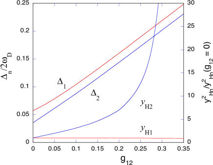
Figure 12: Gap functions $\bar{\Delta}_{n}$ and Higgs eigenvalue $y_{Hn}$ in a two-band superconductor ($n=1,2$) as a function of the interband coupling $g_{12}$. $y_{Hn}$ is measured in unit of that in the case of $g_{12}=0$. We set $g_{11}\bar{N}(0)=0.35$ and $g_{22}\bar{N}(0)=0.30$ for $\bar{N}(0)=N_{1}(0)=N_{2}(0)$. The Higgs eigenvalue of one mode remains a constant whereas the other grows very large as $g_{12}$ increases, namely ${\rm det}g$ approaches zero. $\Delta_{n}$ in the figure indicates $\bar{\Delta}_{n}$.

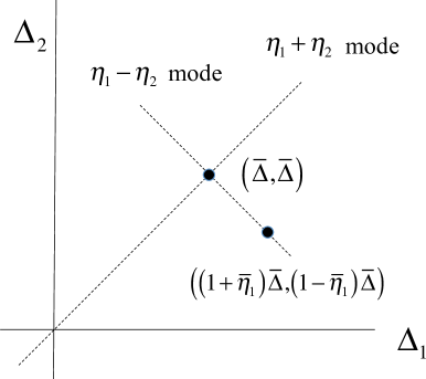
Figure 13: Gap functions and fluctuation modes when two bands are equivalent for ${\rm det}g<0$ and $\rho_{1}-2|\gamma_{12}|<0$. The order parameters $(\bar{\Delta},\bar{\Delta})$ is shifted to $((1+\bar{\eta}_{1})\bar{\Delta},(1-\bar{\eta}_{1})\bar{\Delta})$ or $((1-\bar{\eta}_{1})\bar{\Delta},(1+\bar{\eta}_{1})\bar{\Delta})$ due to the fluctuation of $\eta_{1}-\eta_{2}$ mode.

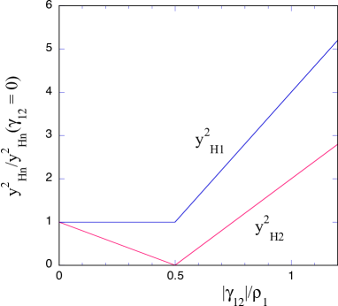
Figure 14: $y_{Hn}^{2}$ ($n=1,2$) as a function of $|\gamma_{12}|$ when ${\det}g<0$. In this case, the region with small $\gamma_{12}$ is unrealistic because $g_{12}$ should be very small. We used $g_{11}N_{1}(0)=0.30$.

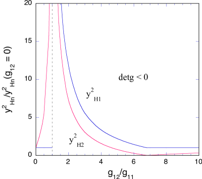
Figure 15: $y_{Hn}^{2}$ ($n=1,2$) as a function of $g_{12}/g_{11}$ where $g_{12}>0$. We have ${\det}g<0$ for $g_{12}/g_{11}>1$. $y_{Hn}$ shows a singularity near ${\det}g=0$.

V.5 Higgs potential in a three-band superconductor

We turn to a three-band superconductor in this subsection. The Higgs matrix $M$ is given by

$$M=\left(\begin{array}[]{ccc}\gamma_{11}-f_{1}+\rho_{1}&\gamma_{12}&\gamma_{13}\\ \gamma_{21}&\gamma_{22}-f_{2}+\rho_{2}&\gamma_{33}\\ \gamma_{31}&\gamma_{32}&\gamma_{33}-f_{3}+\rho_{3}\\ \end{array}\right).$$ (195)

Let us first consider the case where three bands are equivalent, that is, we have $g_{11}=g_{22}=g_{33}\equiv t>0$ and $g_{12}=g_{21}=g_{23}=g_{32}=g_{31}=g_{13}\equiv v$. We have also the same density of state in every band as $N_{1}(0)=N_{2}(0)=N_{3}(0)\equiv\bar{N}(0)$ and $\rho_{1}=\rho_{2}=\rho_{3}\equiv\rho$, and thus $f_{1}=f_{2}=f_{3}\equiv f$. In this case the matrix $g$ of coupling constants is

$$g=\left(\begin{array}[]{ccc}t&v&v\\ v&t&v\\ v&v&t\\ \end{array}\right).$$ (200)

Then, ${\rm det}g=(t-v)^{2}(t+2v)$ and the Josephson couplings $\gamma_{ij}$ are

$$\gamma_{ii}=\frac{t+v}{(t-v)(t+2v)},~{}~{}\gamma_{ij}=-\frac{v}{(t-v)(t+2v)}~{}(i\neq j).$$ (201)

The gap equation is written as

$$\left|\begin{array}[]{ccc}\gamma_{11}-f_{1}&\gamma_{12}&\gamma_{13}\\ \gamma_{21}&\gamma_{22}-f_{1}&\gamma_{23}\\ \gamma_{31}&\gamma_{32}&\gamma_{33}-f_{3}\\ \end{array}\right|=0.$$ (205)

In our simple case, the critical temperature is given by

$$k_{B}T_{c}=\frac{2e^{\gamma_{E}}}{\pi}\omega_{D}\exp\left(-\frac{1}{(g_{11}+2g_{12})\bar{N}(0)}\right),$$ (206)

when $v=g_{12}>0$, and

$$k_{B}T_{c}=\frac{2e^{\gamma_{E}}}{\pi}\omega_{D}\exp\left(-\frac{1}{(g_{11}+|g_{12}|)\bar{N}(0)}\right),$$ (207)

when $v=g_{12}<0$. The eigenvalues of the matrix $M$ are

$${\rm(A)}~{}~{}~{}x_{1} = \rho,~{}~{}x_{2}=\rho-2\gamma_{12}~{}~{}{\rm for}~{}v>0,$$ (208)

$${\rm(B)}~{}~{}~{}x_{1} = \rho,~{}~{}x_{2}=\rho+3\gamma_{12}~{}~{}{\rm for}~{}v<0.$$ (209)

For $v>0$, the eigenstates with $\rho-2\gamma_{12}$ are doubly degenerate. On the other hand, for $v<0$, the states with the eigenvalue $\rho$ are doubly degenerate. We call these two cases the case A and B, respectively. In the case A, since $\gamma_{12}$ is negative for $0<v<g_{11}$, two eigenvalues of the Higgs matrix $M$ increase as $|\gamma_{12}|$ increases. $\rho-3\gamma_{12}$ diverges at the critical point ${\rm det}g=0$. In contrast, in the case B, one Higgs mode has a large $y_{H}$ in the critical region where ${\rm det}g$ is small.

We present a typical behavior of $y_{Hn}$ as a function of $g_{12}$ for the case with three equivalent bands in Fig.16. The ’mass’ of one mode remains constant as in the case of two-band superconductivity. We show $y_{Hn}$ for two cases as a function of $g_{12}$ in Figs.17 and 18 where three bands are not necessarily equivalent. In Fig.17 $y_{Hn}$ of two modes show a large dependence of $g_{12}$ indicating that this is in the case A.

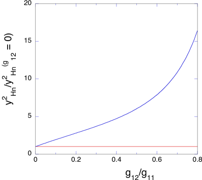
Figure 16: $y_{Hn}^{2}$ ($n=1,2,3$) as a function of $g_{12}/g_{11}$ for the model with three equivalent bands where we assume $g_{11}=g_{22}=g_{33}$, $g_{12}=g_{23}=g_{31}$ and $N_{1}(0)=N_{2}(0)=N_{3}(0)$. We set $g_{11}N_{1}(0)=0.3$. Two Higgs values grows large as $g_{12}(>0)$ increases in the case A. In the case B, the label of the horizontal axis should read $2|g_{12}|/g_{11}$ for $g_{12}<0$ and we have a similar behavior. One of Higgs modes has a heavy $y_{H}$ for large $|g_{12}|/g_{11}$ in the case A. The heavy eigenvalue becomes very huge in the critical region where ${\rm det}g\sim 0$.

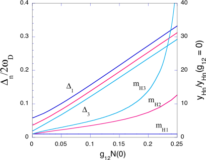
Figure 17: $\bar{\Delta}_{n}$ and $y_{Hn}^{2}$ ($n=1,2,3$) as a function of $g_{12}/g_{11}$ where we assume $g_{12}=g_{23}=g_{31}$. We set $g_{11}N_{1}(0)=0.35$, $g_{22}N_{2}(0)=0.3$ and $g_{33}N_{3}(0)=0.25$. We adopt that we have the same density of states in three bands. Two of Higgs modes have a heavy value.

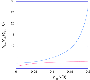
Figure 18: $y_{Hn}^{2}$ ($n=1,2,3$) as a function of $g_{12}\bar{N}(0)$ where we assume $g_{12}=g_{31}$. We used a set parameters as $g_{11}\bar{N}(0)=0.35$, $g_{22}\bar{N}(0)=0.30$, $g_{33}\bar{N}(0)=0.25$ and $g_{23}\bar{N}(0)=0.05$. We also adopt that $N_{1}(0)=N_{2}(0)=N_{3}(0)=\bar{N}(0)$. In this case, the value of $y_{H}$ of one Higgs mode becomes large as $g_{12}$ increases.

Let us investigate the case where $y_{Hn}^{2}$ is negative when $|g_{12}|$ becomes large across the critical point ${\rm det}g=0$. In the case B with isotropic three bands, the one mode has negative $y_{H1}^{2}$ for $v=g_{12}<-t/2=-g_{11}/2$. The mode $\eta\equiv(\eta_{1}+\eta_{2}+\eta_{3})/\sqrt{3}$ shows an instability in this case. We must include the $(b/4)\sum_{i}\eta_{i}^{4}$ ($b>0$) in the mass functional $M[\eta_{i}]$ to examine a stability of superconducting state. We express the shift of the stationary point of the gap functions as $\eta_{n}=\bar{\eta}+\delta\eta_{n}$. We obtain

$$\bar{\eta}=\pm\sqrt{\frac{2|\rho+3\gamma_{12}|}{b}},$$ (210)

for $\rho+3\gamma_{12}<0$. Then, the Higgs matrix $M$ is

$$M=\left(\begin{array}[]{ccc}8|\gamma|-2\rho&\gamma&\gamma\\ \gamma&8|\gamma|-2\rho&\gamma\\ \gamma&\gamma&8|\gamma|-2\rho\\ \end{array}\right),$$ (214)

where $\gamma=\gamma_{12}$. The eigenvalues are

$$x_{1}=9|\gamma|-2\rho,~{}~{}x_{2}=6|\gamma|-2\rho,$$ (215)

where the eigenstates with the eigenvalue $x_{1}=9|\gamma|-2\rho$ are doubly degenerate. The Higgs value squared $y_{Hn}^{2}\propto x_{n}$ is shown as a function of $\gamma=\gamma_{12}$ for the case of three equivalent bands with $g_{12}<0$ in Fig.19. $x_{2}$ vanishes at $|\gamma|=\rho/3$ and is large for large $|\gamma|$.

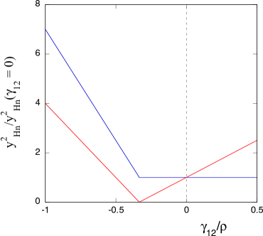
Figure 19: $y_{Hn}^{2}$ ($n=1,2,3$) as a function of $\gamma_{12}/\rho_{1}$ where we assume an isotropic three-band superconductor and $g_{12}<0$ (the case B in the text). We adopted that $g_{11}=g_{22}=g_{33}$, $g_{ij}$ ($i\neq j$) are the same, and $N_{1}(0)=N_{2}(0)=N_{3}(0)$. In this model, two Higgs states are degenerate and the other one state becomes a massless mode at $\gamma_{12}/\rho_{1}=-1/3$.

V.6 Discussion

We have considered the Higgs modes in multi-gap superconductors. Since the upper critical field $H_{c2}$ is proportional to $y_{H}^{2}$, there is a possibility that we have large $H_{c2}$ in a multi-gap superconductor such as iron-based superconductors by tuning interaction parameters. The eigenvalue $y_{H}$ increases as $|{\rm det}g|$ decreases. In a two-gap superconductor, we have two solutions for the gap equation and one solution with higher $T_{c}$ is realized. The other solution with low $T_{c}$ is expected to be less important. When the coherence length of low-$T_{c}$ solution is shorter than that of the high-$T_{c}$ solution, we expect that the low-$T_{c}$ solution plays a role in determining the critical field. As a result the upper critical field may be larger. This gives a possibility of high upper critical field in a multi-gap superconductor.

VI Summary

We have examined the property of Green’s functions of the Nambu-Goldstone and Higgs modes in a superconductor. In an $N$-gap superconductor, there are $N$ Nambu-Goldstone modes. We have, however, one gapless mode and $N-1$ massive modes in the presence of interband BCS couplings. The NG mode Green function $D(\omega,{\bf q})$ for small $\omega$ and ${\bf q}$ is given as $D\propto 1/(\omega^{2}-\omega({\bf q})^{2})$ with the dispersion $\omega({\bf q})=v_{NG}|{\bf q}|$ where $v_{NG}=(1/\sqrt{3})\sqrt{(N_{1}v_{F1}^{2}+\cdots+N_{N}v_{FN}^{2})/(N_{1}+\cdots+N_{N})}$. An analytic property of the NG Green function $D(\omega,{\bf q})$ is dependent on $\omega$. One gapless mode remains gapless in the presence of intraband scattering due to non-magnetic and magnetic impurities, which was shown on the basis of the Ward-Takahashi identity. In a multiband superconductor, massive modes due to interband couplings $g_{nm}$ become gapless again in a region with time-reversal symmetry breaking.

The Higgs Green function was also examined. The time-dependent part of the Higgs action is dependent on the temperature; it is given by $(\partial_{t}h)^{2}$ at low temperature, while it is $h\partial_{t}h$ near the critical temperature $T_{c}$. The Green function $H(\omega,{\bf q})$ of the Higgs mode has a singularity at $\omega\sim 2\Delta$ given as $2\Delta/\sqrt{(2\Delta)^{2}+\frac{1}{3}v_{F}^{2}{\bf q}^{2}-\omega^{2}}$. The Higgs Green function has the same singularity as the $\sigma$-boson Green function in the Gross-Neveu model. We have shown that when there are several order parameters, the constant part of the Higgs action is important and crucially dependent upon the interband coupling constants $g_{ij}$. In a multiband superconductor, the eigenvalue of the matrix $M$ of constant Higgs potential can be very large as the interband coupling constant $g_{12}$ increases, although the other eigenvalues of the other Higgs mode remain constant. This indicates the possibility of the large upper critical field $H_{c2}$ because of the relation $H_{c2}\propto 1/\xi^{2}\propto y_{H}^{2}$. In iron-based superconductors, the extremely huge $H_{c2}$ has been reported for NdFeAsO_0.7F_0.3jar08 and Ba_0.6K_0.4Fe₂As₂wan08 . Our results indicate that the huge $H_{c2}$ may be due to the multiband effect for the Higgs modes.

This work was supported in part by Grant-in-Aid from the Ministry of Education, Culture, Sports, Science and Technology of Japan (Grants No. 22540381 and No. 17K05559).

References

- (1) J. Goldstone, Nuovo Cimento 9, 154 (1961).
- (2) Y. Nambu, Phys. Lett. 4, 380 (1960).
- (3) J. Goldstone, A. Salam and S. Weinberg, Phys. Rev. 127, 965 (1962).
- (4) S. Weinberg, The Quantum Theory of Fields Vol. II (Cambridge University Press, Cambridge, 1995).
- (5) V. L. Ginzburg and L. D. Landau, Zh. Eksp. Teor. Fiz. 20, 1064 (1950).
- (6) J. Bardeen, L. N. Cooper and J. R. Schrieffer, Phys. Rev. 108, 1175 (1957).
- (7) P. W. Anderson, Basic Notions of Condensed Matter Physics (Benjamin/Cummings Publishing Company, London, 1984).
- (8) A. A. Abrikosov, Foundations of the Theory of Metals (North-Holland, Amsterdam, 1988).
- (9) R. M. White, Qunatum Theory of Magnetism (Springer, Berlin, 2006).
- (10) N. Goldenfeld, Lectures on Phase Transitions and the Renormalization Group (Perseus Books, Nassachusetts, 1992).
- (11) Y. Nambu and G. Jona-Lasinio, Phys. Rev. 122, 345 (1961).
- (12) P. W. Higgs, Phys. Rev. Lett. 13, 508 (1964).
- (13) M. L. Goldberger and T. Treiman, Phys. Rev. 111, 354 (1966).
- (14) S. Weinberg, Phys. Rev. Lett. 29, 1698 (1972).
- (15) H. B. Nielsen and S. Chadha, Nucl. Phys. B105, 445 (1976).
- (16) S. Coleman, Aspects of Symmetry (Cambridge University Press, Cambridge, 1985).
- (17) T. Brauner, Symmetry 2, 609 (2010).
- (18) H. Watanabe and H. Murayama, Phys. Rev. Lett. 108, 251602 (2012),
- (19) Y. Hidaka, Phys. Rev. Lett. 110, 091601 (2013).
- (20) K. Odagiri and T. Yanagisawa, Eur. Phys. J. C73, 2525 (2013).
- (21) T. Yanagisawa, Europhys. Lett. 113, 41001 (2016).
- (22) J. Bardeen, L. N. Cooper and J. R. Schrieffer, Phys. Rev. 108, 1175 (1957).
- (23) V. A. Moskalenko, Fiz. Metal and Metallored 8, 2518 (1959).
- (24) H. Suhl, B. T. Mattis and L. W. Walker: Phys. Rev. Lett. 3, 552 (1959).
- (25) J. Peretti, Phys. Lett. 2, 275 (1962).
- (26) J. Kondo: Prog. Theor. Phys. 29, 1 (1963).
- (27) V. Stanev and Z. Tesanovic, Phys. Rev. B81, 134522 (2010).
- (28) Y. Tanaka and T. Yanagisawa, J. Phys. Soc. Jpn. 79, 114706 (2010).
- (29) Y. Tanaka and T. Yanagisawa, Solid State Commun. 150, 1980 (2010).
- (30) R. G. Dias and A. M. Marques, Supercond. Sci. Technol. 24, 085009 (2011).
- (31) T. Yanagisawa, Y. Tanaka, I. Hase and K. Yamaji: J. Phys. Soc. Jpn. 81, 024712 (2012).
- (32) X. Hu and Z. Wang, Phys. Rev. B85, 064516 (2012).
- (33) V. Stanev, Phys. Rev. B85, 174520 (2012).
- (34) C. Platt, R. Thomale, C. Homerkamp, S. C. Zhang and W. Hanke, Phys. Rev. B85, 180502 (2012).
- (35) S. Maiti and A. V. Chubukov, Phys. Rev. B87, 144511 (2013).
- (36) B. J. Wilson and M. P. Das, J. Phys. Condens. Matter 25, 425702 (2013).
- (37) R. Ganesh, G. Baskaran, J. van den Brink and D. V. Efremov, Phys. Rev. Lett. 113, 177001 (2014).
- (38) Y. S. Yerin, A. N. Omelyanchouk and E. Il’ichev, Super. Sci. tech. 28, 095006 (2015).
- (39) A. D. Hillier, J. Quintanilla and R. Cywinskii, Phys. Rev. Lett. 102, 117007 (2009).
- (40) I. Hase and T. Yanagisawa, J. Phys. Soc. Jpn. 78, 084724 (2009).
- (41) T. Yanagisawa and I. Hase, J. Phys. Soc. Jpn. 82, 124704 (2013).
- (42) S. Z. Lin and X. Hu, New J. Phys. 14, 063021 (2012).
- (43) K. Kobayashi, M. Machida, Y. Ota and F. Nori, Phys. Rev. B88, 224516 (2013).
- (44) T. Koyama, J. Phys. Soc. Jpn. 83, 074715 (2014).
- (45) T. Yanagisawa and Y. Tanaka, New J. Phys. 16, 123014 (2014).
- (46) Y. Tanaka et al., Physica C516, 10 (2015).
- (47) H. Y. Choi et al., Phys. Rev. B80, 052505 (2009).
- (48) P. M. Shirage et al., Phys. Rev. Lett. 103, 257003 (2009).
- (49) T. Yanagisawa et al., J. Phys. Soc. Jpn. 78, 094718 (2009).
- (50) Yu. A. Izyumov and V. M. Laptev, Phase Transitions 20, 95 (1990).
- (51) G. E. Volovik, The Universe in a Helium Droplet (Oxford University Press, Oxford, 2009).
- (52) Y. Tanaka, Phys. Rev. Lett. 88, 017002 (2002).
- (53) S. V. Kuplevakhsky, A. N. Omelyanchouk and Y. S. Yerin: J. Low Temp. Phys. 37, 667 (2011).
- (54) Y. Tanaka, H. Yamamori, T. Yanagisawa, T. Nishio and S. Arisawa, Physica C548, 44 (2018).
- (55) T. Yanagisawa, I. Hase and Y. Tanaka, Phys. Lett. A382, 3483 (2018).
- (56) P. B. Littlewood and C. M. Varma, Phys. Rev. B26, 4883 (1982).
- (57) T. Cea and L. Benfatto, Phys. Rev. B90, 224515 (2014).
- (58) D. Pekker and C. M. Varma, Annu. Rev. Condensed Matter Physics Vol.6, 269 (2015).
- (59) T. Cea, C. Castellani, G. Seibold and L. Benfatto, Phys. Rev. Lett. 115, 157002 (2015).
- (60) T. Yanagisawa, Nov. Supercond. Mater. 1, 95 (2015).
- (61) T. Koyama, J. Phys. Soc. Jpn. 85, 064715 (2016).
- (62) T. Yanagisawa, Vortices and Nanostuctured Superconductors ed. A. Crisan (Springer, Berlin, 2017).
- (63) I. J. R. Aitchison, P. Ao, D. Thouless and X. M. Zhu, Phys. Rev. B51, 6531 (1995).
- (64) Y. Murotani, N. Tsuji and H. Aoki, Phys. Rev. B95, 104503 (2017).
- (65) A. J. Leggett, Prog. Theor. Phys. 36, 901 (1966).
- (66) T. Yanagisawa, Prog. Theor. Exp. Phys. 2019, 023A01 (2019).
- (67) S. G. Sharapov, V. P. Gusynin and H. Beck, Eur. Phys. J. B39, 062001 (2002).
- (68) A. A. Abrikosov, L. P. Gorkov and L. E. Dzyaloshinski, Methods of Quantum Field Theory in Statistical Physics (Dover, New York, 1975).
- (69) N. B. Kopnin, Theory of Nonequilibrium Superconductivity (Oxford University Press, Oxford, 2001).
- (70) J. Hubbard, Proc. Roy. Soc. London, 276, 238 (1963).
- (71) T. Moriya, Spin Fluctuations in Itinerant Electron Magnetism (Springer, Berlin, 1985).
- (72) K. Yamaji, T. Yanagisawa, T. Nakanishi and S. Koike, Physica C304, 225 (1998).
- (73) T. Yanagisawa, Y. Shimoi and K. Yamaji, Phys. Rev. B52, R3860 (1995).
- (74) T. Yanagisawa, J. Phys. Soc. Jpn. 85, 114707 (2016).
- (75) D. Gross and A. Neveu, Phys. Rev. D10, 3235 (1974).
- (76) J. Jaroszynski, F. Hunte, L. Balicas, Y.-J. Jo, I. Raicevic, A. Gurevich, D. C. Larbalestier, F. F. Balakirev, L. Fang, P. Cheng, Y. Jia and H. H. Wen, Phys. Rev. B78, 174523 (2008).
- (77) Z.-S. Wang, H.-Q. Luo, C. Ren and H.-H. Wen, Phys. Rev. B78, 140501(R) (2008).