Abstract

Realistic modeling of biological mechanisms requires a large volume of prior knowledge and leads to heavy mathematical models. On the other hand, the classical Machine Learning algorithms, such as Neural Networks, need a large quantity of data to be fitted. Nevertheless, to predict the evolution of biological variables we are often facing a lack of knowledge and a lack of data, especially in the livestock sector. Therefore, we explored an intermediate approach, called "Data-Model Coupling". We demonstrated that parametrized Partial Differential Equations (PDEs) can be embedded in a data fitting process and then in an efficient predictive Statistical Learning tool. We postulated that all the physico-chemical phenomena occurring in an animal body can be summarized by the circulation, the evolution and the action of an overall information flow. We built the PDE system which mathematically translates our assumption and we fitted it on data.

The applications of our approach to data relative to the growth of farm animals showed that it increases the forecasting accuracy and reduces the training data dependency of the resulting predictive tool. Moreover, learning the dynamics linking the inputs and the outputs confers to the tool the capability to be trained on a given range of data and then to be accurately applied outside this range of data. This extrapolation capability is a real improvement over existing predictive tools.

keywords : Statistical Learning, PDE, Forecasting, Data Assimilation, Data-Model Coupling, Biological Mathematical Modeling.

1 Introduction

Smart Farming corresponds to the use of new technologies to make the farm production processes more efficient.

As it can be identified in [1], [2], [3], [4], [5] and [6], in the agri-food sector, simulating and predicting the effects of nutrition on animal performances are two decisive and strategic goals for breeders and companies to optimize animal efficiency. However, the biological phenomena linking the nutrition and the performances of animals are complex. Furthermore, in most cases, to build tools able to predict the evolution of biological variables, it is necessary to jointly manage the complexity of the phenomena occurring in the studied biological system and the lack of data available to fit those tools.

Data Assimilation is an approach that embeds mathematical theories, Data Science and Computer Science processes to estimate the most likely state of a connected system at an instant $t$ (See [7], [8], [9] and [10]). To do so, it combines the information given by a predictive tool and the one contained in a more or less continuous stream of collected data. To very briefly sum up, it consists of considering that data flows are gathered to correct at a given frequency the simulation done by the predictive tool. This correction takes into account that collected data contain noise and the predictive tool embeds an intrinsic model error.

This combination of information could permit to know the state of an animal or a group of animals, in terms of health and performances, according to their ingestions and the drugs that are administered to them. Hence, this concept constitutes an interesting and promising way to oversee future livestock and address the Smart Farming issues ([11], [12] and [13]).

Biological data are not easy to collect and generally contain a large variability ([14] and [15]). Hence, to perform Data Assimilation in the livestock sector it is necessary to develop efficient and light predictive tools able to be fitted on few and scattered data relative to complex phenomena.

According to Vázquez-Cruz et al. [16], there are currently two general approaches to build tools predicting biological responses.

On the one hand, realistic modeling of biological mechanisms requires a large volume of prior knowledge and generally leads to heavy mathematical models ([17] and [18]). However, the complex implementation of these models limits their adaptability, in particular when it comes to processing or assimilating field data.

On the other hand, the structure of classical Machine Learning (ML) algorithms, such as Neural Networks, have limited ability to take into account the existence of complex underlying phenomena and need to be fitted on a large quantity of data to compensate for the absence of prior biological expertise ([19], [20], [21] and [22]).

Hence, due to their lack of adaptability or their inability to be fitted to few data the existing tools are not entirely appropriate for achieving Data Assimilation in the context of "Biological Small Data".

We assumed that a global and synthetic consideration of the biological processes may help gain precision, in comparison with a classical ML tool which integrates no prior knowledge. We also assumed that this synthetic consideration permits us to do it while keeping a flexible and light tool, in comparison with a tool based on realistic models. Therefore, we explored an intermediate approach, named "Data-Model Coupling" to build predictive tools able to deal with both the complexity of the biological responses and the current lack of data.

This emerging approach is midway between the realistic modeling and the "Black Box" approach. As seen in [23], [24], [25] and [26], Data-Model Coupling approach consists of building a mathematical model, corresponding to a mathematical synthesis of the studied system. Then, the parameters contained in the model are fitted to data. As in the above-cited studies, the construction of our tool is based on an optimal combination of knowledge, to design a relevant mathematical model, and data, to optimize the model parameters. In our approach, the mathematical model is a wisely designed parametrized PDE system.

Data Assimilation is a long-term objective of our research work. Nevertheless, to finally obtain a tool particularly suitable to perform Data Assimilation, this long-term objective has strongly guided the whole modeling approach introduced in this paper.

Several contributions can be identified in this paper.

In the first place, the applications of this tool, on collected data relative to the growth of farm animals, put in evidence its extrapolation capability which is a real improvement over existing predictive tools. As it is illustrated in Figure 1, in the application presented in Section 4, our tool was trained on a short training period to link the inputs and the outputs. Yet, it can accurately predict the outputs from the inputs outside the range of the Training Data. This is the peculiarity of our approach: the model learns synthetic dynamics linking the inputs and the outputs by fitting parameter-dependent evolution equations. Once the parameters fitted, those dynamics can be applied outside and even far from the Training Data range.

This extrapolation capability permits to reduce the amount of data to collect and thus to reduce the costs relative to the experiments and the data management. It also permits to extend the validity period of the prediction provided by the tool. Hence, when it will come to Data Assimilation issues, in perspective with what explained above, the correction of the prediction via the use of data could be less frequent and thus the computational costs could be lower.

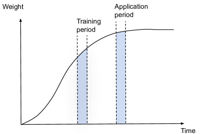
Figure 1: Schematization of the extrapolation capability of the developed tool

The second contribution of our exploration is the development of a concept between the reality and the model (Figure 2). In most cases, the objective of a mathematical model is to translate the reality, adopting a higher or lower abstraction level. In our approach, a differentiation between the reality and our model is made. Indeed, the used support of reflection is not directly the real animal, but an Avatar which conceptually and essentially outlines the global dynamics occurring in the animal body. A large number of physico-chemical phenomena occur in the animal body in response to the ingestion or the injection of molecules. They lead, some time later, to the change of biological variables. This supply of molecules and those biological variables can be monitored and recorded to generate Input and Output data. We assumed that this kind of Inputs and Outputs can be linked by a dynamical model which is a mathematical translation of the Avatar. Therefore, we designed the PDE system mathematically translating our assumption and describing the convection, the diffusion and the action of an overall information flow.

Figure 2: Schematization of the different sets considered in our approach and their own components and processes.

Thirdly, the application of our approach on real data showed that our tool can accurately link biological-related Inputs and Outputs, even if it is fitted on few, scattered and noisy data.

Data-Model Coupling is so far essentially used in the fields of meteorology (see [27]), hydrology (see [28],[29] and [30]), biogeochemistry (see [31], [32], [33] and [34]) and oceanography (see [35]). The successful use of a Data-Model Coupling approach to treat biological issues can be also considered as a contribution of this paper.

In this paper, we will show that the use of a short and relevant PDE system in a fitting process leads to the construction of an efficient predictive tool having a low data dependency and a high information extraction capability.

This tool can be used to predict the evolution of biological variables according to the ingestions and the injections of molecules in the animal body. The objective of the application presented in this paper was to predict the growth of two groups of animals of a specific species, according to their initial weight and their feeding behavior. But the genericity and the parsimony of our tool might ensure its suitability to predict other performance indicators relative to other farm species.

This low data dependency and this high information extraction capability allow the use of few data to fit our tool. Therefore it can be used to reduce the costs relative to experiments, data collection, and data storage. Furthermore, in comparison with the existing predictive tools, these capabilities also make our tool more suitable to efficiently perform Data Assimilation, even if the frequency of data collection and the quality of the collected data are low.

To summarize, in our approach we distinguished different dimensions. As it is illustrated by Figure 3, there is the Reality in which there are Intakes and Injections inducing complex biological processes in the animal body. Some Sensors extract information from this Reality which is stored in databases made of Inputs and Outputs. Since the model is not directly assimilable to the reality, the inflows and the outflows of the model are also not directly assimilable to the input and the output data. The Inputs have to be translated by a mathematical function into Entries, that are pieces of information integrated into the Mathematical Model and that induce the generation of Outcomes, also linked to the Outputs extracted from the Reality by a mathematical function.

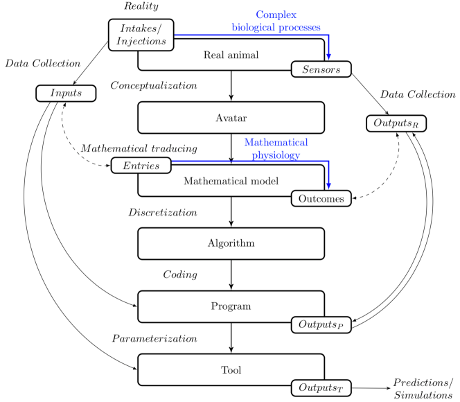
Figure 3: Articulation of the different elements of ourcapabilities exploration

As it can be noticed in Figure 3, our exploration relies on the relationship between several diverse elements such as the Real Animal, the Avatar and the Mathematical Model. The Algorithm comes out of the discretization of the Mathematical Model, e.g. the PDE system which mathematically translates what takes place in the Avatar. This system of PDEs contains parameters corresponding to biological-like factors that can be learned from a database. The $Program$ corresponds to the code that manages this learning step. It uses an iterative training process during which an optimization algorithm finds the values of the parameters that minimize the difference between the measured and the predicted Outputs. The $Tool$ finally corresponds to the Mathematical Model parameterized with the values of the parameters obtained at the end of the learning step.

The presence of parameters that can be learned from data in the mathematical model confers learning ability to the tool based on this model. Using a database, we obtained a tool able to reconstitute dynamics between inputs and outputs to perform forecasts and extrapolations. Hence, the constructed tool can be considered as a Statistical Learning Tool.

In this paper, we will present our modeling approach, the conception of our tool and the results of the applications of our approach on fictitious and real data.

After this Introduction, putting this research work in its proper context, we will detail in Section $2$ the conception of the mathematical model and its applicability.

We tested the well-functioning and the capacities of our tool in two different ways. First, we established a fitting method taking into account the relations existing between the model parameters and we generated a database to test this fitting method on it. This first application on mastered data allowed us to verify the ability of our tool to fit the parameters. Those simulation tests are presented in Section $3$. After those tests on fictitious data, we applied our approach to data collected on a farm and relative to the feeding behavior and the growth of two groups of animals. The results are presented in Section $4$. This application demonstrated the prediction capability of the tool in real conditions.

We put in evidence the potential of our tool and the improvement conferred by it. To do so, we compared the capabilities of our tool with the ones of some Logistic Models, Mechanistic Models and Machine Learning algorithms. These comparisons will be detailed in Section $5$.

2 Construction and description of the Mathematical Model

In our approach, particular attention was paid to the construction of the Mathematical Model embedded in the final predictive tool. Indeed, the designing of this model - that is a PDE system - was the key element to achieve our objectives of lightness, accuracy and learning potency.

2.1 Conception of the Mathematical Model

Through the conceptualization of the Avatar, we set up a parsimonious summary of any biological process. Indeed, we mathematically summarized the global intern dynamics of the animal via several equations and mathematical operators which we assumed necessary and sufficient.

We hypothesized that, when a molecule or a group of molecules enter the body of a living organism, it circulates in the body through a network of vessels containing a fluid. It integrates this fluid and uses it as a vector to evolve via convection and diffusion mechanisms. In the network of vessels, the molecules may be in competition with other mechanisms which may delay its progression. The circulating molecules may then be captured and accumulated in an organ or a specific tissue. During its storage, the molecules can be used and induce a change in some biological variables. Then, we built the PDE system which mathematically translates the previously set up summary illustrated by Figure 4.

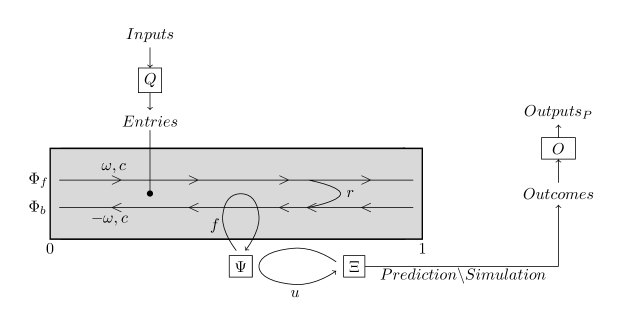
Figure 4: Schematization of the Mathematical Model

We modeled our Avatar using variables, densities, and fields that are all unitless and dimensionless. We also reduced the considered geometrical space to interval $\left[0~{};1\right]$. We considered a Forward Flow $\Phi_{f}$, and a Backward Flow $\Phi_{b}$ streaming in this one-dimensional geometrical space. As it was described in the introduction, these flows can be seen as a very synthetic summary of blood circulation, a circulation in the nervous system or circulation in the digestive tract, according to the problematic.

The involved Inputs in our tool can correspond to collected data relative to feed intakes, water intakes, and administered drugs. These Inputs are integrated in the Mathematical Model via a function $Q$ transforming these Inputs into information inflows, called Entries. We modeled that part of the injected information circulates in a forward direction, via $\Phi_{f}$ and the rest circulates backward, via $\Phi_{b}$. This information can evolve via convection and diffusion phenomena. We assumed that the circulating information can be delayed, captured, stored and used to ultimately induce a modification in the Outcomes $O$. These Outcomes correspond to the model outflows. Those Outcomes are transformed by a mathematical function to be comparable with collected outputs.
Therefore, $\Phi_{\!f}\!(t,x)$ and $\Phi_{b}\!(t,x)$ are, at each instant $t$, two space densities respectively associated with a forward flux with a velocity $\omega$ and a backward flux with a velocity $-\omega$.

The spatial density $\Phi_{\!f}\!(t,x)$ is supposed to be solution to:

$$\frac{\displaystyle\partial\Phi_{\!f}}{\partial t}(t,x)+\omega\frac{\displaystyle\partial\Phi_{\!f}}{\partial x}(t,x)-c\frac{\displaystyle\partial\bigg{[}\chi\frac{\displaystyle\partial\Big{[}\Phi_{\!f}+\Phi_{b}\Big{]}}{\partial x}\bigg{]}}{\partial x}(t,x)~{}\\ =\frac{1}{2}Q(t,x)-fF(x)\Phi_{\!f}(t,x)-r\Phi_{\!f}(t,x),$$ (1)

Similarly, $\Phi_{b}(t,x)$ is supposed to be solution to:

$$\frac{\partial\Phi_{b}}{\partial t}(t,x)-\omega\frac{\displaystyle\partial\Phi_{b}}{\partial x}(t,x)-c\frac{\displaystyle\partial\bigg{[}\chi\frac{\displaystyle\partial\Big{[}\Phi_{\!f}+\Phi_{b}\Big{]}}{\partial x}\bigg{]}}{\partial x}(t,x)~{}\\ =\frac{1}{2}Q(t,x)-fF(x)\Phi_{b}(t,x)+r\Phi_{\!f}(t,x),$$ (2)

In these equations, the parameter $c$ is the diffusion velocity of the information. The space-time density $Q$, corresponds to an external source of information. The function $F$ is worth $0$ in certain areas of the involved geometrical space and $1$ in others. The area where this function is worth $1$ corresponds to the location of the entity capturing the information. The parameter $f$ determines the rate of fixed information. The parameter $r$ determines the fraction of the circulating information transferred from the Forward Flow to the Backward Flow, which induces a delay in the progression of the information.
The function $\chi$ is compactly supported in $(0,1)$, mainly constant and worthing $1$. This function integrated into the diffusion term makes diffusion vanish at the edges of the domain. At each time $t$, the spatial density $\Psi(t,x)$, associated with the fixed information, is solution to:

$$\frac{\partial\Psi}{\partial t}(t,x)=fF(x)\bigg{[}\Phi_{b}(t,x)+\Phi_{\!f}(t,x)\bigg{]}-u\Psi(t,x).$$ (3)

The parameter $u$ is the coefficient determining the usage rate of the fixed information. At each time $t$, the spatial density $\Xi(t,x)$, associated with the used information, is solution to:

$$\frac{\partial\Xi}{\partial t}(t,x)=u\Psi(t,x).$$ (4)

The parameter $\Omega$ corresponds to the area of action of the circulating information on the Outcome. $O(t)$ is the Outcome of the model, given by:

$$O(t)=\int_{\Omega}\Xi(t,x)\,dx.$$ (5)

In this mathematical model we imposed :

$$\forall t\in(0,+\infty),~{}\Phi_{\!f}(t,0)=\Phi_{b}(t,0)\text{ and }\Phi_{b}(t,1)=\Phi_{\!f}(t,1)$$ (6)

These conditions allow the circulating information to move back and forth between the two edges of the domain.

The initial conditions $\Phi_{\!f}(0,x)$, $\Phi_{b}(0,x)$, $\Psi(0,x)$, $\Xi(0,x)$ and $O(0)$ are given for all $x$ in $(0,1)$.

2.2 Applicability of the mathematical model and its different versions

The previously presented mathematical model made of Equations (1), (2), (3), (4) and (5) can be used to simulate and predict an accumulative process. Hence, it can be used to study data relative to a total production over a given period.

The fourth equation of the model is the <<usage>> equation. This equation determines the action of the injected information on the variable to predict. Therefore, this equation has to adapt the different ways in which an intake or an injection may affect a biological variable.
To model a logistical growth, we added a limiter in this equation. In this case, the <<usage>> equation becomes:

$$\frac{\partial\Xi}{\partial t}(t,x)=u\Psi(t,x)\left(\frac{L-O(t)}{L}\right)$$ (4b)

With this version of the equation, data related to the change in weight of an animal can be tackled. This equation is essentially the differential equation of Verhulst [36]:

$$\frac{\partial y}{\partial t}(t)=r~{}y(t)\left(\frac{K-y(t)}{K}\right)$$ (7)

whose structure is equivalent. Indeed, in the case when nothing depends on $x$, the value of $u$ is very high and $\Omega$ is the whole interval $[0~{};~{}1]$, $\Xi$, $\Psi$ and $O$ are very similar. Hence, Equations (7) and (4b) are essentially the same.

It may be also necessary to model variations to use our tool to treat, for example, data concerning drug effects. To do so, we have to be able to model an increase or a decrease in the Outcomes. Since it is the case of most biological variables, we assumed that these outcomes may vary between an upper and a lower bound. Hence, we built two other equations: The equation,

$$\displaystyle\frac{\partial\Xi}{\partial t}(t,x)=-\Big{(}\Xi(t,x)-Upp\Big{)}-u\Psi(t,x)\Big{(}\Xi(t,x)-Low\Big{)}$$ (4c)

models that the fixed information $\Psi$ orients the Outcomes $O$ toward a state that is lower than the steady state, and the equation,

$$\displaystyle\frac{\partial\Xi}{\partial t}(t,x)=-u\Psi(t,x)\Big{(}\Xi(t,x)-Upp\Big{)}-\Big{(}\Xi(t,x)-Low\Big{)}$$ (4d)

models that the fixed information $\Psi$ orients the Outcomes $O$ toward a state which is greater than the steady-state. In these two cases, the Outcomes vary between a lower bound $Low$ and an upper bound $Upp$.

The <<usage>> equation has to be defined a priori according to the variable to predict and the used inputs.

We expect that the mathematical models made of Equations (1), (2), (3), (5) and Equations (4), 4b, 4c or 4d are sufficiently generic to be fitted on data relative to all the different farm species.

2.3 Mesh and discretization of the Mathematical Model

For the discretization of the Mathematical Model, we first used the classical Finite Difference method, with a given space step, to obtain semi-discrete in space equations. And, because the Mathematical Model is coded using R software, we used the R-function $Ode.1D$ developed by Soetaert et al. [37] to manage the temporal discretization of the semi-discrete equations. This R-function calls upon the fourth-order Runge Kutta method with a given time step (See [38]).
In this first exploration, to find a compromise between precision and calculation time, we parameterized the mesh with a time step of $0.001$ and a space step of $0.025$.

2.4 The model parameters

The system of PDEs contains several parameters : $\omega$, $c$, $r$, $f$, $u$ and $L$. The diffusion parameter $c$ is the less influent model parameter. Hence, we set it to $0.001$. All the other parameters are fitted from a database by using an optimization algorithm. To do so, we used the function $directL$ developed by Johnson [39], which is embedded in R ([40]) and applying the DIRECT algorithm developed by Finkel [41]. This algorithm searches the optimal values of the parameters, that is the values that minimize the error associated with the model on a given training database.

A detailed mathematical analysis of the model and its discretization will be performed in an upcoming paper. Nevertheless, we already know that the convection and diffusion speeds must follow the CFL conditions (See [42] and [43]). Indeed, since we set the discretization steps (Section 2.3), $\omega$ must be smaller than $25$ and $c$ must be smaller than $0.625$.

To fit the model we have to specify lower and upper values for each parameter between which the optimization algorithm will search their optimal values. Therefore, a comprehensive study of the ranges of values of the different model parameters was performed and presented in the working paper [44]. We refer to it for the details of this study.

3 Simulation tests of the learning capability of the model

The objective of this section is to present the tests by simulation performed to verify the ability of the tool to learn parameters from noisy biological data. To do so, we started by generating a fictitious database from the parameterized mathematical model made of Equations (1), (2), (3), (4) and (5). Then, we used this database to study the compensation effects existing between the parameters, to simulate the fitting of the parameters and then to verify if the model fits the data correctly.

3.1 Generation of a fictitious database

We generated a fictitious database containing 50 individuals, which is 50 $Output~{}Curves$. The objective was to obtain a database having the same characteristics as a real field database. To do so, we integrated noise and individual variations in it.

The construction of this fictitious database is presented in Appendix I. We refer to it for the details.

Figure 13 shows an example of the generated curves without and with noise. We divided the obtained database into two parts: A Training Database made of $30$ curves and a Test Database made of $20$ curves.

In the rest of this section, we supposed that we have an experimental-like database and a model containing four parameter values to determine: $\omega$, $c$, $r$, $f$ and $u$.

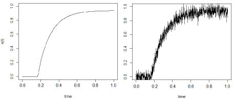
Figure 5: Example of simulated curves without and with noise

3.2 Construction of relations linking some parameters

A study of the compensation effects existing between $\omega$ and $r$ and between $f$ and $u$, put in evidence the existence of relations existing between these two pairs of parameters. For example, the relation existing between the parameters $f$ and $u$ can be noticed in Figure (6).

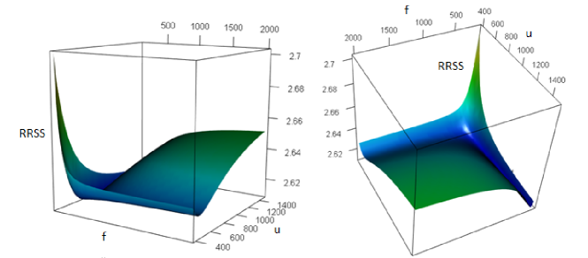
Figure 6: The $3D$ representation of the value of an error indicator (the Relative Residual Sum of Squares). This value is calculating according to the values of $f$ and $u$.

This study is presented in Appendix II. We refer to it for the details.

We concluded from this study that, using a Nadaraya-Watson kernel regressions (See [45] and [46]), we obtained a non-parametric relationship linking $\omega$ and $r$ in the form of,

$$r=\hat{m_{\omega}}(\omega)+\epsilon_{\omega},$$ (8)

and another one linking $f$ and $u$ in the form of,

$$u=\hat{m_{f}}(f)+\epsilon_{f},$$ (9)

where $\hat{m_{\omega}}$ and $\hat{m_{f}}$ corresponds to the Nadaraya-Watson estimators and $\epsilon_{\omega}$ and $\epsilon_{f}$ are the residuals.

Knowing the relationship existing between $\omega$ and $r$ and the one existing between $f$ and $u$ , it is possible to fit $\omega$ and $f$ and then deduce the values of $r$ and $u$. Hence, these relations permits to reduce the number of parameters to learn simultaneously and so facilitate and reinforce the fitting process.

3.3 Parameter fitting and calculation of the model accuracy

We fitted the parameters to the Training Database and then we tested the accuracy of the obtained model by calculating the error made on the Test Database.

3.3.1 Fitting of $\omega$ and $f$ and accuracy of the obtained predictive tool

To perform several fittings we sampled the Training Database: we sampled $20$ curves from the $30$ curves of the Training Database and we fitted the parameters to the $20$ sampled curves. By proceeding in this manner, we performed $30$ fittings of the parameters. To determine the values of $\omega$, $r$, $f$ and $u$, we fitted $\omega$ and $f$ on the selected curves of the Training Database and we deduced the values of $r$ and $u$ using Equalities (8) and (9).

To optimize the parameters, we used the R-function $directl$ to find the values of $\omega$ and $f$ minimizing the function,

$$\displaystyle{f_{obj}(\omega,f)=\frac{1}{n}\sum\limits_{i=1}^{n}\left(\sum\limits_{j=1}^{m}\left(\frac{(y_{ij_{obs}}-y_{ij_{pred}}(\omega,f))}{y_{ij_{obs}}}\right)^{2}\right)}.$$ (10)

After the $30$ fittings of the parameters, we obtained $30$ values of $\omega$, $r$, $f$ and $u$. We calculated the average value and the Relative Standard Deviation (RSD) of each parameter (Table 1). We also looked at the fit of the model calculating from the Training Database the value of the Determination Coefficient ($R^{2}$) (Figure 7 and Table 1). The results show that the model fits the curves of the Training Database well.

Figure 7: Examples of results given by the predictive tool in comparison with some training curves.

Table 1: Average and Relative Standard Deviation of the parameters and the Determination Coefficient calculated on the Training Database.

Parameter	Average	Relative standard deviation
$\omega$	$9.9$	$0.009$
$f$	$920.3$	$0.001$
$r$	$35.6$	$0.016$
$u$	$139.5$	$0.001$
$R^{2}$	$0.97$	$0.011$

To validate the ability of the tool to learn parameters from noisy data, we calculated the accuracy of the model on the Test Database. To do so, we calculated the Relative Residual Sum of Square ($RRSS$) and the Determination Coefficient associated with each curve contained in the Test Database and we obtained the distributions showed in Figure 8. The $RRSS$ is low and the Determination Coefficient is high, indicating that the model fits the curves of the Test Database well.

We compared the $R^{2}$ and the $RRSS$ associated with the Generator model ($R^{2}_{Gener}$ and $RRSS_{Gener}$) - i.e. the model used to generate the fictitious Database - and the $R^{2}$ and the $RRSS$ associated with the Fitted Model ($R^{2}_{Fit}$ and $RRSS_{Fit}$) (Figure 8 and Table 2). $RRSS_{Fit}$ is low and this value is very similar to the value of $RRSS_{Gener}$. The $R^{2}_{Fit}$ is high and this value is also very similar to the value of $R^{2}_{Gener}$. These indicators thus demonstrate that the model fitting method is highly satisfactory and the error associated with the adjusted model is limited to the amount of noise and individual differences initially integrated into the generated database.

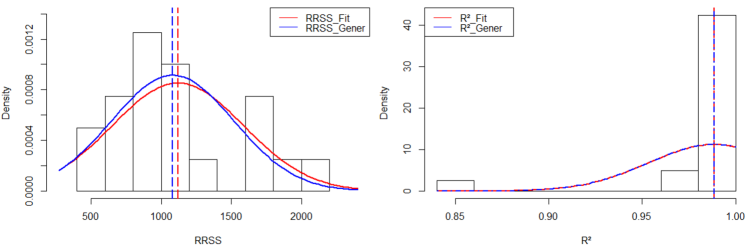
Figure 8: Distributions of the $RRSS$ and of the $R^{2}$ coefficient associated with the $Generator$ $Model$ and the Fitted Model.

Table 2: Comparison between the indicators associated with the Generator Model and the Fitted Model.

	$RRSS$	$R^{2}$
Generator Model	$1082$	$0.9887$
Fitted Model	$1119$	$0.9886$

4 Application of our Biomimetic Statistical Learning Tool on field data

In this section, we present an application of our approach to field data. The database we used is confidential therefore only the dimensionless Inputs and Outputs are presented.

4.1 Objectives of this application on field data

The objective of this application is to build a tool that can predict the logistic growth of animals according to their initial weights and their intakes all along a given period.

4.2 Adaptation of the basic model

To mimic a logistic behavior, we used Equation (4b) as <<usage>> equation (Section 2.2). In this equation, $L$ corresponds to the maximum weight attainable by the animals of the studied species. Experts have an idea of the value of $L$. Therefore, during the model fitting, the value of this parameter was search in a restricted range of values.

Therefore, in this application we used the mathematical model made of Equations (1), (2), (3), (4b) and (5). This model considered as a growth model contained five parameters to fit: $\omega$, $r$, $f$, $u$ and $L$.

4.3 The data used

The database we used is made of two parts corresponding to two different groups of animals monitored during two different periods (Table 3). The first group contained $8$ individuals, monitored over a unit-period from $t=0$ until $t=1$. For this group, the weight of the animals was measured at $t=0$ and at $t=1$. The second group contained $7$ individuals, monitored from $t=0$ until $t=2.5$. For this group the weight of the animals was measured at $t=0$, $t=0.6$, $t=1.52$ and at $t=2.5$. For both groups, intakes of each individual were recorded over each time-step of $0.16$ time-unit. Therefore, for each individual, information relative to those intakes are periodically injected in the model with a time-step of $0.16$.

The dataset relative to the first group constitutes our Training Database and the dataset relative to the second group constitutes our Test Database.

Table 3: Description of the data used.

	First group	Second group
Number of individuals	$8$	$7$
	$t=0$	$t=0$
Output measured at	$t=1$	$t=0.60$
		$t=1.52$
		$t=2.50$
Time step of the Entries injections	$\Delta t_{In}=0.16$	$\Delta t_{In}=0.16$

4.4 Parameter fitting

As in Section 3.2 and Appendix II, we built a relationships between some parameters of the model by applying the same methodology. Using a Nadaraya-Watson kernel regressions, we obtained a non-parametric relation linking $\omega$ and $r$ and another one linking $f$ and $u$. Knowing the relationships between these parameters, it is possible to fit $\omega$ and $f$ and then deduce the value of $r$ and $u$. Therefore in this application we only fitted $\omega$, $f$ and $L$ and deduced the values of $r$ and $u$.

The parameters were fitted to the Training Database by minimizing the difference between the simulated and the real Outputs at time $t=1$. Hence, to fit the parameters, we used the algorithm DIRECT that minimized the function,

$$f_{obj}(\omega,f,L)=\frac{1}{n}\sum\limits_{i=1}^{n}\left(\frac{(s_{i_{obs}}(1)-s_{j_{pred}}(1))}{s_{i_{obs}}(1)}\right)^{2},$$ (11)

where $n$ is the number of individuals contained in the training database and $O_{i_{obs}}(1)$ and $O_{i_{pred}}(1)$ correspond respectively to the values of the observed and the predicted Outputs values for the $i^{th}$ individual at $t=1$.

To performed several fitting procedures. We sampled the Training Database: we randomly selected $7$ individuals from the $8$ individuals before each fitting procedure and we fitted the parameters on the data associated with the selected individuals. Therefore, we performed $8$ fittings and we obtained $8$ sets of values of $(\omega,r,f,u,L)$.

4.5 Results

We calculated the average and the $RSD$ of each parameter (Table 4). The $RSD$ of each parameter is low, indicating that our fitting method permitted to identify one set containing the parameter values that minimize the error associated with the Fitted Model. The existence of a single optimal set of values of $(\omega,r,f,u,L)$ attests to the identifiability of the model.

We parameterized the model with the average values of the parameters.

We calculated the error associated with the model on the Training Database. To do so, we calculated the Average Relative Error ($ARE$) between the measured and predicted values of the Output at time $t=1$:

$$ARE(t)=\frac{1}{n}\sum\limits_{i=1}^{n}\sqrt{\left(\frac{(s_{i_{obs}}(t)-s_{j_{pred}}(t))}{s_{i_{obs}}(t)}\right)^{2}}$$ (12)

Table 4: Average values and $RSD$ of the fitted parameters. $ARE$ calculated at time $t=1$ on the Training Database.

$Parameter$	$Mean$	$RSD$
$\omega$	$9.24$	$0.079$
$r$	$17.91$	$0.14$
$f$	$707.01$	$0.36$
$u$	$21.49$	$0.17$
$L$	$1.70$	$0.009$
$ARE(1)$ $(\%)$	$1.83$	$0.013$

The $ARE$ value calculated on the Training Database at time $t=1$, is worth $1.83\%$. This result is satisfactory, but the accuracy of the model must be calculated on a Test Database to ensure that the model does not overfit the training data.

To do so, we calculated the $ARE$ given by Equation (12), on the Test Database at time $t=0.6$, $t=1.52$ and $t=2.5$ (Table 5 and Figure 9).

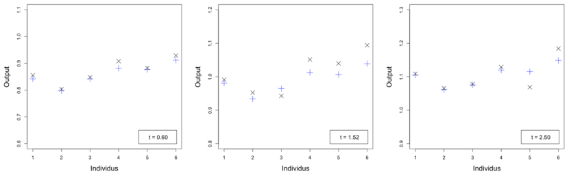
Figure 9: Difference obtained between the measured ($+$) and predicted ($\times$) values of the Output variable at different times $t$ for the individuals in the Test Database.

Table 5: Average Relative Error ($ARE$) calculated on the Test Database at different instants.

t	$0.6$	$1.52$	$2.5$
ARE(t) (%)	$1.3$	$2.9$	$1.5$

4.6 Discussion of the results

The error associated with the model is low on the Test Database. The errors made before and after time $t=1$ remain low. Those results indicate that our tool can be trained on a very small database to link the inputs and the outputs and then it can accurately predict the weight of the animals over a period $2.5$ times longer than the training one.
This extrapolation capability, obtained despite the very low quantity of training data, illustrates that our tools hold high potential for information extraction. As it will be demonstrated below, this capability distinguishes our approach from other inference methods.

Moreover, in addition to the information extraction potential, the extrapolation capability helps to reduce the training-data-dependency of our tool. Indeed, we demonstrated that our tool can be applied outside the training data range and provide accurate extrapolations. Hence, we do not need to fit it on data covering the whole curve to predict and so we can use smaller Training Database. Therefore, this extrapolation capability permits to reduce the duration of data collection, the duration of in situ experiments, and thus the computational and the experimental costs.

5 Comparison with existing growth models

According to [16] and [47], the current methods used to simulate and predict logistic growth processes, involve two main types of models: Phenomenological Models corresponding to <<Black Box>> models, and Mechanistic Models corresponding to <<White Box>> models. In this section, we will compare some models belonging to these two main categories with the Biomimetic Statistical Learning tool presented in this paper.

5.1 The Phenomenological Models

As defined in [16], the Phenomenological Models include Linear, Multiple Linear and Nonlinear Regressions, Logistic Models and Neuronal Networks.

5.1.1 Comparison of our Biomimetic Growth Model with Classical Logistic Growth Models

The models of Gompertz [48],

$$\frac{dN(t)}{dt}=a_{G}.N(t).\ln\left(\frac{K_{G}}{N(t)}\right),$$ (13)

and Verhulst [36],

$$\frac{dN(t)}{dt}=a_{V}.N(t).\left(1-\frac{N(t)}{K_{V}}\right),$$ (14)

are two models frequently used to model growth processes (e.g. see [49], [50], [51], [52], [53] and [54]).
We fitted the parameters of these two models on our Training Database by using the same optimization algorithm that we used to fit the Biomimetic Model and by minimizing $ARE(1)$.

To test and compare the accuracy of the different models, we calculated on the Test Database the Average Relative Accuracy, $ARA$ at different times $t$ :

$$ARA(t)=1-ARE(t),$$ (15)

where $ARE$ is given by Equation (12). We used the three parameterized models to generate the growth curve of the individuals of the Test Database and we compared the measured and the predicted values at times $t=0.6$, $t=1.52$ and $t=2.5$.
The results contained in Table 6 and the curves of Figures 10 and 11 show that the curves generated from the Gompertz’s model featured a premature deceleration. However, the Verhulst’s model is associated with good accuracy over the whole studied period.

The similarity of the results from the Verhulst and the Biomimetic Growth Models was expected because our model includes an equation assimilable to the Verhulst’s equation (see Section 2.2). The real advantage of our biomimetic growth model is its ability to integrate input data. Indeed, the Verhulst equation only takes into account the initial conditions of the system under study, whereas our model also integrates intakes throughout the studied period. The capability to integrate additional information appears to help refine the results and increase the accuracy of our model. Moreover, since the Verhulst’s and the Gompertz’s models can not integrate input data over time, they are not able to perform Data Assimilation, contrary to our tool.

Table 6: Parameter values and $ARA(1)$ calculated on the Training Database.

Model	a	K	ARA(1)
Gompertz	$a_{G}=0.412$	$K_{G}=0.563$	$0.978$
Verhulst	$a_{V}=0.411$	$K_{V}=1.563$	$0.979$
Biomimetic			$0.981$

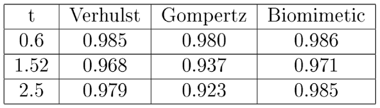
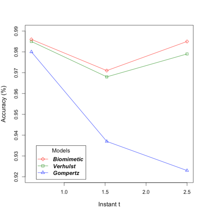
Figure 10: The $ARA$ calculated on the Test Database at different times $t$ and associated with different models.

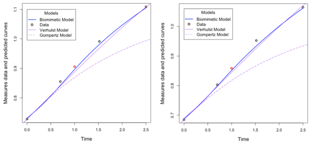
Figure 11: Plot of the predicted growth curves of two individuals contained in the Test Database with the different models.

5.1.2 Comparison between the Biomimetic Growth Model and Neural Networks

Over the past decade, the use of Machine Learning (ML) algorithms and especially Neural Networks (NN) has been on the rise [55]. According to some studies ([56], [57], [58] and [59]), the popularity of these tools can be explained by the ease of their implementation and the diversity of issues that these algorithms can handle. Nevertheless, these algorithms are based on relatively simple mathematical models that are cannot easily take into account complex phenomena, such as delay and saturation. Hence, we applied different Neural Networks on our Training Database to compare this kind of ML tool and our Biomimetic Growth Model. We tested six Neural Networks having different numbers of nodes and hidden layers, taken as inputs the initial weight of each individual and their periodically recorded intakes (Table 7).

Table 7: The $ARA$ calculated on the Training Database ($ARA_{Train}$), and on the Test Database ($ARA_{Test}$), at $t=1$, with different Neural Networks. The Neural Network ($k_{1}$,…,$k_{i}$,…,$k_{n}$) corresponds to a Neural Network containing $n$ hidden layers and the $i^{th}$ hidden layer contains $k_{i}$ nodes.

Structure	$ARA_{Train}(1)$ ($\%$)	$ARA_{Test}(1)$ ($\%$)
(4)	99.9	78.8
(4,3)	99.8	90.5
(6,5)	99.7	93.4
(4,6,6,3)	99.9	94.8
(5,7,7,7,4)	99.8	95.3
(5,9,9,9,5)	99.9	93

We fitted each tested Neural Network on our Training Database by using the R-function $neuralnet$ developed by Fritsch et al. [60], and we calculated the accuracy of those Neural Networks on the $Training$ and on the Test Database.

The results given in Table 7 show that all the tested Neural Network fit the curves of the Training Database better than the ones of the Test Database. It shows that the tested Neural Network overfit the training curves, particularly when the structure of the studied Neural Networks is composed of too many or too few nodes and hidden layers. The accuracy of the Neural Networks on the Test Database increases up to a certain number of nodes and hidden layers and then decreases when the complexity of the structure continues to increase. On the test database, the highest accuracy value is reached using a Neural Networks containing $5$ hidden layers, but this value is lower than that obtained using our Biomimetic Model (Table 7 and Figure 10).

Nevertheless, the accuracy of these ML tools is satisfactory and the real advantage of our Biomimetic tool over Neural Networks is its extrapolation capability. Indeed, as the Biomimetic Model, the studied Neural Networks were fitted only from the value of the Output at $t=1$. In this case, the fitted classical Neural Networks can only be used to predict the Output at $t=1$. Hence, Neural Networks cannot interpolate or extrapolate, in contrast to our Biomimetic Model. Therefore, contrary to our tool, Neural Networks can not be used in a "Biological Small Data" context to reduce the experimental and computational costs. They are also less suitable to perform Data Assimilation in this context.

5.2 Mechanistic Growth Models

Mechanistic Growth Models are another kind of tool permitting to gathered biological inputs to predict the growth of plants or animals. Some models of this type have been developed in [61], [62], [63] and [64]. These models integrate numerous Inputs, and not all of which are available in our study. Hence, these models can not be applied to our database. Therefore, we only compared the structure, the functioning and the objectives of those Mechanistic Models with our Biomimetic one.

As it is said in [16], [65], [17] and [66], the construction of Mechanistic Growth Models generally focuses on the biological meaning of the overall model. Therefore, the construction of the explanatory mechanistic models takes time, requires a large quantity of zootechnical knowledge and results in complex models. As it is explained in [67], [17] and [68], these models contain a large number of unknown parameters and include many factors, forcing the user to enter a large number of Input values, which are sometimes difficult or costly to obtain. Hence, the complex structure of these models makes Mechanistic Realistic Models inappropriate for fitting data and Data Assimilation.

6 Conclusion

To conclude, we built a Biomimetic Statistical Learning tool based on a PDE system embedding the mathematical expression of biological determinants. This PDE system contains parameters that can be fitted to data. This PDE system was carefully designed to have a high learning potency and a great accuracy but also to remain light and flexible.

In the particular <<Biological Small Data>> context, the performed applications showed that this tool has higher accuracy than the existing tools. However, our Biomimetic Statistical Learning tool distinguishes itself in light of its suitability to perform Data Assimilation even if the frequency of data collection and the quality of the collected data are low.
The extrapolation capability of our tool, coupled with its high learning potency permits to fit it on a few data but also to accurately applied it outside the range of the training data. Hence, the quantity of collected data can be reduced as the costs relative to experiments and data management.

To sum up, our tool can be used to predict health and performance indicators according to the ingestion or the injection of molecules in an animal body and to perform accurate and inexpensive Livestock Data Assimilation .
The pursuit of an optimal combination between the use of data and the use of prior knowledge via the use of PDEs seems to be an interesting way to build Artificial Intelligence (AI) tools. Those AI tools could have a strong learning ability and a weak Training-Data-Dependency.

Nevertheless, the results coming from the Biomimetic Model was obtained from a certain number of hypotheses. Some Model Selection methods could be applied to select the structure of the Mathematical Model, permitting to obtain a more satisfying model in terms of $ARE$ and the number of parameters to learn. This suggested improvement will be studied in a forthcoming work.

Appendix I: Generation of the Learning Database

To test the learning capability of the model we generated a Learning Database containing 50 individuals, that is 50 $Output~{}Curves$. The objective is to obtain a database having the same characteristics as a real field database. To do that we integrated into this fictitious database noise and individual variability.

I.1 Integration of individual variability

The model parameters are constants to determine. Nevertheless, to introduce individual variability in the generated data, we considered (only in this Section) the parameters as biological-like factors following a Normal distribution. To simulate individual differences, we assigned to each parameter a Normal distribution centered on an arbitrarily chosen value and with a relative variance of $0.005$ (See Table 8). From these Normal probability laws, we generated $50$ values of the parameters $\omega$, $r$, $f$ and $u$. Their respective statistical and probabilistic distributions are given in Figure 12.

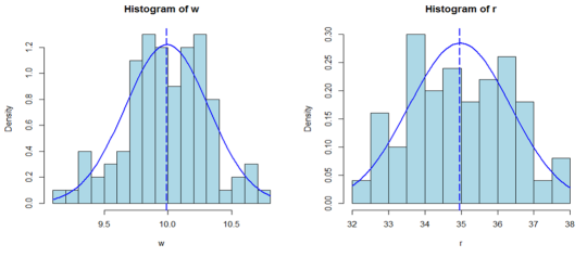
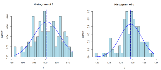
Figure 12: Distributions of the parameters $\omega$, $r$, $f$ and $u$

I.2 Generation of fictitious Inputs

The $Inputs$ integrated into the model correspond to the injected volume ($VolQ$) and the moment of the injection ($c_{t}$). These parameters can take on any value between $0$ and $1$, therefore we applied a Uniform distribution over the interval $[0;1]$ to these two types of $Inputs$ (Table 8).

From the values of the parameters and the fictitious $Inputs$, we generated $50$ $Output~{}Curves$.

I.3 Addition of a random noise

Continuing with the objective of obtaining an experimental-like database, we added noise to the $Output~{}Curves$. To do so, we added a random component following a Gaussian distribution centered on $0$ and with a variance of $0.05$ to the generated curves (Table 8).

Figure 13 shows some examples of generated curves without and with noise. We divided the obtained database into two datasets: A $Training~{}Database$ made of $30$ curves and a $Test~{}Database$ made of $20$ curves.

In the rest of this Section, we assumed that we have an experimental-like database and a model containing four parameter values to determine.

Table 8: The distributions followed by the parameters and the $Inputs$.

Parameter	Probability law
$\omega$	$\mathcal{N}(10,0.3125)$
$r$	$\mathcal{N}(35,1.42)$
$f$	$\mathcal{N}(800,5.175)$
$u$	$\mathcal{N}(125,1)$
$VolQ$	$\mathcal{U}(0,1)$
$c_{t}$	$\mathcal{U}(0,1)$
$Noise$	$\mathcal{N}(0,0.05)$

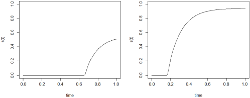
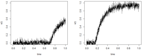
Figure 13: Example of simulated curves without and with noise

Appendix II: Study of the compensation effects existing between the model parameters

Among the parameters $\omega$, $r$, $f$ and $u$, some parameters offset each other.

Velocity $\omega$, can be offset by any delay $r$, the information undergoes. For example, a low convection speed associated with a low delay may induce kinetics equivalent to that induced by a high convection speed associated with a long delay.

The fixation $f$, and the use of the information $u$, are also two counterbalanced processes. For instance, a high fixation rate followed by a low usage of the information can induce the same effect on the $Outcome$ as a low fixation rate followed by an important use of the fixed information.

Therefore, relations exist between the parameters of those two couples. The objective of this part is to use the fictitious $Training~{}Database$ to study these relations.

II.1 Study of the relationship between $\omega$ and $r$

First, we demonstrated the relationship existing between $\omega$ and $r$ by calculating the error made on the $Training~{}Database$ by the model parametrized with different $(\omega,r)$ pairs. To do so, we ranged the domain $\omega\times r$ and we calculated the Relative Residual Sum of Squares ($RRSS$) (16) associated with the models parametrized with different tested $(\omega,r)$ pairs:

$$\displaystyle{RRSS(\omega,r)=\sum\limits_{i=1}^{n}\left(\sum\limits_{j=1}^{m}\left(\frac{(y_{ij_{obs}}-y_{ij_{pred}}(\omega,r))}{y_{ij_{obs}}}\right)^{2}\right)},$$ (16)

where $n$ corresponds to the number of individuals contained in the $Training~{}Database$ and $m$ the number of points on the curves. $y_{ij_{obs}}$ and $y_{ij_{pred}}$ correspond respectively to the observed and the predicted value of the $j^{th}$ point of the $i^{th}$ individual. Therefore $RRSS$ corresponds to the sum of the squared relative differences between the predicted curves and the initially generated curves.

Figures 14 and 15 give the values of the RRSS according to the values of $\omega$ and $r$. The existence of a series of equivalent pairs - that is a series of pairs leading to the same value of $RRSS$ - can be seen in Figure 14(a). There is an area where the $RRSS$ values are lower (Figure 15), and corresponding to the curve $EC1$ in Figure 14(b). We assumed that the optimal ($\omega_{{Opt}}$,$r_{{Opt}}$) pair, inducing the lowest RRSS, belongs to this curve. Therefore, we set out to determine the equation of the curve $EC1$.

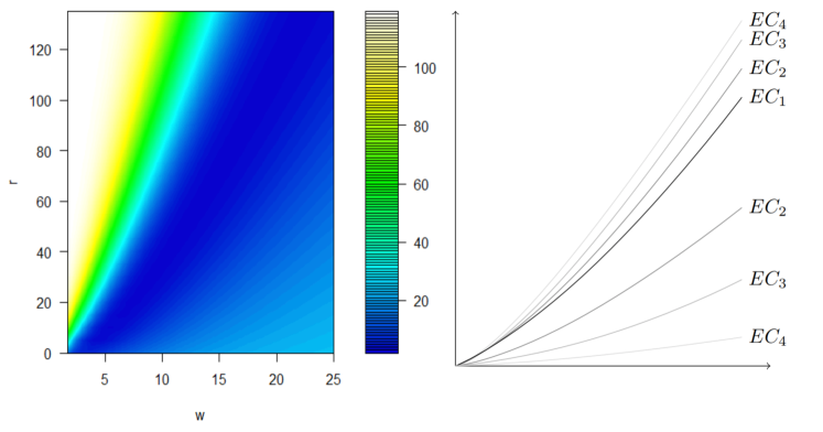
Figure 14: The value of the $RRSS$ according to $\omega$ and $r$ (a: left), and the schema of the different Equivalent Couples (EC) (b: right)

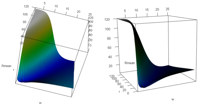
Figure 15: The $3D$ representation of the value of the $RRSS$ according to $\omega$ and $r$

II.2 Search for the $(\omega_{{Opt}},r_{{Opt}})$ pairs inducing the lowest $RRSS$

To find the equation of the curve $EC1$ we sought for different values of $\omega$, the value of $r$ minimizing the $RRSS$ value. To do that, for each tested value of $\omega$ we used the optimization algorithm DIRECT to find the value of $r$ minimizing the objective function,

$$\displaystyle{f_{obj}(r)=\frac{1}{n}\sum\limits_{i=1}^{n}\left(\sum\limits_{j=1}^{m}\left(\frac{(y_{ij_{obs}}-y_{ij_{pred}}(\omega,r))}{y_{ij_{obs}}}\right)^{2}\right)},$$ (17)

corresponding to the average RRSS.

To obtain several fitted values of $r$ for each tested value of $\omega$, we sampled the $Training~{}Database$: we sampled $20$ curves from the $30$ test curves and we fitted $r$ on those $20$ selected curves. We ultimately obtained three values of $r$ for each tested value of $\omega$ (Figure 16). Using a Nadaraya-Watson kernel regression (See [45] and [46]), we obtained a non-parametric relationship linking $\omega_{{Opt}}$ and $r_{{Opt}}$ in the form of:

$$r_{opt}=\hat{m}(\omega_{opt})+\epsilon,$$ (18)

where $\hat{m}$ corresponds to the Nadaraya-Watson estimator.

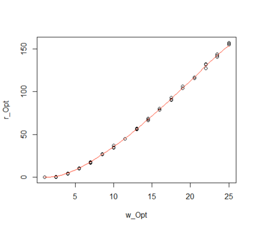
Figure 16: The Nadaraya-Watson kernel regression linking the ($\omega_{{Opt}}$, $r_{{Opt}}$) parameter pair.

Knowing the relationship between $\omega_{{Opt}}$ and $r_{{Opt}}$, it is possible to deduce one of these two parameters according to the value of the other parameter. Hence, this relationship reduces the number of parameters that need to be learned simultaneously.

II.3 Study of the relationship between $f$ and $u$

There is also a compensation effect between $f$ and $u$: a high value of $f$ can be compensated by a low value of $u$, and vice versa.

As above for $\omega$ and $r$, we sought to determine the relationship existing between $f$ and $u$ to be able to deduce one of these two parameters according to the other one and further reduce the number of parameters to learn simultaneously.

As above, we ranged the domain $f\times u$ and calculates the $RRSS$ of the models parameterized with different pairs of values for $(f,u)$ (Figures 17 and 18). This study demonstrates a series of equivalent pairs. There is an area where the $RRSS$ values are lower (Figure 18) and corresponding to the $EC1$ curve in Figure 17(a). We assumed that the optimal $(f_{{Opt}},u_{{Opt}})$ pair inducing the lowest $RRSS$, belongs to this curve. Therefore, we set out to determine the equation of this curve.

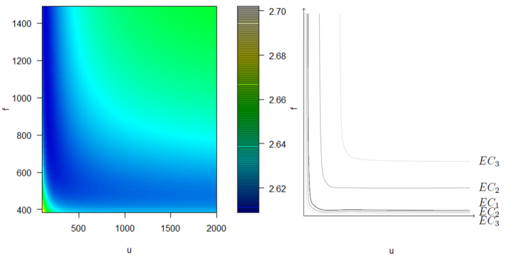
Figure 17: The value of the RRSS according to $f$ and $u$ (a) and the schema of the different Equivalent Couples (EC) (b)

Figure 18: The $3D$ representation of the value of the RRSS according to $f$ and $u$

II.4 Search for the $(f_{{Opt}},u_{{Opt}})$ pairs that lead to the lowest $RRSS$

To find the equation of the curve $EC1$ associated with the lowest $RRSS$, we looked for the value of $u$ minimizing the $RRSS$ value for different given values of $f$. For each value of $f$, we used the optimization algorithm DIRECT to find the value of $u$ minimizing the objective function (19) corresponding to the average $RRSS$.

$$\displaystyle{f_{obj}(u)=\frac{1}{n}\sum\limits_{i=1}^{n}\left(\sum\limits_{j=1}^{m}\left(\frac{(y_{ij_{obs}}-y_{ij_{pred}}(f,u))}{y_{ij_{obs}}}\right)^{2}\right)}.$$ (19)

As above, to obtain several fitted values of $u$ for each tested value of $f$, we sampled the $Training~{}Database$. At the end of the fitting, we obtained three values of $u$ for each tested value of $f$ (Figure 19). Using a Nadaraya-Watson kernel regression, we obtained a non-parametric relationship linking $f_{{Opt}}$ and $u_{{Opt}}$ in the form of:

$$u_{{Opt}}=\hat{m}(f_{{Opt}})+\epsilon,$$ (20)

where $\hat{m}$ corresponds to the Nadaraya-Watson estimator.

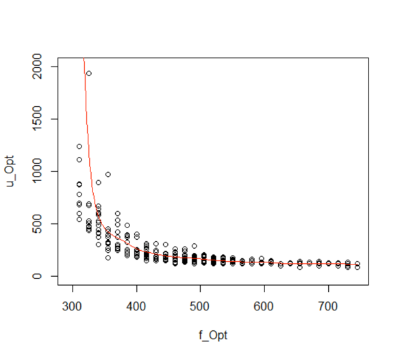
Figure 19: The Nadaraya-Watson kernel regression linking $f_{{Opt}}$ and $u_{{Opt}}$.

Knowing the relationship existing between $f_{{Opt}}$ and $u_{{Opt}}$, it is possible to deduce one of these two parameters according to the value of the other parameter. Hence, this relationship further reduces the number of parameters to learn simultaneously.

References

- [1] M. McPhee “Mathematical modelling in agricultural systems : A case study of modelling fat deposition in beef cattle for research and industry”, 2009
- [2] L. Puillet, O. Martin, D. Sauvant and M. Tichit “Introducing efficiency into the analysis of individual lifetime performance variability: a key to assess herd management” In animal 5.1 Cambridge University Press (CUP), 2011, pp. 123–133 DOI: 10.1017/S175173111000162X
- [3] O. Martin and D. Sauvant “A teleonomic model describing performance (body, milk and intake) during growth and over repeated reproductive cycles throughout the lifespan of dairy cattle. 2. Voluntary intake and energy partitioning” In Animal 4.12 Cambridge University Press, 2010, pp. 2048ñ2056 DOI: 10.1017/S1751731110001369
- [4] J. D. Nkrumah, J. Basarab, Z. Wang, C. Li, M. Price, E. Okine, D. H. Crews and S. S. Moore “Genetic and phenotypic relationships of feed intake and measures of efficiency with growth and carcass merit of beef cattle” In Journal of animal science 85, 2007, pp. 2711–20 DOI: 10.2527/jas.2006-767
- [5] H. Nesetrilova “Multiphasic growth models for cattle” In Czech Journal of Animal Science 50, 2005, pp. 347–354 DOI: 10.17221/4176-CJAS
- [6] J. Basarab, M. Price, J. L. Aalhus, E. Okine, W. M. Snelling and K. L. Lyle “Residual Feed intake and body composition in young growing cattle” In Canadian Journal of Animal Science 83, 2003, pp. 189–204 DOI: 10.4141/A02-065
- [7] D. Auroux and J. Blum “Back and forth nudging algorithm for data assimilation problems” In Comptes Rendus Mathematique 340.12 Elsevier, 2005, pp. 873–878
- [8] W. W. Gregg, M. AM. Friedrichs, A. R. Robinson, K. A. Rose, R. Schlitzer, K. R. Thompson and S. C. Doney “Skill assessment in ocean biological data assimilation” In Journal of Marine Systems 76.1-2 Elsevier, 2009, pp. 16–33
- [9] R. Lguensat, P. Tandeo, P. Ailliot, M. Pulido and R. Fablet “The analog data assimilation” In Monthly Weather Review 145.10, 2017, pp. 4093–4107
- [10] R. Lguensat, P. H. Viet, M. Sun, G. Chen, T. Fenglin, B. Chapron and R. Fablet “Data-driven Interpolation of Sea Level Anomalies using Analog Data Assimilation” In Remote Sensing 11.7 Multidisciplinary Digital Publishing Institute, 2019, pp. 858
- [11] Rui LI, Cun LI, Ying DONG, Feng LIU, Ji WANG, Xiao YANG and Yu PAN “Assimilation of Remote Sensing and Crop Model for LAI Estimation Based on Ensemble Kaiman Filter” In Agricultural Sciences in China 10.10, 2011, pp. 1595 –1602 DOI: https://doi.org/10.1016/S1671-2927(11)60156-9
- [12] Bert Rijk “Integration of sensor data in crop models for precision agriculture”, 2013
- [13] S Janssen, CH Porter, AD Moore, IN Athanasiadis, I Foster, JW Jones and JM Antle “Towards a new generation of agricultural system models, data, and knowledge products: building an open web-based approach to agricultural data, system modeling and decision support. AgMIP” In Towards a New Generation of Agricultural System Models, Data, and Knowledge Products 91, 2015
- [14] J. C. W. Locke, A. J. Millar and M. S. Turner “Modelling genetic networks with noisy and varied experimental data: the circadian clock in Arabidopsis thaliana.” In Journal of theoretical biology 234 3, 2005, pp. 383–93
- [15] Y. Qi, Z. Bar-Joseph and J. Klein-Seetharaman “Evaluation of different biological data and computational classification methods for use in protein interaction prediction” In Proteins: Structure, Function, and Bioinformatics 63.3, 2006, pp. 490–500 DOI: 10.1002/prot.20865
- [16] M. A. Vázquez-Cruz, A. Espinosa-Calderón, A. R. Jiménez-Sánchez and R. Guzmán-Cruz “Mathematical Modeling of Biosystems” In Biosystems Engineering: Biofactories for Food Production in the Century XXI Cham: Springer International Publishing, 2014, pp. 51–76 DOI: 10.1007/978-3-319-03880-3_2
- [17] D. Bastianelli and D. Sauvant “Modelling the mechanisms of pig growth.” In Livestock Production Science, 1997
- [18] O. Martin and D. Sauvant “A teleonomic model describing performance (body, milk and intake) during growth and over repeated reproductive cycles throughout the lifespan of dairy cattle. 1. Trajectories of life function priorities and genetic scaling.” In Animal, 2010
- [19] A. C. Tan and D. Gilbert “An empirical comparison of supervised machine learning techniques in bioinformatics” In Proceedings of the First Asia-Pacific bioinformatics conference on Bioinformatics 2003-Volume 19, 2003, pp. 219–222 Australian Computer Society, Inc.
- [20] J. Shavlik, L. Hunter and D. Searls “Introduction” In Machine Learning 21.1, 1995, pp. 5–9 DOI: 10.1007/BF00993376
- [21] T. Hubbard and A. Reinhardt “Using neural networks for prediction of the subcellular location of proteins” In Nucleic Acids Research 26.9, 1998, pp. 2230–2236 DOI: 10.1093/nar/26.9.2230
- [22] S. H. Dumpala, R. Chakraborty and S. K. Kopparapu “k-FFNN: A priori knowledge infused Feed-forward Neural Networks”, 2017 arXiv:1704.07055 [cs.LG]
- [23] E. Frénod “A PDE-like Toy-Model of Territory Working” In Understanding Interactions in Complex Systems - Toward a Science of Interaction, Understanding Interactions in Complex Systems - Toward a Science of Interaction Cambridge Scholar Publishing, 2017, pp. 37–47 URL: https://hal.archives-ouvertes.fr/hal-00817522
- [24] A. Rousseau and M. Nodet “Modélisation mathématique et assimilation de données pour les sciences de l’environnement” In Bulletin de l’APMED, 2013, pp. 467–472
- [25] W. J. Sacks, D. S. Schimel and R. K. Monson “Coupling between carbon cycling and climate in a high-elevation, subalpine forest: a model-data fusion analysis” In Oecologia 151.1, 2007, pp. 54–68 DOI: 10.1007/s00442-006-0565-2
- [26] L. Wang, H. Zhang, K. C. L. Wong, H. Liu and P. Shi “Physiological-model-constrained noninvasive reconstruction of volumetric myocardial transmembrane potentials” In IEEE Transactions on Biomedical Engineering 57.2 IEEE, 2010, pp. 296–315
- [27] A. J. Simmons and A. Hollingsworth “Some aspects of the improvement in skill of numerical weather prediction” In Quarterly Journal of the Royal Meteorological Society 128.580, 2002, pp. 647–677 DOI: 10.1256/003590002321042135
- [28] G. Kim and A. P. Barros “Space–time characterization of soil moisture from passive microwave remotely sensed imagery and ancillary data” In Remote Sensing of Environment 81.2, 2002, pp. 393 –403 DOI: https://doi.org/10.1016/S0034-4257(02)00014-7
- [29] W. L. Crosson, C. A. Laymon, R. Inguva and M. P. Schamschula “Assimilating remote sensing data in a surface flux–soil moisture model” In Hydrological Processes 16, 2002, pp. 1645–1662 DOI: 10.1002/hyp.1051
- [30] D. S. Mackay, S. Samanta, R. R. Nemani and L. E. Band “Multi-objective parameter estimation for simulating canopy transpiration in forested watersheds” In Journal of Hydrology 277.3, 2003, pp. 230 –247 DOI: https://doi.org/10.1016/S0022-1694(03)00130-6
- [31] D. J. Barrett “Steady state turnover time of carbon in the Australian terrestrial biosphere” In Global Biogeochemical Cycles 16.4, 2002, pp. 55–1–55–21 DOI: 10.1029/2002GB001860
- [32] D. Barrett, M. Hill, L. Hutley, J. Beringer, J. H. Xu, G. Cook, J. Carter and R. J. Williams “Prospects for improving savanna biophysical models by using multiple-constraints model-data assimilation methods” In Australian Journal of Botany 53(7), 2005 DOI: 10.1071/BT04139
- [33] P. J. Rayner, M. Scholze, W. Knorr, T. Kaminski, R. Giering and H. Widmann “Two decades of terrestrial carbon fluxes from a carbon cycle data assimilation system (CCDAS)” In Global Biogeochemical Cycles 19.2, 2005 DOI: 10.1029/2004GB002254
- [34] W. J. Sacks, D. S. Schimel, R. K. Monson and B. H. Braswell “Model-data synthesis of diurnal and seasonal CO2 fluxes at Niwot Ridge, Colorado” In Global Change Biology 12.2, 2006, pp. 240–259 DOI: 10.1111/j.1365-2486.2005.01059.x
- [35] P. Ailliot, E. Frénod and V. Monbet “Long term object drift in the ocean with tide and wind.” In SIAM Journal on Multiscale Modeling and Simulation: A SIAM Interdisciplinary Journal 5 (2), 2006, pp. 514 –531 URL: https://hal.archives-ouvertes.fr/hal-00129093
- [36] P. F. Verhulst “Notice sur la loi que la population suit dans son accroissement” In Corresp. Math. Phys. 10, 1838, pp. 113–126 URL: https://ci.nii.ac.jp/naid/10015246307/en/
- [37] K. Soetaert, T. Petzoldt and R. Woodrow Setzer “Solving Differential Equations in R: Package deSolve” In Journal of Statistical Software 33.9, 2010, pp. 1–25 DOI: 10.18637/jss.v033.i09
- [38] W. Enright “The Numerical Analysis of Ordinary Differential Equations: Runge Kutta and General Linear Methods” In SIAM Review 31.4, 1989, pp. 693–693 DOI: 10.1137/1031147
- [39] S. G. Johnson “The NLopt nonlinear-optimization package”, 2008
- [40] R Core Team “R: A Language and Environment for Statistical Computing”, 2014 R Foundation for Statistical Computing URL: http://www.R-project.org/
- [41] D. E. Finkel “DIRECT Optimization Algorithm” North Carolina State University, 2003
- [42] R. Courant, K. Friedrichs and H. Lewy “Über die partiellen Differenzengleichungen der mathematischen Physik” In Mathematische annalen 100.1 Springer, 1928, pp. 32–74
- [43] E. W. Weisstein “Courant-friedrichs-lewy condition” In Wolfram MathWorld–A Wolfram Web Resource., 2014
- [44] H. Flourent “Study of the ranges of values of a Biomimetic Statistical Learning Tool parameters” Working paper, 2019 URL: https://hal.archives-ouvertes.fr/hal-02067374
- [45] E. A. Nadaraya “On estimating regression” In Theory of Probability & Its Applications 9.1 SIAM, 1964, pp. 141–142
- [46] G. S. Watson “Smooth regression analysis” In Sankhyā: The Indian Journal of Statistics, Series A JSTOR, 1964, pp. 359–372
- [47] R. Guzmán-Cruz, R. Castaneda-Miranda, J. Garcia-Escalante, L. Solis-Sánchez, D. Alaniz-Lumbreras, J. Mendoza-Jasso, A. Lara-Herrera, G. Ornelas-Vargas, E. Gonzalez-Ramirez and R. Montoya-Zamora “Evolutionary Algorithms in Modelling of Biosystems”, 2011 DOI: 10.5772/16231
- [48] B. Gompertz “XXIV. On the nature of the function expressive of the law of human mortality, and on a new mode of determining the value of life contingencies. In a letter to Francis Baily, Esq. FRS &c” In Philosophical transactions of the Royal Society of London 115 The Royal Society, 1825, pp. 513–583
- [49] C. P. Winsor “The Gompertz Curve as a Growth Curve” In Proceedings of the National Academy of Sciences 18.1 National Academy of Sciences, 1932, pp. 1–8 DOI: 10.1073/pnas.18.1.1
- [50] N. K. Sakomura, F. A. Longo, E. O. Oviedo-Rondon, C. Boa-Viagem and A. Ferraudo “Modeling energy utilization and growth parameter description for broiler chickens” In Poultry Science 84.9 Oxford University Press Oxford, UK, 2005, pp. 1363–1369
- [51] J. Buyse, B. Geypens, R. D. Malheiros, V. M. Moraes, Q. Swennen and E. Decuypere “Assessment of age-related glucose oxidation rates of broiler chickens by using stable isotopes” In Life sciences 75.18 Elsevier, 2004, pp. 2245–2255
- [52] T. B. Robertson “Experimental studies on growth II. The normal growth of the white mouse” In Journal of Biological Chemistry 24.3 ASBMB, 1916, pp. 363–383
- [53] T. B. Robertson “The chemical basis of growth and senescence” JB Lippincott Company, 1923
- [54] P. Román-Román and F. Torres-Ruiz “Modelling logistic growth by a new diffusion process: Application to biological systems” In Biosystems 110.1 Elsevier, 2012, pp. 9–21
- [55] P. Domingos “A Few Useful Things to Know About Machine Learning” In Commun. ACM 55, 2012, pp. 78–87 DOI: 10.1145/2347736.2347755
- [56] M. T. Gorczyca, H. F. M. Milan, A. S. C. Maia and K. G. Gebremedhin “Machine learning algorithms to predict core, skin, and hair-coat temperatures of piglets” In Computers and Electronics in Agriculture 151, 2018, pp. 286 –294 DOI: https://doi.org/10.1016/j.compag.2018.06.028
- [57] J. J. Valletta, C. Torney, M. Kings, A. Thornton and J. Madden “Applications of machine learning in animal behaviour studies” In Animal Behaviour 124, 2017, pp. 203 –220 DOI: https://doi.org/10.1016/j.anbehav.2016.12.005
- [58] C. Ma, H. H. Zhang and X. Wang “Machine learning for Big Data analytics in plants” In Trends in Plant Science 19.12, 2014, pp. 798 –808 DOI: https://doi.org/10.1016/j.tplants.2014.08.004
- [59] R. H. L. Ip, L. M. Ang, K. P. Seng, J. C. B. and J. E. Pratley “Big data and machine learning for crop protection” In Computers and Electronics in Agriculture 151, 2018, pp. 376 –383 DOI: https://doi.org/10.1016/j.compag.2018.06.008
- [60] S. Fritsch, F. Guenther and Ma. Suling “neuralnet: Training of neural networks” R package version 1.32, 2012 URL: http://CRAN.R-project.org/package=neuralnet
- [61] D. Bastianelli, D. Sauvant and A. Rerat “Mathematical modeling of digestion and nutrient absorption in pigs.” In Journal of animal science, 1996
- [62] J. Mach and Z. Kristkova “Modelling The Cattle Breeding Production in the Czech Republic” In AGRIS on-line Papers in Economics and Informatics 2, 2010
- [63] L. Brun-Lafleur, E. Cutullic, P. Faverdin, L. Delaby and C. Disenhaus “An individual reproduction model sensitive to milk yield and body condition in Holstein dairy cows” In Animal : an international journal of animal bioscience 7, 2013, pp. 1–12 DOI: 10.1017/S1751731113000335
- [64] E. C. T. Zúñiga, I. L. L. Cruz and A. R. García “Parameter estimation for crop growth model using evolutionary and bio-inspired algorithms” In Applied Soft Computing 23, 2014, pp. 474 –482 DOI: https://doi.org/10.1016/j.asoc.2014.06.023
- [65] L. O. Tedeschi, D. G. Fox, R. D. Sainz, L. G. Barioni, S. R. Medeiros and C. Boin “Mathematical models in ruminant nutrition” In Scientia Agricola 62 scielo, 2005, pp. 76 –91 URL: http://www.scielo.br/scielo.php?script=sci_arttext&pid=S0103-90162005000100015&nrm=iso
- [66] D. E. Beever, A. J. Rook, J. France, M. S. Dhanoa and M. Gill “A review of empirical and mechanistic models of lactational performance by the dairy cow” In Livestock Production Science 29.2, 1991, pp. 115 –130 DOI: https://doi.org/10.1016/0301-6226(91)90061-T
- [67] D. Wallach, B. Goffinet, J. E. Bergez, P. Debaeke, D. Leenhardt and J. N. Aubertot “Parameter estimation for crop models” In Agronomy journal 93.4 American Society of Agronomy, 2001, pp. 757–766
- [68] G. C. Emmans “Problems in applying models in practice” In Publication-European Association For Animal Production 78 Pudoc-Centre Agric PublDocumentation, 1995, pp. 223–223