Lasso in infinite dimension: application to variable selection in functional multivariate linear regression

Abstract

It is more and more frequently the case in applications that the data we observe come from one or more random variables taking values in an infinite dimensional space, e.g. curves. The need to have tools adapted to the nature of these data explains the growing interest in the field of functional data analysis. The model we study in this paper assumes a linear dependence between a quantity of interest and several covariates, at least one of which has an infinite dimension. To select the relevant covariates in this context, we investigate adaptations of the Lasso method. Two estimation methods are defined. The first one consists in the minimization of a Group-Lasso criterion on the multivariate functional space $\mathbf{H}$. The second one minimizes the same criterion but on a finite dimensional subspaces of $\mathbf{H}$ whose dimension is chosen by a penalized least squares method. We prove oracle inequalities of sparsity in the case where the design is fixed or random. To compute the solutions of both criteria in practice, we propose a coordinate descent algorithm. A numerical study on simulated and real data illustrates the behavior of the estimators.

 

1 Introduction

More and more often, the data we observe come from one or more random variables taking their values in a space of infinite dimension. This is the case, for example, for data that can be represented as curves. The need to develop tools adapted to the nature of the data explains the growing interest in the field of functional data analysis (Ramsay and Silverman, 2005; Ferraty and Vieu, 2006; Ferraty and Romain, 2011). It has proven to be very fruitful in many applications, for example in spectrometry (see for example Pham et al., 2010), in the study of electroencephalograms (Di et al., 2009), in biomechanics (Sørensen et al., 2012) and in econometrics (Laurini, 2014).

In some contexts, and more and more often, the data are a finite number of curves. We call this case multidimensional functional data. This is the case in Aneiros-Pérez et al. (2004) where the objective is to predict the ozone concentration of the next day from the ozone concentration curve, the $NO$ concentration curve, the $NO_{2}$ concentration curve, the wind speed curve and the wind direction of the current day. Another example comes from nuclear safety problems where the risk of failure of a nuclear reactor vessel in case of a loss of coolant accident is studied as a function of the evolution of the temperature, pressure and heat transfer parameter in the vessel (Roche, 2018). It can also happen, perhaps more often, that the observed quantities are of different natures (curves and vectors or scalars). This case has motivated the study of partial linear models (see for example Shin 2009; Wang et al. 2021; Xu et al. 2020) where a quantity of interest $Y$ depends both on vectors and on functional covariates.

In the case where the number of covariates, especially functional or infinite dimensional covariates, is large, it may be necessary to select the most relevant covariates for prediction, either to solve the computational problems posed by the complexity of the data or to obtain an interpretable prediction procedure.

The objective of this paper is to study the link between a real response $Y$ and a vector of covariates $\mathbf{X}=(X^{1},...,X^{p})$ which can be of different nature (curves or vectors or scalar quantities). We assume that, for all $j=1,...,p$, $i=1,...,n$, $X^{j}_{i}\in\mathbb{H}_{j}$ where $(\mathbb{H}_{j},\left\|\cdot\right\|_{j},\langle\cdot,\cdot\rangle_{j})$ is a separable Hilbert space. Our covariate $\{\mathbf{X}_{i}\}_{1\leq i\leq n}$ is then in the product space $\mathbf{H}=\mathbb{H}_{1}\times...\times\mathbb{H}_{p}$, which is also a separable Hilbert space equipped with its natural scalar product

$$\langle\mathbf{f},\mathbf{g}\rangle=\sum_{j=1}^{p}\langle f_{j},g_{j}\rangle_{j}\text{ for all }\mathbf{f}=(f_{1},...,f_{p}),\mathbf{g}=(g_{1},...,g_{p})\in\mathbf{H}$$

and usual norm $\left\|\mathbf{f}\right\|=\sqrt{\langle\mathbf{f},\mathbf{f}\rangle}$.

We suppose that our observations follow the multivariate functional linear model,

$$Y_{i}=\sum_{j=1}^{p}\langle\beta_{j}^{*},X_{i}^{j}\rangle_{j}+\varepsilon_{i}=\langle\boldsymbol{\beta}^{*},\mathbf{X}_{i}\rangle+\varepsilon_{i},$$ (1)

where, $\boldsymbol{\beta}^{*}=(\boldsymbol{\beta}_{1}^{*},...,\boldsymbol{\beta}_{p}^{*})\in\mathbf{H}$ is unknown and $\left\{\varepsilon_{i}\right\}_{1\leq i\leq n}\sim_{i.i.d.}\mathcal{N}(0,\sigma^{2})$. The covariates $\{\mathbf{X}_{i}\}_{1\leq i\leq n}$ can be either fixed elements of $\mathbf{H}$ (fixed design) or i.i.d centered random variables in $\mathbf{H}$ (random design) independent of $\left\{\varepsilon_{i}\right\}_{1\leq i\leq n}$.

Note that our model does not require the $\mathbb{H}_{j}$’s to be functional spaces, we can have $\mathbb{H}_{j}=\mathbb{R}$ or $\mathbb{H}_{j}=\mathbb{R}^{d}$, for some $j\in\{1,...,p\}$. The case where $\mathbb{H}_{j}=\mathbb{R}$, for all $j=1,\ldots,p$ exactly corresponds to the classical multivariate regression model.

The functional linear model, which corresponds to the case $p=1$ in the equation (1), has been widely studied. It has been defined by Cardot et al. (1999) who proposed an estimator based on principal component analysis. Splines estimators have also been proposed by Ramsay and Dalzell (1991); Cardot et al. (2003); Crambes et al. (2009) as well as estimators based on the decomposition of the slope function $\boldsymbol{\beta}$ in the Fourier domain (Ramsay and Silverman, 2005; Li and Hsing, 2007; Comte and Johannes, 2010) or in a general basis (Cardot and Johannes, 2010; Comte and Johannes, 2012). In a similar context, we also mention the work of Koltchinskii and Minsker (2014) on Lasso. In this paper, it is assumed that the function $\boldsymbol{\beta}$ is well represented as a sum of a small number of well separated spikes. In the case where $p=2$, $\mathbb{H}_{1}$ a functional space and $\mathbb{H}_{2}=\mathbb{R}^{d}$, the model (1) is called partial functional linear regression model and has been studied for example by Shin (2009); Shin and Lee (2012) who proposed principal component regression and ridge regression approaches for the estimation of the two coefficients of the model.

Few works have been devoted to the multivariate functional linear model which corresponds to the case where $p\geq 2$ and the $\mathbb{H}_{j}$ are function spaces for all $j=1,\ldots,p$. To the best of our knowledge, the model was first mentioned in the work of Cardot et al. (2007) under the name multiple functional linear model. An estimator of $\boldsymbol{\beta}$ is defined with an iterative backfitting algorithm and applied to the ozone prediction dataset initially studied by Aneiros-Pérez et al. (2004). Variable selection is performed by testing all possible models and selecting the one that minimizes the prediction error on a test sample. Let us also mention the work of Chiou et al. (2016) who consider a multivariate linear regression model with functional output. They define a consistent and asymptotically normal estimator based on the multivariate functional principal components initially proposed by Chiou et al. (2014).

In the case where the covariates are finite dimensional and $p$ is large, the usual approach to select variables is to use a penalty of type $\ell_{1}$. This case has been widely studied, with many variations and improvements. One of the most common variable selection methods, the Lasso (Tibshirani, 1996; Chen et al., 1998), consists of the minimization of a least squares criterion with an $\ell_{1}$ penalty. The statistical properties of the Lasso estimator are now well understood. Sparsity oracle inequalities have been obtained for predictive losses in particular in standard multivariate or nonparametric regression models (see for example Bunea et al., 2007; Bickel et al., 2009; Koltchinskii, 2009; Bertin et al., 2011).

The Group-Lasso (Yuan and Lin, 2006; Chesneau and Hebiri, 2008) addresses the case where the set of covariates can be partitioned into a number of groups. To take into account the group structure in the data, our model can be rewritten as $\mathbb{H}_{j}=\mathbb{R}^{d_{j}}$, $j=1,\ldots,p$, where $p$ is the number of groups and $d_{j}$ is the cardinal of the $j$-th group. Huang and Zhang (2010) show that, under certain conditions called strong group sparsity, the Group-Lasso penalty is more efficient than the Lasso penalty. Lounici et al. (2011) proved oracle inequalities for the prediction and $\ell_{2}$ estimation error that are optimal in the minimax sense. Their theoretical results also demonstrate that Group-Lasso can improve Lasso in prediction and estimation. van de Geer (2014) proved sharp oracle inequalities for general weakly decomposable regularization penalties, including Group-Lasso penalties. This approach has proven fruitful in many settings such as time series (Chan et al., 2014), generalized linear models (Blazère et al., 2014) in particular Poisson regression (Ivanoff et al., 2016) or logistic regression (Meier et al., 2008; Kwemou, 2016), the study of panel data (Li et al., 2016), the prediction of breast or prostate cancer (Fan et al., 2016; Zhao et al., 2016). The theoretical results were extended to the case where the errors are heteroscedastic by Dalalyan et al. (2013).

Drawing inspiration from Lounici et al. (2011) we define two criteria

$$\widehat{\boldsymbol{\beta}}_{\boldsymbol{\lambda},\infty}\in{\arg\min}_{\boldsymbol{\beta}=(\beta_{1},...,\beta_{p})\in\mathbf{H}}\left\{\frac{1}{n}\sum_{i=1}^{n}\left(Y_{i}-\langle\boldsymbol{\beta},\mathbf{X}_{i}\rangle\right)^{2}+2\sum_{j=1}^{p}\lambda_{j}\left\|\beta_{j}\right\|_{j}\right\},$$ (2)

and

$$\widehat{\boldsymbol{\beta}}_{\boldsymbol{\lambda},m}\in{\arg\min}_{\boldsymbol{\beta}=(\beta_{1},...,\beta_{p})\in\mathbf{H}^{(m)}}\left\{\frac{1}{n}\sum_{i=1}^{n}\left(Y_{i}-\langle\boldsymbol{\beta},\mathbf{X}_{i}\rangle\right)^{2}+2\sum_{j=1}^{p}\lambda_{j}\left\|\beta_{j}\right\|_{j}\right\},$$ (3)

where $\boldsymbol{\lambda}=(\lambda_{1},...,\lambda_{p})$ are positive parameters and $(\mathbf{H}^{(m)})_{m\geq 1}$ is a sequence of nested finite-dimensional subspaces of $\mathbf{H}$, to be specified later.

The case where the product space $\mathbf{H}$ is of finite dimension has been widely treated (see the references above). However, few papers deal with the infinite-dimensional case. Most of the literature in functional data analysis naturally focuses on dimension reduction methods (mainly projection onto a spline basis or onto the principal component basis in Ramsay and Silverman 2005; Ferraty and Romain 2011) to reduce data complexity. More recently, clustering approaches have been considered (see for example Devijver, 2017) as well as variable selection methods using $\ell^{1}$ penalties. (Kong et al., 2016) have proposed a Lasso type penalty allowing to select the Karhunen-Loève coefficients of the functional variable simultaneously with the coefficients of the vector variable in the partial functional linear model (case $p=2$, $\mathbb{H}_{1}=\mathbb{L}^{2}(T)$, $\mathbb{H}_{2}=\mathbb{R}^{d}$ of the Model (1)). Group-Lasso and adaptive Group-Lasso procedures have been proposed by Aneiros and Vieu (2014, 2016) to select the important observation points $t_{1},...,t_{n}$ (impact points) in a regression model where the covariates are the discrete values $(X(t_{1}),...,X(t_{p}))$ of a random function $X$. Bayesian approaches have been proposed by Grollemund et al. (2019) in the case where the $\beta_{j}^{*}$ are sparse step functions. The natural extension of the approaches developed in the field of functional data analysis in our context leads to the projected version of the criterion defined in equation (3) with $\mathbf{H}^{(m)}$ generated by a multivariate splines basis or an fPCA basis. However, the projection step induces a bias that must be taken into account.

Some recent contributions (see for example Goia and Vieu, 2016; Sangalli, 2018) emphasize the need to work at the interface between high-dimensional statistics, functional data analysis, and machine learning to deal more effectively with specific problems of high-dimensional or infinite-dimensional data. Indeed, the problem of infinite-dimensional variable selection is also considered in the machine learning community, especially in the context of multiple-kernel learning. Bach (2008); Nardi and Rinaldo (2008) proved the consistency of model estimation and selection, as well as prediction and estimation bounds for the Group-Lasso estimator, when the data belong to Reproducing Kernel Hilbert Spaces. In these papers, the criterion is minimized on the whole product space $\mathbf{H}$, leading to (2). However, imposing that the data be in a Reproducing Kernel Hilbert Space is too restrictive in the domain of functional data because it implies a constraint on the unknown regularity of the data. To the best of our knowledge, the theoretical study of (2) has not been done when the data are in a general Hilbert space.

Our approach also covers the case where $Y_{i}$ depends on a single functional variable $Z_{i}:T\to\mathbb{R}$ and we want to determine whether observing the entire curve $\{Z_{i}(t),t\in T\}$ is useful to predict $Y_{i}$ or whether it is sufficient to observe it on some subsets of $T$. For this purpose, we define $T_{1},\ldots,T_{p}$ a partition of the set $T$ into subintervals and consider the restrictions $X_{i}^{j}:T_{j}\to\mathbb{R}$ of $Z_{i}$ on $T_{j}$. If the corresponding coefficient $\beta_{j}^{*}$ is zero, we know that $X_{i}^{j}$ is, a priori, irrelevant to predict $Y_{i}$ and, therefore, that the behavior of $Z_{i}$ on the interval $T_{j}$ has no significant influence on $Y_{i}$. The idea of using a Lasso type criterion or a Danzig selector in this context, called the FLIRTI method (for Functional LInear Regression That is Interpretable) has been developed by James et al. (2009).

Contribution of the paper

The properties of the solution of the Group-Lasso problem (2) have been studied for example by Lounici et al. (2011) under restricted eigenvalue type assumptions in the finite-dimensional case. Bellec and Tsybakov (2017) have improved these results by obtaining sharp versions of the sparsity oracle inequalities. The aim of this paper is to study the case where $\dim(\mathbf{H})=+\infty$ and to answer the following questions: are we able to obtain sharp oracle inequalities when $\dim(\mathbf{H})=+\infty$? How to compute the solution of a Lasso problem in this infinite-dimensional context ?

To answer the first question, we must first define a restricted eigenvalue condition (or an equivalent). Unfortunately, the question of the restricted eigenvalue assumption in an infinite dimensional space turns out to be a complex issue. Indeed, we first prove in Section 2 that no such hypothesis can be verified on the entire space $\mathbf{H}$ in infinite dimension, or even when the data dimension is too large. We consider as an alternative, the minimal ratio $\tilde{\kappa}_{n}^{(m)}(s)$ between the empirical norm and the norm of $\mathbb{H}$ on the cone

$$\{\boldsymbol{\delta}\in\mathbf{H}^{(m)},\exists J\subset\{1,\ldots,p\},|J|\leq s,\sum_{j\notin J}\lambda_{j}\left\|\delta_{j}\right\|_{j}\leq 3\sum_{j\in J}\lambda_{j}\left\|\delta_{j}\right\|_{j}\}.$$

This quantity, supposed to be constant in finite dimension in the works of Lounici et al. (2011); Bellec and Tsybakov (2017), is seen here as a sequence which decreases towards 0 when $m=\dim(\mathbf{H}^{(m)})$ increases, at a rate which will determine the convergence rate of the final estimator. This rate of convergence thus plays the role of a regularity parameter. This is, to our knowledge, a new approach to the problem.

We prove in section 3 a sharp oracle inequality for both criteria (2) and (3) without any assumption other than noise normality. The proofs and results are similar to those of Lounici et al. (2011); Bellec and Tsybakov (2017) except that we have to deal with the remaining term due to the violation of the restricted eigenvalue assumption for the solution of (2) and the bias due to the projection for the solution of (3). The results are true for both fixed and random designs. We find, as expected, that the properties of the projected estimator (3) depend strongly on the choice of the projection dimension $m$. A data-driven criterion for selecting the dimension $m$, inspired by the work of Barron et al. (1999) and their adaptation to the functional linear model by Brunel et al. (2016), is proposed. In Section 4, we obtain a sparsity oracle inequality for the theoretical prediction error under certain assumptions of sub-Gaussianity of the data distribution. The sections 5 and 6 are devoted to the numerical properties of the solution. If the solution of the criterion (3) can be computed directly from the coefficients of the data in a basis of the space $\mathbf{H}^{(m)}$ with tools dedicated to multivariate data, it is not the same for the solution of the criterion (2) which requires solving an infinite dimensional optimization problem. We then define a computational algorithm allowing to minimize the criterion (2) directly in the space $\mathbf{H}$, without projecting the data. This computational algorithm is also used to solve the criterion (3) to facilitate comparisons. The properties of the estimators are studied numerically in section 6 on simulated data sets. We then applied both estimation procedures to the prediction of energy consumption of household appliances.

Notations

Throughout the paper, we denote, for all ${J\subseteq\{1,...,p\}}$ the sets

$$\mathbf{H}_{J}:=\prod_{j\in J}\mathbb{H}_{j}.$$

Consider that the data $\mathbf{X}_{1},\ldots,\mathbf{X}_{n}$ has been centered, we also define

$$\widehat{\boldsymbol{\boldsymbol{\Gamma}}}:\boldsymbol{\beta}\in\mathbf{H}\mapsto\frac{1}{n}\sum_{i=1}^{n}\langle\boldsymbol{\beta},\mathbf{X}_{i}\rangle\mathbf{X}_{i},$$

the empirical covariance operator associated to the data and its restricted versions

$$\widehat{\boldsymbol{\boldsymbol{\Gamma}}}_{J,J^{\prime}}:\boldsymbol{\beta}=(\beta_{j},j\in J)\in\mathbf{H}_{J}\mapsto\left(\frac{1}{n}\sum_{i=1}^{n}\sum_{j\in J}\langle\beta_{j},X_{i}^{j}\rangle_{j}X_{i}^{j^{\prime}}\right)_{j^{\prime}\in J^{\prime}}\in\mathbf{H}_{J^{\prime}},$$

defined for all $J,J^{\prime}\subseteq\{1,...,p\}$. For simplicity, we also denote $\widehat{\boldsymbol{\boldsymbol{\Gamma}}}_{J}:=\widehat{\boldsymbol{\boldsymbol{\Gamma}}}_{J,J}$, $\widehat{\boldsymbol{\boldsymbol{\Gamma}}}_{J,j}:=\widehat{\boldsymbol{\boldsymbol{\Gamma}}}_{J,\{j\}}$ and $\widehat{\Gamma}_{j}:=\widehat{\boldsymbol{\Gamma}}_{\{j\},\{j\}}$.

For $\boldsymbol{\beta}=(\boldsymbol{\beta}_{1},...,\boldsymbol{\beta}_{p})\in\mathbf{H}$, we denote by $J(\boldsymbol{\beta}):=\{j,\ \beta_{j}\neq 0\}$ the support of $\boldsymbol{\beta}$ and $|J(\boldsymbol{\beta})|$ its cardinality.

We also denote by $\mathbb{P}_{\mathbf{X}}(\cdot)=\mathbb{P}(\cdot|\mathbf{X}_{1},\ldots,\mathbf{X}_{n})$ the conditional probability with respect to the design if it is random or $\mathbb{P}_{\mathbf{X}}(\cdot)=\mathbb{P}$ if the design is fixed.

2 Discussion on the restricted eigenvalues assumption

2.1 The restricted eigenvalues assumption does not hold if $\dim(\mathbf{H})=+\infty$

Sparsity oracle inequalities are usually obtained under conditions on the design matrix. One of the most common is the restricted eigenvalues property (Bickel et al., 2009; Lounici et al., 2011). Translated to our context, this assumption may be written as follows.

$(A_{RE(s)})$: There exists a positive number $\kappa=\kappa(s)$ such that

$$\min\left\{\frac{\left\|\boldsymbol{\delta}\right\|_{n}}{\sqrt{\sum_{j\in J}\left\|\delta_{j}\right\|_{j}^{2}}},|J|\leq s,\boldsymbol{\delta}=(\delta_{1},...,\delta_{p})\in\mathbf{H}\backslash\{0\},\sum_{j\notin J}\lambda_{j}\left\|\delta_{j}\right\|_{j}\leq c_{0}\sum_{j\in J}\lambda_{j}\left\|\delta_{j}\right\|_{j}\right\}\geq\kappa,$$

with $\left\|f\right\|_{n}:=\sqrt{\frac{1}{n}\sum_{i=1}^{n}\langle f,\mathbf{X}_{i}\rangle^{2}}$ the empirical norm on $\mathbf{H}$ naturally associated with our problem.

As explained in Bickel et al. (2009, Section 3), this assumption can be seen as a ”positive definiteness” condition on the Gram matrix restricted to sparse vectors. In the finite dimensional context, van de Geer and Bühlmann (2009) have proven that this condition covers a large class of design matrices.

The next lemma, proven in Section A.1, shows that this assumption does not hold when $\dim(\mathbf{H}_{J})$ is too large for a subset $J$ of $\{1,\ldots,p\}$.

Lemma 1.

Suppose that there exists $J\subset\{1,\ldots,p\}$ such that $\dim(\mathbf{H}_{J})>{\rm rk}(\widehat{\boldsymbol{\Gamma}}_{J})$, then, for all $s\geq|J|$, for all $c_{0}>0$

$$\small\min\left\{\frac{\left\|\boldsymbol{\delta}\right\|_{n}}{\sqrt{\sum_{j\in J}\left\|\delta_{j}\right\|_{j}^{2}}},|J|\leq s,\boldsymbol{\delta}=(\delta_{1},...,\delta_{p})\in\mathbf{H}\backslash\{0\},\sum_{j\notin J}\lambda_{j}\left\|\delta_{j}\right\|_{j}\leq c_{0}\sum_{j\in J}\lambda_{j}\left\|\delta_{j}\right\|_{j}\right\}=0.$$

Remark that, since ${\rm Im}(\widehat{\boldsymbol{\Gamma}}_{J})={\rm span}\{(\mathbf{X}_{i}^{j})_{j\in J},i=1,\ldots,n\}$, ${\rm rk}(\widehat{\boldsymbol{\Gamma}}_{J})\leq n$. Then the condition $\dim(\mathbf{H}_{J})>{\rm rk}(\widehat{\boldsymbol{\Gamma}}_{J})$ is unfortunately always verified if $\dim(\mathbf{H})=+\infty$.

2.2 Finite-dimensional subspaces and restriction of the restricted eigenvalues assumption

The infinite-dimensional nature of the data is the main obstacle here. To circumvent the dimensionality problem, we restrict the assumption to finite-dimensional spaces. In the sequel, we focus on spaces spanned by the $m$-first elements of an orthonormal basis $(\boldsymbol{\varphi}^{(k)})_{k\geq 1}$ i.e. $\mathbf{H}^{(m)}:={\rm span}\left\{\boldsymbol{\varphi}^{(1)},\ldots,\boldsymbol{\varphi}^{(m)}\right\}$. To obtain sparsity oracle inequalities, we suppose fulfilled the following condition of support compatibility of the basis. We denote by

$$\pi_{j}:\mathbf{f}=(f_{1},\ldots,f_{p})\in\mathbf{H}\mapsto(0,\ldots,0,f_{j},0,\ldots,0)$$

the projection operator into the $j$-th coordinates and

$$\Pi_{m}:\mathbf{f}\in\mathbf{H}\mapsto\sum_{j=1}^{m}\langle\mathbf{f},\boldsymbol{\varphi}^{(k)}\rangle\boldsymbol{\varphi}^{(k)}$$

the projection operator into $\mathbf{H}^{(m)}$.

$(C_{supp})$

For all $m\geq 1$, $j\in\{1,\ldots,p\}$, the operator $\Pi_{m}$ commutes with $\pi_{j}$.

Condition $(C_{supp})$ appears necessary to obtain the sparsity oracle inequality. It is a condition on the basis $(\boldsymbol{\varphi}^{(k)})_{k\geq 1}$. It is the case for instance if, for all $k\geq 1$, $|J(\boldsymbol{\varphi}^{(k)})|=1$. Indeed, this means that $\pi_{j}\boldsymbol{\varphi}^{(k)}=\mathbf{1}_{\{j\in J(\boldsymbol{\varphi}^{(k)})\}}\boldsymbol{\varphi}^{(k)}$ for all $\mathbf{f}\in\mathbf{H}$

$$\pi_{j}\Pi_{m}\mathbf{f}=\pi_{j}\sum_{k=1}^{m}\langle\mathbf{f},\boldsymbol{\varphi}^{(k)}\rangle\boldsymbol{\varphi}^{(k)}=\sum_{k=1}^{m}\langle\mathbf{f},\boldsymbol{\varphi}^{(k)}\rangle\pi_{j}\boldsymbol{\varphi}^{(k)}=\sum_{k=1}^{m}\mathbf{1}_{\{j\in J(\boldsymbol{\varphi}^{(k)})\}}\langle f_{j},\varphi_{j}^{(k)}\rangle_{j}\boldsymbol{\varphi}^{(k)}$$

and we deduce that

$$\Pi_{m}\pi_{j}\mathbf{f}=\sum_{k=1}^{m}\langle\pi_{j}\mathbf{f},\boldsymbol{\varphi}^{(k)}\rangle\boldsymbol{\varphi}^{(k)}=\sum_{k=1}^{m}\langle f_{j},\varphi^{(k)}_{j}\rangle_{j}\boldsymbol{\varphi}^{(k)}=\pi_{j}\Pi_{m}\mathbf{f}.$$

It is possible now to define a restricted eigenvalues property on the projection on the data on the finite-dimensional space $\mathbf{H}^{(m)}$. We would like to emphasize first that the viewpoint is different. In finite-dimensional contexts (see e.g. Bickel et al. 2009; Lounici et al. 2011), the restricted eigenvalue property is an assumption on the design matrix. In infinite-dimensional contexts, it seems more natural, since, there is no a priori dimension for the data, to define a sequence $(\tilde{\kappa}_{n}^{(m)})_{m\geq 1}$ depending on the sparsity level $s\in\{1,\ldots,p\}$ as follows

$$\tilde{\kappa}_{n}^{(m)}(s) :=$$ (4)

$$\small\min\left\{\frac{\left\|\boldsymbol{\delta}\right\|_{n}}{\sqrt{\sum_{j\in J}\left\|\delta_{j}\right\|_{j}^{2}}},|J|\leq s,\boldsymbol{\delta}=(\delta_{1},...,\delta_{p})\in\mathbf{H}^{(m)}\backslash\{0\},\sum_{j\notin J}\lambda_{j}\left\|\delta_{j}\right\|_{j}\leq 3\sum_{j\in J}\lambda_{j}\left\|\delta_{j}\right\|_{j}\right\}.$$

The quantities $\tilde{\kappa}_{n}^{(m)}(s)$ are linked with the spectral radius of restrictions of the empirical covariance operator ${\widehat{\boldsymbol{\Gamma}}}$ by the following relationship

$$\min_{J\subseteq\{1,\ldots,p\};|J|\leq s}\rho\left(\widehat{\boldsymbol{\Gamma}}_{J|m}^{-1/2}\right)^{-1}\geq\tilde{\kappa}_{n}^{(m)}(s)\geq\rho\left(\widehat{\boldsymbol{\Gamma}}_{m}^{-1/2}\right)^{-1},$$ (5)

where $\widehat{\boldsymbol{\Gamma}}_{J|m}=\left(\langle\widehat{\boldsymbol{\Gamma}}_{J}\boldsymbol{\varphi}^{(k)}_{J},\boldsymbol{\varphi}^{(k^{\prime})}_{J}\rangle_{J}\right)_{1\leq k,k^{\prime}\leq m}$ where $\boldsymbol{\varphi}^{(k)}_{J}=(\varphi^{(k)}_{j},j\in J)\in\mathbf{H}_{J}$ and $\langle\mathbf{f},\mathbf{g}\rangle_{J}=\sum_{j\in J}\langle f_{j},g_{j}\rangle_{j}$ is the usual scalar product of $\mathbf{H}_{J}$.

Since it has been proven by Cardot and Johannes (2010) that the rate of decrease of the eigenvalues of the covariance operator influences the minimax rates in functional linear regression, we may assume that the rate of decrease of $\tilde{\kappa}_{n}^{(m)}(s)$ to 0 influences the rate, which is confirmed by our results.

2.3 Behavior of the sequence $(\tilde{\kappa}_{n}^{(m)})_{m\geq 1}$ in some examples

In this section, we detail three examples of spaces $\mathbf{H}$ on which we will illustrate the theoretical results of the paper. The two first examples are illustrative ones and the third one is close to the electricity consumption case presented in Section 6.5.

Example 1: finite-dimensional space verifying the restricted eigenvalues assumption

We first consider, as an illustrative example, the case where $\dim(\mathbf{H})=d<+\infty$. In that case, without loss of generality, we can consider that $\dim(\mathbb{H}_{j})=\mathbb{R}^{d_{j}}$ with $d_{1}+\ldots+d_{p}=d$. Moreover, we suppose in this example, that the restricted eigenvalues assumption $(A_{RE(s)})$ written in Section 2.1 holds with $c_{0}=3$. This case match with the model described in Bellec and Tsybakov (2017); Lounici et al. (2011) (with, eventually, $c_{0}=7$ instead of $c_{0}=3$ in Lounici et al. 2011) and we can see easily that, for any nested sequence $\mathbf{H}^{(1)}\subset\ldots\subset\mathbf{H}^{(d-1)}\subset\mathbf{H}^{(d)}=\mathbf{H}$ of $\mathbf{H}$,

$$\tilde{\kappa}_{n}^{(1)}(s)\geq\ldots\tilde{\kappa}_{n}^{(d-1)}(s)\geq\tilde{\kappa}_{n}^{(d)}(s)\geq\kappa>0.$$

Example 2: simple semi-functional linear model

We suppose that $p=2$ and $\mathbb{H}_{1}=\mathbb{L}^{2}([0,1])$ and $\mathbb{H}_{2}=\mathbb{R}$. We consider a basis $(\widehat{e}_{k}^{(1)})_{k\geq 1}$ that diagonalizes the empirical covariance operator $\widehat{\Gamma}_{1}$ of the functional data $(X_{1}^{1},\ldots,X_{n}^{1})$ and we denote by $(\widehat{\mu}^{(1)}_{k})_{k\geq 1}$ the associated non-increasing eigenvalues sequence. Remark that the orthonormal system $\{(\widehat{e}_{k}^{(1)},0),k\geq 1;(0,1)\}$ is a basis of $\mathbf{H}$ that diagonalizes the operator $\widehat{\boldsymbol{\Gamma}}$. We construct for a rank $r\in\mathbb{N}\backslash\{0\}$,

$$\mathbf{H}^{(m)} =\text{span}\{(\widehat{e}_{k}^{(1)},0),k=1,\ldots,m\} \text{ for }m<r,$$

$$\mathbf{H}^{(m)} =\text{span}\{(\widehat{e}_{k}^{(1)},0),k=1,\ldots,m-1;(0,1)\} \text{ for }m\geq r.$$

For $s=1$, we remark that, for $m<r$,

$$\tilde{\kappa}_{n}^{(m)}(1)=\widehat{\mu}^{(1)}_{m}$$

the $m$-largest eigenvalue of $\widehat{\Gamma}_{1}$. For $m\geq r$, we also take into account the interaction between the two variables and we can see that $\tilde{\kappa}_{n}^{(m)}(1)$ is the smallest eigenvalue of the covariance matrix of the data matrix containing the coefficients of the projection of the data onto $\mathbf{H}^{(m)}$ which is $(\langle X_{i}^{1},e_{1}^{(1)}\rangle_{1},\ldots,\langle X_{i}^{1},e_{m-1}^{(1)}\rangle_{1},X_{i}^{2})_{i=1,\ldots,n}$.

Example 3: fully multivariate functional linear model

Now we consider the example of $p$ an integer and $\mathbb{H}_{j}=\mathbb{L}^{2}([0,1])$. We define, for all $j=1,\ldots,p$, a basis $(\widehat{e}_{k}^{(j)})_{k\geq 1}$ that diagonalizes the empirical covariance operator $\widehat{\Gamma}_{j}$ of the data $(X_{1}^{j},\ldots,X_{n}^{j})$ and we denote by $(\widehat{\mu}^{(j)}_{k})_{k\geq 1}$ the associated eigenvalues sequence. To simplify the definitions, we set $m=Lp$, with $L\in\mathbb{N}\backslash\{0\}$ and writes

$$\mathbf{H}^{(m)}=S_{L}^{(1)}\times\ldots\times S_{L}^{(p)}\text{ with }S_{L}^{(j)}=\text{span}\{\widehat{e}_{k}^{(j)},k=1,\ldots,L\},j=1,\ldots,p.$$

In that case, the matrix $\widehat{\boldsymbol{\Gamma}}_{|m}$ is a block matrix

$$\widehat{\boldsymbol{\Gamma}}_{|m}=\begin{pmatrix}\widehat{\Gamma}_{1,1}^{L}&\widehat{\Gamma}_{1,2}^{L}&\ldots&\widehat{\Gamma}_{1,p}^{L}\\ \widehat{\Gamma}_{1,2}^{L}&\widehat{\Gamma}_{2,2}^{L}&\ldots&\widehat{\Gamma}_{2,p}^{L}\\ \vdots&&\ddots\\ \widehat{\Gamma}_{1,p}^{L}&\ldots&\widehat{\Gamma}_{p-1,p}^{L}&\widehat{\Gamma}_{p,p}^{L}\end{pmatrix}$$

where $\widehat{\Gamma}_{j,j^{\prime}}^{L}=\left(\frac{1}{n}\sum_{i=1}^{n}\langle X_{i}^{j},\widehat{e}_{k}^{(j)}\rangle\langle X_{i}^{j^{\prime}},\widehat{e}_{j^{\prime}}^{(k^{\prime})}\rangle\right)_{k,k^{\prime}=1,\ldots,L}$ is the correlation matrix between the projections of $X^{j}$ into $S_{j}^{(L)}$ and $X^{j^{\prime}}$ into $S_{j^{\prime}}^{(L)}$. We remark that the matrices $\widehat{\Gamma}_{j,j}^{L}$ are diagonal matrices, with diagonal coefficients $\{\widehat{\mu}_{k}^{(j)}\}_{k=1,\ldots,L}$. Equation (5) can be rewritten in that case

$$\min_{j=1,\ldots,p}\widehat{\mu}_{j}^{(L)}\geq\tilde{\kappa}_{n}^{(m)}(1)\geq\tilde{\kappa}_{n}^{(m)}(2)\geq\ldots\geq\tilde{\kappa}_{n}^{(m)}(p)=\rho\left(\widehat{\boldsymbol{\Gamma}}_{m}^{-1/2}\right)^{-1},$$

with equality in the case where the extra-diagonal correlation matrices $\widehat{\Gamma}_{j,j^{\prime}}^{L}=0$ for all $j\neq j^{\prime}$.

3 Sharp sparsity oracle-inequalities for the empirical prediction error

In this section, the design $\mathbf{X}_{1},\ldots,\mathbf{X}_{n}$ is supposed to be either fixed or random. The results of the section are obtained under the unique assumption of Gaussianity of the noise and no assumption on the design. We prove the following sharp sparsity-oracle inequality for the solutions of both problems (2) and (3).

Proposition 1.

Let $q>0$ be fixed and choose

$$\lambda_{j}=r_{n}\left(\frac{1}{n}\sum_{i=1}^{n}\|X_{i}^{j}\|_{j}^{2}\right)^{1/2}\text{ with }r_{n}=A\sigma\sqrt{\frac{q\ln(p)}{n}}\quad(A\geq 4\sqrt{2}).$$ (6)

With probability larger than $1-p^{1-q}$, for all $m\geq 1$,

$$\left\|\widehat{\boldsymbol{\beta}}_{\boldsymbol{\lambda},m}-\boldsymbol{\beta}^{*}\right\|_{n}^{2}\leq\min_{\boldsymbol{\beta}\in\mathbf{H}^{(m)},|J(\boldsymbol{\beta})|\leq s}\left\{\left\|\boldsymbol{\beta}-\boldsymbol{\beta}^{*}\right\|_{n}^{2}+\frac{9}{4(\tilde{\kappa}_{n}^{(m)})^{2}}\sum_{j\in J(\boldsymbol{\beta})}\lambda_{j}^{2}\right\}$$ (7)

and

$$\left\|\widehat{\boldsymbol{\beta}}_{\boldsymbol{\lambda},\infty}-\boldsymbol{\beta}^{*}\right\|_{n}^{2}\leq\min_{m\geq 1}\min_{\boldsymbol{\beta}\in\mathbf{H}^{(m)},|J(\boldsymbol{\beta})|\leq s}\left\{\left\|\boldsymbol{\beta}-\boldsymbol{\beta}^{*}\right\|_{n}^{2}+\frac{9}{4(\tilde{\kappa}_{n}^{(m)})^{2}}\sum_{j\in J(\boldsymbol{\beta})}\lambda_{j}^{2}+R_{n,m}\right\},$$ (8)

with

$$R_{n,m}:=\sqrt{\sum_{j\in J(\boldsymbol{\beta})}\lambda_{j}^{2}}\left(\left\|\widehat{\boldsymbol{\beta}}_{\boldsymbol{\lambda},\infty}^{(\perp m)}\right\|+\frac{3}{\kappa_{n}^{(m)}}\left\|\widehat{\boldsymbol{\beta}}_{\boldsymbol{\lambda},\infty}^{(\perp m)}\right\|_{n}\right),$$

where $\widehat{\boldsymbol{\beta}}^{(\perp m)}=\widehat{\boldsymbol{\beta}}-\widehat{\boldsymbol{\beta}}^{(m)}$ the orthogonal projection onto $(\mathbf{H}^{(m)})^{\perp}$ and using the convention $1/0=+\infty$ in the case where $\tilde{\kappa}_{n}^{(m)}=0$.

The proof of this result can be found in Section A.2. It is based on the ones of Bellec and Tsybakov (2017, Proposition 5) and Lounici et al. (2011, Theorem 3.1) with some adjustments linked with the infinite-dimensional nature of the data. In particular, we need a concentration inequality that remains true in Hilbert spaces (see Proposition 2).

In the case where $\dim(\mathbf{H})<+\infty$ (Example 1 in Section 2.3) , we remark that when $m=d=\dim(\mathbf{H})$ the problematic remaining term $R_{m,n}$ disappears and the result of Proposition 1 coïncides with

• the result of Bellec and Tsybakov (2017, Proposition 5) in the case $\lambda_{j}=\lambda$ for all $j=1,\ldots,p$ with the same constants,

• the result of Lounici et al. (2011, Theorem 3.1) with better constants ($9/4$ instead of $96$ in the term due to the penalty and $1$ replaced by $2$ in the bias term).

However, in the case where $\dim(\mathbf{H})=+\infty$ we have to deal either with the remaining term $R_{n,m}$ for $\widehat{\boldsymbol{\beta}}_{\boldsymbol{\lambda},\infty}$ or with the choice of an optimal dimension $m$ for $\widehat{\boldsymbol{\beta}}_{\boldsymbol{\lambda},m}$. Up to now, it seems difficult to know the exact convergence rate of $R_{n,m}$. On the contrary, the choice of dimension $m$ for the estimator $\widehat{\boldsymbol{\beta}}_{\boldsymbol{\lambda},m}$ is linked with a classical bias-variance compromise.

• When $m$ is small the distance $\|\boldsymbol{\beta}^{*}-\boldsymbol{\beta}\|_{n}$ between $\boldsymbol{\beta}^{*}$ and any $\boldsymbol{\beta}\in\mathbf{H}^{(m)}$ is generally large.

• When $m$ is sufficiently large, we know the distance $\|\boldsymbol{\beta}^{*}-\boldsymbol{\beta}\|_{n}$ is small but the term $\frac{3}{(\kappa_{n}^{(m)})^{2}}\sum_{j\in J(\boldsymbol{\beta})}\lambda_{j}^{2}$ may be very large since $\kappa_{n}^{(m)}$ is close to 0 when $m$ is close to ${\rm rk}(\widehat{\boldsymbol{\Gamma}})$.

To achieve the best trade-off between these two terms, a model selection procedure, in the spirit of Barron et al. (1999), is introduced. We select

$$\widehat{m}\in{\arg\min}_{m=1,...,N_{n}}\left\{\frac{1}{n}\sum_{i=1}^{n}\left(Y_{i}-\langle\widehat{\boldsymbol{\beta}}_{\boldsymbol{\lambda},m},\mathbf{X}_{i}\rangle\right)^{2}+\kappa\sigma^{2}\frac{m\log(n)}{n}\right\},$$ (9)

where $\kappa>0$ is a constant which can be calibrated by a simulation study or selected from the data by methods stemmed from slope heuristics (see e.g. Baudry et al. 2012) and $N_{n}\leq n$.

We obtain the following sparsity oracle inequality for the selected estimator $\widehat{\boldsymbol{\beta}}_{\boldsymbol{\lambda},\widehat{m}}$.

Theorem 1.

Let $q>0$ and $\boldsymbol{\lambda}=(\lambda_{1},\ldots,\lambda_{p})$ chosen as in Equation (6). There exist a minimal value $\kappa_{\min}$ and a universal constant $C_{MS}>0$ such that, with probability larger than $1-p^{1-q}-C_{MS}/n$, if $\kappa>\kappa_{\min}$, for all $\tilde{\eta}>0$,

$$\left\|\widehat{\boldsymbol{\beta}}_{\boldsymbol{\lambda},\widehat{m}}-\boldsymbol{\beta}^{*}\right\|_{n}^{2}\leq(1+\tilde{\eta})\min_{m=1,\ldots,N_{n}}\min_{\boldsymbol{\beta}\in\mathbf{H}^{(m)},|J(\boldsymbol{\beta})|\leq s}\left\{\left\|\boldsymbol{\beta}-\boldsymbol{\beta}^{*}\right\|_{n}^{2}+\frac{9}{4(\tilde{\kappa}_{n}^{(m)}(s))^{2}}\sum_{j\in J(\boldsymbol{\beta})}\lambda_{j}^{2}\right.\\ \left.+C(\tilde{\eta})\kappa\log(n)\sigma^{2}\frac{m}{n}\right\},$$

with $C(\tilde{\eta})=(\tilde{\eta}+2)/(\tilde{\eta}+1)$, $\kappa$ is the penalty constant appearing in Eq. (9) and $\tilde{\kappa}_{n}^{(m)}$ is the restricted eigenvalue quantity of Eq. (4).

The proof of Theorem 1 can be found in Section A.3. It is based on the control of an empirical process naturally associated with our problem given in Lemma 2. Both quantities $\kappa_{\min}$ and $C_{MS}$ are universal constants.

Theorem 1 implies that, with probability larger than $1-p^{1-q}-C_{MS}/n$, if $|J(\boldsymbol{\beta}^{*})|\leq s$,

$$\begin{split}\left\|\widehat{\boldsymbol{\beta}}_{\boldsymbol{\lambda},\widehat{m}}-\boldsymbol{\beta}^{*}\right\|_{n}^{2}&\leq(1+\tilde{\eta})\min_{m=1,\ldots,\min\{N_{n},M_{n}\}}\left\{\left\|\boldsymbol{\beta}^{(*,\perp m)}\right\|_{n}^{2}+\frac{9}{4(\tilde{\kappa}_{n}^{(m)}(s))^{2}}\sum_{j\in J(\boldsymbol{\beta}^{*})}\lambda_{j}^{2}\right.\\ &\qquad\left.+C(\tilde{\eta})\kappa\log(n)\frac{m}{n}\right\},\end{split}$$ (10)

where, for all $m$, $\boldsymbol{\beta}^{(*,\perp m)}$ is the orthogonal projection of $\boldsymbol{\beta}^{*}$ onto $(\mathbf{H}^{(m)})^{\perp}$. The upper-bound in Equation (10) is then the best compromise between two terms:

• an approximation term $\left\|\boldsymbol{\beta}^{(*,\perp m)}\right\|_{n}^{2}$ which decreases to 0 when $m\to+\infty$;

• a second term due to the penalization and the projection which increases to $+\infty$ when $m\to+\infty$.

4 Oracle-inequality for prediction error

The aim of this section is to prove sparsity-oracle inequalities for the theoretical counterpart of the empirical prediction error and to derive convergence rates under appropriate regularity assumptions.

We suppose in this section that the design $\mathbf{X}_{1},\ldots,\mathbf{X}_{n}$ is a sequence of i.i.d centered random variables in $\mathbf{H}$. The aim is to control the estimator in terms of the norm associated to the prediction error of an estimator $\widehat{\boldsymbol{\beta}}$ defined by

$$\|\boldsymbol{\beta}^{*}-\widehat{\boldsymbol{\beta}}\|_{\boldsymbol{\Gamma}}^{2}=\mathbb{E}\left[\left(\mathbb{E}[Y|\mathbf{X}]-\langle\widehat{\boldsymbol{\beta}},\mathbf{X}\rangle\right)^{2}|(\mathbf{X}_{1},Y_{1}),\ldots,(\mathbf{X}_{n},Y_{n})\right]=\langle\boldsymbol{\Gamma}(\boldsymbol{\beta}^{*}-\widehat{\boldsymbol{\beta}}),\boldsymbol{\beta}^{*}-\widehat{\boldsymbol{\beta}}\rangle.$$

where $(\mathbf{X},Y)$ follows the same distribution as $(\mathbf{X}_{1},Y_{1})$ and is independent of the sample.

4.1 Moment assumptions and definitions

First denote by $\boldsymbol{\Gamma}:\mathbf{f}\in\mathbf{H}\mapsto\mathbb{E}\left[\langle\mathbf{f},\mathbf{X}_{1}\rangle\mathbf{X}_{1}\right]$ the theoretical covariance operator and define a theoretical version of $\tilde{\kappa}_{n}^{(m)}$,

$$\kappa^{(m)}(s) :=$$

$$\small\min\left\{\frac{\left\|\boldsymbol{\delta}\right\|_{\boldsymbol{\Gamma}}}{\sqrt{\sum_{j\in J}\left\|\delta_{j}\right\|_{j}^{2}}},|J|\leq s,\boldsymbol{\delta}=(\delta_{1},...,\delta_{p})\in\mathbf{H}^{(m)}\backslash\{0\},\sum_{j\notin J}\lambda_{j}\left\|\delta_{j}\right\|_{j}\leq 3\sum_{j\in J}\lambda_{j}\left\|\delta_{j}\right\|_{j}\right\}.$$

we also denote by $(\mu_{k})_{k\geq 1}$ the eigenvalues of $\boldsymbol{\Gamma}$ sorted in decreasing order.

$(H_{Mom}^{(1)})$ There exists a constant $b>0$ such that, for all $\ell\geq 1$,

$$\sup_{j\geq 1}\mathbb{E}\left[\frac{\langle\mathbf{X},\varphi^{(j)}\rangle^{2\ell}}{\tilde{v}_{j}^{\ell}}\right]\leq\ell!b^{\ell-1}\text{ where }\tilde{v}_{j}:={\rm Var}(\langle\mathbf{X}_{i},\boldsymbol{\varphi}^{(j)}\rangle).$$

($H_{Mom}^{(2)}$) There exist two constants $v_{Mom}>0$ and $c_{Mom}>0$, such that, for all $\ell\geq 2$,

$$\mathbb{E}\left[\|\mathbf{X}\|^{2\ell}\right]\leq\frac{\ell!}{2}v_{Mom}^{2}c_{Mom}^{\ell-2}.$$

Both assumptions $(H_{Mom}^{(1)})$ and $(H_{Mom}^{(2)})$ are necessary to apply exponential inequalities and are verified e.g. by Gaussian or bounded processes.

4.2 Sparsity oracle inequality

Theorem 2.

Suppose that both $(H_{Mom}^{(1)})$ and $(H_{Mom}^{(2)}$) are verified. Suppose also that $q>0$ and $\boldsymbol{\lambda}=(\lambda_{1},\ldots,\lambda_{p})$ verify the conditions of Equation (6).

Then, there exist $C_{MS},c_{\max}>0$ (depending only on ${\rm tr}(\boldsymbol{\Gamma})$ and $\rho(\boldsymbol{\Gamma})$) and $C_{Mom}>0$ (depending only on $v_{Mom}$ and $c_{Mom}$) such that the following inequality holds with probability larger than $1-p^{1-q}-(C_{MS}+C_{Mom})/n+2n^{2}\exp(-c_{\max}n)$,

$$\left\|\widehat{\boldsymbol{\beta}}_{\boldsymbol{\lambda},\widehat{m}}-\boldsymbol{\beta}^{*}\right\|_{\Gamma}^{2} \leq C^{\prime}\min_{m=1,\ldots,N_{n}}\min_{\boldsymbol{\beta}\in\mathbf{H}^{(m)}}\left\{\|\boldsymbol{\beta}-\boldsymbol{\beta}^{*}\|_{\boldsymbol{\Gamma}}^{2}+\frac{1}{\left(\kappa_{n}^{(m)}(s)\right)^{2}}\left(\sum_{j\in J(\boldsymbol{\beta})}\lambda_{j}^{2}+\frac{\log^{2}(n)}{n}\right)\right.$$

$$\left.+\kappa\frac{\log n}{n}\sigma^{2}m+\left\|\boldsymbol{\beta}^{*}-\boldsymbol{\beta}^{(*,m)}\right\|_{\boldsymbol{\Gamma}}^{2}+\left(\kappa_{n}^{(m)}(s)\right)^{2}\left\|\boldsymbol{\beta}^{*}-\boldsymbol{\beta}^{(*,m)}\right\|^{2}\right\}.$$

where $C>0$ is a universal constant.

The proof is based on concentration inequalities of ratio of norms that can be found in Proposition 4 and that relies mainly on Bernstein’s inequality (for real and functional random variables). It can be found in Section A.4

4.3 Convergence rates

From Theorem 2, we derive an upper-bound on the convergence rates of the estimator $\widehat{\boldsymbol{\beta}}_{\boldsymbol{\lambda},\widehat{m}}$. For this we need some regularity assumptions on $\boldsymbol{\beta}^{*}$ and $\boldsymbol{\Gamma}$.

For a sequence $v=(v_{j})_{j\geq 1}$ of positive real numbers, we define a weighted norm as follows

$$\|\mathbf{f}\|_{v}^{2}:=\sum_{k\geq 1}v_{k}\langle\mathbf{f},\boldsymbol{\varphi}^{(k)}\rangle^{2},\qquad\mathbf{f}\in\mathbf{H}.$$

We introduce two sequences $\mathbf{\mathfrak{b}}=(\mathfrak{b}_{k})_{k\geq 1}$ and $v=(v_{k})_{k\geq 1}$ of positive real numbers and $R,c>0$ and note

$$\mathcal{E}_{\mathfrak{b}}(R):=\left\{\boldsymbol{\beta}\in\mathbf{H},\|\boldsymbol{\beta}\|_{\mathfrak{b}}\leq R\right\},$$

and

$$\mathcal{N}_{v}(c):=\{T\in\mathcal{L}(\mathbf{H}),\|\boldsymbol{\Gamma}^{1/2}\mathbf{f}\|\leq c\|\mathbf{f}\|_{v},\text{ for all }f\in\mathbf{H}\},$$

for the regularity classes of $\boldsymbol{\beta}^{*}$ and $\boldsymbol{\Gamma}$.

Let us explain the regularity assumptions on $\boldsymbol{\beta}$ and $\boldsymbol{\Gamma}$ in the three examples of section 2.3. In order to simplify the presentation, we replace in examples 2 and 3, for all $j$, the basis $(\widehat{e}_{k}^{(j)})_{k\geq 1}$ by its theoretical counterpart $(e_{k}^{(j)})_{k\geq 1}$ which is the basis that diagonalizes $\Gamma_{j}$ and write it example 2’ (resp. example 3’) instead of example 2 (resp. example 3).

In example 1, since $\dim(\mathbf{H})<+\infty$, we can remark that, for any sequence $\mathfrak{b}\in(\mathbb{R}_{+}^{*})^{\mathbb{N}\backslash\{0\}}$,

$$\mathbf{H}=\bigcup_{R>0}\mathcal{E}_{\mathfrak{b}}(R).$$

Similarly, it is easily seen that for all sequence $v\in(\mathbb{R}_{+}^{*})^{\mathbb{N}\backslash\{0\}}$, there exists $c=\rho(\boldsymbol{\Gamma}^{1/2})/\min_{j}\{v_{j}^{1/2}\}>0$ such that $\boldsymbol{\Gamma}\in\mathcal{N}_{v}(c)$.

In example 2’, remark that, for all $\mathbf{f}=(f_{1},f_{2})\in\mathbf{H}=\mathbb{L}^{2}([0,1])\times\mathbb{R}$,

$$\|\mathbf{f}\|_{v}^{2}=v_{r}f_{2}^{2}+\sum_{k\neq r}v_{k}\langle f_{1},\widehat{e}_{k}^{(1)}\rangle^{2}.$$

Then, for all $\boldsymbol{\beta}=(\beta_{1},\beta_{2})\in\mathcal{E}_{b}(R)$, there exists $R^{\prime}>0$ such that $\sum_{k\neq r}v_{k}\langle\boldsymbol{\beta},\widehat{e}_{k}^{(1)}\rangle^{2}\leq R^{\prime}$ (and conversely). The assumption is therefore an ellipsoidal regularity assumption on the functional element of the vector $\boldsymbol{\beta}$. This ellispoïdal regularity assumption is very classical in non-parametric minimax estimation (Tsybakov, 2009) and in particular in a functional data framework (Cardot and Johannes, 2010; Comte and Johannes, 2012; Brunel et al., 2016). Concerning the hypothesis on $\boldsymbol{\Gamma}$, we have the following characterization : there exists $c>0$ such that $\boldsymbol{\Gamma}\in\mathcal{N}_{v}(c)$ if and only if $\mu_{k}^{(1)}\lesssim v_{k}$ where $(\mu_{k}^{(1)})_{k\geq 1}$ is the sequence of eigenvalues of the covariance operator $\Gamma_{1}$, sorted in non increasing order.

Concerning the more complex example 3’, there is a link between the regularity of beta $\boldsymbol{\beta}$ and the regularity of its coordinates. Remark that, defining $\boldsymbol{\varphi}^{(jp+k)}=(e_{k}^{(j)}\mathbf{1}_{\ell=j})_{\ell=1,\ldots,p}$ we have, for all $\boldsymbol{\beta}=(\beta_{1},\ldots,\beta_{p})\in\mathbf{H}$,

$$\|\boldsymbol{\beta}\|_{\mathfrak{b}}^{2}=\sum_{j=1}^{p}\sum_{k\geq 1}\mathfrak{b}_{pj+k}\langle\boldsymbol{\beta},\boldsymbol{\varphi}^{(pj+k)}\rangle^{2}=\sum_{j=1}^{p}\sum_{k\geq 1}\mathfrak{b}_{pj+k}\langle\beta_{j},e_{k}^{(j)}\rangle_{j}^{2}.$$

Then, if each coordinate $\beta_{j}$ is in an ellipsoïd of $\mathbb{L}^{2}([0,1])$ i.e. there exist $b_{1},\ldots,b_{p}>0$ and $R>0$ such that,

$$\sum_{k\geq 1}k^{b_{j}}\langle\beta_{j},e_{k}^{(j)}\rangle_{j}^{2}\leq R,$$

then, denoting, $\mathfrak{b}=(k^{\max_{j=1,\ldots,p}\{b_{j}\}})_{k\geq 1}$ we have

$$\boldsymbol{\beta}\in\mathcal{E}_{\mathfrak{b}}(pR).$$

Then, the index $b_{j}$ accounting for the regularity of the function $\beta_{j}$, the vector of functions $\boldsymbol{\beta}$ has the worst regularity of all its coordinates. Regarding the regularity class $\mathcal{N}_{v}(c)$ a similar result may be obtained. We can see that, for all $\mathbf{f}=(f_{1},\ldots,f_{p})\in\mathbf{H}$,

$$\|\boldsymbol{\Gamma}^{1/2}\mathbf{f}\|^{2}={\rm Var}(\langle\mathbf{X},\mathbf{f}\rangle)={\rm Var}\left(\sum_{j=1}^{p}\langle X^{j},f_{j}\rangle_{j}\right)\leq\sum_{j=1}^{p}{\rm Var}\left(\langle X^{j},f_{j}\rangle_{j}\right)=\sum_{j=1}^{p}\|\Gamma_{j}^{1/2}f_{j}\|_{j}^{2},$$

and finally, if there exists $c>0$ such that $\mu_{k}^{(j)}\leq cv_{jp+k}$

$$\|\boldsymbol{\Gamma}^{1/2}\mathbf{f}\|^{2}=\sum_{j=1}^{p}\sum_{k\geq 1}\mu_{k}^{(j)}\langle f_{j},e_{k}^{(j)}\rangle_{j}^{2}\leq c\sum_{k\geq 1}v_{k}\langle\mathbf{f},\boldsymbol{\varphi}^{(k)}\rangle^{2}$$

meaning that $\boldsymbol{\Gamma}\in\mathcal{N}_{v}(pc)$.

Corollary 1 (Rates of convergence).

We suppose that all assumptions of Theorem 2 are verified and we choose, for all $j=1,\ldots,p$,

$$\lambda_{j}=A\sigma\sqrt{\frac{\ln(n)+\ln(p)}{n}}\sqrt{\frac{1}{n}\sum_{i=1}^{n}\|X_{i}^{j}\|_{j}^{2}},$$

with $A>0$ a numerical constant.

We also suppose that there exist $\gamma\geq 1/2$ and $b>0$, such that

$$v_{k}=k^{-2\gamma}\text{ and }\mathfrak{b}_{k}\asymp k^{2b}.$$

and that there exists $\gamma(s)\geq 1/2$ such that

$$\kappa^{(m)}(s)\asymp m^{-2\gamma(s)}.$$

Then, there exist two quantities $C,C^{\prime}>0$, such that, if $|J(\boldsymbol{\beta}^{*})|\leq s$, with probability larger than $1-C/n$,

$$\sup_{\boldsymbol{\beta}^{*}\in\mathcal{E}_{\mathfrak{b}}(R),\boldsymbol{\Gamma}\in\mathcal{N}_{v}(c)}\left\|\widehat{\boldsymbol{\beta}}_{\boldsymbol{\lambda},\widehat{m}}-\boldsymbol{\beta}^{*}\right\|_{\Gamma}^{2}\leq C^{\prime}\left(\frac{s(\ln(p)+\ln(n))+\ln^{2}(n)}{n}\right)^{\frac{b+\gamma}{b+\gamma(s)+\gamma}}.$$ (11)

The proof relies on the results of Theorem 2.

The polynomial decrease of the eigenvalues $(\mu_{k})_{k\geq 1}$ of the operator $\boldsymbol{\Gamma}$ is also a usual assumption. The Brownian bridge and the Brownian motion on $\mathbf{H}=\mathbb{H}_{1}=\mathbb{L}^{2}([0,1])$ verify it with $\gamma=1$.

Remark that the rate of convergence of the selected estimator $\widehat{\boldsymbol{\beta}}_{\boldsymbol{\lambda},\widehat{m}}$ is the same as the one of $\widehat{\boldsymbol{\beta}}_{\boldsymbol{\lambda},m^{*}}$ where

$$m^{*}\sim\left(\frac{n}{s(\ln(n)+\ln(p))+\ln^{2}(n)}\right)^{\frac{1}{2b+2\gamma(s)+2\gamma}}$$

has the order of the optimal value of $m$ in the upper-bound of Equation (7).

We do not know however the exact order of the minimax rate when the solution $\boldsymbol{\beta}^{*}$ is sparse and if it can be achieved by either $\widehat{\boldsymbol{\beta}}_{\boldsymbol{\lambda},m}$ or $\widehat{\boldsymbol{\beta}}_{\boldsymbol{\lambda},\infty}$.

5 Computing the Lasso estimator

The purpose of this section is to explain how the estimators $\widehat{\boldsymbol{\beta}}_{\boldsymbol{\lambda},\infty}$ and $\widehat{\boldsymbol{\beta}}_{\boldsymbol{\lambda},\widehat{m}}$ are computed. We first describe an algorithm which allows to obtain an approximation of $\widehat{\boldsymbol{\beta}}_{\boldsymbol{\lambda},\infty}$ by adapting to infinite dimension an existing finite dimensional algorithm. We then explain, in subsection 5.2, how we choose the parameter $\boldsymbol{\lambda}$ (both for $\widehat{\boldsymbol{\beta}}_{\boldsymbol{\lambda},\infty}$ and $\widehat{\boldsymbol{\beta}}_{\boldsymbol{\lambda},\widehat{m}}$) and in subsection 5.3 how a projection space $\mathbf{H}^{(m)}$ can be chosen to construct the estimator $\widehat{\boldsymbol{\beta}}_{\boldsymbol{\lambda},\widehat{m}}$. Finally, we define a method to reduce the usual bias of Lasso type estimators in subsection 5.4.

5.1 Computational algorithm

We propose the following algorithm to compute an approximation of $\widehat{\boldsymbol{\beta}}_{\boldsymbol{\lambda},\infty}$. It can also be adapted to obtain an approximation of $\widehat{\boldsymbol{\beta}}_{\boldsymbol{\lambda},m}$, even if, for this estimator, the usual algorithms of vanilla group-Lasso can be used directly.

The idea is to update sequentially each coordinate $\boldsymbol{\beta}_{1},...,\boldsymbol{\beta}_{p}$ in the spirit of the glmnet algorithm (Friedman et al., 2010) by solving

$$\begin{split}\beta_{j}^{(k+1)}\in{\arg\min}_{\beta_{j}\in\mathbb{H}_{j}}\left\{\frac{1}{n}\sum_{i=1}^{n}\left(Y_{i}-\sum_{\ell=1}^{j-1}\langle\boldsymbol{\beta}_{\ell}^{(k+1)},X_{i}^{\ell}\rangle_{\ell}-\langle\beta_{j},X_{i}^{j}\rangle_{j}-\sum_{\ell=j+1}^{p}\langle\boldsymbol{\beta}_{\ell}^{(k)},X_{i}^{\ell}\rangle_{\ell}\right)^{2}\right.\\ \left.+2\lambda_{j}\left\|\beta_{j}\right\|_{j}\right\}.\end{split}$$ (12)

However, in the Group-Lasso context, this algorithm is based on the so-called group-wise orthonormality condition, which, translated to our context, amounts to suppose that the operators $\widehat{\Gamma}_{j}$ (or their restrictions $\widehat{\Gamma}_{j|m}$) are all equal to the identity. This assumption is not possible if $\dim(\mathbb{H}_{j})=+\infty$ since $\widehat{\Gamma}_{j}$ is a finite-rank operator. Without this condition, Equation (12) does not admit a closed-form solution and, hence, is not calculable. We then propose a variant of the GPD (Groupwise-Majorization-Descent) algorithm, initially defined by Yang and Zou (2015) for Group-Lasso type optimization problems, without imposing the group-wise orthonormality condition. The GPD algorithm is also based on the principle of coordinate descent but the minimisation problem (12) is modified in order to relax the group-wise orthonormality condition. We denote by $\widehat{\boldsymbol{\beta}}^{(k)}$ the value of the parameter at the end of iteration $k$. During iteration $k+1$, we update sequentially each coordinate. Suppose that we have changed the $j-1$ first coordinates, the current value of our estimator is $(\widehat{\beta}_{1}^{(k+1)},...,\widehat{\beta}^{(k+1)}_{j-1},\widehat{\beta}^{(k)}_{j},...,\widehat{\beta}_{p}^{(k)})$. We want to update the $j$-th coefficient and, ideally, we would like to minimise the following criterion

$$\gamma_{n}(\beta_{j}):=\frac{1}{n}\sum_{i=1}^{n}\left(Y_{i}-\sum_{\ell=1}^{j-1}\langle\widehat{\beta}_{\ell}^{(k+1)},X_{i}^{\ell}\rangle_{\ell}-\langle\beta_{j},X_{i}^{j}\rangle_{j}-\sum_{\ell=j+1}^{p}\langle\widehat{\beta}_{\ell}^{(k)},X_{i}^{\ell}\rangle_{\ell}\right)^{2}+2\lambda_{j}\|\beta_{j}\|_{j}^{2}.$$

We have

$$\begin{split}\gamma_{n}(\beta_{j})-\gamma_{n}(\widehat{\beta}_{j}^{(k)})&=-\frac{2}{n}\sum_{i=1}^{n}(Y_{i}-\widetilde{Y}_{i}^{j,k})\langle\beta_{j}-\widehat{\beta}_{j}^{(k)},X_{i}^{j}\rangle_{j}+\frac{1}{n}\sum_{i=1}^{n}\langle\beta_{j},X_{i}^{j}\rangle_{j}^{2}\\ &\qquad-\frac{1}{n}\sum_{i=1}^{n}\langle\widehat{\beta}_{j}^{(k)},X_{i}^{j}\rangle_{j}^{2}+2\lambda_{j}(\left\|\beta_{j}\right\|_{j}-\left\|\widehat{\beta}_{j}^{(k)}\right\|_{j}),\end{split}$$

with $\widetilde{Y}_{i}^{j,k}=\sum_{\ell=1}^{j-1}\langle\widehat{\beta}_{\ell}^{(k+1)},X^{\ell}_{i}\rangle_{\ell}+\sum_{\ell=j+1}^{p}\langle\widehat{\beta}_{\ell}^{(k)},X^{\ell}_{i}\rangle_{\ell}$, and

$$\frac{1}{n}\sum_{i=1}^{n}\langle\beta_{j},X_{i}^{j}\rangle_{j}^{2}-\frac{1}{n}\sum_{i=1}^{n}\langle\widehat{\beta}_{j}^{(k)},X_{i}^{j}\rangle_{j}^{2} =\langle\widehat{\Gamma}_{j}\beta_{j},\beta_{j}\rangle_{j}-\langle\widehat{\Gamma}_{j}\widehat{\beta}_{j}^{(k)},\widehat{\beta}_{j}^{(k)}\rangle_{j}$$

$$=\langle\widehat{\Gamma}_{j}(\beta_{j}-\widehat{\beta}_{j}^{(k)}),\beta_{j}-\widehat{\beta}_{j}^{(k)}\rangle_{j}+2\langle\widehat{\Gamma}_{j}\widehat{\beta}_{j}^{(k)},\beta_{j}-\widehat{\beta}_{j}^{(k)}\rangle_{j}.$$

Hence

$$\gamma_{n}(\beta_{j})=\gamma_{n}(\widehat{\beta}_{j}^{(k)})-2\langle R_{j},\beta_{j}-\widehat{\beta}_{j}^{(k)}\rangle_{j}+\langle\widehat{\Gamma}_{j}(\beta_{j}-\widehat{\beta}_{j}^{(k)}),\beta_{j}-\widehat{\beta}_{j}^{(k)}\rangle_{j}+2\lambda_{j}(\left\|\beta_{j}\right\|_{j}-\left\|\widehat{\beta}_{j}^{(k)}\right\|_{j})$$

with

$$R_{j}=\frac{1}{n}\sum_{i=1}^{n}(Y_{i}-\widetilde{Y}_{i}^{j,k})X_{i}^{j}+\widehat{\Gamma}_{j}\widehat{\beta}_{j}^{(k)}=\frac{1}{n}\sum_{i=1}^{n}(Y_{i}-\widehat{Y}^{j,k}_{i})X_{i}^{j},$$

where, for $i=1,...,n$, $\widehat{Y}_{i}^{j,k}=\widetilde{Y}_{i}^{j,k}+\langle\widehat{\beta}_{j}^{(k)},X_{i}^{j}\rangle_{j}=\sum_{\ell=1}^{j-1}\langle\widehat{\beta}_{\ell}^{(k+1)},X^{\ell}_{i}\rangle_{\ell}+\sum_{\ell=j}^{p}\langle\widehat{\beta}_{\ell}^{(k)},X^{\ell}_{i}\rangle_{\ell}$ is the current prediction of $Y_{i}$. If $\widehat{\Gamma}_{j}$ is not the identity, we can see that the minimisation of $\gamma_{n}(\beta_{j})$ has no explicit solution. To circumvent the problem the idea is to upper-bound the quantity

$$\langle\widehat{\Gamma}_{j}(\beta_{j}-\widehat{\beta}_{j}^{(k)}),\beta_{j}-\widehat{\beta}_{j}^{(k)}\rangle_{j}\leq\rho(\widehat{\Gamma}_{j})\left\|\beta_{j}-\widehat{\beta}_{j}^{(k)}\right\|_{j}^{2}\leq N_{j}\left\|\beta_{j}-\widehat{\beta}_{j}^{(k)}\right\|_{j}^{2},$$

where $N_{j}:=\frac{1}{n}\sum_{i=1}^{n}\left\|X_{i}^{j}\right\|^{2}_{j}$ is an upper-bound on the spectral radius $\rho(\widehat{\Gamma}_{j})$ of $\widehat{\Gamma}_{j}$. Instead of minimising $\gamma_{n}$ we minimise its upper-bound

$$\widetilde{\gamma}_{n}(\beta_{j})=-2\langle R_{j},\beta_{j}\rangle_{j}+N_{j}\left\|\beta_{j}-\widehat{\beta}_{j}^{(k)}\right\|_{j}^{2}+2\lambda_{j}\left\|\beta_{j}\right\|_{j}.$$

The minimisation problem of $\widetilde{\gamma}_{n}$ has an explicit solution

$$\widehat{\beta}_{j}^{(k+1)}=\left(\widehat{\beta}_{j}^{(k)}+\frac{R_{j}}{N_{j}}\right)\left(1-\frac{\lambda_{j}}{\left\|N_{j}\widehat{\beta}_{j}^{(k)}+R_{j}\right\|_{j}}\right)_{+}.$$ (13)

After an initialisation step $(\boldsymbol{\beta}^{(0)}_{1},...,\boldsymbol{\beta}^{(0)}_{p})$, the updates on the estimated coefficients are then given by Equation (13).

Remark that, for the case of Equation (2), the optimisation is done directly in the space $\mathbf{H}$ and does not require the data to be projected. Consequently, it avoids the loss of information and the computational cost due to the projection of the data in a finite dimensional space, as well as, for data-driven basis such as PCA or PLS, the computational cost of the calculation of the basis itself.

5.2 Choice of smoothing parameters $(\lambda_{j})_{j=1,...,p}$

Following Proposition 1, we choose $\lambda_{j}=\lambda_{j}(r)=r\left(\frac{1}{n}\sum_{i=1}^{n}\|X_{i}^{j}\|_{j}^{2}\right)^{1/2}$, for all $j=1,...,p$. This allows to restrain the problem of the calibration of the $p$ parameters $\lambda_{1},...,\lambda_{p}$ to the calibration of only one parameter $r$. In this section, we write $\boldsymbol{\lambda}(r)=(\lambda_{1}(r),\ldots,\lambda_{p}(r))$ and $\widehat{\boldsymbol{\beta}}_{\boldsymbol{\lambda}(r),m}$ the corresponding minimiser of criterion (3) if $m<+\infty$ or (2) if $m=+\infty$.

Drawing inspiration from Friedman et al. (2010), we consider a pathwise coordinate descent scheme starting from the following value of $r$,

$$r_{\max}=\max_{j=1,...,p}\left\{\frac{\left\|\frac{1}{n}\sum_{i=1}^{n}Y_{i}X_{i}^{j}\right\|_{j}}{\sqrt{\frac{1}{n}\sum_{i=1}^{n}\left\|X_{i}^{j}\right\|_{j}^{2}}}\right\}.$$

It can be proven that, taking $r=r_{\max}$, the solution of the minimisation problem (2) is $\widehat{\boldsymbol{\beta}}_{\boldsymbol{\lambda}(r_{\max})}=(0,...,0)$. Starting from this value of $r_{\max}$, we choose a grid decreasing from $r_{\max}$ to $r_{\min}=\delta r_{\max}$ of $n_{r}$ values equally spaced in the log scale i.e.

$$\mathcal{R} = \left\{\exp\left(\log(r_{\min})+(k-1)\frac{\log(r_{\max})-\log(r_{\min})}{n_{r}-1}\right),k=1,...,n_{r}\right\}$$

$$= \{r_{k},k=1,...,n_{r}\}.$$

For each $k\in\{1,...,n_{r}-1\}$, the minimisation of criterion (2) (resp. (3)) with $r=r_{k}$ is then performed using the result of the minimisation of (2) (resp. (3)) with $r=r_{k+1}$ as an initialisation. As pointed out by Friedman et al. (2010), this scheme leads to a more stable and faster algorithm. In practice, we chose $\delta=0.001$ and $n_{r}=100$. However, when $r$ is too small, the algorithm does not always converge, in particular when the dimension is large or infinite. We believe that it is linked with the fact that the optimisation problem (2) has no solution as soon as $\dim(\mathbf{H})\geq{\rm rk}(\widehat{\boldsymbol{\Gamma}})$ and $\boldsymbol{\lambda}=0$.

In the case where the noise variance is known, Theorem 1 suggests the value

$$r_{n}=4\sqrt{2}\sigma\sqrt{p\ln(q)/n}.$$

We recall that Equation (8) is obtained with probability $1-p^{1-q}$. Hence, if we want a precision better than $1-\alpha$, we take $q=1-\ln(\alpha)/\ln(p)$. However, in practice, the parameter $\sigma^{2}$ is usually unknown. We propose three methods to choose the parameter $r$ among the grid $\mathcal{R}$ and compare them in the simulation study.

5.2.1 $V$-fold cross-validation

We split the sample $\{(Y_{i},\mathbf{X}_{i}),i=1,...,n\}$ into $V$ subsamples $\{(Y^{(v)}_{i},\mathbf{X}^{(v)}_{i}),i\in I_{v}\}$, $v=1,...,V$, where $I_{v}=\lfloor(v-1)n/V\rfloor+1,...,\lfloor vn/V\rfloor$, $Y^{(v)}_{i}=Y_{\lfloor(v-1)n/V\rfloor+i}$, $\mathbf{X}^{(v)}_{i}=\mathbf{X}_{\lfloor(v-1)n/V\rfloor+i}$ and, for $x\in\mathbb{R}$, $\lfloor x\rfloor$ denotes the largest integer smaller than $x$.

For all $v\in V$, $i\in I_{v}$, $r\in\mathcal{R}$ let

$$\widehat{Y}_{i}^{(v,r)}=\langle\widehat{\boldsymbol{\beta}}^{(-v)}_{\boldsymbol{\lambda}(r),m},\mathbf{X}_{i}\rangle$$

be the prediction made with the estimator of $\boldsymbol{\beta}^{*}$ minimising criterion (2) (or (3)) using only the data $\left\{(\mathbf{X}^{(v^{\prime})}_{i},Y^{(v^{\prime})}_{i}),i\in I_{v^{\prime}},v\neq v^{\prime}\right\}$.

We choose the value of $r_{n}$ minimising the mean of the cross-validated error:

$$\widehat{r}_{n}^{(CV)}\in{\arg\min}_{r\in\mathcal{R}}\left\{\frac{1}{n}\sum_{v=1}^{V}\sum_{i\in I_{v}}\left(\widehat{Y}_{i}^{(v,r)}-Y_{i}^{(v)}\right)^{2}\right\}.$$

5.2.2 Estimation of $\sigma^{2}$

We propose the following estimator of $\sigma^{2}$:

$$\widehat{\sigma}^{2}=\frac{1}{n}\sum_{i=1}^{n}\left(Y_{i}-\langle\widehat{\boldsymbol{\beta}}_{\boldsymbol{\lambda}(\widehat{r}_{\min}),m},\mathbf{X}_{i}\rangle\right)^{2},$$

where $\widehat{r}_{\min}$ is an element of $r\in\mathcal{R}$.

In practice, we take the smallest element of $\mathcal{R}$ for which the algorithm converges.

We set

$$\widehat{r}_{n}^{(\widehat{\sigma}^{2})}:=4\sqrt{2}\widehat{\sigma}\sqrt{p\ln(q)/n}\text{ with }q=1-\ln(5\%)/\ln(p).$$

5.2.3 BIC criterion

We also consider the BIC criterion, as proposed by Wang et al. (2007); Wang and Leng (2007),

$$\widehat{r}_{n}^{(BIC)}\in{\arg\min}_{r\in\mathcal{R}}\left\{\log(\widehat{\sigma}_{r}^{2})+|J(\widehat{\boldsymbol{\beta}}_{\boldsymbol{\lambda}(r),m})|\frac{\log(n)}{n}\right\}.$$

The corresponding values of $\boldsymbol{\lambda}$ will be denoted respectively by $\widehat{\boldsymbol{\lambda}}^{(CV)}:=\boldsymbol{\lambda}(\widehat{r}_{n}^{(CV)})$, $\widehat{\boldsymbol{\lambda}}^{(\widehat{\sigma}^{2})}:=\boldsymbol{\lambda}(\widehat{r}_{n}^{(\widehat{\sigma}^{2})})$ and $\widehat{\boldsymbol{\lambda}}^{(BIC)}:=\boldsymbol{\lambda}(\widehat{r}_{n}^{(BIC)})$. The practical properties of the three methods are compared in Section 6.

5.3 Construction of the projected estimator

The projected estimator relies mainly on the choice of the basis $(\boldsymbol{\varphi}^{(k)})_{k\geq 1}$. To verify the support stability condition $C_{supp}$, a possibility is to proceed as follows.

• Choose, for all $j=1,\ldots,p$ an orthonormal basis of $\mathbb{H}_{j}$, denoted by $(e_{k}^{(j)})_{1\leq j\leq\dim(\mathbb{H}_{j})}$.

• Choose a bijection

  $$\boldsymbol{\sigma}:\begin{array}[]{ccl}\mathbb{N}\backslash\{0\}&\to&\{(j,k)\in\{1,\ldots,p\}\times\mathbb{N}\backslash\{0\},k\leq\dim(\mathbb{H}_{j})\}\subseteq\mathbb{N}^{2}\\ k&\mapsto&(\sigma_{1}(k),\sigma_{2}(k)).\end{array}$$

• Define

  $$\boldsymbol{\varphi}^{(k)}:=(0,\ldots,0,e_{\sigma_{2}(k)}^{(\sigma_{1}(k))},0,\ldots,0)=\left(e_{\sigma_{2}(k)}^{(\sigma_{1}(k))}\mathbf{1}_{\{j=\sigma_{1}(k)\}}\right)_{1\leq j\leq p}.$$

There are many ways to choose the basis $(e_{k}^{(j)})_{1\leq k\leq\dim(\mathbb{H}_{j})}$, $j=1,\ldots,p$ as well as the bijection $\boldsymbol{\sigma}$, depending on the nature of the spaces $\mathbb{H}_{1},\ldots,\mathbb{H}_{p}$. We give here some examples.

Example 1: fixed basis and fixed bijection $\boldsymbol{\sigma}$

Suppose $\mathbb{H}_{1}=\ldots=\mathbb{H}_{p_{\infty}}=\mathbb{L}^{2}([0,1])$ and $\mathbb{H}_{j}$ are finite-dimensional for all $j=p_{\infty}+1,\ldots,p$. For $j=1,\ldots,p_{\infty}$ $(e_{k}^{(j)})_{k\geq 1}$ is e.g. the Fourier basis

$$e_{1}^{(j)}\equiv 1,e_{2k}^{(j)}(t)=\sqrt{2}\cos(2\pi kt)\text{ and }e^{(j)}_{2k+1}(t)=\sqrt{2}\sin(2\pi kt),$$

and, for $j=p_{\infty}+1,\ldots,p$, $(e_{1}^{(j)},\ldots,e^{(j)}_{\dim(\mathbb{H}_{j})})$ is the canonical basis of the finite-dimensional space $\mathbb{H}_{j}$. Choosing the bijection $\boldsymbol{\sigma}(1)=(1,1)$, $\boldsymbol{\sigma}(2)=(2,1)$,…,$\boldsymbol{\sigma}(p)=(p,1)$, $\boldsymbol{\sigma}(p+1)=(1,2)$, $\boldsymbol{\sigma}(p+2)=(2,2)$,… leads to the basis

$$\boldsymbol{\varphi}^{(1)} := (e_{1}^{(1)},0,\ldots,0)$$

$$\boldsymbol{\varphi}^{(2)} := (0,e_{1}^{(2)},0,\ldots,0)$$

$$\vdots$$

$$\boldsymbol{\varphi}^{(p)} := (0,\ldots,0,e_{1}^{(p)})$$

$$\boldsymbol{\varphi}^{(p+1)} := (e_{2}^{(1)},0,\ldots,0)$$

$$\boldsymbol{\varphi}^{(p+2)} := (0,e_{2}^{(2)},0,\ldots,0)$$

$$\vdots$$

Example 2: fixed basis with random bijection $\boldsymbol{\sigma}$

A disadvantage of the previous example is that it gives particular importance to the first variables which is not necessarily justified by the data. A possible way to circumvent the problem is to define a random permutation $\boldsymbol{\sigma}$. Using the same notations as in Example 1, we can define e.g. $\boldsymbol{\sigma}$ as follows:

1. Choose $\sigma_{1}(1)$ uniformly in $\{1,\ldots,p\}$.

2. If $\sigma_{1}(1)\leq p_{\infty}$, $\sigma_{2}(1)=1$, otherwise $\sigma_{2}(1)$ is chosen uniformly in $\{1,\ldots,\dim(\mathbb{H}_{j})\}$.

Proceed in a similar way for $k=2,3,...$ respecting the constraint $\boldsymbol{\sigma}(k)\neq\boldsymbol{\sigma}(k^{\prime})$ for $k\neq k^{\prime}$.

Example 3: PCA basis with data-driven choice of the bijection $\boldsymbol{\sigma}$

Let, for $j=1,\ldots,p$, $(\widehat{e}_{k}^{(j)})_{1\leq k\leq\dim(\mathbb{H}_{j})}$ the PCA basis of $\{X_{i}^{j},i=1,\ldots,n\}$, that is to say a basis of eigenfunctions (if $\mathbb{H}_{j}$ is a function space) or eigenvectors (if $\dim(\mathbb{H}_{j})<+\infty$) of the covariance operator $\widehat{\Gamma}_{j}$. We denote by $(\widehat{\mu}_{k}^{(j)})_{1\leq k\leq\dim(\mathbb{H}_{j})}$ the corresponding eigenvalues. This naturally provides a data-driven choice of the bijection $\boldsymbol{\sigma}$ the can be defined such that $(\widehat{\mu}_{\sigma_{2}(k)}^{(\sigma_{1}^{(k)})})_{k\geq 1}$ is sorted in decreasing order. Since the elements of the PCA basis are data-dependent, but depend only on the $\mathbf{X}_{i}$’s, the results of Section 3 hold but not the results of Section 4. Similar results for the PCA basis could be derived from the theory developed in Mas and Ruymgaart (2015); Brunel et al. (2016) at the price of further theoretical considerations which are out of the scope of the paper. We follow in Section 6 an approach based on the principal components basis (PCA basis). Other data-driven basis such as the Partial Leasts Squares (PLS, Preda and Saporta 2005; Wold 1975) can also be considered in practice.

5.4 Tikhonov regularization step

It is well known that the classical Lasso estimator is biased (see e.g. Giraud, 2015, Section 4.2.5) because the $\ell^{1}$ penalization favors too strongly solutions with small $\ell^{1}$ norm. To remove it, one of the current method, called Gauss-Lasso, consists in fitting a least-squares estimator on the sparse regression model constructed by keeping only the coefficients which are on the support of the Lasso estimate.

This method is not directly applicable here because least-squares estimators are not well-defined in infinite-dimensional contexts. Indeed, to compute a least-squares estimator of the coefficients in the support $\widehat{J}$ of the Lasso estimator, we need to invert the covariance operator $\widehat{\boldsymbol{\boldsymbol{\Gamma}}}_{\widehat{J}}$ which is generally not invertible.

To circumvent the problem, we propose a ridge regression approach (also named Tikhonov regularization below) on the support of the Lasso estimate. A similar approach has been investigated by Liu and Yu (2013) in high-dimensional regression. They have shown the unbiasedness of the combination of Lasso and ridge regression. More precisely, we consider the following minimisation problem

$$\widetilde{\beta}={\arg\min}_{\boldsymbol{\beta}\in\mathbf{H}_{J(\widehat{\boldsymbol{\beta}})}}\left\{\frac{1}{n}\sum_{i=1}^{n}\left(Y_{i}-\langle\boldsymbol{\beta},\mathbf{X}_{i}\rangle\right)^{2}+\rho\left\|\boldsymbol{\beta}\right\|^{2}\right\}$$ (14)

with $\rho>0$ a parameter which can be selected e.g. by $V$-fold cross-validation. We can see that

$$\widetilde{\beta}=(\widehat{\boldsymbol{\boldsymbol{\Gamma}}}_{\widehat{J}}+\rho I)^{-1}\widehat{\boldsymbol{\Delta}},$$

with $\widehat{\boldsymbol{\Delta}}:=\frac{1}{n}\sum_{i=1}^{n}Y_{i}\Pi_{\widehat{J}}\mathbf{X}_{i}$, is an exact solution of problem (14) but need the inversion of the operator $\widehat{\boldsymbol{\Gamma}}_{\widehat{J}}+\rho I$ to be calculated in practice. In order to compute the solution of (14), we define below a stochastic gradient descent algorithm. The algorithm is initialised at the solution $\widetilde{\boldsymbol{\beta}}^{(0)}=\widehat{\boldsymbol{\beta}}_{\boldsymbol{\lambda}(\widehat{r}_{n}^{(\widehat{\sigma}^{2})}),m}$ (where $m=\infty$ or $m=\widehat{m}$) of the Lasso and, at each iteration, we do

$$\widetilde{\boldsymbol{\beta}}^{(k+1)}=\widetilde{\boldsymbol{\beta}}^{(k)}-\alpha_{k}\gamma_{n}^{\prime}(\widetilde{\boldsymbol{\beta}}^{(k)}),$$ (15)

where

$$\gamma_{n}^{\prime}(\boldsymbol{\beta})=-2\boldsymbol{\widehat{\Delta}}+2(\widehat{\boldsymbol{\boldsymbol{\Gamma}}}_{\widehat{J}}+\rho I)\boldsymbol{\beta},$$

is the gradient of the criterion to minimise.

In practice we choose $\alpha_{k}=\alpha_{1}k^{-1}$ with $\alpha_{1}$ tuned in order to get convergence at reasonable speed.

6 Numerical study

In this section, we study practical properties of both estimators $\widehat{\boldsymbol{\beta}}_{\boldsymbol{\lambda},\infty}$ and $\widehat{\boldsymbol{\beta}}_{\boldsymbol{\lambda},\widehat{m}}$. We first consider a context where the data are simulated and then an application to the prediction of electricity consumption.

6.1 Simulation study

We test the algorithm on two examples :

$$Y=\langle\boldsymbol{\beta}^{*,k},\mathbf{X}\rangle+\varepsilon,k=1,2,$$

where $p=7$, $\mathbb{H}_{1}=\mathbb{H}_{2}=\mathbb{H}_{3}=\mathbb{L}^{2}([0,1])$ equipped with its usual scalar product $\langle f,g\rangle_{\mathbb{L}^{2}([0,1])}=\int_{0}^{1}f(t)g(t)dt\text{ for all }f,g$, $\mathbb{H}_{4}=\mathbb{R}^{4}$ equipped with its scalar product $(a,b)=\leavevmode\nobreak\ ^{t}ab$, $\mathbb{H}_{5}=\mathbb{H}_{6}=\mathbb{H}_{7}=\mathbb{R}$, $\varepsilon\sim\mathcal{N}(0,\sigma^{2})$ with $\sigma=0.01$. The size of the sample is fixed to $n=1000$. The definitions of $\boldsymbol{\beta}^{*,1}$, $\boldsymbol{\beta}^{*,2}$ and $\mathbf{X}$ are given in Table 1.

	Example 1	Example 2
$j$	$\beta_{j}^{*,1}$	$\beta_{j}^{*,2}$	$X_{j}$
1	$t\mapsto 10\cos(2\pi t)$	$t\mapsto 10\cos(2\pi t)$	Brownian motion on $[0,1]$
2	0	0	$t\mapsto a+bt+c\exp(t)+\sin(dt)$ with $a\sim\mathcal{U}([-50,50])$, $b\sim\mathcal{U}([-30,30])$, $c\sim\mathcal{(}[-5,5])$ and $d\sim\mathcal{U}([-1,1])$, $a$, $b$, $c$ and $d$ independent (Ferraty and Vieu, 2000)
3	0	0	$X_{2}^{2}$
4	0	$(1,-1,0,3)^{t}$	$Z\leavevmode\nobreak\ ^{t}A$ with $Z=(Z_{1},...,Z_{4})$, $Z_{k}\sim\mathcal{U}([-1/2,1/2])$, $k=1,...,4$, $A=\begin{pmatrix}-1&0&1&2\\ 3&-1&0&1\\ 2&3&-1&0\\ 1&2&3&-1\end{pmatrix}$
5	0	0	$\mathcal{N}(0,1)$
6	0	0	$\|X_{2}\|_{\mathbb{L}^{2}([0,1])}-\mathbb{E}[\|X_{2}\|_{\mathbb{L}^{2}([0,1])}]$
7	0	1	$\|\log(|X_{1}|)\|_{\mathbb{L}^{2}([0,1])}-\mathbb{E}[\|\log(|X_{1}|)\|_{\mathbb{L}^{2}([0,1])}]$

Table 1: Values of $\boldsymbol{\beta}^{*,k}$ and $\mathbf{X}$

6.2 Support recovery properties and parameter selection

Example 1	Example 2

Figure 1: Plot of the norm of $\left[\widehat{\boldsymbol{\beta}}_{\boldsymbol{\lambda},\infty}\right]_{j}$, for $j=1,...,7$ as a function of $r$.

In Figure 1, we plot the norm of $\left[\widehat{\boldsymbol{\beta}}_{\boldsymbol{\lambda},\infty}\right]_{j}$ as a function of the parameter $r$. We see that, for all values of $r$, we have $\widehat{J}\subseteq J^{*}$, and, if $r$ is sufficiently small $\widehat{J}=J^{*}$. We compare in Table 2 the percentage of time where the true model has been recovered when the parameter $r$ is selected with the three methods described in Section 5.2. We see that the method based on the estimation of $\widehat{\sigma}^{2}$ has very good support recovery performances, but both BIC and CV criterion do not perform well. Since the CV criterion minimises an empirical version of the prediction error, it tends to select a parameter for which the method has good predictive performances. However, this is not necessarily associated with good support recovery properties which could explain the bad performances of the CV criterion in terms of support recovery. As a consequence, the method based on the estimation of $\sigma^{2}$ is the only one which is considered for the projected estimator $\widehat{\boldsymbol{\beta}}_{\boldsymbol{\lambda},\widehat{m}}$ and in the sequel we will denote simply $\widehat{\boldsymbol{\lambda}}=\widehat{\boldsymbol{\lambda}}^{(\widehat{\sigma}^{2})}$.

	Example 1			Example 2
	$\widehat{\boldsymbol{\lambda}}^{(CV)}$	$\widehat{\boldsymbol{\lambda}}^{(\widehat{\sigma}^{2})}$	$\widehat{\boldsymbol{\lambda}}^{(BIC)}$	$\widehat{\boldsymbol{\lambda}}^{(CV)}$	$\widehat{\boldsymbol{\lambda}}^{(\widehat{\sigma}^{2})}$	$\widehat{\boldsymbol{\lambda}}^{(BIC)}$
Support recovery of $\widehat{\boldsymbol{\beta}}_{\widehat{\boldsymbol{\lambda}},\infty}$ (%)	0	100	0	2	100	4
Support recovery of $\widehat{\boldsymbol{\beta}}_{\widehat{\boldsymbol{\lambda}},\widehat{m}}$ (%)	$/$	100	$/$	$/$	100	$/$

Table 2: Percentage of times where the true support has been recovered among 50 Monte-Carlo replications of the estimates.

6.3 Lasso estimators

Example 1	Example 2

Figure 2: Plot of $\beta_{1}^{*}$ (solid black line) and 50 Monte-Carlo replications of $\left[\widehat{\boldsymbol{\beta}}_{\boldsymbol{\lambda},\infty}\right]_{1}$ (blue lines).

In Figure 2, we plot the first coordinate $\left[\widehat{\boldsymbol{\beta}}_{\widehat{\boldsymbol{\lambda}},\infty}\right]_{1}$ of Lasso estimator $\widehat{\boldsymbol{\beta}}_{\widehat{\boldsymbol{\lambda}},\infty}$ (right) and compare it with the true function $\boldsymbol{\beta}_{1}^{*}$. We can see that the shape of both functions are similar, but their norms are completely different. Hence, the Lasso estimator recovers the true support but gives biased estimators of the coefficients $\beta_{j}$, $j\in J^{*}$.

For the projected estimator $\widehat{\boldsymbol{\beta}}_{\widehat{\lambda},\widehat{m}}$, as recommended in Brunel et al. (2016), we set the value of the constant $\kappa$ of criterion (9) to $\kappa=2$. The selected dimensions are plotted in Figure 3. We can see that the dimension selected is quite large in general and that it is larger for model 2 than for model 1, which indicates that the dimension selection criterion adapts to the complexity of the model. The resulting estimators are plotted in Figure 4. A similar conclusion as for the projection-free estimator can be drawn concerning the bias problem.

Example 1	Example 2

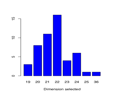
Figure 3: Bar charts of dimension selected $\widehat{m}$ over the 50 Monte Carlo replications for the projected estimator $\widehat{\boldsymbol{\beta}}_{\widehat{\boldsymbol{\lambda}},\widehat{m}}$.

Example 1	Example 2

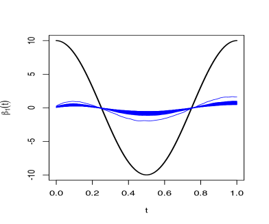
Figure 4: Plot of $\boldsymbol{\beta}_{1}^{*}$ (solid black line) and 50 Monte-Carlo replications of $\left[\widehat{\boldsymbol{\beta}}_{\widehat{\boldsymbol{\lambda}},\widehat{m}}\right]_{1}$ (blue lines).

6.4 Final estimator

Example 1	Example 2

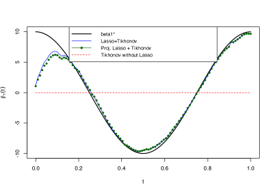
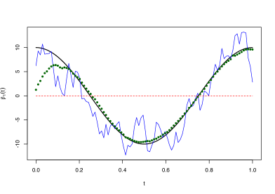
Figure 5: Plot of $\beta_{1}^{*}$ (solid black line), the solution of the Tikhonov regularization on the support of the Lasso estimator (dashed blue line) and on the whole support (dotted red line).

On Figure 5 we see that the Tikhonov regularization step reduces the bias in both examples. We can compare it with the effect of Tikhonov regularization step on the whole sample (i.e. without variable selection). It turns out that, in the case where all the covariates are kept, the algorithm (15) converges very slowly leading to poor estimates. The computation time of the estimators on an iMac 3,06 GHz Intel Core 2 Duo – with a non optimal code – are given in Table 3 for illustrative purposes.

	Lasso + Tikhonov	Proj. Lasso + Tikhonov	Tikhonov without Lasso
Example 1	7.5 min	9.3 min	36.0 min
Example 2	7.1 min	16.6 min	36.1 min

Table 3: Computation time of the estimators.

6.5 Application to the prediction of energy use of appliances

The aim is to study appliances energy consumption – which is the main source of energy consumption – in a low energy house situated in Stambruges (Belgium). The data are energy consumption measurements of electrical appliances (Appliances), light (light), temperature and humidity in the kitchen (T1 and RH1), in the living room (T2 and RH2), in the laundry room (T3 and RH3), in the office (T4 and RH4), in the bathroom (T5 and RH5), outside the building on the north side (T6 and RH6), in the ironing room (T7 and RH7), in the teenagers’ room (T8 and RH8) and in the parents’ room (T9 and RH9) as well as the temperature (T$\_$out), the pressure (Press$\_$mm$\_$hg), the humidity (RH$\_$out), wind speed (Windspeed), visibility (Visibility) and dewpoint temperature (Tdewpoint) from the weather station of Chievres, which is the weather station of the nearest airport.

Each variable is measured every 10 minutes from 11th january, 2016, 5pm to 27th may, 2016, 6pm.

The data is freely available on UCI Machine Learning Repository (archive.ics.uci.edu/ml/datasets/Appliances+energy+prediction) and has been studied by Candanedo et al. (2017). We refer to this article for a precise description of the experiment and a method to predict appliances energy consumption at a given time from the measurement of the other variables.

Here, we focus on the prediction of the mean appliances energy consumption of one day from the measure of each variable the day before (from midnight to midnight). We then dispose of a dataset of size $n=136$ with $p=24$ functional covariates. Our variable of interest is the logarithm of the mean appliances consumption. In order to obtain better results, we divide the covariates by their range. More precisely, the $j$-th curve of the $i$-th observation $X_{i}^{j}$ is transformed as follows

$$X_{i}^{j}(t)\leftarrow\frac{X_{i}^{j}(t)}{\max_{i^{\prime}=1,...,n;t^{\prime}}X_{i^{\prime}}^{j}(t^{\prime})-\min_{i^{\prime}=1,...,n;t^{\prime}}X_{i^{\prime}}^{j}(t^{\prime})}.$$

Recall that usual standardisation techniques are not possible for infinite-dimensional data since the covariance operator of each covariate is non invertible. The choice of the above transformation allows us to obtain covariates of the same order. All the variables are then centered.

We first plot the evolution of the norm of the coefficients as a function of $r$. The results are shown in Figure 6.

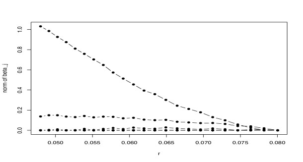
Figure 6: Plot of the norm of $\left[\widehat{\boldsymbol{\beta}}_{\widehat{\boldsymbol{\lambda}},\infty}\right]_{j}$, for $j=1,...,24$ as a function of $r$.

The variables selected by the Lasso criterion are the appliances energy consumption (Appliances), temperature of the laundry room (T3) and temperature of the teenage room (T8) curves. The corresponding slopes are represented in Figure 7. We observe that all the curves take larger values at the end of the day (after 8 pm). This indicates that the values of the three parameters that influence the most the mean appliances energy consumption of the day after are the one measured at the end of the day.

Appliances	T3	T8

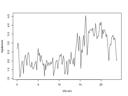
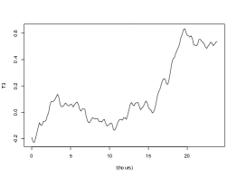
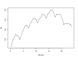
Figure 7: Plot of the coefficients $\left[\widehat{\boldsymbol{\beta}}_{\widehat{\boldsymbol{\lambda}},\infty}\right]_{j}$ for $j\in J(\widehat{\boldsymbol{\beta}}_{\widehat{\boldsymbol{\lambda}},\infty})=\{1,7,17\}$ corresponding to the coefficients associated to the appliance energy consumption curve (Appliances), temperature of the laundry room (T3) and temperature of the teenage room (T8).

Concluding remarks

The objective of the paper was to study how the theoretical results obtained for Lasso and Group-Lasso penalties can be adapted when the dimension of the covariates is infinite, which is, in particular, the case of functional data.

Discussion on the theoretical results and open-questions

As in finite dimension, the main issue is to control the relationship between the empirical norm naturally associated with the least squares criterion, related to the covariance matrix of the covariates, and the norm inducing the sparsity appearing in the penalty. The main problem here is that, as we prove in Lemma 1, these two norms cannot be equivalent in infinite dimension. The unprojected estimator seems to have very good performance in practice, and the solution can be computed easily. However, the rates of convergence of this estimator remains an open question. On the other hand, we prove sharp oracle inequalities for the projected estimator and we are able to define a data-based dimension selection criterion that achieves the best trade-off between the bias and the variance term. However, the rates of convergence of this estimator has not been proven to be optimal. Intuitively, it is not, and it seems likely that an adaptive Lasso procedure is needed to obtain an optimal rate in the minimax sense. These questions, which seem complex questions to solve, are left for future work.

We could also consider an alternative restricted eigenvalues assumption as it appears in Jiang et al. (2019) and suppose that there exist two positive numbers $\kappa_{1}$ and $\kappa_{2}$ such that

$$\|\boldsymbol{\beta}\|_{n}\geq\kappa_{1}\|\boldsymbol{\beta}\|-\kappa_{2}\|\boldsymbol{\beta}\|_{1},\text{ for all }\boldsymbol{\beta}\in\mathbf{H},$$

where we denote

$$\|\boldsymbol{\beta}\|_{1}:=\sum_{j=1}^{p}\|\beta_{j}\|_{j}\text{ for }\boldsymbol{\beta}=(\beta_{1},...,\beta_{p})\in\mathbf{H}.$$

This assumption does not suffer from the curse of dimensionality as the assumption $A_{RE(s)}$ does. However, contrary to the finite-dimensional case, the control of the probability that the assumption holds in the random design case is, to our knowledge, still an open question.

Discussion on the numerical results

From the simulation results, both methods seem to estimate the support of the slope coefficient $\boldsymbol{\beta}^{*}$ well. However, the projected method, which gives us the most accurate theoretical results, is quite difficult to implement in practice, due to the cost of constructing the spaces $\mathbf{H}^{(m)}$. On the contrary, the unprojected estimator seems to give interesting results, both in the simulation study and in the application on real data. However, the theoretical results (see for instance the remark after Corollary 1) argue for the choice of a finite value of $m$.

Discussion on the linearity assumption

The linearity assumption may be too restrictive in some contexts. A natural way to consider a nonlinear regression model is to assume that $Y=m(\mathbf{X})+\varepsilon$ where $m:\mathbf{H}\to\mathbb{R}$ is an unknown regression function. However, it has been shown by Mas (2012) that, without additional structural assumptions on $m$, this model suffers from the curse of dimensionality which manifests itself here by a very low minimax rate of convergence, typically logarithmic (see also the recent review by Ling and Vieu 2018 and the discussion in Geenens 2011; Chagny and Roche 2016). This is also the case for additive models

$$Y=m_{1}(X^{1})+\ldots+m_{p}(X^{p})+\varepsilon,$$

with $m_{j}$ unknown functions $m_{j}:\mathbb{H}_{j}\to\mathbb{R}$, which could be natural models to consider the sparsity problem.

This is the reason why semi-parametric models have been introduced and widely studied. In this category, we can mention for example the partially linear models (Kong et al., 2016; Wong et al., 2019),

$$Y=\langle\beta_{1},X^{1}\rangle_{1}+\ldots+\langle\beta_{p_{\infty}},X^{p_{\infty}}\rangle_{p_{\infty}}+m_{1}(X^{p_{\infty}+1})+\ldots+m_{p}(X^{p})+\varepsilon,$$

where we recall that $X^{p_{\infty}+1},\ldots,X^{p}$ are scalar or vector covariates and $X^{1},\ldots,X^{p_{\infty}}$ are functional covariates. The approach developed in this paper could be directly extended to this model by considering estimators by projection of $m_{j}$, as in Bunea et al. (2007). However, this introduces an additional bias that needs to be handled in the theoretical results and requires careful selection of the projection spaces and their dimensions.

This model has been generalized, for example, to the case of single-index models (see Novo et al. 2021 and references cited).

$$Y=g_{1}(\langle\beta_{1},X^{1}\rangle_{1})+\ldots+g_{p_{\infty}}(\langle\beta_{p_{\infty}},X^{p_{\infty}}\rangle_{p_{\infty}})+m_{1}(X^{p_{\infty}+1})+\ldots+m_{p}(X^{p})+\varepsilon,$$

where the $g_{j}$’s are unknown real functions. This type of model, poses theoretical questions more difficult to solve than the previous one, because the coefficients $\beta_{j}$ do not depend linearly on the observations.

Acknowledgements

I would like to thank Vincent Rivoirard and Gaëlle Chagny for their helpful advices and careful reading of the manuscript. The research is partly supported by the french Agence Nationale de la Recherche (ANR-18-CE40-0014 projet SMILES).

Appendix A Proofs

A.1 Proof of Lemma 1

Proof.

Let $J\subset\{1,\ldots,p\}$ such that $\dim(\mathbf{H}_{J})>{\rm rk}(\widehat{\boldsymbol{\Gamma}}_{J})$. This implies that $\dim(\rm{\ker}(\widehat{\boldsymbol{\Gamma}}_{J}))\geq 1$ and then that there exists $\boldsymbol{\delta}_{J}=(\delta_{j})_{j\in J}\in\mathbf{H}_{J}\backslash\{0\}$ such that $\widehat{\boldsymbol{\Gamma}}_{J}\boldsymbol{\delta}_{J}=0$. Define now from $\boldsymbol{\delta}_{J}$, $\boldsymbol{\delta}=(\delta_{1},\ldots,\delta_{p})\in\mathbf{H}$ such that $\delta_{j}=0$ if $j\notin J$.

Recall the definition of the operator

$$\widehat{\boldsymbol{\Gamma}}_{J}: \mathbf{H}_{J} \to\mathbf{H}_{J}$$

$$\boldsymbol{\beta}=(\beta_{j})_{j\in J} \mapsto\left(\frac{1}{n}\sum_{i=1}^{n}\sum_{j\in J}\langle\beta_{j},X_{i}^{j}\rangle_{j}X_{i}^{j^{\prime}}\right)_{j^{\prime}\in J},$$

and observe that

$$\|\boldsymbol{\delta}\|_{n}^{2}=\langle\widehat{\boldsymbol{\Gamma}}\boldsymbol{\delta},\boldsymbol{\delta}\rangle=0.$$

Moreover, $\boldsymbol{\delta}$ satisfies the constraints

$$0=\sum_{j\notin J}\lambda_{j}\|\delta_{j}\|_{j}\leq c_{0}\sum_{j\in J}\lambda_{j}\|\delta_{j}\|_{j},$$

for all choices of $\lambda_{1},\ldots,\lambda_{p}$ and for all $c_{0}>0$ which ends the proof. ∎

A.2 Proof of Proposition 1

Proof.

We prove only (8), Inequality (7) follows the same lines. The proof below is largely inspired by the proof of Lounici et al. (2011), using the improvement of Bellec and Tsybakov (2017) to obtain a sharp oracle inequality. First remark that some algebra gives us the following result, true for all $\boldsymbol{\beta}\in\mathbf{H}^{(m)}$,

$$\left\|\widehat{\boldsymbol{\beta}}_{\boldsymbol{\lambda},\infty}-\boldsymbol{\beta}^{*}\right\|_{n}^{2}-\left\|\boldsymbol{\beta}-\boldsymbol{\beta}^{*}\right\|_{n}^{2}=\frac{2}{n}\sum_{i=1}^{n}\langle\widehat{\boldsymbol{\beta}}_{\boldsymbol{\lambda},\infty}-\boldsymbol{\beta}^{*},\mathbf{X}_{i}\rangle\langle\widehat{\boldsymbol{\beta}}_{\boldsymbol{\lambda},\infty}-\boldsymbol{\beta},\mathbf{X}_{i}\rangle-\left\|\widehat{\boldsymbol{\beta}}_{\boldsymbol{\lambda},\infty}-\boldsymbol{\beta}\right\|_{n}^{2}$$ (16)

We can easily verify that the function

$$\gamma:\boldsymbol{\beta}\in\mathbf{H}\mapsto\frac{1}{n}\sum_{i=1}^{n}\left(Y_{i}-\langle\boldsymbol{\beta},\mathbf{X}_{i}\rangle\right)^{2}+2\sum_{j=1}^{p}\lambda_{j}\left\|\beta_{j}\right\|_{j}=\gamma_{1}(\boldsymbol{\beta})+\gamma_{2}(\boldsymbol{\beta})$$

is a proper convex function. Hence, $\widehat{\boldsymbol{\beta}}_{\boldsymbol{\lambda},\infty}$ is a minimum of $\gamma$ over $\mathbf{H}$ if and only if 0 is a subgradient $\partial\gamma(\widehat{\boldsymbol{\beta}}_{\boldsymbol{\lambda},\infty})$ of $\gamma$ at the point $\widehat{\boldsymbol{\beta}}_{\boldsymbol{\lambda},\infty}$.

The function $\gamma_{1}:\boldsymbol{\beta}\mapsto\frac{1}{n}\sum_{i=1}^{n}\left(Y_{i}-\langle\boldsymbol{\beta},\mathbf{X}_{i}\rangle\right)^{2}$ is differentiable on $\mathbf{H}$, with gradient,

$$\left(-\frac{2}{n}\sum_{i=1}^{n}(Y_{i}-\langle\boldsymbol{\beta},X_{i}\rangle)X_{i}^{j}\right)_{1\leq j\leq p}=-\frac{2}{n}\sum_{i=1}^{n}(Y_{i}-\langle\boldsymbol{\beta},X_{i}\rangle)\mathbf{X}_{i}$$

and $\gamma_{2}:\boldsymbol{\beta}\mapsto 2\sum_{j=1}^{p}\lambda_{j}\left\|\beta_{j}\right\|_{j}$ is differentiable on $D:=\{\boldsymbol{\beta}=(\boldsymbol{\beta}_{1},...,\boldsymbol{\beta}_{p})\in\mathbf{H},\ \forall j=1,...,p,\ \beta_{j}\neq 0\}$ with gradient

$$\left(2\lambda_{j}\frac{\beta_{j}}{\left\|\beta_{j}\right\|_{j}}\right)_{1\leq j\leq p}.$$

Since, for all $j=1,...,p$, the subdifferential of $\left\|\cdot\right\|_{j}$ at the point 0 is the closed unit ball of $\mathbf{H}_{j}$, the subdifferential of $\gamma_{2}:\boldsymbol{\beta}\mapsto 2\sum_{j=1}^{p}\lambda_{j}\left\|\beta_{j}\right\|_{j}$ at the point $\boldsymbol{\beta}\in D^{c}$, is the set

$$\partial\gamma_{2}(\boldsymbol{\beta})=\left\{\boldsymbol{\delta}=(\delta_{1},...,\delta_{p})\in\mathbf{H},\delta_{j}=2\lambda_{j}\frac{\beta_{j}}{\left\|\beta_{j}\right\|_{j}}\text{ if }\beta_{j}\neq 0,\left\|\delta_{j}\right\|_{j}\leq 2\lambda_{j}\text{ if }\beta_{j}=0\right\}.$$ (17)

Hence, the subdifferential of $\gamma$ at the point $\boldsymbol{\beta}=(\boldsymbol{\beta}_{1},...,\boldsymbol{\beta}_{p})\in\mathbf{H}$ is the set

$$\partial\gamma(\boldsymbol{\beta})=\left\{\boldsymbol{\theta}\in\mathbf{H},\ \exists\boldsymbol{\delta}\in\partial\gamma_{2}(\boldsymbol{\beta}),\ \boldsymbol{\theta}=-\frac{2}{n}\sum_{i=1}^{n}(Y_{i}-\langle\boldsymbol{\beta},\mathbf{X}_{i}\rangle)\mathbf{X}_{i}+\boldsymbol{\delta}\right\}.$$

Then, since $0\in\partial\gamma(\widehat{\boldsymbol{\beta}}_{\boldsymbol{\lambda},\infty})$, we know that there exists $\widehat{\boldsymbol{\delta}}=(\widehat{\delta}_{1},\ldots,\widehat{\delta}_{p})\in\partial\gamma_{2}(\widehat{\boldsymbol{\beta}}_{\boldsymbol{\lambda},\infty})$ such that

$$0=-\frac{2}{n}\sum_{i=1}^{n}(Y_{i}-\langle\widehat{\boldsymbol{\beta}}_{\boldsymbol{\lambda},\infty},\mathbf{X}_{i}\rangle)\mathbf{X}_{i}+\widehat{\boldsymbol{\delta}}=-\frac{2}{n}\sum_{i=1}^{n}(\langle\boldsymbol{\beta}^{*},\mathbf{X}_{i}\rangle+\varepsilon_{i}-\langle\widehat{\boldsymbol{\beta}}_{\boldsymbol{\lambda},\infty},\mathbf{X}_{i}\rangle)\mathbf{X}_{i}+\widehat{\boldsymbol{\delta}}.$$

Then

$$\frac{2}{n}\sum_{i=1}^{n}\langle\widehat{\boldsymbol{\beta}}_{\boldsymbol{\lambda},\infty}-\boldsymbol{\beta}^{*},\mathbf{X}_{i}\rangle\mathbf{X}_{i}=\frac{2}{n}\sum_{i=1}^{n}\varepsilon_{i}\mathbf{X}_{i}-\widehat{\boldsymbol{\delta}}$$

which implies

$$\frac{2}{n}\sum_{i=1}^{n}\langle\widehat{\boldsymbol{\beta}}_{\boldsymbol{\lambda},\infty}-\boldsymbol{\beta}^{*},\mathbf{X}_{i}\rangle\langle\widehat{\boldsymbol{\beta}}_{\boldsymbol{\lambda},\infty}-\boldsymbol{\beta},\mathbf{X}_{i}\rangle=\frac{2}{n}\sum_{i=1}^{n}\varepsilon_{i}\langle\widehat{\boldsymbol{\beta}}_{\boldsymbol{\lambda},\infty}-\boldsymbol{\beta},\mathbf{X}_{i}\rangle+\langle\boldsymbol{\beta}-\widehat{\boldsymbol{\beta}}_{\boldsymbol{\lambda},\infty},\widehat{\boldsymbol{\delta}}\rangle.$$ (18)

Now remark that, denoting $[\widehat{\beta}_{\boldsymbol{\lambda},\infty}]_{j}$ the $j$-th coordinate of $\widehat{\boldsymbol{\beta}}_{\boldsymbol{\lambda},\infty}$ we have, by definition of $\widehat{\boldsymbol{\delta}}$,

$$\begin{split}\langle\boldsymbol{\beta}-\widehat{\boldsymbol{\beta}}_{\boldsymbol{\lambda},\infty},\widehat{\boldsymbol{\delta}}\rangle&=\sum_{j=1}^{p}\langle\beta_{j}-[\widehat{\beta}_{\boldsymbol{\lambda},\infty}]_{j},\widehat{\delta}_{j}\rangle_{j}=\sum_{j=1}^{p}\langle\beta_{j},\widehat{\delta}_{j}\rangle_{j}-2\lambda_{j}\left\|[\widehat{\beta}_{\boldsymbol{\lambda},\infty}]_{j}\right\|_{j}\\ &\leq 2\sum_{j=1}^{p}\lambda_{j}\left(\left\|\beta_{j}\right\|_{j}-\left\|[\widehat{\beta}_{\boldsymbol{\lambda},\infty}]_{j}\right\|_{j}\right).\end{split}$$ (19)

Then inserting (18) and (19) in (16), we get

$$\left\|\widehat{\boldsymbol{\beta}}_{\boldsymbol{\lambda},\infty}-\boldsymbol{\beta}^{*}\right\|_{n}^{2}-\left\|\boldsymbol{\beta}-\boldsymbol{\beta}^{*}\right\|_{n}^{2} \leq \frac{2}{n}\sum_{i=1}^{n}\varepsilon_{i}\langle\boldsymbol{\beta}-\widehat{\boldsymbol{\beta}}_{\boldsymbol{\lambda},\infty},\mathbf{X}_{i}\rangle+2\sum_{j=1}^{p}\lambda_{j}\left(\left\|\beta_{j}\right\|_{j}-\left\|[\widehat{\beta}_{\boldsymbol{\lambda},\infty}]_{j}\right\|_{j}\right)$$ (20)

$$-\left\|\widehat{\boldsymbol{\beta}}_{\boldsymbol{\lambda},\infty}-\boldsymbol{\beta}\right\|_{n}^{2}.$$

Then the key result proven by Bellec et al. (2018, Lemma A.2) in a finite-dimensional context also holds in our infinite-dimensional context.

We now deal with the term involving the $\varepsilon_{i}$’s. Remark that, writing $\widehat{\boldsymbol{\beta}}_{\boldsymbol{\lambda},\infty}=\widehat{\boldsymbol{\beta}}_{\boldsymbol{\lambda},\infty}^{(m)}+\widehat{\boldsymbol{\beta}}_{\boldsymbol{\lambda},\infty}^{(\perp m)}$ where $\widehat{\boldsymbol{\beta}}^{(m)}_{\boldsymbol{\lambda},\infty}$ denotes the orthogonal projection of $\widehat{\boldsymbol{\beta}}_{\boldsymbol{\lambda},\infty}$ onto $\mathbf{H}^{(m)}$ and $\widehat{\boldsymbol{\beta}}^{(\perp m)}_{\boldsymbol{\lambda},\infty}$ denotes the orthogonal projection of $\widehat{\boldsymbol{\beta}}_{\boldsymbol{\lambda},\infty}$ onto $\left(\mathbf{H}^{(m)}\right)^{\perp}$,

$$\frac{1}{n}\sum_{i=1}^{n}\varepsilon_{i}\langle\boldsymbol{\beta}-\widehat{\boldsymbol{\beta}}_{\boldsymbol{\lambda},\infty},\mathbf{X}_{i}\rangle = \langle\boldsymbol{\beta}-\widehat{\boldsymbol{\beta}}_{\boldsymbol{\lambda},\infty},\frac{1}{n}\sum_{i=1}^{n}\varepsilon_{i}\mathbf{X}_{i}\rangle$$

$$= \langle\boldsymbol{\beta}-\widehat{\boldsymbol{\beta}}_{\boldsymbol{\lambda},\infty}^{(m)},\frac{1}{n}\sum_{i=1}^{n}\varepsilon_{i}\mathbf{X}_{i}\rangle+\langle\widehat{\boldsymbol{\beta}}_{\boldsymbol{\lambda},\infty}^{(\perp m)},-\frac{1}{n}\sum_{i=1}^{n}\varepsilon_{i}\mathbf{X}_{i}\rangle$$

$$\leq \sum_{j=1}^{p}\langle\beta_{j}-[\widehat{\boldsymbol{\beta}}_{\boldsymbol{\lambda},\infty}^{(m)}]_{j},\frac{1}{n}\sum_{i=1}^{n}\varepsilon_{i}X_{i}^{j}\rangle_{j}+\left\|\widehat{\boldsymbol{\beta}}_{\boldsymbol{\lambda},\infty}^{(\perp m)}\right\|\left\|\frac{1}{n}\sum_{i=1}^{n}\varepsilon_{i}\mathbf{X}_{i}\right\|$$

$$\leq \sum_{j=1}^{p}\left\|[\widehat{\beta}_{\boldsymbol{\lambda},\infty}^{(m)}]_{j}-\beta_{j}\right\|_{j}\left\|\frac{1}{n}\sum_{i=1}^{n}\varepsilon_{i}X_{i}^{j}\right\|_{j}+\left\|\widehat{\boldsymbol{\beta}}_{\boldsymbol{\lambda},\infty}^{(\perp m)}\right\|\left\|\frac{1}{n}\sum_{i=1}^{n}\varepsilon_{i}\mathbf{X}_{i}\right\|.$$

Let $\mathcal{A}=\bigcap_{j=1}^{p}\mathcal{A}_{j}$, with

$$\mathcal{A}_{j}=\left\{\left\|\frac{1}{n}\sum_{i=1}^{n}\varepsilon_{i}X_{i}^{j}\right\|_{j}\leq\lambda_{j}/2\right\}.$$

On the set $\mathcal{A}$,

$$\frac{2}{n}\sum_{i=1}^{n}\varepsilon_{i}\langle\boldsymbol{\beta}-\widehat{\boldsymbol{\beta}}_{\boldsymbol{\lambda},\infty},\mathbf{X}_{i}\rangle\leq\sum_{j=1}^{p}\lambda_{j}\left\|[\widehat{\beta}_{\boldsymbol{\lambda},\infty}^{(m)}]_{j}-\beta_{j}\right\|_{j}+\left\|\widehat{\boldsymbol{\beta}}_{\boldsymbol{\lambda},\infty}^{(\perp m)}\right\|\sqrt{\sum_{j=1}^{p}\lambda_{j}^{2}}.$$ (21)

Since the projector $\Pi_{m}$ verifies $C_{supp}$,

$$\left\|[\widehat{\beta}_{\boldsymbol{\lambda},\infty}^{(m)}]_{j}\right\|_{j}=\left\|\pi_{j}\Pi_{m}\widehat{\beta}_{\boldsymbol{\lambda},\infty}^{(m)}\right\|=\left\|\Pi_{m}\pi_{j}\widehat{\beta}_{\boldsymbol{\lambda},\infty}^{(m)}\right\|\leq\left\|\pi_{j}\widehat{\beta}_{\boldsymbol{\lambda},\infty}\right\|=\left\|[\widehat{\beta}_{\boldsymbol{\lambda},\infty}]_{j}\right\|_{j}$$

and gathering equations (20) and (21),

$$\begin{split}\left\|\widehat{\boldsymbol{\beta}}_{\boldsymbol{\lambda},\infty}-\boldsymbol{\beta}^{*}\right\|_{n}^{2}&-\left\|\boldsymbol{\beta}-\boldsymbol{\beta}^{*}\right\|_{n}^{2}+\sum_{j=1}^{p}\lambda_{j}\left\|[\widehat{\beta}_{\boldsymbol{\lambda},\infty}^{(m)}]_{j}-\beta_{j}\right\|_{j}\\ &\leq 2\sum_{j=1}^{p}\lambda_{j}\left(\left\|[\widehat{\beta}_{\boldsymbol{\lambda},\infty}^{(m)}]_{j}-\beta_{j}\right\|_{j}+\left\|\beta_{j}\right\|_{j}-\left\|[\widehat{\beta}_{\boldsymbol{\lambda},\infty}]_{j}\right\|_{j}\right)-\left\|\widehat{\boldsymbol{\beta}}_{\boldsymbol{\lambda},\infty}-\boldsymbol{\beta}\right\|_{n}^{2}+\left\|\widehat{\boldsymbol{\beta}}_{\boldsymbol{\lambda},\infty}^{(\perp m)}\right\|\sqrt{\sum_{j=1}^{p}\lambda_{j}^{2}}\\ &\leq 2\sum_{j=1}^{p}\lambda_{j}\left(\left\|[\widehat{\beta}_{\boldsymbol{\lambda},\infty}^{(m)}]_{j}-\beta_{j}\right\|_{j}+\left\|\beta_{j}\right\|_{j}-\left\|[\widehat{\beta}_{\boldsymbol{\lambda},\infty}^{(m)}]_{j}\right\|_{j}\right)-\left\|\widehat{\boldsymbol{\beta}}_{\boldsymbol{\lambda},\infty}-\boldsymbol{\beta}\right\|_{n}^{2}+\left\|\widehat{\boldsymbol{\beta}}_{\boldsymbol{\lambda},\infty}^{(\perp m)}\right\|\sqrt{\sum_{j=1}^{p}\lambda_{j}^{2}}\\ &\leq 4\!\sum_{j\in J(\boldsymbol{\beta})}\lambda_{j}\left\|[\widehat{\beta}_{\boldsymbol{\lambda},\infty}^{(m)}]_{j}-\beta_{j}\right\|_{j}-\left\|\widehat{\boldsymbol{\beta}}_{\boldsymbol{\lambda},\infty}-\boldsymbol{\beta}\right\|_{n}^{2}+\left\|\widehat{\boldsymbol{\beta}}_{\boldsymbol{\lambda},\infty}^{(\perp m)}\right\|\sqrt{\sum_{j=1}^{p}\lambda_{j}^{2}},\end{split}$$

since $\left\|\beta_{j}\right\|_{j}-\left\|[\widehat{\beta}_{\boldsymbol{\lambda},\infty}^{(m)}]_{j}\right\|_{j}\leq\left\|\beta_{j}-[\widehat{\beta}_{\boldsymbol{\lambda},\infty}^{(m)}]_{j}\right\|_{j}$. Finally

$$\begin{split}\left\|\widehat{\boldsymbol{\beta}}_{\boldsymbol{\lambda},\infty}-\boldsymbol{\beta}^{*}\right\|_{n}^{2}-\left\|\boldsymbol{\beta}-\boldsymbol{\beta}^{*}\right\|_{n}^{2}\leq&\ 3\!\sum_{j\in J(\boldsymbol{\beta})}\lambda_{j}\left\|[\widehat{\beta}_{\boldsymbol{\lambda},\infty}^{(m)}]_{j}-\beta_{j}\right\|_{j}-\!\sum_{j\notin J(\boldsymbol{\beta})}\lambda_{j}\left\|[\widehat{\beta}_{\boldsymbol{\lambda},\infty}^{(m)}]_{j}-\beta_{j}\right\|_{j}\\ &-\left\|\widehat{\boldsymbol{\beta}}_{\boldsymbol{\lambda},\infty}-\boldsymbol{\beta}\right\|_{n}^{2}+\left\|\widehat{\boldsymbol{\beta}}_{\boldsymbol{\lambda},\infty}^{(\perp m)}\right\|\sqrt{\sum_{j=1}^{p}\lambda_{j}^{2}}\end{split}$$ (22)

We consider now two cases :

1. $3\sum_{j\in J(\beta)}\lambda_{j}\left\|[\widehat{\beta}_{\boldsymbol{\lambda},\infty}^{(m)}]_{j}-\beta_{j}\right\|_{j}\geq\sum_{j\notin J(\beta)}\lambda_{j}\left\|[\widehat{\beta}_{\boldsymbol{\lambda},\infty}^{(m)}]_{j}-\beta_{j}\right\|_{j}$.

2. $3\sum_{j\in J(\beta)}\lambda_{j}\left\|[\widehat{\beta}_{\boldsymbol{\lambda},\infty}^{(m)}]_{j}-\beta_{j}\right\|_{j}<\sum_{j\notin J(\beta)}\lambda_{j}\left\|[\widehat{\beta}_{\boldsymbol{\lambda},\infty}^{(m)}]_{j}-\beta_{j}\right\|_{j}$.

First remark that in case 2., the result is obvious. Now, in case 1., we have, by definition of $\tilde{\kappa}_{n}^{(m)}(s)$,

$$\tilde{\kappa}_{n}^{(m)}(s)\leq\frac{\left\|\boldsymbol{\widehat{\beta}}_{\boldsymbol{\lambda},\infty}^{(m)}-\boldsymbol{\beta}\right\|_{n}}{\sqrt{\sum_{j\in J(\boldsymbol{\beta})}\left\|[\widehat{\beta}_{\boldsymbol{\lambda},\infty}^{(m)}]_{j}-\beta_{j}\right\|_{j}^{2}}}$$

or equivalently

$$\sqrt{\sum_{j\in J(\boldsymbol{\beta})}\left\|[\widehat{\beta}_{\boldsymbol{\lambda},\infty}^{(m)}]_{j}-\beta_{j}\right\|_{j}^{2}}\leq\frac{1}{\widetilde{\kappa}_{n}^{(m)}(s)}\left\|\widehat{\boldsymbol{\beta}}_{\boldsymbol{\lambda},\infty}^{(m)}-\boldsymbol{\beta}\right\|_{n}.$$

Then, using twice the fact that, for all $x,y\in\mathbb{R}$, $3xy\leq x^{2}+(9/4)y^{2}$, Equation (22) becomes,

$$\begin{split}\left\|\widehat{\boldsymbol{\beta}}_{\boldsymbol{\lambda},\infty}-\boldsymbol{\beta}^{*}\right\|_{n}^{2}&-\left\|\boldsymbol{\beta}-\boldsymbol{\beta}^{*}\right\|_{n}^{2}\\ &\leq 3\sqrt{\sum_{j\in J(\boldsymbol{\beta})}\lambda_{j}^{2}}\sqrt{\sum_{j\in J(\boldsymbol{\beta})}\left\|[\widehat{\beta}_{\boldsymbol{\lambda},\infty}^{(m)}]_{j}-\beta_{j}\right\|_{j}^{2}}-\left\|\widehat{\boldsymbol{\beta}}_{\boldsymbol{\lambda},\infty}-\boldsymbol{\beta}\right\|_{n}^{2}+\left\|\widehat{\boldsymbol{\beta}}_{\boldsymbol{\lambda},\infty}^{(\perp m)}\right\|\sqrt{\sum_{j=1}^{p}\lambda_{j}^{2}},\\ &\leq\frac{3}{\widetilde{\kappa}_{n}^{(m)}(s)}\sqrt{\sum_{j\in J(\boldsymbol{\beta})}\lambda_{j}^{2}}\left\|\widehat{\boldsymbol{\beta}}_{\boldsymbol{\lambda},\infty}^{(m)}-\boldsymbol{\beta}\right\|_{n}-\left\|\widehat{\boldsymbol{\beta}}_{\boldsymbol{\lambda},\infty}-\boldsymbol{\beta}\right\|_{n}^{2}+\left\|\widehat{\boldsymbol{\beta}}_{\boldsymbol{\lambda},\infty}^{(\perp m)}\right\|\sqrt{\sum_{j=1}^{p}\lambda_{j}^{2}},\\ &\leq\frac{3}{\widetilde{\kappa}_{n}^{(m)}(s)}\sqrt{\sum_{j\in J(\boldsymbol{\beta})}\lambda_{j}^{2}}\left(\left\|\widehat{\boldsymbol{\beta}}_{\boldsymbol{\lambda},\infty}-\boldsymbol{\beta}^{*}\right\|_{n}+\left\|\widehat{\boldsymbol{\beta}}_{\boldsymbol{\lambda},\infty}^{(\perp m)}\right\|_{n}\right)\\ &\qquad-\left\|\widehat{\boldsymbol{\beta}}_{\boldsymbol{\lambda},\infty}-\boldsymbol{\beta}\right\|_{n}^{2}+\left\|\widehat{\boldsymbol{\beta}}_{\boldsymbol{\lambda},\infty}^{(\perp m)}\right\|\sqrt{\sum_{j=1}^{p}\lambda_{j}^{2}}\\ &\leq\left\|\widehat{\boldsymbol{\beta}}_{\boldsymbol{\lambda},\infty}-\boldsymbol{\beta}^{*}\right\|_{n}^{2}+\frac{9}{4(\widetilde{\kappa}_{n}^{(m)}(s))^{2}}\sum_{j\in J(\boldsymbol{\beta})}\lambda_{j}^{2}-\left\|\widehat{\boldsymbol{\beta}}_{\boldsymbol{\lambda},\infty}-\boldsymbol{\beta}\right\|_{n}^{2}+R_{n,m}\\ \end{split},$$

where we recall that

$$R_{n,m}=\left(\left\|\widehat{\boldsymbol{\beta}}_{\boldsymbol{\lambda},\infty}^{(\perp m)}\right\|+\frac{3}{\widetilde{\kappa}_{n}^{(m)}(s)}\left\|\widehat{\boldsymbol{\beta}}_{\boldsymbol{\lambda},\infty}^{(\perp m)}\right\|_{n}\right)\sqrt{\sum_{j=1}^{p}\lambda_{j}^{2}},$$

which implies the expected result.

We turn now to the upper-bound on the probability of the complement of the event $\mathcal{A}$. Conditionally to $\mathbf{X}_{1},\ldots,\mathbf{X}_{n}$, since $\{\varepsilon_{i}\}_{1\leq i\leq n}\sim_{i.i.d}\mathcal{N}(0,\sigma^{2})$, the variable $\frac{1}{n}\sum_{i=1}^{n}\varepsilon_{i}X_{i}^{j}$ is a Gaussian random variable taking values in the Hilbert (hence Banach) space $\mathbb{H}_{j}$. Therefore, from Proposition 2, we know that, denoting $\mathbb{P}_{\mathbf{X}}(\cdot)=\mathbb{P}(\cdot|\mathbf{X}_{1},\ldots,\mathbf{X}_{n})$ and $\mathbb{E}_{\mathbf{X}}[\cdot]=\mathbb{E}[\cdot|\mathbf{X}_{1},\ldots,\mathbf{X}_{n}]$,

$$\mathbb{P}_{\mathbf{X}}(\mathcal{A}_{j}^{c})\leq 4\exp\left(-\frac{\lambda_{j}^{2}}{32\mathbb{E}_{\mathbf{X}}\left[\left\|\frac{1}{n}\sum_{i=1}^{n}\varepsilon_{i}X_{i}^{j}\right\|_{j}^{2}\right]}\right)=\exp\left(-\frac{nr_{n}^{2}}{32\sigma^{2}}\right),$$

since $\lambda_{j}^{2}=r_{n}^{2}\frac{1}{n}\sum_{i=1}^{n}\left\|X_{i}^{j}\right\|_{j}^{2}$ and

$$\mathbb{E}_{\mathbf{X}}\left[\left\|\frac{1}{n}\sum_{i=1}^{n}\varepsilon_{i}X_{i}^{j}\right\|_{j}^{2}\right]=\frac{1}{n^{2}}\sum_{i_{1},i_{2}=1}^{n}\mathbb{E}_{\mathbf{X}}\left[\varepsilon_{i_{1}}\varepsilon_{i_{2}}\langle X_{i_{1}}^{j},X_{i_{2}}^{2}\rangle_{j}\right]=\frac{\sigma^{2}}{n}\frac{1}{n}\sum_{i=1}^{n}\left\|X_{i}^{j}\right\|_{j}^{2}.$$

This implies that

$$\mathbb{P}(\mathcal{A}^{c})\leq p\exp\left(-\frac{nr_{n}^{2}}{32\sigma^{2}}\right)\leq p^{1-q},$$

as soon as $r_{n}\geq 4\sqrt{2}\sigma\sqrt{q\ln(p)/n}$.

∎

A.3 Proof of Theorem 1

Proof.

By definition of $\widehat{m}$, we know that, for all $m=1,\ldots,N_{n}$,

$$\frac{1}{n}\sum_{i=1}^{n}\left(Y_{i}-\langle\widehat{\boldsymbol{\beta}}_{\boldsymbol{\lambda},\widehat{m}},\mathbf{X}_{i}\rangle\right)^{2}+\kappa\sigma^{2}\frac{\widehat{m}}{n}\log(n)\leq\frac{1}{n}\sum_{i=1}^{n}\left(Y_{i}-\langle\widehat{\boldsymbol{\beta}}_{\boldsymbol{\lambda},m},\mathbf{X}_{i}\rangle\right)^{2}+\kappa\sigma^{2}\frac{m}{n}\log(n).$$

Now, we decompose the quantity, for all $\boldsymbol{\beta}\in\mathbf{H}$,

$$\frac{1}{n}\sum_{i=1}^{n}\left(Y_{i}-\langle\boldsymbol{\beta},\mathbf{X}_{i}\rangle\right)^{2} = \frac{1}{n}\sum_{i=1}^{n}\left(\langle\boldsymbol{\beta}^{*}-\boldsymbol{\beta},\mathbf{X}_{i}\rangle+\varepsilon_{i}\right)^{2}$$

$$= \left\|\boldsymbol{\beta}^{*}-\boldsymbol{\beta}\right\|_{n}^{2}+\frac{2}{n}\sum_{i=1}^{n}\varepsilon_{i}\langle\boldsymbol{\beta}^{*}-\boldsymbol{\beta},\mathbf{X}_{i}\rangle+\frac{1}{n}\sum_{i=1}^{n}\varepsilon_{i}^{2}.$$

and we obtain

$$\left\|\widehat{\boldsymbol{\beta}}_{\lambda,\widehat{m}}-\boldsymbol{\beta}^{*}\right\|_{n}^{2} \leq \left\|\widehat{\boldsymbol{\beta}}_{\lambda,m}-\boldsymbol{\beta}^{*}\right\|_{n}^{2}+\frac{2}{n}\sum_{i=1}^{n}\varepsilon_{i}\langle\widehat{\boldsymbol{\beta}}_{\boldsymbol{\lambda},\widehat{m}}-\widehat{\boldsymbol{\beta}}_{\lambda,m},\mathbf{X}_{i}\rangle$$ (23)

$$+\kappa\sigma^{2}\frac{m}{n}\log(n)-\kappa\sigma^{2}\frac{\widehat{m}}{n}\log(n).$$

Let $1/2>\eta>0$, since $2xy\leq\eta x^{2}+\eta^{-1}y^{2}$ for all $x,y\in\mathbb{R}$,

$$\frac{2}{n}\sum_{i=1}^{n}\varepsilon_{i}\langle\widehat{\boldsymbol{\beta}}_{\boldsymbol{\lambda},\widehat{m}}-\widehat{\boldsymbol{\beta}}_{\boldsymbol{\lambda},m},\mathbf{X}_{i}\rangle\leq\eta\left\|\widehat{\boldsymbol{\beta}}_{\boldsymbol{\lambda},\widehat{m}}-\widehat{\boldsymbol{\beta}}_{\boldsymbol{\lambda},m}\right\|_{n}^{2}+\eta^{-1}\nu_{n}^{2}\left(\frac{\widehat{\boldsymbol{\beta}}_{\boldsymbol{\lambda},\widehat{m}}-\widehat{\boldsymbol{\beta}}_{\boldsymbol{\lambda},m}}{\left\|\widehat{\boldsymbol{\beta}}_{\boldsymbol{\lambda},\widehat{m}}-\widehat{\boldsymbol{\beta}}_{\boldsymbol{\lambda},m}\right\|_{n}}\right),$$

where $\nu_{n}^{2}(\cdot):=\frac{1}{n}\sum_{i=1}^{n}\varepsilon_{i}\langle\cdot,X_{i}\rangle$. Now, we define the set :

$$\mathcal{B}_{m}:=\bigcap_{m^{\prime}=1}^{N_{n}}\left\{\sup_{f\in\mathbf{H}^{(\max\{m,m^{\prime}\})},\|f\|_{n}=1}\nu_{n}^{2}(f)<\frac{\kappa}{2\eta^{-1}}\log(n)\sigma^{2}\frac{\max\{m,m^{\prime}\}}{n}\right\}.$$ (24)

On the set $\mathcal{B}_{m}$, since $\widehat{\boldsymbol{\beta}}_{\boldsymbol{\lambda},\widehat{m}}-\widehat{\boldsymbol{\beta}}_{\boldsymbol{\lambda},m}\in\mathbf{H}^{(\max\{m,\widehat{m}\})}$,

$$\frac{2}{n}\sum_{i=1}^{n}\varepsilon_{i}\langle\widehat{\boldsymbol{\beta}}_{\boldsymbol{\lambda},\widehat{m}}-\widehat{\boldsymbol{\beta}}_{\boldsymbol{\lambda},m},\mathbf{X}_{i}\rangle \leq \eta\left\|\widehat{\boldsymbol{\beta}}_{\boldsymbol{\lambda},\widehat{m}}-\widehat{\boldsymbol{\beta}}_{\boldsymbol{\lambda},m}\right\|_{n}^{2}+\eta^{-1}\sup_{f\in\mathbf{H}^{(\max\{m,\widehat{m}\})},\|f\|_{n}^{2}=1}\nu_{n}^{2}(f)$$ (25)

$$\leq 2\eta\left\|\widehat{\boldsymbol{\beta}}_{\boldsymbol{\lambda},\widehat{m}}-\boldsymbol{\beta}^{*}\right\|_{n}^{2}+2\eta\left\|\widehat{\boldsymbol{\beta}}_{\boldsymbol{\lambda},m}-\boldsymbol{\beta}^{*}\right\|_{n}^{2}+\frac{\kappa}{2}\log(n)\sigma^{2}\frac{\max\{m,\widehat{m}\}}{n}.$$

Gathering equations (23) and (25), we get, on the set $\mathcal{A}\cap\mathcal{B}_{m}$,

$$(1-2\eta)\left\|\widehat{\boldsymbol{\beta}}_{\boldsymbol{\lambda},\widehat{m}}-\boldsymbol{\beta}^{*}\right\|_{n}^{2} \leq (1+2\eta)\left\|\widehat{\boldsymbol{\beta}}_{\boldsymbol{\lambda},m}-\boldsymbol{\beta}^{*}\right\|_{n}^{2}$$

$$+\frac{\kappa}{2}\log(n)\sigma^{2}\frac{\max\{m,\widehat{m}\}}{n}+\kappa\log(n)\sigma^{2}\frac{m}{n}-\kappa\log(n)\sigma^{2}\frac{\widehat{m}}{n}.$$

$$\leq (1+2\eta)\left\|\widehat{\boldsymbol{\beta}}_{\boldsymbol{\lambda},m}-\boldsymbol{\beta}^{*}\right\|_{n}^{2}+2\kappa\log(n)\sigma^{2}\frac{m}{n}.$$

and the quantity $\left\|\widehat{\boldsymbol{\beta}}_{\boldsymbol{\lambda},m}-\boldsymbol{\beta}^{*}\right\|_{n}^{2}$ is upper-bounded in Proposition 1. We obtain the expected result with $\tilde{\eta}=(1+2\eta)/(1-2\eta)-1>0$.

To conclude, since it has already been proven in Proposition 1 that $\mathbb{P}(\mathcal{A}^{c})\leq p^{1-q}$, it remains to prove that there exists a constant $C_{MS}>0$ such that

$$\mathbb{P}\left(\cup_{m=1}^{m}\mathcal{B}_{m}^{c}\right)\leq\frac{C_{MS}}{n}.$$

We have

$$\mathbb{P}\left(\cup_{m=1}^{m}\mathcal{B}_{m}^{c}\right)\leq\sum_{m=1}^{N_{n}}\sum_{m^{\prime}=1}^{N_{n}}\mathbb{P}\left(\sup_{f\in\mathbf{H}^{(\max\{m,m^{\prime}\})},\|f\|_{n}=1}\nu_{n}^{2}(f)\geq\frac{\kappa}{2\eta^{-1}}\log(n)\sigma^{2}\frac{\max\{m,m^{\prime}\}}{n}\right).$$

We apply Lemma 2 with $t=\left(\frac{\kappa}{2\eta^{-1}}\log(n)-1\right)\sigma^{2}\frac{\max\{m,m^{\prime}\}}{n}\leq\frac{\kappa}{6}\log(n)\sigma^{2}\frac{\max\{m,m^{\prime}\}}{n}$ and obtain

$$\mathbb{P}\left(\sup_{f\in\mathbf{H}^{(\max\{m,m^{\prime}\})},\|f\|_{n}=1}\nu_{n}^{2}(f)\geq\frac{\kappa}{6}\log(n)\sigma^{2}\frac{\max\{m,m^{\prime}\}}{n}\right)$$

$$\leq\exp\left(-2\kappa\log(n)\max\{m,m^{\prime}\}\min\left\{\frac{\kappa\log(n)}{6912},\frac{1}{1536}\right\}\right).$$

Suppose that $\kappa\log(n)>6912/1536=9/2$ (the other case could be treated similarly), we have, since $1\leq m\leq N_{n}\leq n$, and by bounding the second sum by an integral

$$\begin{split}\sum_{m=1}^{N_{n}}\sum_{m^{\prime}=1}^{N_{n}}\mathbb{P}\left(\sup_{f\in\mathbf{H}^{(\max\{m,m^{\prime}\})},\|f\|_{n}=1}\nu_{n}^{2}(f)\geq\frac{\kappa}{6}\log(n)\sigma^{2}\frac{\max\{m,m^{\prime}\}}{n}\right)&\\ &\leq\sum_{m=1}^{N_{n}}\left(\sum_{m^{\prime}=1}^{m}\exp\left(-\frac{\kappa\log(n)m}{768}\right)+\sum_{m^{\prime}=m+1}^{N_{n}}\exp\left(-\frac{\kappa\log(n)m^{\prime}}{768}\right)\right)\\ &\leq N_{n}\ n\exp\left(-\frac{\kappa\log(n)}{768}\right)+\frac{768N_{n}}{\kappa\log(n)}\exp\left(-\frac{\kappa\log(n)}{768}\right).\end{split}$$

Now choosing $\kappa>2304$ we know that there exists a universal constant $C_{MS}>0$ such that

$$\mathbb{P}\left(\cup_{m=1}^{N_{n}}\mathcal{B}_{m}^{c}\right)\leq C_{MS}/n.$$

Note that the minimal value 2304 for $\kappa$ is purely theoretical and does not correspond to a value of $\kappa$ which can reasonably be used in practice. ∎

A.4 Proof of Theorem 2

Proof.

In the proof, the notation $C,C^{\prime},C^{\prime\prime}>0$ denotes quantities which may vary from line to line but are always independent of $n$ or $m$.

Let $\mathcal{A}$ the set defined in the statement of Proposition 1 and $\mathcal{B}=\bigcap_{m=1}^{N_{n}}\mathcal{B}_{m}$ the set appearing in the proof of Theorem 1 (see Equation (24) p. 24). Following the proof of Theorem 1, we know that, on the set $\mathcal{A}\cap\mathcal{B}$, for all $m=1,\ldots,N_{n},M_{n}$, for all $\boldsymbol{\beta}\in\mathbf{H}^{(m)}$ such that $J(\boldsymbol{\beta})\leq s$, for all $\tilde{\eta}>0$,

$$\left\|\widehat{\boldsymbol{\beta}}_{\boldsymbol{\lambda},\widehat{m}}-\boldsymbol{\beta}^{*}\right\|_{n}^{2}\leq(1+\tilde{\eta})\|\boldsymbol{\beta}-\boldsymbol{\beta}^{*}\|_{n}^{2}+\frac{9}{4\left(\tilde{\kappa}_{n}^{(m)}(s)\right)^{2}}\sum_{j\in J(\boldsymbol{\beta})}\lambda_{j}^{2}+2\kappa\log(n)\sigma^{2}\frac{m}{n},$$ (26)

since $C(\tilde{\eta})\leq 2$. We also now that

$$\mathbb{P}(\mathcal{A}^{c})\leq p^{1-q}\text{ and }\mathbb{P}(\mathcal{B}^{c})\leq\frac{C_{MS}}{n}.$$

We define now the set $\mathcal{C}=\mathcal{C}_{1}\cap\mathcal{C}_{2}$ where

$$\mathcal{C}_{1} := \left\{\sup_{\boldsymbol{\beta}\in\mathbb{H}^{(N_{n})}\backslash\{0\}}\left|\frac{\|\boldsymbol{\beta}\|_{n}^{2}}{\|\boldsymbol{\beta}\|_{\boldsymbol{\Gamma}}^{2}}-1\right|\leq\frac{1}{2}\right\}$$

$$\mathcal{C}_{2} := \left\{\sup_{\boldsymbol{\beta}\in\mathbb{H}^{(N_{n})}\backslash\{0\}}\left|\frac{\|\boldsymbol{\beta}\|_{n}^{2}-\|\boldsymbol{\beta}\|_{\boldsymbol{\Gamma}}^{2}}{\|\boldsymbol{\beta}\|^{2}}\right|\leq\frac{1}{2}\right\}.$$

and prove that

$$\mathbb{P}(\mathcal{C}^{c})\leq 2n^{2}\exp(-c_{\max}n),\quad c_{\max}=\max\left\{(4b{\rm tr}(\boldsymbol{\Gamma})(4{\rm tr}(\boldsymbol{\Gamma})+1/2))^{-1};r_{\boldsymbol{\Gamma}}^{2}/16b\right\},$$ (27)

where $r_{\boldsymbol{\Gamma}}>0$ depends only on $\boldsymbol{\Gamma}$ and is defined below.

We apply Proposition 4 to bound

$$\mathbb{P}(\mathcal{C}_{1}^{c}) = \mathbb{P}\left(\sup_{\boldsymbol{\beta}\in\mathbb{H}^{(N_{n})}\backslash\{0\}}\left|\frac{\|\boldsymbol{\beta}\|_{n}^{2}-\|\boldsymbol{\beta}\|_{\boldsymbol{\Gamma}}^{2}}{\|\boldsymbol{\beta}\|_{\boldsymbol{\Gamma}}^{2}}\right|>\frac{1}{2}\right)$$ (28)

$$\leq 2N_{n}^{2}\exp\left(-\frac{n\rho^{2}(\boldsymbol{\Gamma}_{|N_{n}})}{4b\sum_{j=1}^{N_{n}}\tilde{v}_{j}\left(4\sum_{j=1}^{N_{n}}\tilde{v}_{j}+\frac{\rho(\boldsymbol{\Gamma}_{|N_{n}})}{2}\right)}\right)$$

$$\leq 2N_{n}^{2}\exp\left(-\frac{n\rho^{2}(\boldsymbol{\Gamma}_{|N_{n}})}{16b{\rm tr}^{2}(\boldsymbol{\Gamma}_{|N_{n}})}\right).$$

We remark that

$$\rho(\boldsymbol{\Gamma}_{|m})=\sup_{f\in\mathbb{H}^{(N_{n})}\backslash\{0\}}\frac{\|\boldsymbol{\Gamma}_{|N_{n}}f\|}{\|f\|}\underset{m\to+\infty}{\longrightarrow}\rho(\boldsymbol{\Gamma})\text{ and }{\rm tr}(\boldsymbol{\Gamma}_{|m})=\sum_{k=1}^{N_{n}}\langle\boldsymbol{\Gamma}\boldsymbol{\varphi}^{(k)},\boldsymbol{\varphi}^{(k)}\rangle\underset{m\to+\infty}{\longrightarrow}{\rm tr}(\boldsymbol{\Gamma}),$$

then

$$\frac{\rho(\boldsymbol{\Gamma}_{|m})}{{\rm tr}(\boldsymbol{\Gamma}_{|m})}\underset{m\to+\infty}{\longrightarrow}\frac{\rho(\boldsymbol{\Gamma})}{{\rm tr}(\boldsymbol{\Gamma})}>0,$$

and there exists a constant $r_{\boldsymbol{\Gamma}}>0$ such that, for all $m$,

$$\frac{\rho(\boldsymbol{\Gamma}_{|m})}{{\rm tr}(\boldsymbol{\Gamma}_{|m})}\geq r_{\boldsymbol{\Gamma}}.$$

Then from Equation (28), and the fact that $N_{n}\leq n$, we get that

$$\mathbb{P}(\mathcal{C}_{1}^{c})\leq 4n^{2}\exp\left(-\frac{r_{\boldsymbol{\Gamma}}n}{16b}\right).$$

We turn now to the upper-bound on the probability of $\mathcal{C}_{2}^{c}$ and apply again Proposition 4

$$\mathbb{P}\left(\sup_{\boldsymbol{\beta}\in\mathbb{H}^{(N_{n})}\backslash\{0\}}\left|\frac{\|\boldsymbol{\beta}\|_{n}^{2}-\|\boldsymbol{\beta}\|_{\boldsymbol{\Gamma}}^{2}}{\|\boldsymbol{\beta}\|^{2}}\right|>\frac{1}{2}\right) \leq 2N_{n}^{2}\exp\left(-\frac{n/4}{b\sum_{j=1}^{N_{n}}\tilde{v}_{j}\left(4\sum_{j=1}^{N_{n}}\tilde{v}_{j}+\frac{1}{2}\right)}\right)$$

$$\leq 2N_{n}^{2}\exp\left(-\frac{n}{4b{\rm tr}(\boldsymbol{\Gamma})\left(4{\rm tr}(\boldsymbol{\Gamma})+\frac{1}{2}\right)}\right)$$

and the upper-bound (27) comes from the fact that

$$\sum_{k=1}^{N_{n}}\tilde{v}_{k}=\sum_{k=1}^{N_{n}}\mathbb{E}[\langle\boldsymbol{\varphi}^{(k)},\mathbf{X}_{1}\rangle^{2}]=\sum_{k=1}^{N_{n}}\langle\boldsymbol{\Gamma}\boldsymbol{\varphi}^{(k)},\boldsymbol{\varphi}^{(k)}\rangle={\rm tr}(\boldsymbol{\Gamma}_{|N_{n}})\leq{\rm tr}(\boldsymbol{\Gamma}).$$

On the set $\mathcal{A}\cap\mathcal{B}\cap\mathcal{C}$, we have then, for all $m=1,\ldots,N_{n}$,

$$\left\|\widehat{\boldsymbol{\beta}}_{\boldsymbol{\lambda},\widehat{m}}-\boldsymbol{\beta}^{*}\right\|_{\boldsymbol{\Gamma}}^{2} \leq 2\left\|\widehat{\boldsymbol{\beta}}_{\boldsymbol{\lambda},\widehat{m}}-\boldsymbol{\beta}^{(*,m)}\right\|_{\boldsymbol{\Gamma}}^{2}+2\left\|\boldsymbol{\beta}^{(*,m)}-\boldsymbol{\beta}^{*}\right\|_{\boldsymbol{\Gamma}}^{2}$$

$$\leq 4\left\|\widehat{\boldsymbol{\beta}}_{\boldsymbol{\lambda},\widehat{m}}-\boldsymbol{\beta}^{(*,m)}\right\|_{n}^{2}+2\left\|\boldsymbol{\beta}^{(*,m)}-\boldsymbol{\beta}^{*}\right\|_{\boldsymbol{\Gamma}}^{2}$$

From (26), we get

$$\left\|\widehat{\boldsymbol{\beta}}_{\boldsymbol{\lambda},\widehat{m}}-\boldsymbol{\beta}^{*}\right\|_{\boldsymbol{\Gamma}}^{2} \leq C\left(\|\boldsymbol{\beta}-\boldsymbol{\beta}^{*}\|_{n}^{2}+\frac{1}{\left(\tilde{\kappa}_{n}^{(m)}(s)\right)^{2}}\sum_{j\in J(\boldsymbol{\beta})}\lambda_{j}^{2}+\kappa\frac{\log n}{n}\sigma^{2}m\right.$$

$$\quad\left.+\left\|\boldsymbol{\beta}^{*}-\boldsymbol{\beta}^{(*,m)}\right\|_{\boldsymbol{\Gamma}}^{2}\right),$$

for a constant $C>0$. Now remark that, on the set $\mathcal{C}_{1}$

$$\left\|\boldsymbol{\beta}^{(*,m)}-\boldsymbol{\beta}\right\|_{n}^{2}\leq\frac{3}{2}\left\|\boldsymbol{\beta}^{(*,m)}-\boldsymbol{\beta}\right\|_{\boldsymbol{\Gamma}}^{2}$$

and, for all $J\subset\{1,\ldots,p\}$, for all $\boldsymbol{\delta}\in\mathbf{H}^{(m)}$, such that $\sum_{j\in J}\|\delta_{j}\|_{j}^{2}\neq 0$,

$$\frac{1}{2}\frac{\|\boldsymbol{\delta}\|_{\boldsymbol{\Gamma}}^{2}}{\sqrt{\sum_{j\in J}\|\delta_{j}\|_{j}^{2}}}\leq\frac{\|\boldsymbol{\delta}\|_{n}^{2}}{\sqrt{\sum_{j\in J}\|\delta_{j}\|_{j}^{2}}}\leq\frac{3}{2}\frac{\|\boldsymbol{\delta}\|_{\boldsymbol{\Gamma}}^{2}}{\sqrt{\sum_{j\in J}\|\delta_{j}\|_{j}^{2}}},$$

which implies

$$\frac{1}{2}\kappa_{n}^{(m)}(s)\leq\tilde{\kappa}_{n}^{(m)}(s)\leq\frac{3}{2}\kappa_{n}^{(m)}(s).$$

We obtain

$$\left\|\widehat{\boldsymbol{\beta}}_{\boldsymbol{\lambda},\widehat{m}}-\boldsymbol{\beta}^{*}\right\|_{\Gamma}^{2} \leq C^{\prime}\min_{m=1,\ldots,N_{n}}\min_{\boldsymbol{\beta}\in\mathbf{H}^{(m)},|J(\boldsymbol{\beta})|\leq s}\left\{\|\boldsymbol{\beta}-\boldsymbol{\beta}^{*}\|_{\boldsymbol{\Gamma}}^{2}+\frac{1}{\left(\kappa_{n}^{(m)}(s)\right)^{2}}\sum_{j\in J(\boldsymbol{\beta})}\lambda_{j}^{2}\right.$$ (29)

$$\left.+\kappa\frac{\log n}{n}\sigma^{2}m+\left\|\boldsymbol{\beta}^{*}-\boldsymbol{\beta}^{(*,m)}\right\|_{\boldsymbol{\Gamma}}^{2}+\left\|\boldsymbol{\beta}^{*}-\boldsymbol{\beta}^{(*,m)}\right\|_{n}^{2}\right\}.$$

Now, let $\zeta_{n,m}=\frac{\log(n)}{\sqrt{n}}\|\boldsymbol{\beta}^{(*,\perp m)}\|$ and

$$\mathcal{D}:=\bigcap_{m=1}^{N_{n}}\left\{\|\boldsymbol{\beta}^{(*,\perp m)}\|_{n}^{2}\leq\|\boldsymbol{\beta}^{(*,\perp m)}\|_{\boldsymbol{\Gamma}}^{2}+\zeta_{n,m}\right\},$$

where we recall the notation $\boldsymbol{\beta}^{(*,\perp m)}=\boldsymbol{\beta}^{*}-\boldsymbol{\beta}^{(*,m)}$. We give now an upper-bound on $\mathbb{P}(\mathcal{D}^{c})$ which completes the proof. Remark that

$$\|\boldsymbol{\beta}^{(*,\perp m)}\|_{n}^{2}=\frac{1}{n}\sum_{i=1}^{n}\langle\boldsymbol{\beta}^{(*,\perp m)},\mathbf{X}_{i}\rangle^{2},$$

and that, for all $i=1,\ldots,n$,

$$\mathbb{E}\left[\langle\beta^{(*,\perp m)},\mathbf{X}_{i}\rangle^{2}\right]=\|\boldsymbol{\beta}^{(*,\perp m)}\|_{\boldsymbol{\Gamma}}^{2},$$

we can rewrite

$$\mathcal{D}:=\bigcap_{m=1}^{N_{n}}\left\{\frac{1}{n}\sum_{i=1}^{n}\left(\langle\boldsymbol{\beta}^{(*,\perp m)},\mathbf{X}_{i}\rangle^{2}-\mathbb{E}\left[\langle\boldsymbol{\beta}^{(*,\perp m)},\mathbf{X}_{1}\rangle^{2}\right]\right)\leq\zeta_{n,m}\right\}.$$

Hence

$$\mathbb{P}(\mathcal{D}^{c})\leq\sum_{m=1}^{N_{n}}\mathbb{P}\left(\frac{1}{n}\sum_{i=1}^{n}\left(\langle\boldsymbol{\beta}^{(*,\perp m)},\mathbf{X}_{i}\rangle^{2}-\mathbb{E}\left[\langle\boldsymbol{\beta}^{(*,\perp m)},\mathbf{X}_{1}\rangle^{2}\right]\right)>\zeta_{n,m}\right).$$

We upper-bound the quantities above using Bernstein’s inequality (Proposition 3, p. 3).

We have, for $\ell\geq 2$,

$$\mathbb{E}\left[\langle\boldsymbol{\beta}^{(*,\perp m)},\mathbf{X}_{i}\rangle^{2\ell}\rangle\right]\leq\|\boldsymbol{\beta}^{(*,\perp m)}\|^{2\ell}\mathbb{E}\left[\|\mathbf{X}_{i}\|^{2\ell}\right]\leq\frac{\ell!}{2}\|\boldsymbol{\beta}^{(*,\perp m)}\|^{2}v_{Mom}^{2}\left(\|\boldsymbol{\beta}^{(*,\perp m)}\|c_{Mom}\right)^{\ell-2},$$

applying Bernstein inequality, we get

$$\mathbb{P}(\mathcal{D}_{n}^{c})\leq\sum_{m=1}^{N_{n}}\exp\left(-\frac{n\zeta_{n,m}^{2}/2}{\|\boldsymbol{\beta}^{(*,\perp m)}\|^{2}v_{Mom}^{2}+\zeta_{n,m}\|\boldsymbol{\beta}^{(*,\perp m)}\|c_{Mom}}\right).$$

We get, since $N_{n}\leq n$,

$$\mathbb{P}(\mathcal{D}_{n}^{c})\leq N_{n}\exp\left(-\frac{\log^{2}(n)}{2v_{Mom}^{2}+\frac{\log(n)}{\sqrt{n}}c_{Mom}}\right)\leq\frac{C_{Mom}}{n},$$

with $C_{Mom}>0$ depending only on $v_{Mom}$ and $c_{Mom}$.

Then, on $\mathcal{A}\cap\mathcal{B}\cap\mathcal{C}\cap\mathcal{D}$, (29) becomes, for all $m=1,\ldots,N_{n}$,

$$\left\|\widehat{\boldsymbol{\beta}}_{\boldsymbol{\lambda},\widehat{m}}-\boldsymbol{\beta}^{*}\right\|_{\Gamma}^{2} \leq C\left(\|\boldsymbol{\beta}-\boldsymbol{\beta}^{*}\|_{\boldsymbol{\Gamma}}^{2}+\frac{1}{\left(\kappa_{n}^{(m)}(s)\right)^{2}}\sum_{j\in J(\boldsymbol{\beta})}\lambda_{j}^{2}+\kappa\frac{\log n}{n}\sigma^{2}m\right.$$

$$\quad\left.+\left\|\boldsymbol{\beta}^{(*,\perp m)}\right\|_{\boldsymbol{\Gamma}}^{2}+\zeta_{n,m}\right).$$

We then upper-bound $\zeta_{n,m}$ as follows

$$\zeta_{n,m}\leq\left(\kappa_{n}^{(m)}(s)\right)^{2}\left\|\boldsymbol{\beta}^{(*,\perp m)}\right\|^{2}+\frac{\log^{2}(n)}{n\left(\kappa_{n}^{(m)}(s)\right)^{2}}.$$

∎

Appendix B Control of empirical processes

Lemma 2.

For all $t>0$, for all $m$,

$$\mathbb{P}_{\mathbf{X}}\left(\sup_{\mathbf{f}\in\mathbf{H}^{(m)},\|f\|_{n}=1}\left(\frac{1}{n}\sum_{i=1}^{n}\varepsilon_{i}\langle\mathbf{f},\mathbf{X}_{i}\rangle\right)^{2}\geq\sigma^{2}\frac{m}{n}+t\right)$$

$$\leq\exp\left(-\min\left\{\frac{n^{2}t^{2}}{1536\sigma^{4}m};\frac{nt}{512\sigma^{2}}\right\}\right),$$

where $\mathbb{P}_{\mathbf{X}}(\cdot):=\mathbb{P}(\cdot|\mathbf{X}_{1},\ldots,\mathbf{X}_{n})$ is the conditional probability given $\mathbf{X}_{1},\ldots,\mathbf{X}_{n}$.

Proof of Lemma 2.

We follow the ideas of Baraud (2000). Let $m$ be fixed, and

$$S_{m}:=\left\{x=(x_{1},\ldots,x_{n})^{t}\in\mathbb{R}^{n},\exists\mathbf{f}\in\mathbb{H}^{(m)},\forall i,x_{i}=\langle\mathbf{f},\mathbf{X}_{i}\rangle\right\}.$$

We known that $S_{m}$ is a linear subspace of $\mathbb{R}^{n}$ and that

$$\sup_{\mathbf{f}\in\mathbf{H}^{(m)},\|f\|_{n}=1}\frac{1}{n}\sum_{i=1}^{n}\varepsilon_{i}\langle\mathbf{f},\mathbf{X}_{i}\rangle=\frac{1}{n}\sup_{x\in S_{m},x^{t}x=n}\varepsilon^{t}x=\frac{1}{\sqrt{n}}\sup_{x\in S_{m},x^{t}x=1}\varepsilon^{t}x=\frac{1}{\sqrt{n}}\sqrt{\varepsilon^{t}P_{m}\varepsilon},$$

where $\varepsilon=(\varepsilon_{1},\ldots,\varepsilon_{n})^{t}$ and $P_{m}$ is the matrix of the orthogonal projection onto $S_{m}$. This gives us

$$\mathbb{P}_{\mathbf{X}}\left(\sup_{\mathbf{f}\in\mathbf{H}^{(m)},\|f\|_{n}=1}\left(\frac{1}{n}\sum_{i=1}^{n}\varepsilon_{i}\langle\mathbf{f},\mathbf{X}_{i}\rangle\right)^{2}\geq\sigma^{2}\frac{m}{n}+t\right)=\mathbb{P}_{\mathbf{X}}\left(\varepsilon^{t}P_{m}\varepsilon\geq\sigma^{2}m+nt\right).$$

We apply now Bellec (2019, Theorem 3), with $A=P_{m}$ and obtain the expected results, since

$$\mathbb{E}[\varepsilon^{t}P_{m}\varepsilon]=\sigma^{2}\text{tr}(P_{m})=\sigma^{2}m,$$

and since the Frobenius norm $\|\cdot\|_{F}$ of $P_{m}$ is equal to $\|P_{m}\|_{F}=\sqrt{\text{tr}(\Pi_{m}^{t}\Pi_{m})}=\sqrt{m}$ and its matrix norm $\|P_{m}\|_{2}=1$. ∎

Appendix C Tails inequalities

Proposition 2.

Equivalence of tails of Banach-valued random variables (Ledoux and Talagrand, 1991, Equation (3.5) p. 59).

Let $X$ be a Gaussian random variable in a Banach space $(B,\|\cdot\|)$. For every $t>0$,

$$\mathbb{P}\left(\|X\|>t\right)\leq 4\exp\left(-\frac{t^{2}}{8\mathbb{E}\left[\|X\|^{2}\right]}\right).$$

Proposition 3.

Bernstein inequality (Birgé and Massart, 1998, Lemma 8).

Let $Z_{1},\ldots,Z_{n}$ be independent random variables satisfying the moments conditions

$$\frac{1}{n}\sum^{n}_{i=1}\mathbb{E}\left[\left|Z_{i}\right|^{\ell}\right]\leq\frac{\ell!}{2}v^{2}c^{\ell-2},\text{ for all }\ell\geq 2,$$

for some positive constants $v$ and $c$. Then, for any positive $\varepsilon$,

$$\mathbb{P}\left(\left|\frac{1}{n}\sum^{n}_{i=1}Z_{i}-\mathbb{E}\left[Z_{i}\right]\right|\geq\varepsilon\right)\leq 2\exp\left(-\frac{n\varepsilon^{2}/2}{v^{2}+c\varepsilon}\right).$$

Proposition 4.

Norm equivalence in finite subspaces.

Let $\mathbf{X}_{1},...,\mathbf{X}_{n}$ be i.i.d copies of a random variable $\mathbf{X}$ verifying Assumption $(H_{Mom}^{(1)})$.Then, for all $t>0$, for all weights $\mathbf{w}=(w_{1},...,w_{m})\in]0,+\infty[^{m}$,

$$\mathbb{P}\left(\sup_{\boldsymbol{\beta}\in\mathbf{H}^{(m)}\backslash\{0\}}\left|\frac{\|\boldsymbol{\beta}\|_{n}^{2}-\|\boldsymbol{\beta}\|_{\boldsymbol{\Gamma}}^{2}}{\|\boldsymbol{\beta}\|^{2}_{\mathbf{w}}}\right|>t\right)\leq 2m^{2}\exp\left(-\frac{nt^{2}}{b\sum_{j=1}^{m}\frac{\tilde{v}_{j}}{w_{j}}\left(4\sum_{j=1}^{m}\frac{\tilde{v}_{j}}{w_{j}}+t\right)}\right),$$ (30)

where $\|\boldsymbol{\beta}\|_{n}^{2}=\frac{1}{n}\sum_{i=1}^{n}\langle\boldsymbol{\beta},\mathbf{X}_{i}\rangle^{2}$, $\|\boldsymbol{\beta}\|_{\boldsymbol{\Gamma}}^{2}=\mathbb{E}\left[\|\boldsymbol{\beta}\|_{n}^{2}\right]$, and $\|\boldsymbol{\beta}\|_{\mathbf{w}}^{2}=\sum_{j=1}^{m}w_{j}\langle\boldsymbol{\beta},\boldsymbol{\varphi}^{(j)}\rangle^{2}$ and

$$\mathbb{P}\left(\sup_{\boldsymbol{\beta}\in\mathbf{H}^{(m)}\backslash\{0\}}\left|\frac{\|\boldsymbol{\beta}\|_{n}^{2}-\|\boldsymbol{\beta}\|_{\boldsymbol{\Gamma}}^{2}}{\|\boldsymbol{\beta}\|^{2}_{\boldsymbol{\Gamma}}}\right|>t\right)\leq 2m^{2}\exp\exp\left(-\frac{n\rho^{2}(\boldsymbol{\Gamma}_{|m})t^{2}}{b\sum_{j=1}^{m}\tilde{v}_{j}\left(4\sum_{j=1}^{m}\tilde{v}_{j}+t\rho(\boldsymbol{\Gamma}_{|m})\right)}\right).$$ (31)

Proof of Proposition 4.

We have, for all $\boldsymbol{\beta}\in\mathbf{H}^{(m)}$, $\|\boldsymbol{\beta}\|_{n}^{2}=\langle\widehat{\boldsymbol{\Gamma}}\boldsymbol{\beta},\boldsymbol{\beta}\rangle$. Hence,

$$\|\boldsymbol{\beta}\|_{n}^{2}-\|\boldsymbol{\beta}\|_{\boldsymbol{\Gamma}}^{2}=\langle(\widehat{\boldsymbol{\Gamma}}-\boldsymbol{\Gamma})\boldsymbol{\beta},\boldsymbol{\beta}\rangle=\sum_{j,k=1}^{m}\langle\boldsymbol{\beta},\boldsymbol{\varphi}^{(j)}\rangle\langle\boldsymbol{\beta},\boldsymbol{\varphi}^{(k)}\rangle\langle(\widehat{\boldsymbol{\Gamma}}-\boldsymbol{\Gamma})\boldsymbol{\varphi}^{(j)},\boldsymbol{\varphi}^{(k)}\rangle=b^{t}\Phi_{m}b,$$

with $b:=\left(\langle\boldsymbol{\beta},\boldsymbol{\varphi}^{(1)}\rangle,...,\langle\boldsymbol{\beta},\boldsymbol{\varphi}^{(m)}\rangle\right)^{t}$ and $\Phi_{m}=\left(\langle(\widehat{\boldsymbol{\Gamma}}-\boldsymbol{\Gamma})\boldsymbol{\varphi}^{(j)},\boldsymbol{\varphi}^{(k)}\rangle\right)_{1\leq j,k\leq m}$ which implies

$$\sup_{\boldsymbol{\beta}\in\mathbf{H}^{(m)}\backslash\{0\}}\left|\frac{\|\boldsymbol{\beta}\|_{n}^{2}-\|\boldsymbol{\beta}\|_{\boldsymbol{\Gamma}}^{2}}{\|\boldsymbol{\beta}\|_{\mathbf{w}}^{2}}\right| = \rho(W^{-1/2}\Phi_{m}W^{-1/2})\leq\sqrt{\text{tr}(W^{-1}\Phi_{m}\Phi_{m}^{t}W^{-1})}$$

$$= \sqrt{\sum_{j,k=1}^{m}\frac{\langle(\widehat{\boldsymbol{\Gamma}}-\boldsymbol{\Gamma})\boldsymbol{\varphi}^{(j)},\boldsymbol{\varphi}^{(k)}\rangle^{2}}{w_{j}w_{k}}},$$

where $\rho$ denotes the spectral radius, and $W$ the diagonal matrix with diagonal entries $(w_{1},\ldots,w_{m})$. We then have

$$\mathbb{P}\left(\sup_{\boldsymbol{\beta}\in\mathbf{H}^{(m)}\backslash\{0\}}\left|\frac{\|\boldsymbol{\beta}\|_{n}^{2}-\|\boldsymbol{\beta}\|_{\boldsymbol{\Gamma}}^{2}}{\|\boldsymbol{\beta}\|^{2}_{\mathbf{w}}}\right|>t\right) \leq \mathbb{P}\left(\sum_{j,k=1}^{m}\frac{\langle(\widehat{\boldsymbol{\Gamma}}-\boldsymbol{\Gamma})\boldsymbol{\varphi}_{j},\boldsymbol{\varphi}_{k}\rangle^{2}}{w_{j}w_{k}}>t^{2}\right)$$

$$\leq \mathbb{P}\left(\bigcup_{j,k=1}^{m}\left\{\frac{\langle(\widehat{\boldsymbol{\Gamma}}-\boldsymbol{\Gamma})\boldsymbol{\varphi}^{(j)},\boldsymbol{\varphi}^{(k)}\rangle^{2}}{w_{j}w_{k}}>p_{j,k}t^{2}\right\}\right),$$

$$\leq \sum_{j,k=1}^{m}\mathbb{P}\left(\frac{\left|\langle(\widehat{\boldsymbol{\Gamma}}-\boldsymbol{\Gamma})\boldsymbol{\varphi}^{(j)},\boldsymbol{\varphi}^{(k)}\rangle\right|}{\sqrt{w_{j}w_{k}}}>\sqrt{p_{j,k}}t\right),$$

where $p_{j,k}:=\frac{\tilde{v}_{j}\tilde{v}_{k}}{w_{j}w_{k}}\left(\sum_{\ell=1}^{m}\tilde{v}_{\ell}/w_{\ell}\right)^{-2}$ (remark that $\sum_{j,k=1}^{m}p_{j,k}=1$). Now, for all $j,k=1,...,m$,

$$\mathbb{P}\left(\frac{\left|\langle(\widehat{\boldsymbol{\Gamma}}-\boldsymbol{\Gamma})\boldsymbol{\varphi}^{(j)},\boldsymbol{\varphi}^{(k)}\rangle\right|}{\sqrt{w_{j}w_{k}}}>\sqrt{p_{j,k}}t\right)$$

$$=\mathbb{P}\left(\left|\frac{1}{n}\sum_{i=1}^{n}\frac{\langle\boldsymbol{\varphi}^{(j)},\mathbf{X}_{i}\rangle\langle\boldsymbol{\varphi}^{(k)},\mathbf{X}_{i}\rangle}{\sqrt{w_{j}w_{k}}}-\mathbb{E}\left[\frac{\langle\boldsymbol{\varphi}^{(j)},\mathbf{X}_{i}\rangle\langle\boldsymbol{\varphi}^{(k)},\mathbf{X}_{i}\rangle}{\sqrt{w_{j}w_{k}}}\right]\right|>\sqrt{p_{j,k}}t\right).$$

By Cauchy-Schwarz inequality, for all $\ell\geq 2$,

$$\mathbb{E}\left[\left|\frac{\langle\boldsymbol{\varphi}^{(j)},\mathbf{X}_{i}\rangle\langle\boldsymbol{\varphi}^{(k)},\mathbf{X}_{i}\rangle}{\sqrt{w_{j}w_{k}}}\right|^{\ell}\right] \leq \frac{\sqrt{\mathbb{E}\left[\langle\boldsymbol{\varphi}^{(j)},\mathbf{X}\rangle^{2\ell}\right]\mathbb{E}\left[\langle\boldsymbol{\varphi}^{(k)},\mathbf{X}\rangle^{2\ell}\right]}}{\sqrt{w_{j}w_{k}}^{\ell}}$$

$$\leq \ell!b^{\ell-1}\sqrt{\frac{\tilde{v}_{j}}{w_{j}}}^{\ell}\sqrt{\frac{\tilde{v}_{k}}{w_{k}}}^{\ell}=\frac{\ell!}{2}\;2b\frac{\tilde{v}_{j}}{w_{j}}\frac{\tilde{v}_{k}}{w_{k}}\;\left(b\sqrt{\frac{\tilde{v}_{j}}{w_{j}}}\sqrt{\frac{\tilde{v}_{k}}{w_{k}}}\right)^{\ell-2}.$$

Hence, Bernstein’s inequality (Lemma 3) implies that

$$\mathbb{P}\left(\frac{\left|\langle(\widehat{\boldsymbol{\Gamma}}-\boldsymbol{\Gamma})\boldsymbol{\varphi}^{(j)},\boldsymbol{\varphi}^{(k)}\rangle\right|}{\sqrt{w_{j}w_{k}}}>\sqrt{p_{j,k}}t\right)\leq 2\exp\left(-\frac{np_{j,k}t^{2}/2}{2b\frac{\tilde{v}_{j}\tilde{v}_{k}}{w_{j}w_{k}}+b\sqrt{\frac{\tilde{v}_{j}}{w_{j}}}\sqrt{\frac{\tilde{v}_{k}}{w_{k}}}\sqrt{p_{j,k}}t}\right),$$

and the definition of $p_{j,k}$ implies Equation (30).

We proceed similarly to prove Equation (31) from the upper-bound

$$\sup_{\boldsymbol{\beta}\in\mathbf{H}^{(m)}\backslash\{0\}}\left|\frac{\|\boldsymbol{\beta}\|_{n}^{2}-\|\boldsymbol{\beta}\|_{\boldsymbol{\Gamma}}^{2}}{\|\boldsymbol{\beta}\|_{\boldsymbol{\Gamma}}^{2}}\right|=\rho(\boldsymbol{\Gamma}_{|m}^{-1/2}\Phi_{m}\boldsymbol{\Gamma}_{|m}^{-1/2})\leq\rho(\Phi_{m})\rho(\boldsymbol{\Gamma}_{|m}^{-1})=\rho(\Phi_{m})\rho(\boldsymbol{\Gamma}_{|m})^{-1}$$

Following the same reasoning as above with $w_{1}=\ldots=w_{m}=1$, we get, for all $t>0$,

$$\mathbb{P}\left(\rho(\Phi_{m})>t\right)\leq 2m^{2}\exp\left(-\frac{nt^{2}}{b\sum_{j=1}^{m}\tilde{v}_{j}\left(4\sum_{j=1}^{m}\tilde{v}_{j}+t\right)}\right),$$

which proves Equation (31). ∎

References

- Aneiros and Vieu (2014) G. Aneiros and P. Vieu. Variable selection in infinite-dimensional problems. Statist. Probab. Lett., 94:12–20, 2014.
- Aneiros and Vieu (2016) G. Aneiros and P. Vieu. Sparse nonparametric model for regression with functional covariate. J. Nonparametr. Stat., 28(4):839–859, 2016.
- Aneiros-Pérez et al. (2004) G. Aneiros-Pérez, H. Cardot, G. Estévez-Pérez, and P. Vieu. Maximum ozone concentration forecasting by functional non-parametric approaches. Environmetrics, 15(7):675–685, 2004.
- Bach (2008) F. R. Bach. Consistency of the group lasso and multiple kernel learning. J. Mach. Learn. Res., 9:1179–1225, 2008.
- Baraud (2000) Y. Baraud. Model selection for regression on a fixed design. Probab. Theory Relat. Fields, 117(4):467–493, Aug 2000.
- Barron et al. (1999) A. Barron, L. Birgé, and P. Massart. Risk bounds for model selection via penalization. Probab. Theory Relat. Fields, 113(3):301–413, Feb 1999.
- Baudry et al. (2012) J.-P. Baudry, C. Maugis, and B. Michel. Slope heuristics: overview and implementation. Stat. Comput., 22(2):455–470, Mar 2012.
- Bellec and Tsybakov (2017) P. Bellec and A. Tsybakov. Bounds on the prediction error of penalized least squares estimators with convex penalty. In Modern problems of stochastic analysis and statistics, volume 208 of Springer Proc. Math. Stat., pages 315–333. Springer, Cham, 2017.
- Bellec (2019) P. C. Bellec. Concentration of quadratic forms under a bernstein moment assumption. 2019.
- Bellec et al. (2018) P. C. Bellec, G. Lecué, and A. B. Tsybakov. Slope meets Lasso: improved oracle bounds and optimality. Ann. Statist., 46(6B):3603–3642, 2018.
- Bertin et al. (2011) K. Bertin, E. Le Pennec, and V. Rivoirard. Adaptive Dantzig density estimation. Ann. Inst. Henri Poincaré Probab. Stat., 47(1):43–74, 2011.
- Bickel et al. (2009) P. J. Bickel, Y. Ritov, and A. B. Tsybakov. Simultaneous analysis of lasso and Dantzig selector. Ann. Statist., 37(4):1705–1732, 2009.
- Birgé and Massart (1998) L. Birgé and P. Massart. Minimum contrast estimators on sieves: exponential bounds and rates of convergence. Bernoulli, 4(3):329–375, 1998.
- Blazère et al. (2014) M. Blazère, J.-M. Loubes, and F. Gamboa. Oracle inequalities for a group lasso procedure applied to generalized linear models in high dimension. IEEE Trans. Inform. Theory, 60(4):2303–2318, 2014.
- Brunel et al. (2016) E. Brunel, A. Mas, and A. Roche. Non-asymptotic adaptive prediction in functional linear models. J. Multivariate Anal., 143:208–232, 2016.
- Bunea et al. (2007) F. Bunea, A. Tsybakov, and M. Wegkamp. Sparsity oracle inequalities for the Lasso. Electron. J. Stat., 1:169–194, 2007.
- Candanedo et al. (2017) L. M. Candanedo, V. Feldheim, and D. Deramaix. Data driven prediction models of energy use of appliances in a low-energy house. Energy and Buildings, 140, 2017.
- Cardot and Johannes (2010) H. Cardot and J. Johannes. Thresholding projection estimators in functional linear models. J. Multivariate Anal., 101(2):395–408, 2010.
- Cardot et al. (1999) H. Cardot, F. Ferraty, and P. Sarda. Functional linear model. Statist. Probab. Lett., 45(1):11–22, 1999.
- Cardot et al. (2003) H. Cardot, F. Ferraty, and P. Sarda. Spline estimators for the functional linear model. Statist. Sinica, 13(3):571–591, 2003.
- Cardot et al. (2007) H. Cardot, C. Crambes, and P. Sarda. Ozone pollution forecasting using conditional mean and conditional quantiles with functional covariates. In Statistical methods for biostatistics and related fields, pages 221–243. Springer, Berlin, 2007.
- Chagny and Roche (2016) G. Chagny and A. Roche. Adaptive estimation in the functional nonparametric regression model. J. Multivariate Anal., 146:105–118, 2016.
- Chan et al. (2014) N. H. Chan, C. Y. Yau, and R.-M. Zhang. Group LASSO for structural break time series. J. Amer. Statist. Assoc., 109(506):590–599, 2014.
- Chen et al. (1998) S. S. Chen, D. L. Donoho, and M. A. Saunders. Atomic decomposition by basis pursuit. SIAM Journal on Scientific Computing, 20(1):33–61, 1998.
- Chesneau and Hebiri (2008) C. Chesneau and M. Hebiri. Some theoretical results on the grouped variables Lasso. Math. Methods Statist., 17(4):317–326, 2008.
- Chiou et al. (2014) J.-M. Chiou, Y.-T. Chen, and Y.-F. Yang. Multivariate functional principal component analysis: a normalization approach. Statist. Sinica, 24(4):1571–1596, 2014.
- Chiou et al. (2016) J.-M. Chiou, Y.-F. Yang, and Y.-T. Chen. Multivariate functional linear regression and prediction. J. Multivariate Anal., 146:301–312, 2016.
- Comte and Johannes (2010) F. Comte and J. Johannes. Adaptive estimation in circular functional linear models. Math. Methods Statist., 19(1):42–63, 2010.
- Comte and Johannes (2012) F. Comte and J. Johannes. Adaptive functional linear regression. Ann. Statist., 40(6):2765–2797, 2012.
- Crambes et al. (2009) C. Crambes, A. Kneip, and P. Sarda. Smoothing splines estimators for functional linear regression. Ann. Statist., 37(1):35–72, 2009.
- Dalalyan et al. (2013) A. Dalalyan, M. Hebiri, K. Meziani, and J. Salmon. Learning heteroscedastic models by convex programming under group sparsity. In S. Dasgupta and D. McAllester, editors, Proceedings of the 30th International Conference on Machine Learning, volume 28 of Proceedings of Machine Learning Research, pages 379–387, Atlanta, Georgia, USA, 17–19 Jun 2013. PMLR. URL https://proceedings.mlr.press/v28/dalalyan13.html.
- Devijver (2017) E. Devijver. Model-based regression clustering for high-dimensional data: application to functional data. Adv. Data Anal. Classif., 11(2):243–279, 2017.
- Di et al. (2009) C.-Z. Di, C. M. Crainiceanu, B. S. Caffo, and N. M. Punjabi. Multilevel functional principal component analysis. Ann. Appl. Stat., 3(1):458–488, 2009.
- Fan et al. (2016) J. Fan, Y. Wu, M. Yuan, D. Page, J. Liu, I. M. Ong, P. Peissig, and E. Burnside. Structure-leveraged methods in breast cancer risk prediction. J. Mach. Learn. Res., 17:Paper No. 85, 15, 2016.
- Ferraty and Romain (2011) F. Ferraty and Y. Romain, editors. The Oxford handbook of functional data analysis. Oxford University Press, Oxford, 2011.
- Ferraty and Vieu (2000) F. Ferraty and P. Vieu. Dimension fractale et estimation de la régression dans des espaces vectoriels semi-normés. C. R. Acad. Sci. Paris Sér. I Math., 330(2):139–142, 2000.
- Ferraty and Vieu (2006) F. Ferraty and P. Vieu. Nonparametric functional data analysis. Springer Series in Statistics. Springer, New York, 2006. Theory and practice.
- Friedman et al. (2010) J. Friedman, T. Hastie, and R. Tibshirani. Regularization paths for generalized linear models via coordinate descent. Journal of Statistical Software, 33(1):1–22, 2010.
- Geenens (2011) G. Geenens. Curse of dimensionality and related issues in nonparametric functional regression. Stat. Surv., 5:30–43, 2011.
- Giraud (2015) C. Giraud. Introduction to high-dimensional statistics, volume 139 of Monographs on Statistics and Applied Probability. CRC Press, Boca Raton, FL, 2015.
- Goia and Vieu (2016) A. Goia and P. Vieu. An introduction to recent advances in high/infinite dimensional statistics [Editorial]. J. Multivariate Anal., 146:1–6, 2016.
- Grollemund et al. (2019) P.-M. Grollemund, C. Abraham, M. Baragatti, and P. Pudlo. Bayesian functional linear regression with sparse step functions. Bayesian Anal., 14(1):111–135, 2019.
- Huang and Zhang (2010) J. Huang and T. Zhang. The benefit of group sparsity. Ann. Statist., 38(4):1978–2004, 2010.
- Ivanoff et al. (2016) S. Ivanoff, F. Picard, and V. Rivoirard. Adaptive Lasso and group-Lasso for functional Poisson regression. J. Mach. Learn. Res., 17:Paper No. 55, 46, 2016.
- James et al. (2009) G. James, J. Wang, and J. Zhu. Functional linear regression that’s interpretable. Ann. Statist., 37(5A):2083–2108, 2009.
- Jiang et al. (2019) X. Jiang, P. Reynaud-Bouret, V. Rivoirard, L. Sansonnet, and R. M. Willett. A data-dependent weighted lasso under poisson noise. IEEE Trans. Inf. Theory, 65:1589–1613, 2019.
- Koltchinskii (2009) V. Koltchinskii. The dantzig selector and sparsity oracle inequalities. Bernoulli, 15(3):799–828, 08 2009.
- Koltchinskii and Minsker (2014) V. Koltchinskii and S. Minsker. -penalization in functional linear regression with subgaussian design. J. Éc. polytech. Math., 1:269–330, 2014.
- Kong et al. (2016) D. Kong, K. Xue, F. Yao, and H. H. Zhang. Partially functional linear regression in high dimensions. Biometrika, 103(1):147–159, 2016.
- Kwemou (2016) M. Kwemou. Non-asymptotic oracle inequalities for the Lasso and group Lasso in high dimensional logistic model. ESAIM Probab. Stat., 20:309–331, 2016.
- Laurini (2014) M. P. Laurini. Dynamic functional data analysis with non-parametric state space models. J. Appl. Stat., 41(1):142–163, 2014.
- Ledoux and Talagrand (1991) M. Ledoux and M. Talagrand. Probability in Banach spaces, volume 23 of Ergebnisse der Mathematik und ihrer Grenzgebiete (3) [Results in Mathematics and Related Areas (3)]. Springer-Verlag, Berlin, 1991. Isoperimetry and processes.
- Li et al. (2016) D. Li, J. Qian, and L. Su. Panel data models with interactive fixed effects and multiple structural breaks. J. Amer. Statist. Assoc., 111(516):1804–1819, 2016.
- Li and Hsing (2007) Y. Li and T. Hsing. On rates of convergence in functional linear regression. J. Multivariate Anal., 98(9):1782–1804, 2007.
- Lin and Zhang (2006) Y. Lin and H. H. Zhang. Component selection and smoothing in multivariate nonparametric regression. Ann. Statist., 34(5):2272–2297, 2006.
- Ling and Vieu (2018) N. Ling and P. Vieu. Nonparametric modelling for functional data: selected survey and tracks for future. Statistics, 52(4):934–949, 2018.
- Liu and Yu (2013) H. Liu and B. Yu. Asymptotic properties of Lasso+mLS and Lasso+Ridge in sparse high-dimensional linear regression. Electron. J. Stat., 7:3124–3169, 2013.
- Lounici et al. (2011) K. Lounici, M. Pontil, S. van de Geer, and A. B. Tsybakov. Oracle inequalities and optimal inference under group sparsity. Ann. Statist., 39(4):2164–2204, 2011.
- Mas (2012) A. Mas. Lower bound in regression for functional data by representation of small ball probabilities. Electron. J. Statist., 6:1745–1778, 2012.
- Mas and Ruymgaart (2015) A. Mas and F. Ruymgaart. High-dimensional principal projections. Complex Anal. Oper. Theory, 9(1):35–63, 2015.
- Meier et al. (2008) L. Meier, S. van de Geer, and P. Bühlmann. The group Lasso for logistic regression. J. R. Stat. Soc. Ser. B Stat. Methodol., 70(1):53–71, 2008.
- Nardi and Rinaldo (2008) Y. Nardi and A. Rinaldo. On the asymptotic properties of the group lasso estimator for linear models. Electron. J. Stat., 2:605–633, 2008.
- Novo et al. (2021) S. Novo, G. Aneiros, and P. Vieu. Sparse semiparametric regression when predictors are mixture of functional and high-dimensional variables. TEST, 30(2):481–504, 2021.
- Pham et al. (2010) H. Pham, S. Mottelet, O. Schoefs, A. Pauss, V. Rocher, C. Paffoni, F. Meunier, S. Rechdaoui, and S. Azimi. Estimation simultanée et en ligne de nitrates et nitrites par identification spectrale UV en traitement des eaux usées. L’eau, l’industrie, les nuisances, 335:61–69, 2010.
- Preda and Saporta (2005) C. Preda and G. Saporta. PLS regression on a stochastic process. Comput. Statist. Data Anal., 48(1):149–158, 2005.
- Ramsay and Dalzell (1991) J. O. Ramsay and C. J. Dalzell. Some tools for functional data analysis. J. Roy. Statist. Soc. Ser. B, 53(3):539–572, 1991. With discussion and a reply by the authors.
- Ramsay and Silverman (2005) J. O. Ramsay and B. W. Silverman. Functional data analysis. Springer Series in Statistics. Springer, New York, second edition, 2005.
- Roche (2018) A. Roche. Local optimization of black-box function with high or infinite-dimensional inputs. Comp. Stat., 33(1):467–485, 2018.
- Sangalli (2018) L. Sangalli. The role of statistics in the era of big data. Statist. Probab. Lett., 136:1–3, 2018.
- Shin (2009) H. Shin. Partial functional linear regression. J. Statist. Plann. Inference, 139(10):3405 – 3418, 2009.
- Shin and Lee (2012) H. Shin and M. H. Lee. On prediction rate in partial functional linear regression. J. Multivariate Anal., 103(1):93 – 106, 2012.
- Sørensen et al. (2012) H. Sørensen, A. Tolver, M. H. Thomsen, and P. H. Andersen. Quantification of symmetry for functional data with application to equine lameness classification. J. Appl. Statist., 39(2):337–360, 2012.
- Tibshirani (1996) R. Tibshirani. Regression shrinkage and selection via the lasso. J. Roy. Statist. Soc. Ser. B, 58(1):267–288, 1996.
- Tsybakov (2009) A. B. Tsybakov. Introduction to nonparametric estimation. Springer Series in Statistics. Springer, New York, 2009.
- van de Geer (2014) S. van de Geer. Weakly decomposable regularization penalties and structured sparsity. Scand. J. Stat., 41(1):72–86, 2014.
- van de Geer and Bühlmann (2009) S. A. van de Geer and P. Bühlmann. On the conditions used to prove oracle results for the Lasso. Electron. J. Stat., 3:1360–1392, 2009.
- Wang and Leng (2007) H. Wang and C. Leng. Unified LASSO estimation by least squares approximation. J. Amer. Statist. Assoc., 102(479):1039–1048, 2007.
- Wang et al. (2007) H. Wang, R. Li, and C.-L. Tsai. Tuning parameter selectors for the smoothly clipped absolute deviation method. Biometrika, 94(3):553–568, 2007.
- Wang et al. (2021) W. Wang, Y. Sun, and J. Wang. Latent group detection in functional partially linear regression models. Biometrics, Sept. 2021.
- Wold (1975) H. Wold. Soft modelling by latent variables: the non-linear iterative partial least squares (NIPALS) approach. In Perspectives in probability and statistics (papers in honour of M. S. Bartlett on the occasion of his 65th birthday), pages 117–142. Applied Probability Trust, Univ. Sheffield, Sheffield, 1975.
- Wong et al. (2019) R. K. W. Wong, Y. Li, and Z. Zhu. Partially linear functional additive models for multivariate functional data. Journal of the American Statistical Association, 114(525):406–418, 2019.
- Xu et al. (2020) W. Xu, H. Ding, R. Zhang, and H. Liang. Estimation and inference in partially functional linear regression with multiple functional covariates. Journal of Statistical Planning and Inference, 209:44–61, 2020.
- Yang and Zou (2015) Y. Yang and H. Zou. A fast unified algorithm for solving group-lasso penalize learning problems. Stat. Comput., 25(6):1129–1141, 2015.
- Yuan and Lin (2006) M. Yuan and Y. Lin. Model selection and estimation in regression with grouped variables. J. R. Stat. Soc. Ser. B Stat. Methodol., 68(1):49–67, 2006.
- Zhao et al. (2016) Y. Zhao, M. Chung, B. A. Johnson, C. S. Moreno, and Q. Long. Hierarchical feature selection incorporating known and novel biological information: identifying genomic features related to prostate cancer recurrence. J. Amer. Statist. Assoc., 111(516):1427–1439, 2016.