Formation of nonlinear X-waves in condensed matter systems

Abstract

X-waves are an example of a localized wave packet solution of the homogeneous wave equation, and can potentially arise in any area of physics relating to wave phenomena, such as acoustics, electromagnetism, or quantum mechanics. They have been predicted in condensed matter systems such as atomic Bose-Einstein condensates in optical lattices, and were recently observed in exciton-polariton condensates. Here we show that polariton X-waves result from an interference between two separating wave packets that arise from the combination of a locally hyperbolic dispersion relation and nonlinear interactions. We show that similar X-wave structures could also be observed in expanding spin-orbit coupled Bose-Einstein condensates.

I Introduction

X-waves are a well-known example of a localized wave packet, and have been central to many efforts to generate optical pulses that are able to resist diffraction Hernández-Figueroa et al. (2007). They were originally introduced as a superposition of Bessel beams. that are non-diffracting solutions of the homogeneous wave equation Lu and Greenleaf (1992a)

$$[\bm{\nabla}^{2}-(1/c^{2})\partial^{2}_{t}]\Psi(\mathbf{r},t)=0,$$ (1)

and can thus be encountered in a wide range of fields such as acoustics, electromagnetism, quantum physics and potentially seismology or gravitation.

Solitons and solitary waves are another famous type of non-spreading wave packet which rely on a balance between dispersion and nonlinear self-focussing to remain localized during propagation Eiermann et al. (2004); Amo et al. (2009); Sich et al. (2012). However, X-waves do not require any nonlinearity in the wave equation, a feature which they share with Bessel beams and other remarkable solutions, such as Airy beams—non-spreading solutions of the Schrödinger equation discovered by Berry and Balazs Berry and Balazs (1979) which have peculiar self-accelerating and self-healing properties.

X-waves, Bessel and Airy beams are non-physical solutions since, like plane waves, they cannot be normalized and hence would require an infinite energy to maintain their spectacular properties through propagation. These solutions were thus initially considered a mathematical curiosity, but it was later realized and experimentally demonstrated that square-integrable approximations retain their surprising features for a significant amount of time Durnin et al. (1987); Lu and Greenleaf (1992b). For Airy beams, such demonstration even came several decades later its original prediction Siviloglou et al. (2007); Voloch-Bloch et al. (2013). A later experiment confirmed Airy beams’ self-healing property, showing their ability to self-reconstruct even after strong perturbations, and also demonstrated their robustness in adverse environments, such as in scattering and turbulent media Broky et al. (2008). Similarly, approximations of X-wave packets must also reproduce their characteristic features, including X-shape preserving propagation, but only for a finite time.

While Airy beams are typically produced by pulse shaping and can be made arbitrarily close to their ideal (unphysical) blueprint, it has been found that X-waves can conveniently be spontaneously generated in dispersive and interacting media that feature a hyperbolic dispersion, i.e., where the effective mass takes opposite signs in transverse dimensions. In this instance they are called “nonlinear X-waves” or X-wave solitons Conti et al. (2003); Trapani et al. (2003). We will adopt this X-wave terminology to refer to any similar phenomenology that results from the combined effects of hyperbolic dispersion and interactions. We note that this is at best a finite-time approximation of an idealised scenario which, as we shall discuss, opens new doors for alternative interpretations in a realistic implementation.

X-waves were first discussed in a condensed matter context with a theoretical proposal for their observation in an atomic Bose-Einstein condensate (BEC) Conti and Trillo (2004), where the hyperbolic dispersion can be engineered by placing the BEC in a 1D optical lattice, “bending” the dispersion near the edge of the Brillouin zone. Similar band engineering was proposed by Sedov et al. with Bragg exciton-polaritons Sedov et al. (2015), using a periodical arrangement of quantum wells to realize hyperbolic metamaterials that support X-wave solutions.

However, a suitably hyperbolic dispersion naturally occurs with exciton-polaritons, which are bosonic quasiparticles that arise from the strong coupling between photons and excitons in semiconductors microcavities Kavokin et al. (2017). As a result of their hybrid nature, they possess a highly non-parabolic and tunable dispersion relation that provides inflection points, and thus regions of negative effective mass, without the need for externally imposed potentials or Bragg polaritons. In 2D, one can find hyperbolic regions that sustain X-waves solutions, as was first pointed out by Voronych et al. Voronych et al. (2016), who also studied these solutions extensively. Another feature of polaritons is that their interaction strength is tunable to some extent, either by changing the excitonic (interacting) fraction or by altering the density of particles, which allows the study of X-waves in both the weakly and strongly interacting regimes. Recently, the experimental observation of polaritonic X-waves was reported Gianfrate et al. (2018). In this experiment polariton interactions were used to reshape an initial Gaussian packet (easily created with a laser pulse) into an X-wave by imparting it with a finite momentum above the inflection point of the dispersion. While this yielded a beautiful proof of principle of the underlying idea, important questions remain open. In particular, although one cannot hope to create an ideal X-wave, how close can one can get through this interaction-based mechanism? In a realistic polariton system, how robust is the nonlinear instability that converts a Gaussian wave packet into an X-wave Voronych et al. (2016)? And for how long can an X-wave generated in this manner display its expected characteristics?

To answer these questions, we examine the nonlinear X-wave formation mechanism under the prism of the wavelet transform (WT), a spectral decomposition that provides unique insights into the nontrivial dynamics of wave packet propagation. Previously this technique has been used to explain and fully characterize so-called self-interfering packets (SIPs), another phenomenology observed with polaritons due to an inflection point in the dispersion relation. This results in negative-mass effects (counter propagation) coexisting with normal (forward) propagation, producing a constant flow of propagating fringes Colas and Laussy (2016). While purely a linear wave phenomenon, the SIP can also be triggered due by a nonlinearity leading to the spread of the wave packet across the inflection point in momentum space. The formation of a SIP, powered by nonlinear interactions, was recently observed in an atomic spin-orbit coupled BEC Khamehchi et al. (2017); Colas et al. (2018).

In this paper, we show how the wavelet transform provides a new understanding of the nature and formation of a nonlinear X-wave. The X-wave is indeed found to be a transient effect that occurs during the reshaping of a Gaussian wave packet under the combined effects of a non-parabolic dispersion and repulsive interactions. The spatial interference of two resulting sub-packets travelling at different speeds accounts for the X-wave pattern. The polaritonic X-wave can thus be understood as another type of SIP rather than a shape-preserving non-interacting “soliton”. This confirms the self-interference mechanism is the key to understanding the general problem of wave packet propagation under nontrivial dispersion relations that feature inflection points and thus both negative and infinite effective masses, either with or without nonlinearity.

This paper is organized as follows. In Sec. II we introduce our method of analysis, and provide an idealized example of X-wave formation in a complex wave equation with a purely hyperbolic dispersion relation and a weak nonlinearity. In Sec. III we demonstrate how the same phenomenon arises in the formation of X-waves in an exciton-polariton system. Section IV proposes how X-waves can be formed in atomic Bose-Einstein condensates with artificial spin-orbit coupling, instead of an additional optical lattice potential Conti et al. (2003). We conclude in Sec. V.

II Hyperbolic dispersion

We start with the simplest system allowing the generation of nonlinear X-waves, a Gross-Pitaevskii equation for the field $\psi(x,y)$

$$i\hbar\partial_{t}\psi(x,y)=H_{\mathrm{hyp}}\psi(x,y).$$ (2)

The nonlinear operator

$$H_{\mathrm{hyp}}=\frac{\hbar^{2}k_{x}^{2}}{2m_{x}}+\frac{\hbar^{2}k_{y}^{2}}{2m_{y}}+g|\psi(x,y)|^{2}\,,$$ (3)

has masses of opposite signs in the $x$ and $y$ dimensions $m_{x}=-m_{y}$, and thus the system combines a hyperbolic dispersion with repulsive interactions. A 3D representation of the hyperbolic dispersion is shown in Fig. 1(a). The dispersion is parabolic in both directions but with an inverted curvature in the $x$ direction, as seen in Fig. 1(b). The last term in Eq. (3) accounts for the nonlinear interaction, characterised by the constant $g$. An example of a nonlinear X-wave formation out of an initial Gaussian wave packet imparted with a momentum $k_{x}^{0}$ is shown in Fig. 1(c–f) foo (a). One can see the typical X-shape appearing in the density as it propagates. Phase singularities with opposite winding also appear when the X-wave fully forms, here marked as blue and red dots. However the X-wave does not maintain its shape and breaks in larger packets at long time, Fig. 1(f), much like square integrable Airy beam approximations lose their self-accelerating property during propagation Siviloglou et al. (2007).

The X-wave formation mechanism can be better understood when considering the field $\psi(\bm{r},t)$ in a different representation space. Various spectral representations of the wave function are accessible through the Fourier Transform, such as the space-energy $\psi(\bm{r},E)$ or the momentum-energy $\psi(\bm{k},E)$ (also called far-field) representations. They can provide useful information on, e.g., relaxation processes yielding the Bose-Einstein condensation Estrecho et al. (2018), or the characterization of topological effects with the presence of Dirac cones or flat-bands Jacqmin et al. (2014); Baboux et al. (2016).
However, such representations are poorly adapted for the detection of a transient interference effect, as either the spatial or the temporal dynamics vanishes when integrating towards the momentum or energy domains. An alternative method of analysis is to make use of the Wavelet Transform (WT) — a convenient manner in which to simultaneously represent the field in both position and momentum space at a given instant in time.

The WT was initially introduced in signal processing to obtain a representation of the signal in both time and frequency. It has proven to be particularly useful to analyse the interference between different wave packets Baker et al. (2012) or more recently the self-interference from a single wave packet Colas and Laussy (2016); Colas et al. (2018). Unlike the usual Fourier Transform that is based on the decomposition of the signal into a sum of unphysical states (delocalized sine and cosine functions), the WT uses more physical states with localized wavelets $\mathcal{G}$ as basis functions.

For a 1D wave packet $\psi(x)$, the general WT reads Debnath and Shah (2015):

$$\mathbb{W}(x,k)=(1/\sqrt{|k|})\int_{-\infty}^{+\infty}\psi(x^{\prime})\mathcal{G}^{\ast}[(x^{\prime}-x)/k]\mathrm{d}x^{\prime}\,.$$ (4)

A suitable representation when analysing Schrödinger wave packets is the Gabor wavelet:

$$\mathcal{G}(x)=\sqrt[4]{\pi}\exp(iw_{\mathcal{G}}x)\exp(-x^{2}/2)\,,$$ (5)

This wavelet family consists of a Gaussian envelope, which is an elementary constituent of the Schrödinger dynamics, with an internal phase that oscillates at a defined wavelet-frequency $\omega_{\mathcal{G}}$. The physical momentum $k$ can be retrieved from the WT parameters (wavelet-frequency, grid specifics etc) using a numerical procedure that is detailed in Ref. Colas et al. (2018). The quantity $|\mathbb{W}(x,k)|^{2}$ thus measures the cross-correlation between the wavelet $\mathcal{G}(x)$ and the wave function $\psi(x)$. This allows us to show in a transparent way the position $x$ in real-space of the different $k$-components of the wave packet.

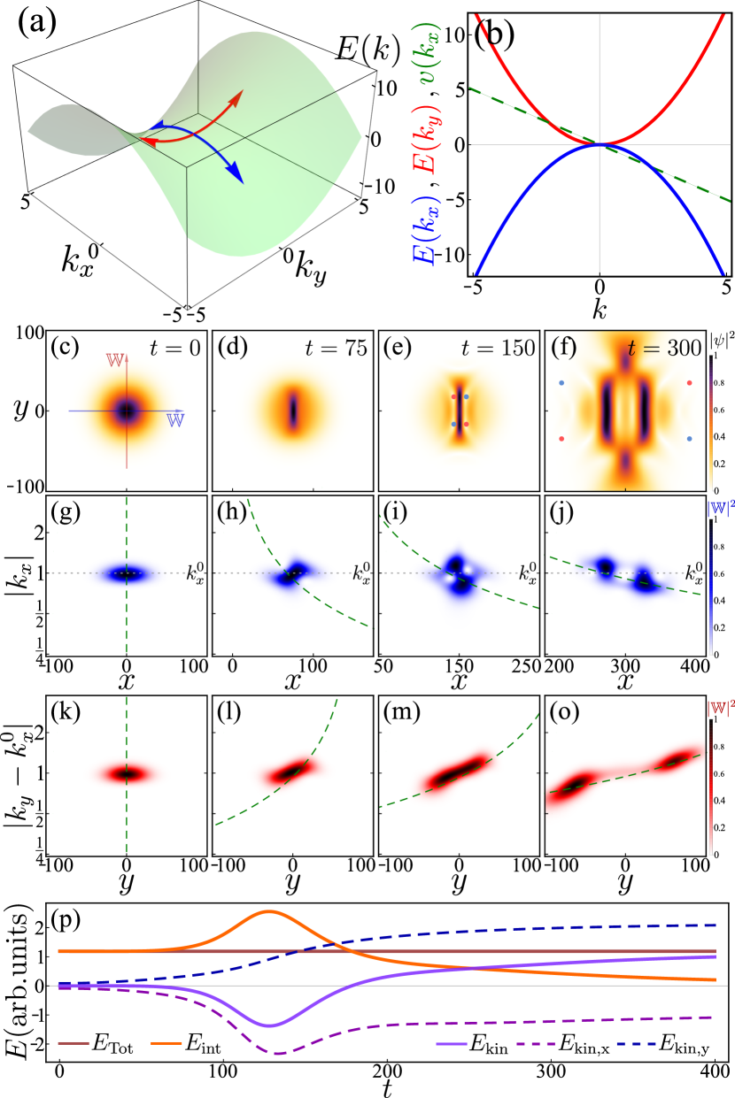
Figure 1: X-wave formation and propagation for a hyperbolic dispersion. (a) 2D hyperbolic-dispersion. (b) Effective dispersion along $k_{x}$ and $k_{y}$, with $v(k_{x})$. (c–f) Evolution of the density $|\psi(x,y)|^{2}$ at selected times, starting from a Gaussian wave packet with $\sigma=20$ and imparted with a momentum $k_{x}^{0}=1$. Light-blue (red) dots indicate a $\pm 2\pi$ phase winding. (g–j) Corresponding wavelet energy density $|\mathbb{W}|^{2}$ computed along the $x$ direction. (k–o) Idem but computed along the $y$ direction. The green dashed curve shows the displacement of the $k_{x,y}$-components $d(k_{x,y})=v(k_{x,y})t$. (p) Evolution of the components of the energy: Total (brown), interaction (orange), kinetic (purple) with its two components along $x$ (dashed-dark purple) and $y$ (dashed-dark blue). Parameters: $\hbar=m_{x}=-1$, $g=0.003$. Supplemental Movie 1 provides an animation of the nonlinear X-wave formation for this system foo (b).

We apply the 1D-WT to the slice $\psi(x,y=0)$, i.e., along the direction of propagation, and at different times of the X-wave evolution, as shown in Fig. 1(g–j). The mechanism leading to the X-wave formation appears clearly in this spectral representation. At $t=0$, the wavelet energy density is tightly distributed around the value $k_{x}^{0}$, Fig. 1(c,g), which is the momentum initially imparted to the wave packet. Since the wave packet is not spatially confined by any external potential, the initial interaction energy is converted into kinetic energy, leading to an increase of the packet’s spread in momentum space, as previously observed in 1D systems Colas et al. (2018). This first distortion can be seen in the WT, Fig. 1(h), along with its consequence on the packet shape in real space, which shrinks in the $x$ direction, Fig. 1(d). Indeed, in the direction of propagation, the group velocity $v(k_{x})=\partial_{k_{x}}E(k_{x},0)$ decreases as the momentum increases, see the dashed-green curve for $v(k_{x})$ in Fig 1(b). This means that a particle acquiring additional momentum will travel more slowly. This feature is the key ingredient for the X-wave formation. As the packet’s spread in $k_{x}$ keeps increasing, the latter effect leads to the break up of the initial packet into two sub-packets, located at different $k_{x}$ and hence travelling at different velocities. In Fig. 1(g–j), the green dashed line shows the expected displacement of the $k_{x}$-components $d(k_{x})=v(k_{x})t$. In real space, the sub-packet with the lowest momentum but with the highest group velocity formed at the tail overtakes the other sub-packet formed at a higher momentum but propagating at a lower velocity. The spatial overlap of these two sub-packets creates the interference fringes that are at the heart of the peculiar X-shape of the wave packet.

We also apply the 1D-WT to the transverse direction of the center of the packet while following its drift in $x$, i.e., we consider the $y$-WT of $\psi(x=v(k_{x}^{0})t,y)$. The wavelet energy density $|\mathbb{W}(y,k_{y}-k_{x}^{0})|^{2}$ foo (c) is shown in Fig. 1(k–o). The interactions also lead to an increase of the packet’s spread in $k_{y}$, followed by a breaking of the packet into two distinct parts, but unlike for the $x$-direction, this time the sub-packet with a higher momentum travels faster than the one with a lower momentum, which prevents any interference from occurring.

To complete the X-wave analysis, we take a closer look at the energy exchanges occurring during the wave packet propagation. The Gaussian wave packet set as an initial condition undergoes reshaping under the joint action of the dispersion and repulsive interaction, under the constraint of conservation of the total energy:

$$E_{\mathrm{Tot}}=E_{\mathrm{kin}}+E_{\mathrm{int}}\\ =\int\big{[}E(\mathbf{k})-E(\mathbf{k}_{0})\big{]}|\psi(\mathbf{k})|^{2}\,d\mathbf{k}+\int\frac{g}{2}|\psi(\mathbf{r})|^{4}\,d\mathbf{r}\,.$$ (6)

The kinetic energy $E_{\mathrm{kin}}$ is here computed in momentum space in order to remove the important energy shift $E(\mathbf{k}_{0})$ induced by the imparted momentum set in the initial condition. The interaction energy $E_{\mathrm{int}}$ is more conveniently computed in real space. The evolution of these different energy components is shown in Fig. 1(p), with the total, interaction and kinetic energies plotted in brown, orange and purple, respectively. It is also instructive to consider the components of the kinetic energy $E_{\mathrm{kin},x}$ and $E_{\mathrm{kin},y}$ along the $x$ and $y$ directions. They are plotted as dark purple and blue dashed lines, respectively. Note that at $t=0$, $E_{\mathrm{kin}}=0$ as $E_{\mathrm{kin},x}=-E_{\mathrm{kin},y}$ since the initial packet is a symmetrical Gaussian that spreads equally in both $x$ and $y$ directions of the hyperbolic dispersion with $E(k_{x})=-E(k_{y})$, which cancels the overall kinetic energy. For the same reason, an increasing spread in momentum along the $k_{y}$ direction leads to an increase of $E_{\mathrm{kin},y}$ whereas an increasing spread in momentum along the $k_{x}$ direction actually leads to a decrease of $E_{\mathrm{kin},x}$. As the total energy has to be conserved, this causes a momentary rise of the interaction energy as observed in Fig. 1(p). The energy peak corresponds to the time of maximum interference between the sub-packets, and also corresponds to the time of the emergence of the phase singularities. At long times, when the new packets spread out, all the interaction energy is converted into kinetic energy, leaving the system behaving essentially as linear waves. The above discussion illustrates neatly how the WT analysis captures the key physics that rules the wave packet reshaping, namely, the interplay between the hyperbolic dispersion and its resulting negative energy, and the interactions which peak to break the packet and create phase singularities.

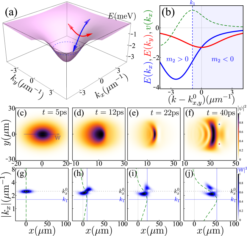
Figure 2: Exciton-polariton X-wave dynamics. (a) 2D lower polariton dispersion. The dashed-blue line indicates the position of the inflection points. (b) Effective dispersion in two transverse directions from the point $(k_{x}=$2.5\text{\,}\mu\reciprocal\mathrm{m}$,k_{y}=$0\text{\,}\mu\reciprocal\mathrm{m}$)$, with $v(k_{x})$. (c–f) Evolution of the polariton density $|\psi|^{2}$ at selected times. Light-blue (red) dots indicate a $\pm 2\pi$ phase winding. (g–j) Corresponding wavelet energy density $|\mathbb{W}|^{2}$ computed along the $x$ direction. The packet is imparted with a momentum $k_{x}^{0}=$2.5\text{\,}\mu\reciprocal\mathrm{m}$$, above the inflection point $k_{1}$. The green dashed curve shows the displacement of the $k_{x}$-components $d(k_{x})=v(k_{x})t$. The vertical blue line correspond to displacement $d(k_{1})$ delimiting the interference area. Supplemental Movie 2 provides an animation of the nonlinear X-wave formation for this system foo (b).

III Exciton-polaritons

We now study a realistic and physical exciton-polariton system, whose dynamics can be well-captured by the following two-component Gross-Pitaevkii operator Carusotto and Ciuti (2004); Gianfrate et al. (2018):

$$H_{\mathrm{pol}}=\begin{pmatrix}\frac{\hbar\bm{k}^{2}}{2m_{\mathrm{C}}}+\Delta-i\frac{\gamma_{\mathrm{C}}}{2}&\frac{\Omega_{\mathrm{R}}}{2}\\ \frac{\Omega_{\mathrm{R}}}{2}&\frac{\hbar\bm{k}^{2}}{2m_{\mathrm{X}}}-i\frac{\gamma_{\mathrm{X}}}{2}+g_{\mathrm{X}}|\psi_{\mathrm{X}}|^{2}\end{pmatrix}\,,$$ (7)

which acts on the spinor field $\bm{\psi}=(\psi_{\mathrm{C}},\psi_{\mathrm{X}})^{T}$. The parameter $m_{\mathrm{C},(\mathrm{X})}$ is the photon (exciton) mass, $\Delta$ the detuning between the photonic and excitonic modes and $\Omega_{\mathrm{R}}$ their coupling strength. Both fields have an independent decay rate $\gamma_{\mathrm{C,(X)}}$. The nonlinearity is here introduced through the exciton-exciton interaction with a strength $g_{\mathrm{X}}$. Diagonalising the non-interacting and dissipationless part of the operator leads to dressed upper and lower polariton modes:

$$E_{\mathrm{U,L}}=\frac{\hbar\bm{k}^{2}}{2m_{+}}+\frac{\Delta}{2}\pm\sqrt{\left(\frac{\hbar\bm{k}^{2}}{2m_{-}}-\frac{\Delta}{2}\right)^{2}+\left(\frac{\Omega_{\mathrm{R}}}{2}\right)^{2}}\,,\\$$ (8)

where $m_{\pm}=(m_{\mathrm{C}}\pm m_{\mathrm{X}})/2m_{\mathrm{C}}m_{\mathrm{X}}$. In the following, we use a similar set of parameters to Gianfrante et al. Gianfrate et al. (2018). The lower branch $E_{\mathrm{L}}$ is plotted in Fig. 2(a) and shows a circularly symmetric profile, approximately parabolic at small $\bm{|k|}$, and possessing an inflection point at $k_{1}=$1.61\text{\,}\mu\reciprocal\mathrm{m}$$ (dashed-blue line). An X-wave can be generated by exciting the branch above the inflection point in any given direction, where the effective dispersion thus appears locally hyperbolic, as shown in Fig. 2(b). The dynamical evolution of a polariton wave packet can be obtained by solving the following equation:

$$i\hbar\partial_{t}\bm{\psi}=H_{\mathrm{pol}}\bm{\psi}+\mathbf{P}\,,$$ (9)

where $\mathbf{P}=(\mathrm{LG}_{00}\mathrm{e}^{-(t-t_{0})^{2}/2\sigma_{t}}\mathrm{e}^{-i\omega_{\mathrm{L}}t}\mathrm{e}^{-ik_{x}^{0}x},0)^{\mathrm{T}}$ stands for the pulse excitation. The photonic field is excited with a Gaussian pulse arriving at time $t_{0}$, with a temporal spread $\sigma_{t}$, an energy $\omega_{\mathrm{L}}$ and with an imparted momentum $k_{x}^{0}$. The pulse parameters are chosen so that only the lower branch is populated ($\omega_{\mathrm{L}}=$-3\text{\,}\mathrm{meV}$$, $\sigma_{t}=$0.5\text{\,}\mathrm{ps}$$), preventing Rabi oscillations between the two modes Dominici et al. (2014). The initial momentum of the pulse is set to be above the inflection point of the branch, at $k_{x}^{0}=$2.5\text{\,}\mu\reciprocal\mathrm{m}$$. Selected time frames of the density evolution are presented in Fig. 2(c–f). Approximately $10\text{\,}\mathrm{ps}$ after the pulse arrival, the wave packet starts to distort, Fig. 2(d), then shrinks, Fig. 2(e), before forming a typical X-shape profile Fig. 2(f) along with phase singularities. The formation of a vortex-antivortex pair is here again a consequence of the hyperbolic topology of the dispersion relation, which leads to an inwards polaritons flow along the propagation direction and outwards in the transverse one, as noted in Ref. Gianfrate et al. (2018).

The WT analysis reveals that the exact same formation mechanism as for the ideal hyperbolic dispersion occurs in the polariton system. Shortly after the pulse arrival, the wavelet energy density is distributed around $k_{x}^{0}$, Fig. 2(g). The packet then spreads in $k_{x}$ due to the interaction, Fig. 2(h), and narrows in the $x$-dimension in real space, Fig. 2(d). Above the inflection point $k_{1}$, $v(k_{x})=\partial_{k_{x}}E(k_{x},0)$ decreases as the momentum increases, which corresponds to the region where the effective mass parameters $m_{2}=\hbar^{2}[\partial_{k}^{2}E_{\mathrm{L}}(k)]^{-1}$ becomes negative Colas and Laussy (2016), see Fig. 2(b). The origin of the subsequent X-wave formation is again identified as the result of an interference between two sub-packets with different momenta and travelling at different velocities, Fig. 2(g–j). The observed X-wave profile slightly differs from the one obtained with the symmetrically hyperbolic dispersion in Fig 1. This is due to specifics of the polariton system, such as the asymmetry of the branch above the inflection, which translates in a different effective mass (in absolute value) in the transverse direction. Because the polariton system does not conserve the total energy, the analysis of the different energy components field is not as informative as it was for the hyperbolic case.

Regardless of these relatively minor departures, it is clear that the mechanism is otherwise the same as that discussed in the previous section, which clarifies the nature and underlying formation mechanism for the polaritonic nonlinear X-waves.

As a final remark in this section, we comment on the the “superluminal” propagation of X-waves observed and discussed in Ref. Gianfrate et al. (2018). Here, “superluminal” refers to the observed propagation of a density peak at a speed exceeding the speed of the packet’s center-of-mass by $\sim 6$%. The later speed is set by the initial imparted momentum $k_{x}^{0}$, i.e., the slope of the polariton dispersion at this point,

$$v(k_{x}^{0})=\partial_{k_{x}}E_{\mathrm{L}}(k_{x},0)\Bigr{\rvert}_{k_{x}=k_{x}^{0}}.$$

From the results presented in Fig. 2, we also observe that the speed of the main peak exceeds the speed of the center-of-mass by $\sim 5$–$6$%. Note that the WT is here not a practical way to measure the peak velocity as it results in the decomposition of the two sub-packets at the origin of the interference peaks. The simplest way to observe the superluminal propagation thus remains to track the position of the main peak in the real space density $|\psi(\mathbf{r},t)|^{2}$ and to find the corresponding velocity.

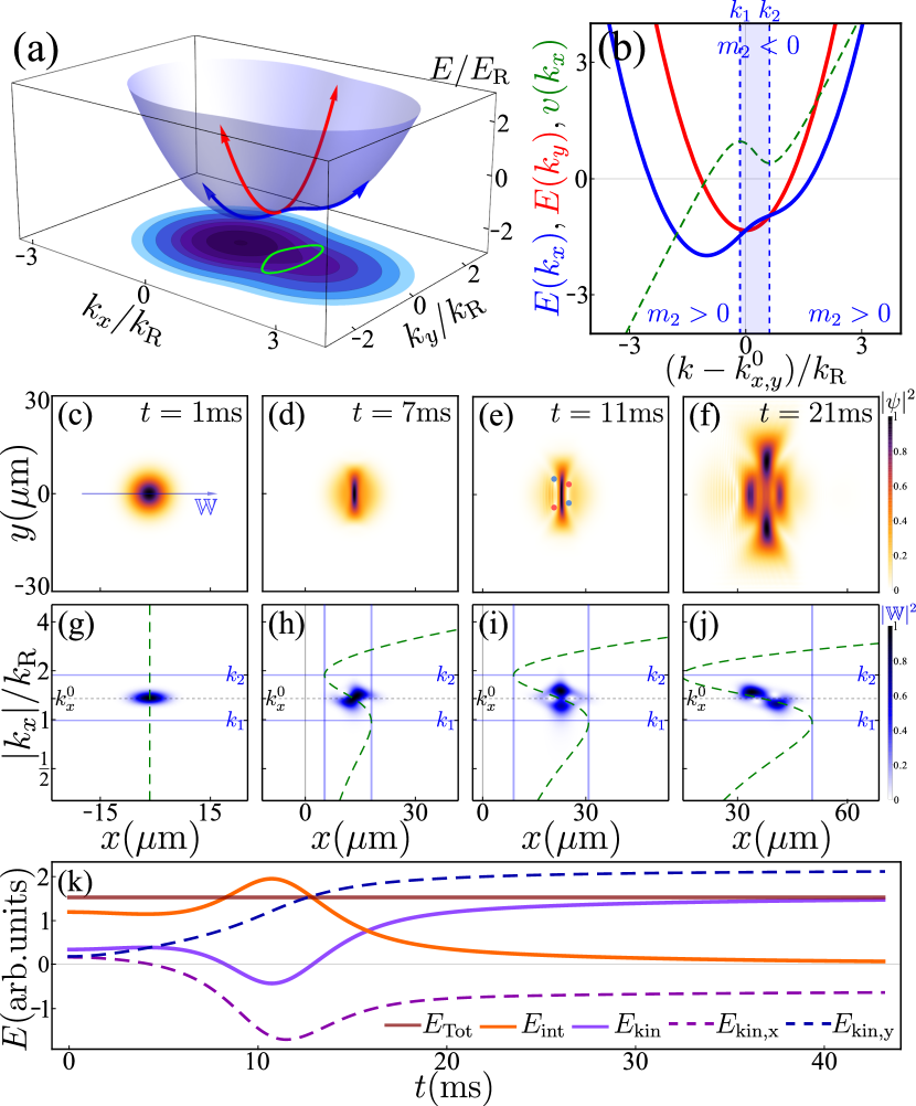
Figure 3: X-wave dynamics in a SOCBEC. (a) 2D-SOCBEC dispersion. The green line on the bottom projection encloses the inflection points region. (b) Effective dispersion in two transverse directions from the point $(k_{x}=1.35k_{\mathrm{R}},k_{y}=0)$, with $v_{x}(k)$. (c–f) Evolution of the atomic density $|\psi|^{2}$ at selected times. Light-blue (red) dots indicate a $\pm 2\pi$ phase winding. We note that the vortices present in frame (e) have moved outside of the boundary of frame (f) (g–j) Corresponding wavelet energy density $|\mathbb{W}|^{2}$ computed along the $x$ direction. The packet is imparted with a momentum $k_{x}^{0}$, between the inflection points $k_{1}$ and $k_{2}$. The green dashed curve shows the displacement of the $k_{x}$-components $d(k_{x})=v(k_{x})t$. The vertical blue lines correspond to displacements $d(k_{1})$ and $d(k_{2})$ delimiting the interference area. (k) Evolution of the different energies: total (brown), interaction (orange), kinetic (purple) with its two components along $x$ (dashed-dark purple) and y (dashed-dark blue). Supplemental Movie 3 provides an animation of the nonlinear X-wave formation for this system foo (b).

IV Spin-orbit coupled Bose-Einstein condensates

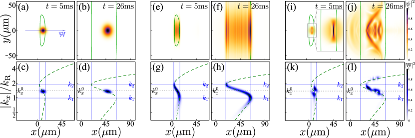
Figure 4: Wave packet propagation in 2D-SOCBEC. The top row shows the atomic density $|\psi(x,y)|^{2}$ at a given time of its evolution and the bottom row shows the corresponding wavelet energy density $|\mathbb{W}(x,k)|^{2}$, with a WT performed at $k_{y}=0$. The green line delimits the self-interference area. (a–d) Evolution from an initial Gaussian wave packet of width $\sigma_{\bm{r}}=$3.5\text{\,}\mathrm{\SIUnitSymbolMicro m}$$ in the linear regime ($g_{\mathrm{2D}}=0$). (e–h) Self-interfering regime, obtained from an initial Gaussian wave packet of width $\sigma_{\bm{r}}=$0.35\text{\,}\mathrm{\SIUnitSymbolMicro m}$$ in the linear regime ($g_{\mathrm{2D}}=0$). (i–l) The more strongly interacting regime compared to Fig. 3 with $g_{2D}N=14\times 10^{-4}E_{\mathrm{R}}$, from an initial Gaussian wave packet of width $\sigma_{\bm{r}}=$3.5\text{\,}\mathrm{\SIUnitSymbolMicro m}$$.

We finally consider a third condensed-matter system in which SIPs have been recently encountered in a one-dimensional setting — a 1D-spin-orbit coupled Bose-Einstein condensate (SOCBEC) Khamehchi et al. (2017); Colas et al. (2018). When extended to two dimensions, this system also possesses the key elements to generate nonlinear X-waves.

A non-interacting 2D-SOCBEC can be described by the following Hamiltonian Stanescu et al. (2008); Lin et al. (2011):

$$H_{\mathrm{SOC}}=\begin{pmatrix}\frac{\hbar(k_{x}^{2}+k_{y}^{2})}{2m}+\gamma k_{x}+\frac{\delta}{2}&\frac{\Omega}{2}\\ \frac{\Omega}{2}&\frac{\hbar(k_{x}^{2}+k_{y}^{2})}{2m}-\gamma k_{x}-\frac{\delta}{2}\end{pmatrix}\,,$$ (10)

which acts on the spinor field $\bm{\psi}=(\psi_{\uparrow},\psi_{\downarrow})^{T}$. Two hyperfine pseudo-spin states up $|{\uparrow}\rangle=|{F=1,m_{F}=0}\rangle$ and down $|{\downarrow}\rangle=|{F=1,m_{F}=-1}\rangle$ are coupled with the Raman coupling strength $\Omega$ and detuned by $\delta/2$. We also introduce $\gamma=\hbar k_{\mathrm{R}}/m$. The energy and momentum units are set by $E_{\mathrm{R}}=(\hbar k_{\mathrm{R}})^{2}/2m$, $E_{\mathrm{R}}$ and $k_{\mathrm{R}}$ being the recoil energy and the Raman wavevector, respectively.

Once diagonalised, the individual dispersion relations of the two spin states are mixed, leading to the upper ($+$) and lower ($-$) energy bands:

$$E_{\pm}(\bm{k})=\frac{\hbar(k_{x}^{2}+k_{y}^{2})}{2m}\pm\sqrt{\left(\gamma k_{x}+\frac{\delta}{2}\right)^{2}+\left(\frac{\Omega}{2}\right)^{2}}\,.$$ (11)

The lower band $E_{-}(\bm{k})$ is plotted in Fig. 3(a). Unlike the polariton dispersion, see Fig 2(a), the 2D-SOCBEC dispersion is not circularly symmetric and inflection points are only present in a finite region of momentum space foo (d). This region can be determined analytically. To do so, we make a change of coordinates ${k_{x}=k\cos(\theta),\,k_{y}=k\sin(\theta)}$ in Eq. (11) to obtain the dispersion relation $E(k,\theta)$ in polar coordinates. We can then find the inflection points of the dispersion for each specific angle $\theta$ by solving $\partial_{k}^{2}E(k,\theta)=0$. This yields the following expression:

$$k_{1,2}(\theta)=\frac{\delta}{4k_{\mathrm{R}}}\pm\frac{\sec\theta}{4k_{\mathrm{R}}}\sqrt{(2k_{\mathrm{R}}\Omega\cos\theta)^{\frac{4}{3}}-\Omega^{2}}\,.$$ (12)

These two solutions $k_{1,2}(\theta)$ are plotted as a light-green line in Fig. 3(a) and form the delimiting region of momentum space in which one can find a locally hyperbolic dispersion. From Eq. (11), one can also define the critical angle $\theta_{c}$ from which the dispersion is no longer hyperbolic:

$$\theta_{c}=\tan^{-1}\left[\frac{\sqrt{\Omega}}{k_{\mathrm{R}}}\bigg{/}\sqrt{4-\frac{\Omega}{k_{\mathrm{R}}^{2}}}\right]\,.$$ (13)

Corresponding to this hyperbolic region in momentum space, one can then define a corresponding velocity range in real space. For each point $(k_{x,i},k_{y,i})$ of the hyperbolic region limit—see the green curve in Fig. 3(a)—we can derive a corresponding velocity $(v_{x,i},v_{y,i})$ given by:

$$v_{x,i}=\partial_{k_{y}}E(k_{x,i},k_{y})\Bigr{\rvert}_{k_{y}=k_{y,i}}\,,$$ (14a)

$$v_{y,i}=\partial_{k_{x}}E(k_{x},k_{y,i})\Bigr{\rvert}_{k_{x}=k_{x,i}}\,.$$ (14b)

Finally from $(v_{x,i},v_{y,i})$, we can then obtain a set of coordinates defining a propagating distance $(d_{x,i},d_{y,i})=(v_{x,i}t,v_{y,i}t)$. This set $(d_{x,i},d_{y,i})$ defines a closed surface in real space, that increases with time. This area delimits the region of space into which self-interference can occur. This is the 2D equivalent of the “diffusion cone” previously derived in 1D Colas and Laussy (2016). X-waves can thus be generated by exciting $E_{-}(\bm{k})$ in this specific region, between two inflection points $k_{1}$ and $k_{2}$, where the effective dispersion appears locally hyperbolic.

The condensate dynamics can be obtained from a single-band 2D-Gross-Pitaevskii equation Khamehchi et al. (2017):

$$i\partial_{t}\psi(\bm{r})=\mathscr{F}^{-1}_{\bm{r}}[E_{-}(\bm{k})\psi(\bm{k})]+g_{\mathrm{2D}}|\psi(\bm{r})|^{2}\psi(\bm{r})\,,$$ (15)

where $E_{-}(\bm{k})$ is the lower band defined in Eq. (11). $\mathscr{F}^{-1}_{\bm{r}}$ indicates the 2D inverse Fourier transform, and $g_{\mathrm{2D}}$ the effective 2D interaction strength.

The experiment of Khamehchi et al. explored effectively one-dimensional dynamics, where the inital SOCBEC was released from its initial cigar-shaped harmonic trap into a waveguide Khamehchi et al. (2017). The SOCBEC interaction energy was transformed into kinetic energy, leading to a spread in momentum space across the inflection point of the dispersion, and the development of a SIP Khamehchi et al. (2017); Colas et al. (2018). Here we explore a similar scenario where a SOCBEC is released from a circularly symmetric harmonic trap into a two-dimensional waveguide, leading to the formation of a nonlinear X-wave.

As in the polariton case, only a weak nonlinearity is needed to trigger the X-wave formation in a SOCBEC. We choose $g_{2D}N=7\times 10^{-4}E_{\mathrm{R}}$, and an initial condensate size of $\sigma_{r}=$3.5\text{\,}\mathrm{\SIUnitSymbolMicro m}$$, assumed to be Gaussian in this regime foo (e); Pethick and Smith (2001). We impart an initial momentum to the wave packet of $(k_{x}^{0},k_{y}^{0})=(1.35,0)\times k_{\mathrm{R}}$ which is within the inflection point region of the dispersion, as shown in Fig. 3(a,b). In Fig. 3(c–f) we present selected time frames of the density evolution obtained from Eq. (15), along with the corresponding 1D-WT performed in the direction of propagation at $y=0$, Fig. (g–j). Once again, one can observe the mechanism leading to the X-wave formation, that is, the splitting of the wave packet into two sub-packets of different momenta in a configuration where the faster packet is in a position to overlap with the slower one and thus interfere with it. We note again the formation of vortex-antivortex pairs in Fig. 3(e), which have moved outside the boundary of Fig. 3(f).

We can perform a similar analysis for the energy of the system that we did for the ideal hyperbolic case. The evolution of the different energy components is presented in Fig. 3(k) and shows qualitatively the same features as the hyperbolic case previously shown in Fig. 1(k). One can, however, see that at $t=0$, the kinetic energy is not zero, since the 2D-SOCBEC dispersion does not possess the same $x$-$y$ symmetry.

For the parameters we have considered the nonlinearity is strong enough to form an X-wave, but remains weak enough to restrict the packet’s spread between the two inflection points $k_{1}$ and $k_{2}$. Increasing the effective interaction strength would increase the packet’s spread in momentum and lead to the formation of more complex wave structures in real space.

Without interactions ($g_{2D}=0$) the internal reshaping of the wave packet does not occur, and the condensate dynamics are simply those of a slowly diffusing wave packet as shown in Fig. 4(a–d). However, in this case the SIP regime can still be reached by setting a tight Gaussian as initial condition Colas and Laussy (2016). Such dynamics are shown in Fig. 4(e–h). The real space density $|\psi(x,y)|^{2}$ displays self-interference fringes fully bounded in the delimiting area $d(x_{i},y_{i})$ previously derived (green line). In the $x$-$k$ space representation, the wavelet energy density closely follows the displacement associated with each wave vector $d(k_{x},t)$. In the absence of interactions, the spread in momentum space is entirely defined from the initial condition through the wave packet’s width $\sigma_{\mathrm{r}}$.

Reaching the SIP regime requires a sufficiently broad wave packet in momentum space that straddles the inflection points. If the initial wave packet does not have this structure, it can be achieved by a transformation of interaction energy to kinetic energy Colas et al. (2018). To demonstrate this, we again take the configuration used to generate the X-wave as in Fig. 3, but with an interaction strength twice as large, $g_{2D}N=14\times 10^{-4}E_{\mathrm{R}}$, shown in Fig. 4(i–l). At early times an X-wave still forms thanks to the spread in momentum caused by the nonlinearity, as shown in Fig. 4(i). The corresponding wavelet transform shows the wave packet reshaping and the typical feature of an X-wave self-interference, Fig. 4(k). However, at longer times the X-wave shape in the density is no longer present and the density exhibits a considerably more complex structure. The wavelet analysis performed at this particular time of the evolution shows that the packet’s spread is now large enough to populate the dispersion above the second inflection point, which is typical of the SIP regime. This shows that X-waves generated in nonlinear systems only exist and propagate for a finite time, and that more complicated effects can follow in their wake.

The internal reshaping of the wave packet due to a nonlinearity leading to the X-wave formation is in many ways similar to the linear self-interfering effect previously described for 1D systems Colas and Laussy (2016); Colas et al. (2018). However the two mechanisms should not be confused, even if they can both occur during the same experiment, as shown in Fig. 4(i–l). The X-wave formation mechanism exploits the spread in momentum space provided by the nonlinear interaction to generate two distinct sub-packets, far from the inflections points (if any) in the negative effective mass region, overlapping and interfering in real space. On the other hand, the linear self-interference mechanism occurs due to the change of sign of the $k$-dependent group velocity at the inflection points to create an effective superposition across a broad and continuous range of momenta.

V Conclusions

In this paper we have shown that nonlinear X-waves, including those recently observed in excition-polariton systems, arise from an interference mechanism triggered by the nonlinear interaction. The interaction increases the packet’s spread in momentum space, leading to the formation of two effective sub-packets travelling at a different velocities, hence overlapping in space and interfering. The complex wave packet dynamics can be revealed and understood by utilising the wavelet transform. The key ingredient in the X-wave formation is the presence of a locally hyperbolic dispersion relation, and we have shown that similar X-waves can be obtained in other physical systems with this feature. For example, X-waves can be formed in SOCBECs in the weakly interacting regime without the need for an optical lattice potential. Overall, our analysis of the X-wave formation dynamics utilising the wavelet transform provides physically insight into otherwise puzzling wave packet dynamics, and has identified the central role of self-interference. This emphasizes the importance of the self-interfering packet effect for nonstandard dispersion relations either with or without the influence of nonlinearities.

The Supplemental Material for this manuscript includes movies of the full dynamics for the three different systems we have considered in each of Figs. 1, 2, 3 which shed further light on the nonlinear X-wave dynamics foo (b).